Off-policy Policy Evaluation For Sequential Decisions
Under Unobserved Confounding

Abstract

When observed decisions depend only on observed features, off-policy policy evaluation (OPE) methods for sequential decision making problems can estimate the performance of evaluation policies before deploying them. This assumption is frequently violated due to unobserved confounders, unrecorded variables that impact both the decisions and their outcomes. We assess robustness of OPE methods under unobserved confounding by developing worst-case bounds on the performance of an evaluation policy. When unobserved confounders can affect every decision in an episode, we demonstrate that even small amounts of per-decision confounding can heavily bias OPE methods. Fortunately, in a number of important settings found in healthcare, policy-making, operations, and technology, unobserved confounders may primarily affect only one of the many decisions made. Under this less pessimistic model of one-decision confounding, we propose an efficient loss-minimization-based procedure for computing worst-case bounds, and prove its statistical consistency. On two simulated healthcare examples—management of sepsis patients and developmental interventions for autistic children—where this is a reasonable model of confounding, we demonstrate that our method invalidates non-robust results and provides meaningful certificates of robustness, allowing reliable selection of policies even under unobserved confounding.

1 Introduction

New technology and regulatory shifts allow the collection of an unprecedented amount of data on past decisions and their associated outcomes, ranging from product recommendation systems to medical treatment decisions. This presents unique opportunities for using off-policy observational data to inform better decision-making. When online experimentation is expensive or risky, it is crucial to leverage prior data to evaluate the performance of a sequential decision policy (which we call the evaluation policy) before deploying it. The dynamic treatment regime literature (Robins, 1986, 1997; Murphy, 2003) addressed many early questions around using observational data for sequential decision making, and developed a rich set of methods adapted for epidemiological questions. The reinforcement learning (RL) community is increasingly interested in developing theory and methods for the related problem of batch RL across a broad set of applications, because of new models and data availability (see e.g. Thomas et al. (2019); Liu et al. (2018b); Le et al. (2019); Thomas et al. (2015); Komorowski et al. (2018b); Hanna et al. (2017); Gottesman et al. (2019b, c)). We focus on performing off-policy policy evaluation (OPE) in the common scenario where decisions are made in episodes by an unknown behavior policy, each involving a sequence of decisions.

A central challenge in OPE is that the estimand is inherently a counterfactual quantity: what would the resulting outcomes be if an alternate policy had been used (the counterfactual) instead of the behavior policy that generated the observed data (the factual). As a result, OPE requires causal reasoning about whether observed high/low rewards were caused by observed decisions, as opposed to a common causal variable that simultaneously affects both the observed decisions and the states or rewards (Hernán and Robins, 2020; Pearl, 2009). In order to make counterfactual evaluations possible, a standard assumption—albeit often overlooked and unstated—is to require that the behavior policy does not depend on any unobserved/latent variables that also affect the future states or rewards (no unobserved confounding). We refer to this assumption as sequential ignorability, following the line of works on dynamic treatment regimes (Robins, 1986, 1997; Murphy et al., 2001; Murphy, 2003).

Sequential ignorability, however, is almost always violated in observational problems where the behavior policy is unknown. In healthcare, business operations, and some automated systems in tech, decisions depend on unlogged features correlated with future outcomes. Clinicians use visual observations or discussions with patients to inform treatment decisions, but such information is typically not quantified and coded in electronic medical records; they also rely on heuristics that are fundamentally difficult to quantify, tending to over-extrapolate on past experience and slow to correct mistakes (McDonald, 1996). In judicial decisions, psychological factors affect bail and parole decisions (Dhami, 2003; Danziger et al., 2011). In business contexts, simple heuristics are prevalent; concrete examples include venture capital investments (Åstebro and Elhedhli, 2006), and customer targeting (Wübben and Wangenheim, 2008). Even automated policies in tech firms depend on unlogged features (Agarwal et al., 2016), and complex software and data infrastructures often introduce confounding.

In this paper, we study a framework for quantifying the impact of unobserved confounders on OPE estimates, developing worst-case bounds on the performance of an evaluation policy. Since OPE is generally impossible under arbitrary unobserved confounding, we begin by positing a model that explicitly limits their influence on decisions. Our proposed model is a natural extension of an influential confounding model for a single binary decision (Rosenbaum, 2002) to the multi-action sequential decision making setting. When unobserved confounders can affect all decisions, even small amounts of confounding can have an exponential (in the number of decisions) impact on the bias of OPE as we illustrate in Section 4. In this sense, the validity of OPE can almost always be questioned under presence of unobserved confounding that affect all decisions.

Fortunately, in a number of important applications, unobserved confounders may only affect a single decision. Frequently, this happens when a high-level expert decision-makers make an initial decision potentially using unrecorded information, after which a standard set of protocols are followed based on well-recorded observations. Under our less pessimistic model of single-decision confounding, we develop bounds on the expected cumulative rewards under the evaluation policy (Section 5). We use functional convex duality to derive a dual relaxation, and show that it can be computed by solving a loss minimization problem. Our procedure allows analyzing sensitivity of OPE methods to confounding in realistic scenarios involving continuous state and rewards, over a potentially large horizon. We prove that an empirical approximation of our procedure is consistent, allowing estimation from observed past decisions. Our loss minimization approach builds on the single decision work by Yadlowsky et al. (2018), and extends it to sequential decision-making scenarios.

On examples of dynamic treatment regimes for autism and sepsis management, we illustrate how our single-decision confounding model allows informative bounds over meaningful amounts of confounding. Our approach provides certificates of robustness by identifying the level of unobserved confounding at which the bias in OPE estimates can raise concerns about the validity of selecting the best policy among a set of candidates. As we illustrate, developing tools for a meaningful sensitivity analysis is nontrivial: a naive bound yields prohibitively conservative estimates that almost lose robustness certificates for even neglible amounts of confounding, whereas our loss-minimization-based bounds on policy values is informative.

1.1 Motivating example: managing sepsis patients

Sepsis in ICU patients accounts for 1/3 of deaths in hospitals (Howell and Davis, 2017). Sepsis treatment decisions are made by a clinical care team, including nurses, residents, and ICU attending physicians and specialists (Rhodes et al., 2017). Difficulties of care often lead to making decisions based off of imperfect information, leading to substantial room for improvement. AI-based approaches provide an opportunity for optimal automated management of medications, freeing the care team to allocate more resources to critical cases. Automated approaches can manage important medications for sepsis, including antibiotics and vasopressors, and decide to notify the care team about when a patient should be placed on a mechanical ventilator. Motivated by these opportunities, and the availability of ICU data from MIMIC-III (Johnson et al., 2016), several AI-based approaches for sepsis management system have been proposed (Futoma et al., 2018; Komorowski et al., 2018a; Raghu et al., 2017).

Due to safety concerns, new treatment policies need to be evaluated offline before thorough online clinical validation. Confounding, however, is a serious issue in data generated from an ICU. Patients in emergency departments often do not have an existing record in the hospital’s electronic health system, leaving a substantial amount of patient-specific information unobserved in subsequent offline analysis. As a prominent example, comorbidities that significantly complicate the cases of sepsis (Brent, 2017) are often unrecorded. Private communication with an emergency department physician revealed that initial treatment of antibiotics at admission to the hospital are often confounded by unrecorded factors that affect the eventual outcome (death or discharge from the ICU). For example, comorbidities such as undiagnosed heart failure can delay diagnosis of sepsis, leading to slower implementation of antibiotic treatments. More generally, there is considerable discussion in the medical literature on the importance of quickly beginning antibiotic treatment, with frequently noted concerns about confounding, as these discussions are largely based on off-policy observational data collected from ICUs (Seymour et al., 2017; Sterling et al., 2015). Given the recent interest in balancing early treatment with risks of over-prescription, treatment regimes for antibiotics are of particular interest.

We consider a scenario where one wishes to evaluate between two automated policies that differ only in initially avoiding, or prescribing antibiotics, and otherwise acts optimally. The latter is often considered a better treatment for sepsis, as it is caused by an infection. In this example, unobserved factors most critically effect the first decision on prescribing antibiotics upon arrival; since the care team is highly trained for treating sepsis, we assume they follow standard protocols based on observed vitals signs and lab measurements in subsequent time steps. In what follows, we assess the impact of confounding factors discussed above on OPE of automated policies, and provide certificates of robustness that guarantee gains over existing policies.

2 Related Work

The majority of OPE methods for batch reinforcement learning rely on sequential ignorability (though often unstated). There is an extensive body of work for off-policy policy evaluation and optimization under this assumption, including doubly robust methods (Jiang and Li, 2015; Thomas and Brunskill, 2016) and recent work that provides semiparametric efficiency bounds (Kallus and Uehara, 2019); often the behavior policy (conditional distribution of decisions given states) is assumed to be known. Notably, Liu et al. (2018b) highlights how estimation error in the behavioral policy can bias value estimates, and Nie et al. (2019); Hanna et al. (2019) provides OPE estimators based on an estimator of the behavior policy. When sequential ignorability doesn’t hold, the expected cumulative rewards under an evaluation policy cannot be identified from observable data. All of the above estimators are biased in the presence of unobserved confounding, since neither the outcome model nor the importance sampling weights can correct for the effect of the unobserved confounder.

The do-calculus and its sequential backdoor criterion on the associated directed acyclic graph (Pearl, 2009) also gives identification results for OPE. Like sequential ignorability, this preclude the existence of unobserved confounding variables. Therefore, methods that assume the sequential backdoor criterion will be biased in their presence.

We study the effects of unobserved confounding on OPE in sequential decision making problems, deriving bounds on the performance of the evaluation policy when sequential ignorability is relaxed. For problems where only one decision is made, a variety of methods developed in the econometrics, statistics, and epidemiology literature estimate bounds on treatment effects and expected rewards. Manski (1990) developed bounds that only assume bounded rewards, though they are too conservative to identify whether one action is superior to another. Then, Manski (1990) and other works posit models that bound the effect of unobserved confounding on the outcome (Robins et al., 2000; Brumback et al., 2004), or—like ours—on the actions taken by the behavior policy (Cornfield et al., 1959; Rosenbaum and Rubin, 1983; Imbens, 2003). Recent work studied approaches that can apply to heterogeneous treatment effects (Yadlowsky et al., 2018; Kallus et al., 2018), policy evaluation (Jung et al., 2018), and policy optimization (Kallus and Zhou, 2018).

In sequential decision making settings, Zhang and Bareinboim (2019) derived partial identification bounds on policy performance with limited restrictions on the influence of the unobserved confounder on observed decisions, much like the single decision work of Manski (1990), which they use to guide online RL algorithms. Unfortunately, these bounds are quite conservative for use only in OPE. Robins et al. (2000); Robins (2004); Brumback et al. (2004) instead posit a model for how the confounding bias in each time step affects the outcome of interest and derive bounds under this model: their work is motivated by potential confounding in the effects of dynamic treatment regimes for HIV therapy on CD4 counts in HIV-positive men. Our work is complementary to these in that we instead assume a model for how the unobserved confounder affects the actions taken by the behavior policy.

3 Formulation

Notation conventions vary substantially in the diverse set of communities interested in learning from (sequential) observational data. In this paper, we use the potential outcomes notation to make explicit which sequence of actions we wish to evaluate versus which sequence of actions were actually observed. In this approach, we posit all potential states and rewards exist for each possible sequence of actions, but we only observe the one corresponding to the actions taken (also known as partial, or bandit feedback), making the other potential states and rewards counterfactual. Literature in batch off policy reinforcement learning almost always assumes sequential ignorability, in which case the distribution of potential states and rewards are independent of the action taken by the behavior policy, conditional on the observed history. This allows us to consistently estimate counterfactuals simply based on observed outcomes. However, since our aim is to consider the impact of hypothetized confounding, clarifying the difference between the potential and observed states and rewards is cumbersome, but important.

We focus on domains modeled by episodic stochastic decision processes with a discrete set of actions. Let $\mathcal{A}_{t}$ be a finite action set of actions available at time $t=1,..,T$. Denote a sequence of actions $a_{1}\in\mathcal{A}_{1},..,a_{T}\in\mathcal{A}_{T}$ by $a_{1:T}$ (and similarly $a_{t:t^{\prime}}$ for arbitrary indices $1\leq t\leq t^{\prime}\leq T$, with the convention $a_{1:0}=\varnothing$). For any sequence of actions $a_{1:T}$, let $S_{t}(a_{1:t-1})$ and $R_{t}(a_{1:t})$ be the state and reward at time $t$. A state can be a scalar or a vector of discrete- or continuous-valued features; in our experimental settings we consider continuous-valued states. $Y(a_{1:T}):=\sum_{t=1}^{T}\gamma^{t-1}R_{t}(a_{1:t})$ is the corresponding discounted sum of rewards. We denote by $W(a_{1:T})=(S_{1},..,S_{T}(a_{1:T-1}),R_{1}(a_{1}),..,R_{T}(a_{1:T}))$ all potential outcomes (over rewards and states) associated with the action sequence $a_{1:T}$. Any sum $\sum_{a_{1:t}}$ over action sequences is taken over all $a_{1:T}\in\mathcal{A}_{1}\times\cdots\times\mathcal{A}_{T}$.

In the off-policy setting, we observe sequences of actions $A_{1},..,A_{T}$ generated by an unknown behavior policy $\pi_{1},..,\pi_{T}$. Let $H_{t}$ denote the observed history until time $t$, so that $H_{1}:=S_{1}$, and for $t=2,..,T$, $H_{t}:=(S_{1},A_{1},S_{2}(A_{1}),A_{2},..,S_{t}(A_{1:t-1}))$. As a notational shorthand, for any fixed sequence of actions $a_{1:T}$, denote an instantiation of the observed history following the action sequence by $H_{t}(a_{1:t-1})$, so that $H_{1}(a_{1:0}):=H_{1}=S_{1}$, and for $t=2,..,T$, $H_{t}(a_{1:t-1})=(S_{1},A_{1}=a_{1},S_{2}(a_{1}),..,A_{t-1}=a_{t-1},S_{t}(a_{1:t-1}))$. Let $\mathcal{H}_{t}$ be the set over which this history takes values.

When there is no unobserved confounding, $A_{t}\sim\pi_{t}(\cdot\mid H_{t})$ since actions are generated conditional on the observed history $H_{t}$. When there is unobserved confounding $U_{t}$, the behavioral policy draws actions $A_{t}\sim\pi_{t}(\cdot\mid H_{t},U_{t})$, and we denote by $\pi_{t}(\cdot\mid H_{t})$ the conditional distribution of $A_{t}$ given only the observed history $H_{t}$, meaning we marginalize out the unobserved confounder $U_{t}$. For simplicity, we assume that previously observed rewards are included in the states, so for $s<t$, $R_{s}(A_{1:s})$ is known given $H_{t}$ the history. We define $Y_{t}(a_{t}):=Y(A_{1:t-1},a_{t},A_{t+1:T})$ as a shorthand: semantically this means the sum of rewards which matches a trajectory of executed actions on all but one action, where on time step $t$ action $a_{t}$ is taken. Note that since $a_{t}$ may not be identical to the taken action $A_{t}$, the resulting expression for $Y$ represents a potential outcome.

Our goal is to bound the performance of an evaluation policy $\bar{\pi}_{1},..,\bar{\pi}_{T}$ in a confounded sequential off-policy environment. Let $\bar{A}_{t}\sim\bar{\pi}_{t}(\cdot\mid\bar{H}_{t})$ be the actions generated by the evaluation policy at time $t$, where we use $\bar{H}_{t}:=(S_{1},\bar{A}_{1},S_{2}(\bar{A}_{1}),\bar{A}_{2},..,S_{t}(\bar{A}_{1:t-1}))$ and $\bar{H}_{t}(a_{1:t-1}):=(S_{1},\bar{A}_{1}=a_{1},S_{2}(a_{1}),\bar{A}_{2}=a_{2},..,S_{t}(a_{1:t-1}))$ to denote the history under the evaluation policy, analogously to the shorthands $H_{t},H_{t}(a_{1:t-1})$; $\bar{H}_{t}$ are mathematical constructs, as they are never observed in the behavioral data. We are interested in statistical estimation of the expected cumulative reward $\mathbb{E}[Y(\bar{A}_{1:T})]$ under the evaluation policy, which we call the performance of the evaluation policy (aka $V^{\bar{\pi}}$ in batch RL). Throughout, we assume $\pi_{t}(a_{t}\mid H_{t})>0$ whenever $\bar{\pi}_{t}(a_{t}\mid\bar{H}_{t})>0$, for all $t$ and $a_{t}$, and almost every $H_{t}$,: in other words, overlap holds with respect to the conditional distributions over actions given only the histories between the behavior policy and the evaluation policy.

We now state the sequential ignorability assumption in terms of the relationship between actions and potential outcomes (see e.g (Robins, 1986, 2004; Murphy, 2003)).

Definition 1 (Sequential Ignorability).

We say that a policy satisfies sequential ignorability if for all $t=1,..,T$, conditional on the history generated by the policy, the action generated by the policy is independent of the potential outcomes $R_{t}(a_{1:t}),S_{t+1}(a_{1:t}),R_{t+1}(a_{1:t+1}),S_{t+2}(a_{1:t+1}),..,$ $S_{T}(a_{1:T-1}),R_{T}(a_{1:T})$ for all $a_{1:T}\in\mathcal{A}_{1}\times\cdots\mathcal{A}_{T}$.

Sequential ignorability is a natural condition required for the evaluation policy to be well-defined: any additional randomization used by the evaluation policy $\bar{\pi}_{t}(\cdot\mid\bar{H}_{t})$ cannot depend on unobserved confounders. We assume that the evaluation policy always satisfies this assumption.

Assumption A.

The evaluation policy satisfies sequential ignorability (Definition 1).

Off-policy policy evaluation fundamentally requires counterfactual reasoning since we only observe the state evolution $S_{t}(A_{1:t-1})$ and rewards $R_{t}(A_{1:t})$ corresponding to the actions made by the behavioral policy. The canonical assumption in batch off-policy reinforcement learning is that sequential ignorability holds for the behavior policy. We now briefly review how this allows identification (and thus, accurate estimation) of $\mathbb{E}[Y(\bar{A}_{1:T})]$, the value of the evaluation policy.

Because we only observe potential outcomes $W(A_{1:t})$ evaluated at the actions $A_{1:t}$ taken by the behavior policy $\pi_{t}$, we need to express $\mathbb{E}[Y(\bar{A}_{1:T})]$ in terms of observable data generated by the behavioral policy $\pi_{t}$. Sequential ignorability of both the behavior policy and evaluation policy allows such counterfactual reasoning. The following identity is standard; we give its proof in Section B.1 for completeness. To ease notation, we write

$$\rho_{t}:=\frac{\bar{\pi}_{t}(A_{t}\mid\bar{H}_{t}(A_{1:t-1}))}{\pi_{t}(A_{t}\mid H_{t})}.$$ (1)

Lemma 1.

Assume sequential ignorability (Definition 1) holds for both the behavior and evaluation policy. Then, $\mathbb{E}[Y(\bar{A}_{1:T})]=\mathbb{E}[Y(A_{1:T})\prod_{t=1}^{T}\rho_{t}].$

The RHS is called the importance sampling formula.

4 Bounds under unobserved confounding

Despite the advantageous implications, it is often unrealistic to assume that the behavior policy $\pi_{t}$ satisfies sequential ignorability (Definition 1). We now relax the sequential ignorability of the behavior policy, and instead posit a model of bounded confounding for the behavior policy, then develop worst-case bounds on the evaluation policy performance $\mathbb{E}[Y(\bar{A}_{1:T})]$ under this model. In addition to the observed state $S_{t}(A_{1:t-1})$ available in the data, we assume that there is an unobserved confounder $U_{t}$ available only to the behavior policy at each time $t$. The behavior policy observes the history $H_{t}$ and the unobserved confounder $U_{t}$, and generates an action $A_{t}\sim\pi_{t}(\cdot\mid H_{t},U_{t})$. If $U_{t}$ contains information about unseen potential outcomes, then sequential ignorability (Definition 1) will fail to hold for the behavior policy.

Without loss of generality, let $U_{t}$ be such that the potential outcomes are independent of $A_{t}$ when controlling for $U_{t}$ alongside the observed states. Such an unobserved confounder always exists since we can define $U_{t}$ to be the tuple of all unseen potential outcomes.

Assumption B.

For all $t=1,..,T$, there exists a random vector $U_{t}$ such that conditional on the history $H_{t}$ generated by the behavior policy and $U_{t}$, $A_{t}\sim\pi_{t}(\cdot\mid H_{t},U_{t})$ is independent of the potential outcomes $R_{t}(a_{1:t}),S_{t+1}(a_{1:t}),R_{t+1}(a_{1:t+1}),S_{t+2}(a_{1:t+1}),..,$ $S_{T}(a_{1:T-1}),R_{T}(a_{1:T})$ for all $a_{1:T}\in\mathcal{A}_{1}\times\cdots\mathcal{A}_{T}$.

Identification of $\mathbb{E}[Y(\bar{A}_{1:T})]$ is impossible under arbitrary unobserved confounding. However, it is often plausible to posit that the unobserved confounder $U_{t}$ has a limited influence on the decisions of the behavior policy. When the influence of unobserved confounding on each action is limited, we may expect OPE estimates that (incorrectly) assume sequential ignorability may not be too biased.

Consider the following model of unobserved confounding for sequential decision making problems, which bounds confounder’s influence on the behavior policy’s decisions.

Assumption C.

For $t=1,..,T$, there is a $\Gamma_{t}\geq 1$ satisfying

$$\frac{\pi_{t}(a_{t}\mid H_{t},U_{t}=u_{t})}{\pi_{t}(a_{t}^{\prime}\mid H_{t},U_{t}=u_{t})}\frac{\pi_{t}(a_{t}^{\prime}\mid H_{t},U_{t}=u_{t}^{\prime})}{\pi_{t}(a_{t}\mid H_{t},U_{t}=u_{t}^{\prime})}\leq\Gamma_{t}$$ (2)

for any $a_{t},a_{t}^{\prime}\in\mathcal{A}_{t}$, almost surely over $H_{t}$, and $u_{t},u_{t}^{\prime}$, and sequential ignorability holds conditional on $H_{t}$ and $U_{t}$.

Our bounded unobserved confounding assumption (2) is a natural extension of a classical model of confounding proposed by Rosenbaum (2002) for a single decision ($T=1$) to sequential problems. When the action space is binary $\mathcal{A}_{t}=\{0,1\}$, the above bounded unobserved confounding assumption is equivalent (Rosenbaum, 2002) to the following logistic model $\log\frac{\mathbb{P}(A_{t}=1\mid H_{t},U_{t})}{\mathbb{P}(A_{t}=0\mid H_{t},U_{t})}=\kappa(H_{t})+(\log\Gamma_{t})\cdot b(U_{t})$ for some measurable function $\kappa(\cdot)$ and a bounded measurable function $b(\cdot)$ taking values in $[0,1]$.

In the sequential setting where $T>1$, OPE is almost always unreliable even under the aformentioned model. Effects of confounding can create exponentially large (in the horizon $T$) over-sampling of large (or small) rewards, introducing an extremely large, un-correctable bias. As an illustration, consider applying OPE in the following simplified setting, where there are no states. Let $U\sim\mbox{Unif}(\{0,1\})$ be a single unobserved confounder, and consider the sequence of behavioral actions $A_{1},\dots,A_{T}\in\{0,1\}$ each drawn conditionally on $U$, but independent of one another, with the conditional distribution $P(A_{t}=1\mid U=1)=\sqrt{\Gamma}/(1+\sqrt{\Gamma})$ and $P(A_{t}=1\mid U=0)=1/(1+\sqrt{\Gamma})$. Let the outcome be $Y(a_{1:T})=U$ for all possible action sequences $a_{1:T}$. Although the actions do not affect the outcome, in the observed data the likelihood of observing $((A_{t}=1)_{t=1}^{T},Y=1)$ is $\Gamma^{T/2}/(2(1+\sqrt{\Gamma})^{T})$, whereas the likelihood of observing $((A_{t}=1)_{t=1}^{T},Y=0)$ is $1/(2(1+\sqrt{\Gamma})^{T})$. Therefore, even in the limit of infinite observations, OPE will mistakenly estimate that always taking $\bar{A}_{t}=1$ leads to better rewards than always taking $\bar{A}_{t}=0$.

Even in this toy example example where states don’t exist and rewards don’t depend on actions, the effect of confounding is salient. The unobserved confounder can make certain observed data samples exponentially more likely than others, without the OPE algorithm being able to tell or correct for these differences. This has important implications for off-policy policy selection or optimization, where such systematic differences can lead to selection of a poorly performing policy.

5 Confounding in a single decision

In many important applications, it is realistic to assume there is only a single step of confounding at a known time step $t^{*}$. Under this assumption, we outline in this section how we obtain a computationally and statistically feasible procedure for computing a lower (or upper) bound on the value $\mathbb{E}[Y(\bar{A}_{1:T})]$ of an evaluation policy $\bar{\pi}$. After introducing precisely our model of confounding, we show in Proposition 1 how the evaluation policy value can be expressed using likelihood ratios over potential outcomes that can be used to relate the potential outcomes over observed (factual) actions with counterfactual actions not taken. These likelihood ratios over potential outcomes are unobserved, but a lower bound on the evaluation policy value can be computed by minimizing over all feasible likelihood ratios that satisfy our model of bounded confounding. Towards computational tractability, we derive a dual relaxation that can be represented as a loss minimization procedure.

We define the confounding model for when there is an unobserved confounding variable $U$ that only affects the behavior policy’s action at a single time period $t^{\star}\in[T]$. For example, in looking at the impact of confounders on antibiotics in sepsis management (Section 1.1), it is plausible to assume that while confounders may influence the first decision when the patient arrives, later treatment decisions are not impacted by unobserved confounders.

Assumption D.

For all $t\neq t^{\star}$, conditional on the history $H_{t}$ generated by the behavior policy, $A_{t}$ is independent of the potential outcomes $R_{t}(a_{1:t}),S_{t+1}(a_{1:t}),R_{t+1}(a_{1:t+1}),S_{t+2}(a_{1:t+1}),..,$ $S_{T}(a_{1:T-1}),R_{T}(a_{1:T})$ for all $a_{1:T}\in\mathcal{A}_{1}\times\cdots\mathcal{A}_{T}$. For $t=t^{\star}$, there exists a random variable $U$ such that the same conditional independence holds only when conditional on the history $H_{t}$ and $U$.

Similar to Assumption C, but now restricted to a single time step $t^{*}$, we assume the unobserved confounder has bounded influence on the behavior policy’s action $A_{t^{\star}}$.

Assumption E.

There is a $\Gamma\geq 1$ satisfying

$$\frac{\pi_{t^{\star}}(a_{t^{\star}}\mid H_{t^{\star}},U=u)}{\pi_{t^{\star}}(a_{t^{\star}}^{\prime}\mid H_{t^{\star}},U=u)}\frac{\pi_{t^{\star}}(a_{t^{\star}}^{\prime}\mid H_{t^{\star}},U=u^{\prime})}{\pi_{t^{\star}}(a_{t^{\star}}\mid H_{t^{\star}},U=u^{\prime})}\leq\Gamma$$ (3)

for any $a_{t^{\star}},a_{t^{\star}}^{\prime}\in\mathcal{A}_{t^{\star}}$, almost surely over $H_{t^{\star}}$, and $u,u^{\prime}$.

Selecting the amount of unobserved confounding $\Gamma$ is a modeling task, and the above confounding model’s simplicity and interpretability makes it advantageous for enabling modelers to choose a plausible value of $\Gamma$. As in any applied modeling problem, the amount of unobserved confounding $\Gamma$ should be chosen with expert knowledge (e.g. by consulting doctors that make behavioral decisions). In Section 6, we give various application contexts in which a realistic range of $\Gamma$ can be posited. One of the most interpretable ways to assess the level of robustness to confounding is via the design sensitivity of the analysis (Rosenbaum, 2010): the value of $\Gamma$ at which the bounds on the evaluation policy’s value crosses a landmark threshold (e.g. performance of behavior policy or some known safety threshold).

We first show that a simple naïve lower bound on the evaluation policy performance $\mathbb{E}[Y(\bar{A}_{1:T})]$ can be obtained by directly applying our bounded confounding model (3) to adjust the weights of an importance sampling estimator. Details are provided in Section C.1.

Lemma 2.

Let Assumptions A, D, E hold. Then, we have

$$\mathbb{E}[Y(\bar{A}_{1:T})]\geq\mathbb{E}\Bigg{[}Y(A_{1:T})\times\prod_{t=1}^{T}\rho_{t}$$ (4)

$$\qquad\times\left(\Gamma\mathbf{1}\left\{Y(A_{1:T})<0\right\}+\Gamma^{-1}\mathbf{1}\left\{Y(A_{1:T})>0\right\}\right)\Bigg{]}.$$

However, the naive bound (4) is often prohibitively conservative, as we concretely illustrate in Section 6.

Instead we derive a tighter bound on the evaluation policy performance $\mathbb{E}[Y(\bar{A}_{1:T})]$ based on a constrained convex optimization formulation over counterfactual distributions. Under Assumption E, the likelihood ratio between observed and unobserved distribution at $t^{\star}$ can at most vary by a factor of $\Gamma$. Recall that $W(a_{1:T})$ is the tuple of all potential outcomes associated with the actions $a_{1:T}$. The following observation is due to Yadlowsky et al. (2018, Lemma 2.1).

Lemma 3.

Under Assumptions D, E, for all $a_{t^{\star}}\neq a_{t^{\star}}^{\prime}$, the likelihood ratio over the tuple of potential outcomes $W:=\{W(a_{1:T})\}_{a_{1:T}}$ exists

$$\mathcal{L}(\cdot;H_{t^{\star}},a_{t^{\star}},a_{t^{\star}}^{\prime}):=\frac{dP_{W}(\cdot\mid H_{t^{\star}},A_{t^{\star}}=a_{t^{\star}}^{\prime})}{dP_{W}(\cdot\mid H_{t^{\star}},A_{t^{\star}}=a_{t^{\star}})},$$

and for $\mathbb{P}_{W}(\cdot\mid H_{t^{\star}},A_{t^{\star}}=a_{t^{\star}})$-a.s. all $w,w^{\prime}$

$$\mathcal{L}(w;H_{t^{\star}},a_{t^{\star}},a_{t^{\star}}^{\prime})\leq\Gamma\mathcal{L}(w^{\prime};H_{t^{\star}},a_{t^{\star}},a_{t^{\star}}^{\prime}).$$ (5)

We let $\mathcal{L}(\cdot;H_{t^{\star}},a_{t^{\star}},a_{t^{\star}})\equiv 1$. Using these (unknown) likelihood ratios, we can express the value of the evaluation policy, $\mathbb{E}[Y(\bar{A}_{1:T})]$.

Proposition 1.

Under Assumptions A, D, E,

$$\mathbb{E}[Y(\bar{A}_{1:T})]$$

$$=\mathbb{E}\Bigg{[}\prod_{t=1}^{t^{\star}-1}\rho_{t}\sum_{a_{t^{\star}},a_{t^{\star}}^{\prime}}\bar{\pi}_{t^{\star}}(a_{t^{\star}}\mid\bar{H}_{t^{\star}}(A_{1:t^{\star}-1}))\pi_{t^{\star}}(a_{t^{\star}}\mid H_{t^{\star}})$$

$$\times\mathbb{E}\Big{[}\mathcal{L}(W;H_{t^{\star}},a_{t^{\star}},a_{t^{\star}}^{\prime})Y(A_{1:T})\prod_{t=t^{\star}+1}^{T}\rho_{t}~{}\Big{|}~{}H_{t^{\star}},A_{t^{\star}}=a_{t^{\star}}\Big{]}\Bigg{]}.$$

The proof is given in Section B.2.

Proposition 1 implies a natural bound on the evaluation policy value $\mathbb{E}[Y(\bar{A}_{1:T})]$ under bounded unobserved confounding. Since the likelihood ratios $\mathcal{L}(\cdot;\cdot,a_{t^{\star}},a_{t^{\star}}^{\prime})$ are fundamentally unobservable due to their counterfactual nature, we take a worst-case approach over all likelihood ratios that satisfy condition (5), and derive a bound that only depend on observable distributions. Towards this goal, define

$$\mathfrak{L}:=\big{\{}L:\mathcal{W}\times\mathcal{H}_{t^{\star}}\to\mathbb{R}_{+}\mid L(w;H_{t^{\star}})\leq\Gamma L(w^{\prime};H_{t^{\star}})$$

$$\mbox{a.s. all}~{}w,w^{\prime},~{}\mbox{and}~{}\mathbb{E}[L(W;H_{t^{\star}})\mid H_{t^{\star}},A_{t^{\star}}=a_{t^{\star}}]=1\big{\}}.$$ (6)

Taking the infimum over the inner expectation in the expression derived in Proposition 1, and noting that it does not depend on $a_{t^{\star}}^{\prime}$, define

$$\eta^{\star}(H_{t^{\star}};a_{t^{\star}}):=$$

$$\inf_{L\in\mathfrak{L}}\mathbb{E}\left[L(W;H_{t^{\star}})Y(A_{1:T})\prod_{t=t^{\star}+1}^{T}\rho_{t}~{}\Big{|}~{}H_{t^{\star}},A_{t^{\star}}=a_{t^{\star}}\right].$$

Since the above optimization is over infinite-dimensional likelihoods, it is difficult to compute. We use functional convex duality to derive a dual relaxation that can be computed by solving a loss minimization problem over any well-specified model class. This allows us to compute a meaningful lower bound to $\mathbb{E}[Y(\bar{A}_{1:T})]$ even when rewards and states are continuous, by simply fitting a model using standard supervised learning methods. For $(s)_{+}=\max(s,0)$ and $(s)_{-}=-\min(s,0)$, define the weighted squared loss $\ell_{\Gamma}(z):=\frac{1}{2}(\Gamma(z)_{-}^{2}+(z)_{+}^{2})$.

Theorem 2.

Let Assumptions A, D, E hold. If $\mathbb{E}[Y(A_{1:T})^{2}\prod_{t=t^{\star}+1}^{T}\rho_{t}^{2}\mid A_{t^{\star}}=a_{t^{\star}},H_{t^{\star}}]<\infty$ a.s., then $\eta^{\star}(H_{t^{\star}};a_{t^{\star}})$ is lower bounded a.s. by the unique solution

$$\kappa^{\star}(H_{t^{\star}};a_{t^{\star}})=\mathop{\rm argmin}_{f(H_{t^{\star}})}~{}~{}\mathbb{E}\Bigg{[}\frac{\mathbf{1}\left\{A_{t^{\star}}=a_{t^{\star}}\right\}}{\pi_{t^{\star}}(a_{t^{\star}}\mid H_{t^{\star}})}$$

$$\qquad\qquad\times\ell_{\Gamma}\left(Y(A_{1:T})\prod_{t=t^{\star}+1}^{T}\rho_{t}-f(H_{t^{\star}})\right)\Bigg{]}.$$

See Section C.2 for the proof. From Theorem 2 and Proposition 1, our final lower bound on $\mathbb{E}[Y(\bar{A}_{1:T})]$ is given by

$$\mathbb{E}\Bigg{[}\prod_{t=1}^{t^{\star}-1}\rho_{t}\sum_{a_{t^{\star}}}\bar{\pi}_{t^{\star}}(a_{t^{\star}}\mid\bar{H}_{t^{\star}}(A_{1:t^{\star}-1}))$$

$$\qquad\times(1-\pi_{t^{\star}}(a_{t^{\star}}\mid H_{t^{\star}}))\kappa^{\star}(H_{t^{\star}};a_{t^{\star}})\Bigg{]}$$

$$+\mathbb{E}\left[\pi_{t^{\star}}(A_{t^{\star}}\mid H_{t^{\star}})Y(A_{1:T})\prod_{t=1}^{T}\rho_{t}\right].$$ (7)

Our approach yields a loss minimization problem for each possible action, where the dimension of this supervised learning problem is that of the observed history $H_{t^{*}}$ generated from the behavior policy. If confounding occurs early in the process ($t^{\star}\approx 1$), the space of possible histories is small and this learning problem becomes easier. This is the scenario for the domains we consider in our experiments.

In cases where there is low, yet sufficient, overlap, WIS can dramatically reduce variance, at the cost of increased bias, with respect to the usual IS estimator. While our approach uses the IS to adjust for the differences between the behavior and evaluation policy, adjusting the bound in (7) to use WIS, instead, is straightforward. Altering the importance reweighting inside the loss function for $\kappa^{\star}$ to be normalized, like WIS, warrants further investigation.

Yadlowsky et al. (2018) takes a similar approach to bound the effect of confounding on treatment effects when there is only one action taken. Our approach allows for comparing sequences of actions derived according to an evaluation policy, by adjusting for the way actions in all time steps depend on the current states and history, and effect future states and rewards. One notable challenge that only occurs in sequential problems is adjusting for actions that occur after the confounded decision at time $t^{\star}$; these actions depend on the confounded decision through the history generated. A natural approach is to individually bound the potential outcomes $\mathbb{E}[Y(\bar{A}_{1:t^{\star}-1},a_{t^{\star}:T})]$ for all $a_{t^{\star}:T}$, where each bound is given by a loss minimization problem. Under this approach—which is analogous to that of Yadlowsky et al. (2018) in the single time step—computing a lower bound to $\mathbb{E}[Y(\bar{A}_{1:T})]$ requires $\prod_{t=t^{\star}}^{T}|\mathcal{A}_{t}|$ loss minimization problems, making it statistically and computationally intractable when $t^{\star}$ is small (e.g. $t^{\star}=1$ in our sepsis example). Instead, we consider averaged outcomes $\mathbb{E}[Y(\bar{A}_{1:t^{\star}-1},a_{t^{\star}},\bar{A}_{t^{\star}+1:T})]$ in Theorem 2, which allows us to obtain a lower bound on $\mathbb{E}[Y(\bar{A}_{1:T})]$ by only solving $|\mathcal{A}_{t^{\star}}|$ loss minimization problems.

Consistency

We now show that an empirical approximation to our loss minimization problem yields a consistent estimate of $\kappa^{\star}(\cdot)$. We require the following standard overlap assumption, which states that actions cannot be too rare under the behavior policy, relative to the evaluation policy.

Assumption F.

There is $C\in(1,\infty)$ s.t. $\forall t$, $\rho_{t}\leq C$, a.s..

Since it is not feasible to optimize over the class of all functions $f(H_{t^{\star}})$, we consider a parameterization $f_{\theta}(H_{t^{\star}})$ where $\theta\in\mathbb{R}^{d}$. We provide provable guarantees in the simplified setting where $\theta\mapsto f_{\theta}$ is linear, so that the loss minimization problem is convex. That is, we assume that $f_{\theta}$ is represented by a finite linear combination of some arbitrary basis functions of $H_{t^{\star}}$. As long as the parameterization is well-specified so that $\kappa^{\star}(H_{t^{\star}};a_{t^{\star}})=f_{\theta^{\star}}(H_{t^{\star}})$ for some $\theta^{\star}\in\Theta$, an empirical plug-in solution converges to $\kappa^{\star}$ as the number of samples $n$ grows to infinity. We let $\Theta\subseteq\mathbb{R}^{d}$ be our model space; our theorem allows $\Theta=\mathbb{R}^{d}$.

In the below result, let $\widehat{\pi}_{t}(a_{t}\mid H_{t})$ be a consistent estimator of $\pi_{t}(a_{t}\mid H_{t})$ trained on a separate dataset $\mathcal{D}_{n}$ with the same underlying distribution; such estimators can be trained using sample splitting and standard supervised learning methods. Define the set $S_{\epsilon}$ of $\epsilon$-approximate optimizers of the empirical plug-in problem

$$\min_{f(H_{t^{\star}})}\widehat{\mathbb{E}}_{n}\left[\frac{\mathbf{1}\left\{A_{t^{\star}}=a_{t^{\star}}\right\}}{\widehat{\pi}_{t^{\star}}(a_{t^{\star}}\mid H_{t^{\star}})}\ell_{\Gamma}\left(Y(A_{1:T})\prod_{t=t^{\star}+1}^{T}\widehat{\rho}_{t}-f(H_{t^{\star}})\right)\right],$$

where $\widehat{\mathbb{E}}_{n}$ is the empirical distribution on the data statistically independent from $\mathcal{D}_{n}$, and

$$\widehat{\rho}_{t}:=\frac{\bar{\pi}(A_{t}\mid\bar{H}_{t}(A_{1:t-1}))}{\widehat{\pi}_{t}(A_{t}\mid H_{t}(A_{1:t-1}))}.$$

We assume we observe i.i.d. episodes, and that each episode (unit) does not affect one another, so the observed cumulative reward is the evaluation of the potential outcome at the observed action sequence, $Y(A_{1:T})$. We prove the below result in Section C.3.

Theorem 3.

Let Assumptions A, D,  E, F hold, and let $\theta\mapsto f_{\theta}$ be linear such that $f_{\theta^{\star}}(\cdot)=\kappa^{\star}(\cdot,a_{t^{\star}})$ for some unique $\theta^{\star}\in\mathbb{R}^{d}$. Let $\mathbb{E}|Y(A_{1:T})|^{4}<\infty$, and $\mathbb{E}[|f_{\theta}(H_{t^{\star}})|^{4}]<\infty$ for all $\theta\in\Theta$. If for all $t$, $\widehat{\pi_{t}}(\cdot|\cdot)\to\pi_{t}(\cdot|\cdot)$ pointwise a.s., $\widehat{\rho}_{t}\leq 2C$, and $(2C)^{-1}\leq\widehat{\pi}_{t^{\star}}(a_{t^{\star}}|H_{t^{\star}})\leq 1$ a.s., then $\liminf_{n\to\infty}\mbox{dist}(\theta^{\star},S_{\varepsilon_{n}})\stackrel{{\scriptstyle p}}{{\rightarrow}}0~{}\forall\varepsilon_{n}\downarrow 0$.

Hence, under the hypothesis of Theorem 3, a plug-in estimator of the lower bound (7) is consistent as $n\to\infty$.

6 Experiments

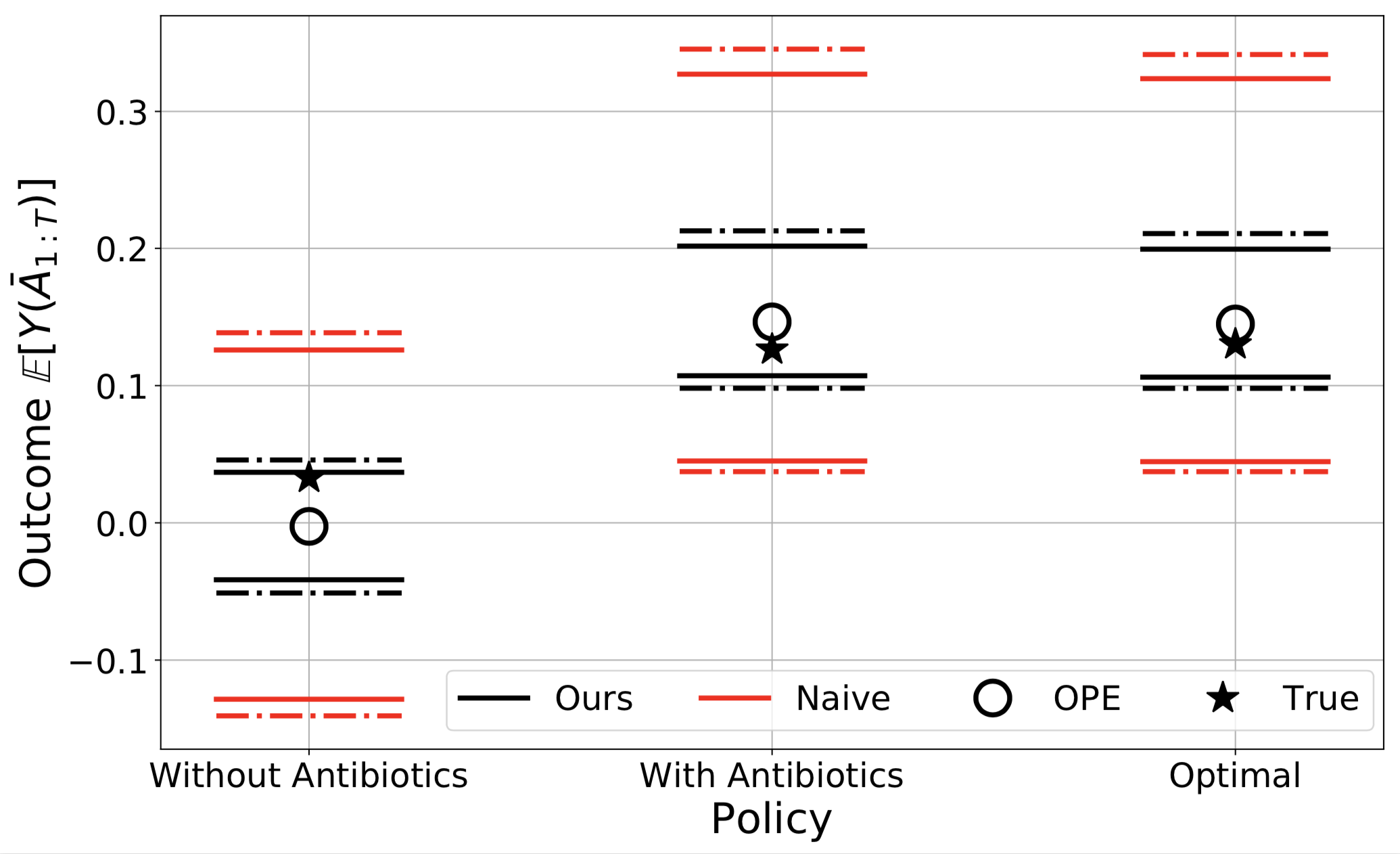
Figure 1: Sepsis simulation. Data generation process with the level of confounding $\Gamma^{\star}=2.0$. Each policies’ true value is shown with a start and a standard OPE estimate (ignoring confounding) is shown with an empty circle. Black lines show the estimated upper and lower bound on policy performance using our approach and red lines correspond to the naïve approach, both using $\Gamma=2.0$. Dashed lines represents $95\%$ quantile.

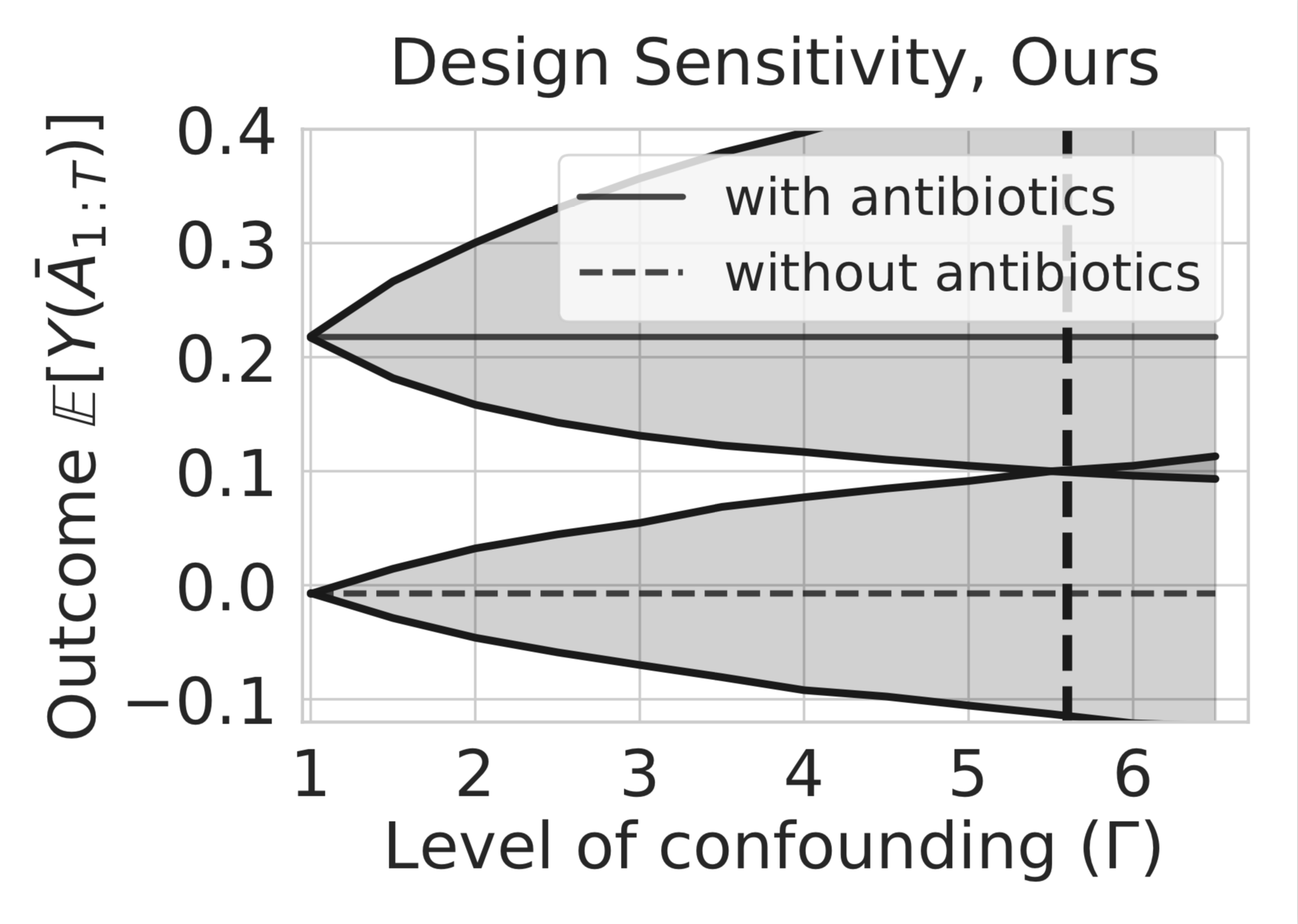
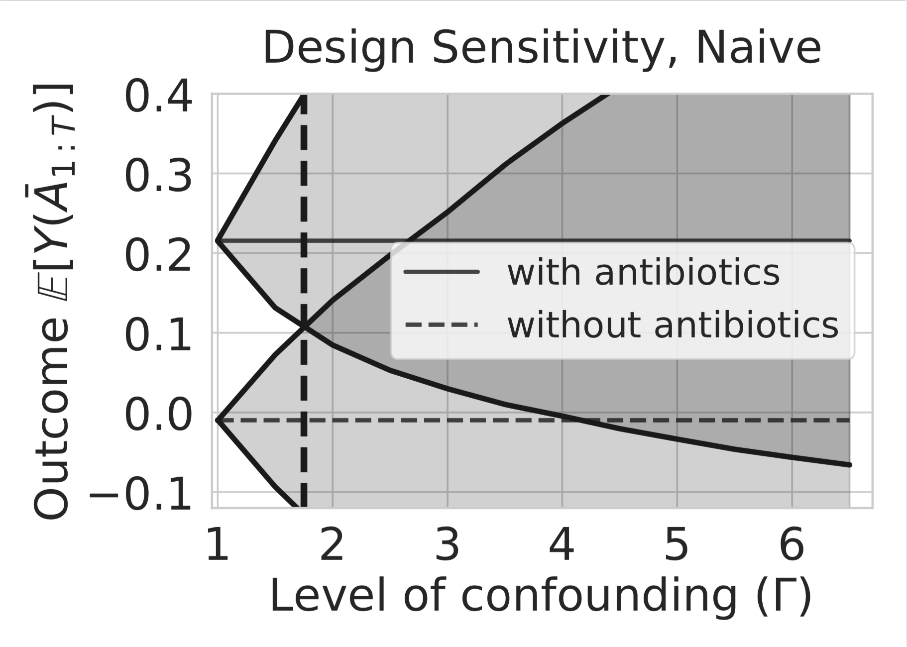
(a) Our approach	(b) Naive approach

Figure 2: Sepsis simulator design sensitivity. Data generation process with level of confounding $\Gamma^{\star}=5$. Estimated lower and upper bound of two policies (with and without antibiotics) under (a) our approach with design sensitivity $5.6$ (b) naive approach with design sensitivity $1.75$.

We illustrate how our approach can generate meaningful certificates of robustness to unobserved confounding in realistic scenarios. We consider selecting evaluation policies using off-policy evaluation methods, such as comparing the expected performance of a new policy to an existing policy. We empirically validate our method in sequential off-policy evaluation problems where confounding is primarily an issue in only a single decision. Since counterfactual outcomes are only known in simulations, we focus on simulated healthcare examples motivated by two real OPE applications: management of sepsis patients, and developmental interventions for autistic children. We select these examples because they represent interesting cases with existing simulators. As we argue shortly, it is plausible to assume that unobserved confounding only affects a single decision in both settings.

The two scenarios characterize different problem regimes. The sepsis simulator models discrete state space and the horizon of decision making ($T$) is naturally multiple steps, and the autism management simulator models continuous-valued states and horizon $T=2$. Our results demonstrate scalability of our loss minimization approach in both discrete and continuous settings, as well as short and medium horizons ($5\sim 10$). We observe that beyond $10$ time steps, overlap becomes a problem, and statistical estimation becomes challenging.

In both examples, we compare three different approaches: standard OPE methods that (incorrectly) assume sequential ignorability, the naïve bound (4), and the bound using our proposed loss minimization approach (7). All the code required to reproduce our experiments are available online at https://github.com/StanfordAI4HI/off_policy_confounding. In both cases our approach provides informative bounds on the performance of the evaluation policy, allowing reliable selection of policies even under unobserved confounding. Compared to the naïve approach (4) which is often prohibitively conservative, our methods allow certifying robustness to much larger levels of confounding $\Gamma$.

6.1 Managing sepsis for ICU patients

As outlined in Section 1.1, automated policies hold much promise in management of sepsis in ICU patients. However, ICU observational data about sepsis patients may often lack information about important confounders, such as important unrecorded comorbidities that affect a clinician’s initial decision whether to administer antibiotics. In subsequent time steps, we assume the (highly-trained) clinical care team follows standard protocols based on vitals signs and lab measurements, and hence their subsequent decisions are unconfounded. On the sepsis simulator developed by Oberst and Sontag (2019), we illustrate how such confounders can bias OPE methods, and demonstrate that our worst-case approach can allow reliable selection of candidate policies under confounding.

We consider a scenario where automated policies have been proposed using existing medical knowledge, and we wish to evaluate their benefits relative to the current standard of care. We evaluate three different policies, all of which only differ in their initial prescription of antibiotics, and otherwise act optimally. The first policy, without antibiotics (WO), does not administer antibiotics initially, whereas the second policy, with antibiotics (W), always administers antibiotics initially. For our last policy, we follow Oberst and Sontag (2019) and use the optimal policy learned by running policy iteration on this simulator—naturally this procedure does not have confounding. We stress that our first two policies are identical to the optimal policy after the initial time step. The true performance of the with antibiotics (W) and optimal policy is quite similar, and better than the without antibiotics (WO) policy (see Figure 1).

To simulate unrecorded comorbidities that could introduce confounding, we extract the randomness that governs state transitions into a confounding variable so that the confounder is correlated with better state transitions. In the first time step, we take the optimal action with respect to all other options (vasopressors and mechanical ventilation), and administer antibiotics with probability $\sqrt{\Gamma^{\star}}/(1+\sqrt{\Gamma^{\star}})$ if the confounding variable is large, and with probability $1/(1+\sqrt{\Gamma^{\star}})$ if the confounding variable is small. This confounder satisfies Assumption E with level $\Gamma^{\star}$. Note that $\Gamma^{\star}$ is used in the data generation process, but is unknown to the procedure used to estimate (bounds on) the evaluation policy performance. We run our method with varying levels of $\Gamma$, and look at thresholds at which the bounds on the performance of evaluation policies cross each other (which we refer to as the design sensitivity).

To generate our observational data, we assume that the care team acts nearly optimally, except for some randomness due to challenges in the ICU; this guarantees overlap (Assumption F) with respect to the optimal evaluation policy. In all but the first time step, we let the behavior policy take the optimal next treatment action with probability $0.85$, and otherwise switch the vasopressor status, independent of the confounders; this guarantees that the assumption of single time step confounding (Assumption D) holds.

Oberst and Sontag (2019)’s simulator state space consists of a binary indicator for diabetes, and four vital signs {heart rate, blood pressure, oxygen concentration and glucose level} that take values in a subset of {very high, high, normal, low, very low}; size of the state space is $|\mathcal{S}_{t}|=1440$. There are three binary treatment options for {antibiotics, vasopressors, and mechanical ventilation}, so that the action space has cardinality $|\mathcal{A}_{t}|=2^{3}$. In our experiments, simulation continues either until at most $T=5$ (horizon) time steps, death (reward -1), or discharge (reward +1). Patients are discharged when all vital signs are in the normal range without treatment. Patients die if at least three vitals are out of the normal range. We refer the reader to https://github.com/clinicalml/gumbel-max-scm for details regarding the simulator.

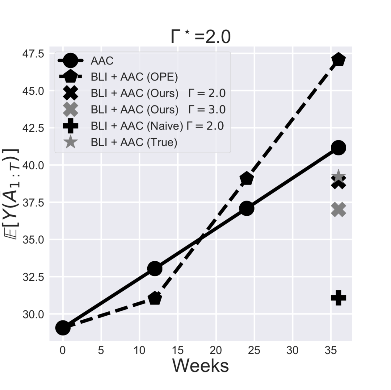
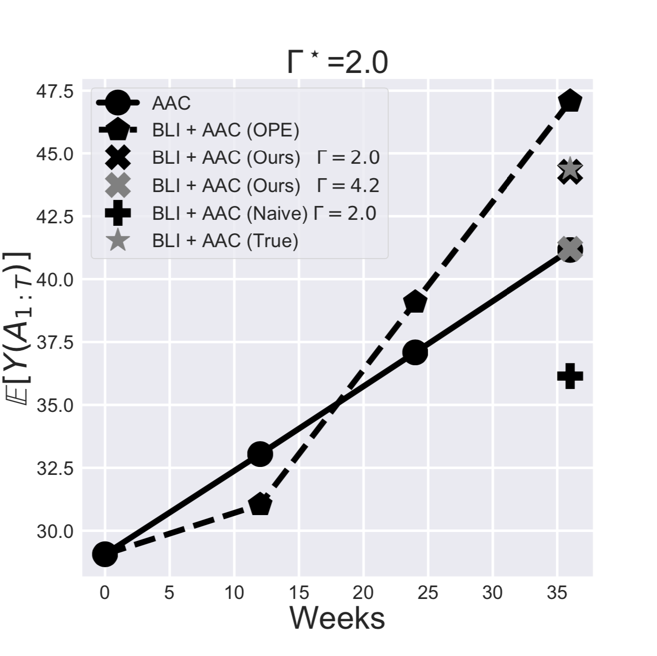
(a) Case I	(b) Case II

Figure 3: Autism simulation. Outcome of two different policies, confounded adaptive policy (BLI+AAC) and un-confounded non-adaptive policy (AAI). Data generation process with the level of confounding $\Gamma^{\star}=2.0$.

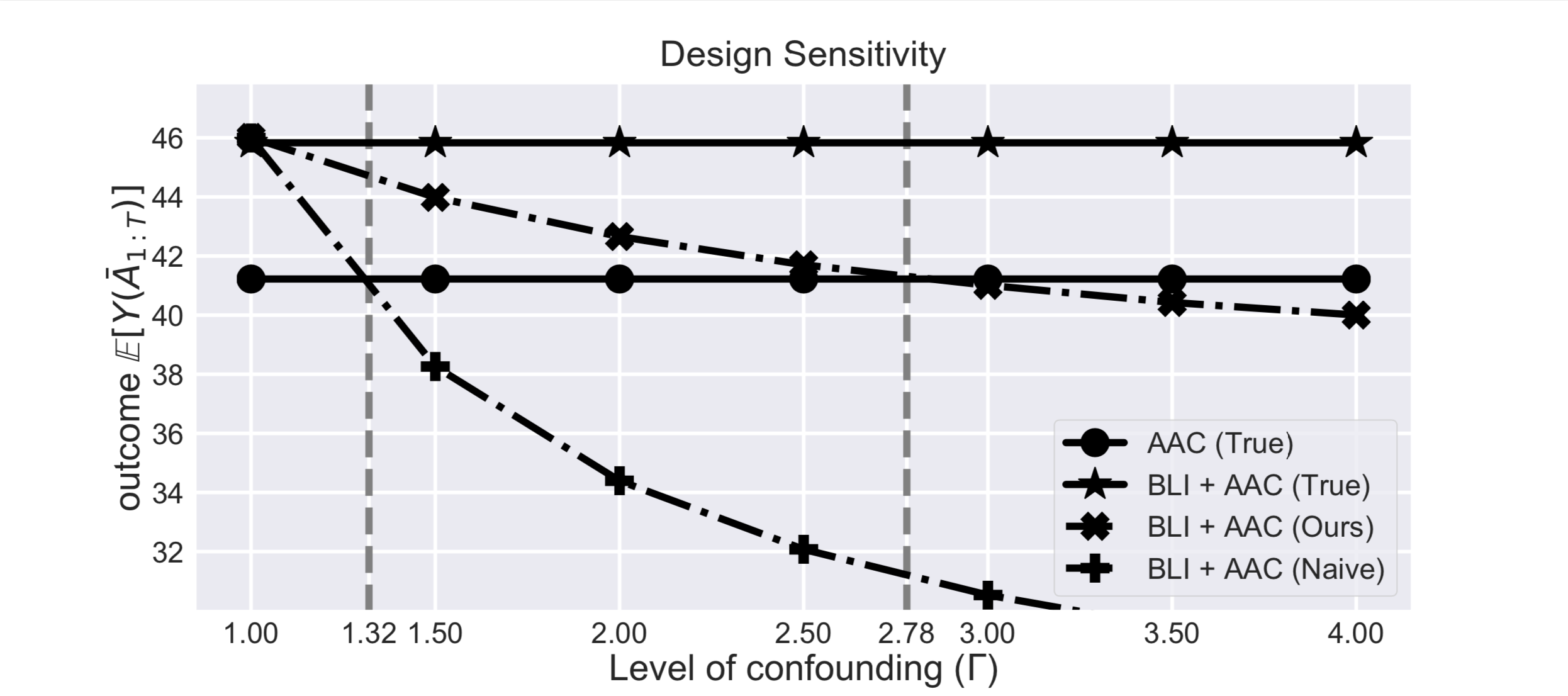
Figure 4: Autism simulation design sensitivity. Data generation process with the level of confounding $\Gamma^{\star}=1.0$. True value of adaptive (BLI+AAC) and non-adaptive (AAC) policies along with estimated lower bound on outcome using our and naive approach

We first consider when our approach happens to use the same confounding degree as what is present in the simulator, $\Gamma=\Gamma^{\star}$. Figure 1 plots the value of the three evaluation decision policies estimated using the data generated with $\Gamma^{\star}=2.0$, which is a fairly small amount of confounding. Confounding leads standard OPE methods that assume sequential ignorability for the behavior policy to underestimate the peformance of the without antibiotics (WO) policy, and overestimate the performance of the with antibiotics (W) and optimal policies. This inflates the expected benefit of the W and optimal policies compared to the WO policy. The naive approach (4) results in very wide estimated intervals over the potential policy performance, and therefore cannot be used to reliably infer the superiority of W and optimal policy over WO even when $\Gamma=2.0$. On the other hand, our proposed method certifies the robustness of the benefit of immediately administering antibiotics; our lower bounds on the performance of the W and optimal policies are better than the upper bound on the performance under the WO policy.

We next consider a much larger amount of confounding, generating the observational data with $\Gamma^{\star}=5.0$. To explore the design sensitivity of our method and our naiïve lower bound approach, we use a range of $\Gamma$ values in our method. Figure 2 shows that for our method, the lower bound on the performance of the W policy meets the upper bound on that of the WO policy at $\Gamma=5.6$. In other words, our approach can reliably estimate that the W policy is better than the WO policy up to assuming an amount of confounding determined by $\Gamma=5.6$ when the true $\Gamma^{\star}=5.0$. In contrast, our proposed naïve bound (4) has a a design sensitivity of $\Gamma=1.75$, meaning the bounds quickly fails to be informative far below the true amount of data confounding. Our method allow concluding that the W policy is superior to the WO policy even when a substantial amount of unobserved confounding exists in the initial decision.

6.2 Communication interventions for minimally verbal children with autism

We next consider another motivating scenario from healthcare, but one which naturally involves continuous variables to demonstrate that our approach is also able to compute reasonable lower bounds for such a case, while using function approximation.

Minimally verbal children represent 25-30% of children with autism, and often have poor prognosis in terms of social functioning (Rutter et al., 1967; Anderson et al., 2009). We are interested in comparing non-adaptive versus adaptive approaches that aim to improve spoken communication, measured by the number of speech utterances. We introduce confounding using a simulator for autistic children developed by Lu et al. (2016), which models the data from a (real) sequential, multiple assignment, randomized trial (SMART) (Kasari et al., 2014). Despite their randomized trial, Kasari et al. (2014) note that very few randomized trials of these interventions exist, and the number of individuals in these trials tends to be small. It is therefore reasonable to think that in similar settings it would be beneficial to use existing off-policy data to evaluate new intervention protocols.

In the simulator there are two developmental interventions (actions): behavioral language interventions (BLI) delivered by a therapist, and an augmented/alternative communication (AAC) approach implemented with a speech generation device. There are two decision points in the data generation process: week 0 and week 12. Number of speech utterances are measured at week 0, 12, 24 and 36: note that the action / intervention applied at week 12 persists from week 12 to the end of the process, which means this is a 2 time step decision problem. Here the outcome is modeled as a continuous variable representing the average number of speech utterances for a given patient.

We consider a scenario where participants were recruited and randomly assigned to the two treatment options initially (i.e., $A_{1}\sim\mbox{Unif}(\left\{\mbox{BLI},\mbox{AAC}\right\})$), and a recourse action is taken after a follow-up visit after 12 weeks. Depending on the progress of patients at Week 12, the clinician decides whether to switch to AAC devices for children who started with BLI. Since this intervention requires a specialized device—whose supply is limited—it is likely that the clinicians assign AAC devices for whom it has a higher chance of being effective. Such subjective assessments are likely based on the their interaction with patients that contain partial, noisy information about the final outcome, which are often not recorded properly. Therefore, while there is confounding in the second decision ($t^{\star}=2$), its influence may be appropriately bounded (i.e., Assumption D is plausible). To simulate confounding, we expand the simulator to create variables that partially influences the effectiveness of switching from BLI to AAC, and use knowledge of this to alter the behavior policy decisions at Week 12. The resulting confounding satisfies our model of bounded confounding (Assumption D) and is described in detail in Appendix D.2.

In our evaluations, we compare an adaptive policy (BLI + AAC) that starts with BLI, and augments BLI with AAC at week 12 if the patient is a slow responder, against a non-adaptive policy that uses AAC through the whole treatment. We simulate two different settings where the effect of switching to the AAC treatment varies; our simulation parameters are within the suggested range of  Lu et al. (2016)’s recommendations based on the SMART trial data. We note that OPE estimates for the non-adaptive policy (AAC) is unbiased since observations for this outcome are unconfounded. Our loss minimization for computing the lower bound using $\kappa(a_{t^{\star}},H_{t^{\star}})$ is done using a 4 layers neural network with Relu activations, we use backpropogation with AdamOptimizer and weighted squared loss given in Theorem 2. We use logistic regression to estimate the behavior policy, note that this is the marginalized behavior policy since the latent confounder is unobserved.

In Case I, we define the parameters such that the adaptive policy (BLI+AAC) is worse the non-adaptive policy (AAC) (lower true outcome / performance). As shown in Figure 3 (a), standard OPE approach overestimates the outcome of the adaptive policy even given a mild level of confounding $\Gamma^{\star}=2.0$, and would incorrectly suggest the BLI+AAC policy outperforms the AAC policy. On the other hand, our lower bounds on the adaptive policy computed using $\Gamma=2$ (recall the true confounding amount is unknown to our approach) suggest the OPE estimates may be biased enough to affect conclusions; the observed advantages of the adaptive policy may be attributed solely to unobserved confounding, even under reasonable values of confounding ($\Gamma=2$).

In Case II, we change the parameters so that the BLI+AAC policy is better than the AAC policy, and again use a true amount of confounding of $\Gamma^{\star}=2.0$ in the data generation process. Standard OPE estimates again overestimate the outcome for the BLI+AAC policy (Figure 3(b)). The naïve lower bound results in a conservative lower bound that would again indicate no conclusions can be drawn about the relative performance of BLI+AAC versus AAC. However, our method can certify the superiority of the BLI+AAC policy when the level of confounding used in the computation of the lower bounds is up to $\Gamma=4.2$, thereby providing a case where our approach can provide useful certificates of benefit of a new decision policy under non-trivial levels of confounding.

Figure 4 plots the design sensitivity of our method against the naïve approach (4), when there is in fact no confounding in the data generation process ($\Gamma^{\star}=1$). Compared to the naive approach (design sensitivity is $\Gamma=1.32$), our method allows certifying robustness of the finding—that the adaptive policy is advantageous—up to realistic levels of confounding (design sensitivity is $\Gamma=2.78$).

7 Discussion

In this work, we proposed methods for analyzing the sensitivity of OPE methods to unobserved confounding in sequential decision making problems. We demonstrated how our approach can certify robustness of OPE in some settings, or raise concerns about its validity based on sensitivity to unobserved confounding. Our loss minimization method allows computing worst-case bounds over our bounded unobserved confounding model, while adjusting for observed features via importance sampling.

As a consequence, our estimators face the same challenges that standard importance-sampling-based OPE methods face: high variance when there is little overlap between the evaluation and behavior policy. In our experiments, importance sampling was effective since we ensured that there was sufficient overlap and focused on shorter horizons. In other settings, lack of overlap poses fundamental difficulties in off policy evaluation, beyond issues with confounding, as others have also noted (Gottesman et al., 2019a). Such challenges become pronounced as the horizon $T$ or the importance sampling weights (1) become large. While stationary importance sampling (SIS) can reduce variance, rewards under stationary distributions (should they exist) are not appropriate for the problems studied in this paper; SIS (Hallak and Mannor, 2017; Liu et al., 2018a; Xie et al., 2019; Liu et al., 2019) nevertheless still suffers high variance when there is a lack of overlap. Fujimoto et al. (2019) and Kumar et al. (2019) suggest some promising algorithmic approaches for only considering (and optimizing over) policies with sufficient overlap: while more work is needed, policies generated by these approaches would be more amenable to OPE, and should improve the statistical properties of our method.

It is natural to consider extending our single-decision confounding model to settings where a handful of decisions (say 2-5) are affected by unobserved confounding. Worst-case bounds on $\mathbb{E}[Y(\bar{A}_{1:T})]$ under such extensions require solving optimization problems involving products of likelihood ratios defined over different confounded time periods. Since these problems are nonconvex, they require new approaches than the one we take here, which heavily depends on applying convex duality.

Appendix A Proof of basic lemmas

Before we give the proof of our main results, we give a set of essentially standard lemmas that we build on in the rest of the paper. In the following, we use a notational shorthand for (nested) expectations under observable distributions: for all $1\leq t\leq T$ and $1\leq t_{1}\leq t_{2}\leq T$,

$$\mathbb{E}^{t}_{a_{t}}[X]:=\mathbb{E}[X\mid H_{t},A_{t}=a_{t}]~{}~{}~{}\mbox{and}~{}$$ (8a)

$$\mathbb{E}^{t_{1}:t_{2}}_{a_{t_{1}:t_{2}}}[X]:=\mathbb{E}^{t_{1}}_{a_{t_{1}}}[\mathbb{E}^{t_{1}+1}_{a_{t_{1}+1}}[\cdots\mathbb{E}^{t_{2}}_{a_{t_{2}}}[X]\cdots]].$$ (8b)

Similarly, we write for all $1\leq t_{0}\leq t_{1}\leq t_{2}\leq T$

$$\mathbb{E}^{t_{2}}_{a_{t_{1}:t_{2}}}[X]:=\mathbb{E}[X\mid H_{t}(A_{1:t_{1}-1},a_{t_{1}:t_{2}-1}),A_{t_{2}}=a_{t_{2}}]~{}~{}~{}\mbox{and}~{}$$ (9a)

$$\mathbb{E}^{t_{1}:t_{2}}_{a_{t_{0}:t_{2}}}[X]:=\mathbb{E}^{t_{1}}_{a_{t_{0}:t_{1}}}[\mathbb{E}^{t_{1}+1}_{a_{t_{0}:t_{1}+1}}[\cdots\mathbb{E}^{t_{2}}_{a_{t_{0}:t_{2}}}[X]\cdots]].$$ (9b)

The cumulative rewards $\mathbb{E}[Y(\bar{A}_{1:T})]$ under the candidate policy has an alternate representation, which we draw on heavily in the rest of the proofs. See Section A.1 for a derivation.

Lemma 4.

If sequential ignorability (Assumption A) holds for the evaluation policy $\bar{\pi}$, we have the identity

$$\mathbb{E}\left[Y(\bar{A}_{1:T})\right]=\sum_{a_{1:T}}\mathbb{E}\left[Y(a_{1:T})\prod_{t=1}^{T}\bar{\pi}_{t}(a_{t}\mid\bar{H}_{t}(a_{1:t-1}))\right].$$

To ease notation, denote each integrand in the above sum by

$$Y(a_{1:T};\bar{\pi}):=Y(a_{1:T})\prod_{t=1}^{T}\bar{\pi}_{t}(a_{t}\mid\bar{H}_{t}(a_{1:t-1})).$$ (10)

We will also use the following two identities heavily. Recall that we denote by $W:=\{W(a_{1:T})\}_{a_{1:T}}$, the tuple of all potential outcomes, which takes values in $\mathcal{W}$. See Section A.2 for a proof of the following result.

Lemma 5.

Let sequential ignorability (Assumption A) hold for the behavioral policy $\pi$ in the time steps $t_{1}:t_{2}$, where $1\leq t_{1}<t_{2}\leq T$. Then, for any measurable $f:\mathcal{W}\to\mathbb{R}$

$$\mathbb{E}[f(W)\mid H_{t_{1}}(a_{1:t_{1}-1})]=\mathbb{E}\left[\mathbb{E}_{a_{1:t_{2}}}^{t_{1}:t_{2}}\left[f(W)\right]\mid H_{t_{1}}(a_{1:t_{1}-1})\right]$$

for any $a_{1:t_{2}}\in\mathcal{A}_{1}\times\cdots\times\mathcal{A}_{t_{2}}$.

The following identity—whose proof we give in Section A.3—is a simple consequence of the definition of conditional expectations, and the tower law.

Lemma 6.

For any measurable function $f:\mathcal{W}\to\mathbb{R}$, and $1\leq t_{1}\leq t_{2}\leq T$,

$$\mathbb{E}_{a_{1:t_{2}}}^{t_{1}:t_{2}}f(W)=\mathbb{E}\left[f(W)\prod_{t=t_{1}}^{t_{2}}\frac{\mathbf{1}\left\{A_{T}=a_{t}\right\}}{\pi_{t}(a_{t}\mid H_{t}(a_{1:t-1}))}\mid H_{t_{1}}(a_{1:t_{1}-1})\right]$$

A.1 Proof of Lemma 4

Similar to the notational shorthand (8), define

$$\overline{\mathbb{E}}^{t}_{a_{1:t}}[X]:=\mathbb{E}[X\mid\bar{H}_{t}(a_{1:t-1}),\bar{A}_{t}=a_{t}]~{}~{}~{}\mbox{and}~{}~{}~{}\overline{\mathbb{E}}^{t:T}_{a_{1:T}}[X]=\overline{\mathbb{E}}^{t}_{a_{1:t}}[\overline{\mathbb{E}}^{t+1}_{a_{1:t+1}}[\cdots\overline{\mathbb{E}}^{T}_{a_{1:T}}[X]\cdots]].$$

Begin by noting that by definition of conditional expectation

$$\mathbb{E}[Y(\bar{A}_{1:T})\mid\bar{H}_{1}] =\sum_{a_{1}\in\mathcal{A}_{1}}\bar{\pi}(a_{1}\mid\bar{H}_{1})\mathbb{E}[Y(a_{1},\bar{A}_{2:T})\mid\bar{H}_{1},\bar{A}_{1}=a_{1}]$$

$$=\sum_{a_{1}\in\mathcal{A}_{1}}\bar{\pi}(a_{1}\mid\bar{H}_{1})\overline{\mathbb{E}}^{1}_{a_{1}}[Y(a_{1},\bar{A}_{2:T})],$$

and similarly, conditioning on $\bar{H}_{2}(a_{1})=(S_{1},\bar{A}_{1}=a_{1},S_{2}(a_{1}))$ yields

$$\mathbb{E}[Y(a_{1},\bar{A}_{2:T})\mid\bar{H}_{2}(a_{1})] =\sum_{a_{2}\in\mathcal{A}_{2}}\bar{\pi}_{2}(a_{2}\mid\bar{H}_{2}(a_{1}))\mathbb{E}[Y(a_{1:2},\bar{A}_{3:T})\mid\bar{H}_{2}(a_{1}),\bar{A}_{2}=a_{2}]$$

$$=\sum_{a_{2}\in\mathcal{A}_{2}}\bar{\pi}_{2}(a_{2}\mid\bar{H}_{2}(a_{1}))\overline{\mathbb{E}}^{2}_{a_{1:2}}[Y(a_{1:2},\bar{A}_{3:T})].$$

From the tower law, the above two equalities yield

$$\mathbb{E}[Y(\bar{A}_{1:T})] =\mathbb{E}\Bigg{[}\sum_{a_{1}\in\mathcal{A}_{1}}\bar{\pi}_{1}(a_{1}\mid\bar{H}_{1})\mathbb{E}\Bigg{[}\sum_{a_{2}\in\mathcal{A}}\bar{\pi}_{2}(a_{2}\mid\bar{H}_{2}(a_{1}))\cdot\mathbb{E}[Y(a_{1:2},\bar{A}_{3:T})\mid\bar{H}_{2}(a_{1}),\bar{A}_{2}=a_{2}]\Bigg{|}\bar{H}_{1},\bar{A}_{1}=a_{1}\Bigg{]}\Bigg{]}$$

$$=\mathbb{E}\Bigg{[}\sum_{a_{1}\in\mathcal{A}_{1}}\bar{\pi}_{1}(a_{1}\mid\bar{H}_{1})\overline{\mathbb{E}}^{1}_{a_{1}}\Bigg{[}\sum_{a_{2}\in\mathcal{A}}\bar{\pi}_{2}(a_{2}\mid\bar{H}_{2}(a_{1}))\cdot\overline{\mathbb{E}}^{2}_{a_{1:2}}[Y(a_{1:2},\bar{A}_{3:T})]\Bigg{]}\Bigg{]}.$$

Proceeding iteratively as before and expanding each $\mathbb{E}[Y(a_{1:t-1},\bar{A}_{t:T})\mid\bar{H}_{t}(a_{1:t-1})]$, we arrive at

$$\mathbb{E}[Y(\bar{A}_{1:T})]$$

$$=\mathbb{E}\left[\sum_{a_{1}\in\mathcal{A}_{1}}\bar{\pi}_{1}(a_{1}\mid\bar{H}_{1})\overline{\mathbb{E}}^{1}_{a_{1}}\left[\overline{\mathbb{E}}^{2}_{a_{1:2}}\left[\sum_{a_{2}\in\mathcal{A}_{2}}\bar{\pi}_{2}(a_{2}\mid\bar{H}_{2}(a_{1}))\overline{\mathbb{E}}^{3}_{a_{1:3}}\left[\cdots\sum_{a_{T}\in\mathcal{A}_{T}}\bar{\pi}_{T}(a_{T}\mid\bar{H}_{T}(a_{1:T-1}))\overline{\mathbb{E}}^{T}_{a_{1:T}}\left[Y(a_{1:T})\right]\right]\right]\right]\right].$$

Now, we proceed backwards from the inner most expectation to take the outer sum inside the expectation. By Assumption A, we have

$$\sum_{a_{T}\in\mathcal{A}_{T}}\bar{\pi}_{T}(a_{T}\mid\bar{H}_{T}(a_{1:T-1}))\overline{\mathbb{E}}^{T}_{a_{1:T}}\left[Y(a_{1:T})\right] =\sum_{a_{T}\in\mathcal{A}_{T}}\bar{\pi}_{T}(a_{T}\mid\bar{H}_{T}(a_{1:T-1}))\cdot\mathbb{E}\left[Y(a_{1:T})~{}\Bigg{|}~{}\bar{H}_{T}(a_{1:T-1})\right]$$

$$=\mathbb{E}\left[\sum_{a_{T}\in\mathcal{A}_{T}}\bar{\pi}_{T}(a_{T}\mid\bar{H}_{T}(a_{1:T-1}))\cdot Y(a_{1:T})~{}\bigg{|}~{}\bar{H}_{T}(a_{1:T-1})\right].$$

Noting that $\mathbb{E}[\cdot~{}|~{}\bar{H}_{T}(a_{1:T-1})]=\mathbb{E}[\cdot~{}|~{}\bar{H}_{T-1}(a_{1:T-2}),S_{T}(a_{1:T-1}),\bar{A}_{T-1}{=}a_{T-1}]$, the tower law and preceding display yield

$$\overline{\mathbb{E}}^{T-1}_{a_{1:T-1}}\left[\sum_{a_{T}\in\mathcal{A}_{T}}\bar{\pi}_{T}(a_{T}\mid\bar{H}_{T}(a_{1:T-1}))\cdot\overline{\mathbb{E}}^{T}_{a_{1:T}}\left[Y(a_{1:T})\right]\right]=\overline{\mathbb{E}}^{T-1}_{a_{1:T-1}}\left[\sum_{a_{T}\in\mathcal{A}_{T}}\bar{\pi}_{T}(a_{T}\mid\bar{H}_{T}(a_{1:T-1}))\cdot Y(a_{1:T})\right].$$

We repeat an identical process for the sum over $a_{T-1}$. Similarly as above, applying Assumption A gives

$$\sum_{a_{T-1}\in\mathcal{A}_{T-1}}\bar{\pi}_{T-1}(a_{T-1}\mid\bar{H}_{T-1}(a_{1:T-2}))\cdot\overline{\mathbb{E}}^{T-1}_{a_{1:T-1}}\left[\sum_{a_{T}\in\mathcal{A}_{T}}\bar{\pi}_{T}(a_{T}\mid\bar{H}_{T}(a_{1:T-1}))\cdot Y(a_{1:T})\right]$$

$$=\mathbb{E}\left[\sum_{a_{T-1}\in\mathcal{A}_{T-1}}\bar{\pi}_{T-1}(a_{T-1}\mid\bar{H}_{T-1}(a_{1:T-2}))\sum_{a_{T}\in\mathcal{A}_{T}}\bar{\pi}_{T}(a_{T}\mid\bar{H}_{T}(a_{1:T-1}))\cdot Y(a_{1:T})~{}\bigg{|}~{}\bar{H}_{T-1}(a_{1:T-2})\right].$$

By the tower law, we again get

$$\overline{\mathbb{E}}^{T-2}_{a_{1:T-2}}\left[\sum_{a_{T-1}\in\mathcal{A}_{T-1}}\bar{\pi}_{T-1}(a_{T-1}\mid\bar{H}_{T-1}(a_{1:T-2}))\overline{\mathbb{E}}^{T-1}_{a_{1:T-1}}\left[\sum_{a_{T}\in\mathcal{A}_{T}}\bar{\pi}_{T}(a_{T}\mid\bar{H}_{T}(a_{1:T-1}))\cdot Y(a_{1:T})\right]\right]$$

$$=\overline{\mathbb{E}}^{T-2}_{a_{1:T-2}}\left[\sum_{a_{T-1}\in\mathcal{A}_{T-1}}\bar{\pi}_{T-1}(a_{T-1}\mid\bar{H}_{T-1}(a_{1:T-2}))\cdot\sum_{a_{T}\in\mathcal{A}_{T}}\bar{\pi}_{T}(a_{T}\mid\bar{H}_{T}(a_{1:T-1}))\cdot Y(a_{1:T})\right].$$

Iterating the above process over the indices $t=T-2,\ldots,1$, we arrive at the desired formula.

A.2 Proof of Lemma 5

From the tower law and sequential ignorability of $\pi$,

$$\mathbb{E}[f(W)\mid H_{t_{1}}(a_{1:t_{1}-1})] =\mathbb{E}[f(W)\mid H_{t_{1}}(a_{1:t_{1}-1}),A_{t_{1}}=a_{t_{1}}]$$

$$=\mathbb{E}[\mathbb{E}[f(W)\mid H_{t_{1}+1}(a_{1:t_{1}})]\mid H_{t_{1}}(a_{1:t_{1}-1}),A_{t_{1}}=a_{t_{1}}]$$

Applying the tower law to the inner expectation, and applying sequential ignorability again, we get

$$\mathbb{E}[f(W)\mid H_{t_{1}+1}(a_{1:t_{1}})]=\mathbb{E}\left[\mathbb{E}[f(W)\mid H_{t_{1}+2}(a_{1:t_{1}+1})]\mid H_{t_{1}+1}(a_{1:t_{1}}),A_{t_{1}+1}=a_{t_{1}+1}\right]$$

Plugging this back into the original display, we have

$$\mathbb{E}[f(W)\mid H_{t_{1}}(a_{1:t_{1}-1})]=\mathbb{E}_{a_{1}:t_{1}+1}^{t_{1}:t_{1}+1}\left[\mathbb{E}[f(W)\mid H_{t_{1}+2}(a_{1:t_{1}+1})]\right]$$

Repeating this argument over $t=t_{1}+2,\ldots,t_{2}$, we conclude the result.

A.3 Proof of Lemma 6

From the definition of conditional expectations, we have

$$\mathbb{E}[f(W)\mid H_{t}(a_{1:t-1}),A_{t}=a_{t}]=\mathbb{E}\left[f(W)\frac{\mathbf{1}\left\{A_{t}=a_{t}\right\}}{\pi_{t}(a_{t}\mid H_{t}(a_{1:t-1}))}\mid H_{t}(a_{1:t-1})\right].$$

The result follows by applying this equality at $t=t_{2}$, applying the tower law, and iterating the same argument over $t=t_{2}-1,\ldots,t_{1}$.

Appendix B Proof of key identities

B.1 Proof of Lemma 1

Recalling the notation (10), sequential ignorability of $\bar{\pi}$ and Lemma 4 gives the following representation

$$\mathbb{E}\left[Y(\bar{A}_{1:T})\right]=\sum_{a_{1:T}}\mathbb{E}\left[Y(a_{1:T};\bar{\pi})\right].$$

We deal with each term $\mathbb{E}[Y(a_{1:T};\bar{\pi})]$ in the summation separately, for each fixed sequence of actions $a_{1:T}$. From sequential ignorability of $\pi$ and Lemma 5,

$$\mathbb{E}[Y(a_{1:T};\bar{\pi})]=\mathbb{E}[\mathbb{E}^{1}_{a_{1}}[\cdots\mathbb{E}^{T}_{a_{1:T}}[Y(a_{1:T};\bar{\pi})]\cdots]]=\mathbb{E}[\mathbb{E}^{1:T}_{a_{1:T}}[Y(a_{1:T};\bar{\pi})]].$$

Applying Lemma 6, we get

$$\mathbb{E}[Y(a_{1:T};\bar{\pi})]=\mathbb{E}[Y(a_{1:T};\bar{\pi})\prod_{t=1}^{T}\frac{\mathbf{1}\left\{A_{t}=a_{t}\right\}}{\pi_{t}(a_{t}\mid H_{t}(a_{1:t-1}))}].$$

Summing the preceeding display over $a_{1:T}$, we obtain the desired result.

B.2 Proof of Proposition 1

From Lemma 4, we have

$$\mathbb{E}[Y(\bar{A}_{1:T})]=\mathbb{E}\left[\sum_{a_{1:T}}Y(a_{1:T})\prod_{t=1}^{T}\bar{\pi}_{t}(a_{t}\mid\bar{H}_{t}(a_{1:t-1}))\right].$$

Since sequential ignorability for $\pi$ holds at any $t<t^{\star}$, Lemma 5 implies that the preceeding display is equal to

$$\mathbb{E}\left[\sum_{a_{1:t^{\star}-1}}\mathbb{E}_{a_{1:t^{\star}-1}}^{1:t^{\star}-1}\left[\sum_{a_{t^{\star}:T}}Y(a_{1:T})\prod_{t=1}^{T}\bar{\pi}_{t}(a_{t}\mid\bar{H}_{t}(a_{1:t-1}))\right]\right].$$

Applying Lemma 6 to the inner expectations, we get

$$\mathbb{E}[Y(\bar{A}_{1:T})] =\mathbb{E}\left[\sum_{a_{1:t^{\star}-1}}\prod_{t=1}^{t^{\star}-1}\frac{\mathbf{1}\left\{A_{t}=a_{t}\right\}}{\pi_{t}(a_{t}\mid H_{t}(a_{1:t-1}))}\sum_{a_{t^{\star}:T}}Y(a_{1:T})\prod_{t=1}^{T}\bar{\pi}_{t}(a_{t}\mid\bar{H}_{t}(a_{1:t-1}))\right]$$

$$=\mathbb{E}\left[\prod_{t=1}^{t^{\star}-1}\frac{\bar{\pi}_{t}(A_{t}\mid\bar{H}_{t}(A_{1:t-1}))}{\pi_{t}(A_{t}\mid H_{t})}\sum_{a_{t^{\star}:T}}Y(A_{1:t^{\star}-1},a_{t^{\star}:T})\prod_{t=t^{\star}}^{T}\bar{\pi}_{t}(a_{t}\mid\bar{H}_{t}(A_{1:t^{\star}-1},a_{t^{\star}:t-1}))\right].$$

From the tower law, we arrive at

$$\mathbb{E}[Y(\bar{A}_{1:T})] =\mathbb{E}\left[\mathbb{E}\left[\prod_{t=1}^{t^{\star}-1}\frac{\bar{\pi}_{t}(A_{t}\mid\bar{H}_{t}(A_{1:t-1}))}{\pi_{t}(A_{t}\mid H_{t})}\sum_{a_{t^{\star}:T}}Y(A_{1:t^{\star}-1},a_{t^{\star}:T})\prod_{t=t^{\star}}^{T}\bar{\pi}_{t}(a_{t}\mid\bar{H}_{t}(A_{1:t^{\star}-1},a_{t^{\star}:t-1}))~{}\Bigg{|}~{}H_{t^{\star}}\right]\right]$$

$$=\mathbb{E}\left[\prod_{t=1}^{t^{\star}-1}\frac{\bar{\pi}_{t}(A_{t}\mid\bar{H}_{t}(A_{1:t-1}))}{\pi_{t}(A_{t}\mid H_{t})}\mathbb{E}\left[\sum_{a_{t^{\star}:T}}Y(A_{1:t^{\star}-1},a_{t^{\star}:T})\prod_{t=t^{\star}}^{T}\bar{\pi}_{t}(a_{t}\mid\bar{H}_{t}(A_{1:t^{\star}-1},a_{t^{\star}:t-1}))~{}\Bigg{|}~{}H_{t^{\star}}\right]\right].$$ (12)

Applying the tower law to the inner expectation in the final display, we can write

$$\mathbb{E}\left[\sum_{a_{t^{\star}:T}}Y(A_{1:t^{\star}-1},a_{t^{\star}:T})\prod_{t=t^{\star}}^{T}\bar{\pi}_{t}(a_{t}\mid\bar{H}_{t}(A_{1:t^{\star}-1},a_{t^{\star}:t-1}))~{}\Bigg{|}~{}H_{t^{\star}}\right]$$

$$=\mathbb{E}\left[\mathbb{E}\left[\sum_{a_{t^{\star}:T}}Y(A_{1:t^{\star}-1},a_{t^{\star}:T})\prod_{t=t^{\star}}^{T}\bar{\pi}_{t}(a_{t}\mid\bar{H}_{t}(A_{1:t^{\star}-1},a_{t^{\star}:t-1}))~{}\Bigg{|}~{}H_{t^{\star}},A_{t^{\star}}\right]~{}\Bigg{|}~{}H_{t^{\star}}\right]$$

$$=\sum_{a_{t^{\star}},a_{t^{\star}}^{\prime}}\bar{\pi}_{t^{\star}}(a_{t^{\star}}\mid\bar{H}_{t^{\star}}(A_{1:t^{\star}-1}))\pi_{t^{\star}}(a_{t^{\star}}^{\prime}\mid H_{t^{\star}})$$

$$\qquad\qquad\times\mathbb{E}\left[\sum_{a_{t^{\star}+1:T}}Y(A_{1:t^{\star}-1},a_{t^{\star}:T})\prod_{t=t^{\star}+1}^{T}\bar{\pi}_{t}(a_{t}\mid\bar{H}_{t}(A_{1:t^{\star}-1},a_{t^{\star}:t-1}))~{}\Bigg{|}~{}H_{t^{\star}},A_{t^{\star}}=a_{t^{\star}}^{\prime}\right]$$

$$=\sum_{a_{t^{\star}},a_{t^{\star}}^{\prime}}\bar{\pi}_{t^{\star}}(a_{t^{\star}}\mid\bar{H}_{t^{\star}}(A_{1:t^{\star}-1}))\pi_{t^{\star}}(a_{t^{\star}}^{\prime}\mid H_{t^{\star}})$$

$$\qquad\qquad\times\mathbb{E}\left[\mathcal{L}(W;H_{t^{\star}},a_{t^{\star}},a_{t^{\star}}^{\prime})\sum_{a_{t^{\star}+1:T}}Y(A_{1:t^{\star}-1},a_{t^{\star}:T})\prod_{t=t^{\star}+1}^{T}\bar{\pi}_{t}(a_{t}\mid\bar{H}_{t}(A_{1:t^{\star}-1},a_{t^{\star}:t-1}))~{}\Bigg{|}~{}H_{t^{\star}},A_{t^{\star}}=a_{t^{\star}}\right]$$

where in the last equality, we used the definition

$$\mathcal{L}(\cdot;H_{t^{\star}},a_{t^{\star}},a_{t^{\star}}^{\prime}):=\frac{dP_{W}(\cdot\mid H_{t^{\star}},A_{t^{\star}}=a_{t^{\star}}^{\prime})}{dP_{W}(\cdot\mid H_{t^{\star}},A_{t^{\star}}=a_{t^{\star}})}.$$

Again, by the tower law,

$$\mathbb{E}\left[\mathcal{L}(W;H_{t^{\star}},a_{t^{\star}},a_{t^{\star}}^{\prime})\sum_{a_{t^{\star}+1:T}}Y(A_{1:t^{\star}-1},a_{t^{\star}:T})\prod_{t=t^{\star}+1}^{T}\bar{\pi}_{t}(a_{t}\mid\bar{H}_{t}(A_{1:t^{\star}-1},a_{t^{\star}:t-1}))~{}\Bigg{|}~{}H_{t^{\star}},A_{t^{\star}}=a_{t^{\star}}\right]$$

$$=\mathbb{E}\Bigg{[}\mathbb{E}\Big{[}\mathcal{L}(W;H_{t^{\star}},a_{t^{\star}},a_{t^{\star}}^{\prime})\sum_{a_{t^{\star}+1:T}}Y(A_{1:t^{\star}-1},a_{t^{\star}:T})$$

$$\qquad\qquad\qquad\qquad\times\prod_{t=t^{\star}+1}^{T}\bar{\pi}_{t}(a_{t}\mid\bar{H}_{t}(A_{1:t^{\star}-1},a_{t^{\star}:t-1}))\Big{|}H_{t^{\star}+1}(A_{1:t^{\star}-1},a_{t^{\star}})\Big{]}~{}\Bigg{|}~{}H_{t^{\star}},A_{t^{\star}}=a_{t^{\star}}\Bigg{]}$$

From sequential ignorability of $\pi$ for $t>t^{\star}$ and Lemma 5, the preceeding display is equal to

$$\mathbb{E}\left[\sum_{a_{t^{\star}+1:T}}\mathbb{E}_{a_{t^{\star}:T}}^{t^{\star}+1:T}\mathcal{L}(W;H_{t^{\star}},a_{t^{\star}},a_{t^{\star}}^{\prime})Y(A_{1:t^{\star}-1},a_{t^{\star}:T})\prod_{t=t^{\star}+1}^{T}\bar{\pi}_{t}(a_{t}\mid\bar{H}_{t}(A_{1:t^{\star}-1},a_{t^{\star}:t-1}))~{}\Bigg{|}~{}H_{t^{\star}},A_{t^{\star}}=a_{t^{\star}}\right].$$

From Lemma 6, we can rewrite the above expression as

$$\mathbb{E}\left[\mathcal{L}(W;H_{t^{\star}},a_{t^{\star}},a_{t^{\star}}^{\prime})Y_{t^{\star}}(a_{t^{\star}})\prod_{t=t^{\star}+1}^{T}\frac{\bar{\pi}_{t}(A_{t}\mid\bar{H}_{t}(A_{1:t^{\star}-1},a_{t^{\star}},A_{t^{\star}+1:t}))}{\pi_{t}(A_{t}\mid H_{t}(A_{1:t^{\star}-1},a_{t^{\star}},A_{t^{\star}+1:t}))}~{}\Bigg{|}~{}H_{t^{\star}},A_{t^{\star}}=a_{t^{\star}}\right].$$

Plugging these expressions back into the equality (12), we obtain the result.

Appendix C Proof of bounds under unobserved confounding

C.1 Naive bound

We show the below more general result.

Lemma 7.

Let Assumptions A, B, C hold. Then, we have

$$\mathbb{E}[Y(\bar{A}_{1:T})]\geq\mathbb{E}\left[Y(A_{1:T})\prod_{t=1}^{T}\frac{\bar{\pi}_{t}(A_{t}\mid\bar{H}_{t}(A_{1:t-1}))}{\pi_{t}(A_{t}\mid H_{t})(\Gamma_{t}^{-1}\mathbf{1}\left\{Y(A_{1:T})<0\right\}+\Gamma_{t}\mathbf{1}\left\{Y(A_{1:T})>0\right\})}\right].$$

Proof of Lemma    From an identical argument as the proof of Lemma 1, Assumption B yields

$$\mathbb{E}[Y(\bar{A}_{1:T})]=\mathbb{E}\left[Y(A_{1:T})\prod_{t=1}^{T}\frac{\bar{\pi}_{t}(A_{t}\mid\bar{H}_{t}(A_{1:t-1}),U_{t})}{\pi_{t}(A_{t}\mid H_{t},U_{t})}\right].$$

From Assumption A, the preceeding display is equal to

$$\mathbb{E}[Y(\bar{A}_{1:T})]=\mathbb{E}\left[Y(A_{1:T})\prod_{t=1}^{T}\frac{\bar{\pi}_{t}(A_{t}\mid\bar{H}_{t}(A_{1:t-1}))}{\pi_{t}(A_{t}\mid H_{t},U_{t})}\right].$$ (13)

Now, we bound $\pi_{t}(A_{t}\mid H_{t},U_{t})$ by $\pi_{t}(A_{t}\mid H_{t})$. Assumption C implies

$$\pi_{t}(a_{t}\mid H_{t},U_{t}=u_{t})\pi_{t}(a_{t}^{\prime}\mid H_{t},U_{t}=u_{t}^{\prime})\leq\Gamma_{t}\pi_{t}(a_{t}^{\prime}\mid H_{t},U_{t}=u_{t})\pi_{t}(a_{t}\mid H_{t},U_{t}=u_{t}^{\prime}).$$

Multiplying by $p_{U_{t}}(u_{t}^{\prime}\mid H_{t})$ on both sides and integrating over $u_{t}^{\prime}$, we get

$$\pi_{t}(a_{t}\mid H_{t},U_{t}=u_{t})\pi_{t}(a_{t}^{\prime}\mid H_{t})\leq\Gamma_{t}\pi_{t}(a_{t}^{\prime}\mid H_{t},U_{t}=u_{t})\pi_{t}(a_{t}\mid H_{t}).$$

Summing over $a_{t}^{\prime}$ on both sides, we conclude that

$$\pi_{t}(a_{t}\mid H_{t},U_{t}=u_{t})\leq\Gamma_{t}\pi_{t}(a_{t}\mid H_{t}).$$

almost surely, for any $t,a_{t},H_{t},u_{t}$. Using this relation to lower bound expression (13), we obtain the result. ∎

C.2 Proof of Theorem 2

By rewriting the original infimization problem over $L(W;H_{t^{\star}})$ to $L(W,A_{t^{\star}+1:T};H_{t^{\star}})$, we have

$$\eta^{\star}(H_{t^{\star}};a_{t^{\star}})=$$

$$\inf_{L\geq 0}\Bigg{\{}\mathbb{E}\Bigg{[}L(W,A_{t^{\star}+1:T};H_{t^{\star}})Y(A_{1:T})\prod_{t=t^{\star}+1}^{T}\rho_{t}~{}\Big{|}~{}H_{t^{\star}},A_{t^{\star}}=a_{t^{\star}}\Bigg{]}:\mathbb{E}[L(W,A_{t^{\star}+1:T};H_{t^{\star}})\mid H_{t^{\star}},A_{t^{\star}}=a_{t^{\star}}]=1,~{}\mbox{and}$$

$$\hskip 20.0ptL(w,a_{t^{\star}+1:T};H_{t^{\star}})=L(w,a_{t^{\star}+1:T}^{\prime};H_{t^{\star}}),\hskip 10.0ptL(w,a_{t^{\star}+1:T};H_{t^{\star}})\leq\Gamma L(w^{\prime},a_{t^{\star}+1:T}^{\prime};H_{t^{\star}})~{}\mbox{a.s. all}~{}w,a_{t^{\star}+1:T},w^{\prime},a_{t^{\star}+1:T}^{\prime}\Bigg{\}}.$$

Relaxing the equality constraint $L(w,a_{t^{\star}+1:T};H_{t^{\star}})=L(w,a_{t^{\star}+1:T}^{\prime};H_{t^{\star}})$, we arrive at

$$\eta^{\star}(H_{t^{\star}};a_{t^{\star}})\geq$$

$$\inf_{L\geq 0}\Bigg{\{}\mathbb{E}\Bigg{[}L(W,A_{t^{\star}+1:T};H_{t^{\star}})Y(A_{1:T})\prod_{t=t^{\star}+1}^{T}\rho_{t}~{}\Big{|}~{}H_{t^{\star}},A_{t^{\star}}=a_{t^{\star}}\Bigg{]}:\mathbb{E}[L(W,A_{t^{\star}+1:T};H_{t^{\star}})\mid H_{t^{\star}},A_{t^{\star}}=a_{t^{\star}}]=1,~{}\mbox{and}$$

$$\hskip 180.0ptL(w,a_{t^{\star}+1:T};H_{t^{\star}})\leq\Gamma L(w^{\prime},a_{t^{\star}+1:T}^{\prime};H_{t^{\star}})~{}\mbox{a.s. all}~{}w,a_{t^{\star}+1:T},w^{\prime},a_{t^{\star}+1:T}^{\prime}\Bigg{\}}.$$

The preceeding optimization problem is convex, and Slater’s condition holds for $L\equiv 1$. By strong duality [Luenberger, 1969, Thm. 8.6.1 and Problem 8.7], we obtain the dual formulation

$$\sup_{\mu}\inf_{L\geq 0}\Bigg{\{}\mathbb{E}\Bigg{[} L(W,A_{t^{\star}+1:T};H_{t^{\star}})\left(Y(A_{1:T})\prod_{t=t^{\star}+1}^{T}\rho_{t}-\mu\right)~{}\Big{|}~{}H_{t^{\star}},A_{t^{\star}}=a_{t^{\star}}\Bigg{]}+\mu:$$

$$\hskip 100.0ptL(w,a_{t^{\star}+1:T};H_{t^{\star}})\leq\Gamma L(w^{\prime},a_{t^{\star}+1:T}^{\prime};H_{t^{\star}})~{}\mbox{a.s. all}~{}w,a_{t^{\star}+1:T},w^{\prime},a_{t^{\star}+1:T}^{\prime}\Bigg{\}}.$$

By inspection, the solution to the inner infimum takes the form

$$L(w,a_{t^{\star}+1:T};H_{t^{\star}})=c\left(\Gamma\mathbf{1}\left\{Y(A_{1:T})\prod_{t=t^{\star}+1}^{T}\rho_{t}-\mu<0\right\}+\mathbf{1}\left\{Y(A_{1:T})\prod_{t=t^{\star}+1}^{T}\rho_{t}-\mu\geq 0\right\}\right)$$

for some constant $c>0$. Let $\ell_{\Gamma}^{\prime}(z):=(z)_{+}-\Gamma(z)_{-}$, the derivative of the weighted squared loss $\ell_{\Gamma}(z)=\frac{1}{2}(\Gamma(z)_{-}^{2}+(z)_{+}^{2})$. Plugging the preceeding display into the dual formulation, we get

$$\sup_{\mu}\inf_{c\geq 0}\Bigg{\{}c\mathbb{E}\Bigg{[}\ell_{\Gamma}^{\prime}\left(Y(A_{1:T})\prod_{t=t^{\star}+1}^{T}\rho_{t}-\mu\right)~{}\Big{|}~{}H_{t^{\star}},A_{t^{\star}}=a_{t^{\star}}\Bigg{]}+\mu\Bigg{\}}$$

$$=\sup_{\mu}\Bigg{\{}\mu:\mathbb{E}\Bigg{[}\ell_{\Gamma}^{\prime}\left(Y(A_{1:T})\prod_{t=t^{\star}+1}^{T}\rho_{t}-\mu\right)~{}\Big{|}~{}H_{t^{\star}},A_{t^{\star}}=a_{t^{\star}}\Bigg{]}\geq 0\Bigg{\}}.$$

Since the function $\mu\mapsto\mathbb{E}\Bigg{[}\ell_{\Gamma}^{\prime}\left(Y(A_{1:T})\prod_{t=t^{\star}+1}^{T}\rho_{t}-\mu\right)~{}\Big{|}~{}H_{t^{\star}},A_{t^{\star}}=a_{t^{\star}}\Bigg{]}$ is strictly decreasing, the optimal solution (and its value) in the preceeding display is given by the unique zero of this function.

We now show that the solution to our loss minimization problem

$$\kappa(H_{t^{\star}};a_{t^{\star}})=\mathop{\rm argmin}_{f(H_{t^{\star}})}\Bigg{\{} \mathbb{E}\Bigg{[}\frac{\mathbf{1}\left\{A_{t^{\star}}=a_{t^{\star}}\right\}}{\pi_{t^{\star}}(a_{t^{\star}}\mid H_{t^{\star}})}\times\ell_{\Gamma}\left(Y(A_{1:T})\prod_{t=t^{\star}+1}^{T}\rho_{t}-f(H_{t^{\star}})\right)\Bigg{]}$$

$$=\mathbb{E}\Bigg{[}\mathbb{E}\left[\ell_{\Gamma}\left(Y(A_{1:T})\prod_{t=t^{\star}+1}^{T}\rho_{t}-f(H_{t^{\star}})\right)~{}\Bigg{|}~{}H_{t^{\star}},A_{t^{\star}}=a_{t^{\star}}\right]\Bigg{]}\Bigg{\}}$$

is in fact the unique zero of the function $\mu\mapsto\mathbb{E}\Bigg{[}\ell_{\Gamma}^{\prime}\left(Y(A_{1:T})\prod_{t=t^{\star}+1}^{T}\rho_{t}-\mu\right)~{}\Big{|}~{}H_{t^{\star}},A_{t^{\star}}=a_{t^{\star}}\Bigg{]}$. The (almost sure) uniqueness of the solution follows from strong convexity of $\ell_{\Gamma}$. Since the optimization is over all $H_{t^{\star}}$-measurable functions, the argmin is given by

$$\mathop{\rm argmin}_{f(H_{t^{\star}})}~{}\mathbb{E}\left[\ell_{\Gamma}\left(Y(A_{1:T})\prod_{t=t^{\star}+1}^{T}\rho_{t}-f(H_{t^{\star}})\right)~{}\Bigg{|}~{}H_{t^{\star}},A_{t^{\star}}=a_{t^{\star}}\right].$$

So long as $\mathbb{E}[Y(A_{1:T})^{2}\prod_{t=t^{\star}+1}^{T}\rho_{t}^{2}\mid A_{t^{\star}}=a_{t^{\star}},H_{t^{\star}}]<\infty$ almost surely, first order optimality conditions of this loss minimization problem is equivalent to $\mathbb{E}\Bigg{[}\ell_{\Gamma}^{\prime}\left(Y(A_{1:T})\prod_{t=t^{\star}+1}^{T}\rho_{t}-f(H_{t^{\star}})\right)~{}\Big{|}~{}H_{t^{\star}},A_{t^{\star}}=a_{t^{\star}}\Bigg{]}=0$, which gives our result.

C.3 Proof of Theorem 3

Our result is based on epi-convergence theory [King and Wets, 1991, Rockafellar and Wets, 1998], which shows (uniform) convergence of convex functions, and solutions to convex optimization problems.

Definition 2.

Let $\{A_{n}\}$ be a sequence of subsets of $\mathbb{R}^{d}$. The limit supremum (or limit exterior or outer limit) and limit infimum (limit interior or inner limit) of the sequence $\{A_{n}\}$ are

$$\limsup_{n}A_{n} :=\left\{v\in\mathbb{R}^{d}\mid\liminf_{n\to\infty}\mathop{\rm dist}(v,A_{n})=0\right\}~{}~{}~{}\mbox{and}$$

$$\liminf_{n}A_{n} :=\left\{v\in\mathbb{R}^{d}\mid\limsup_{n\to\infty}\mathop{\rm dist}(v,A_{n})=0\right\}.$$

The epigraph of a function $h:\mathbb{R}^{d}\to\mathbb{R}\cup\{+\infty\}$ is $\mathop{\rm epi}h:=\{(x,t)\in\mathbb{R}^{d}\times\mathbb{R}\mid h(x)\leq t\}$. We say $\lim_{n}A=A_{\infty}$ if $\limsup_{n}A_{n}=\liminf_{n}A_{n}=A_{\infty}\subset\mathbb{R}^{d}$. We define a notion of convergence for functions in terms of their epigraphs.

Definition 3.

A sequence of functions $h_{n}$ epi-converges to a function $h$, denoted $h_{n}\stackrel{{\scriptstyle\rm epi}}{{\rightarrow}}h$, if

$$\mathop{\rm epi}h=\liminf_{n\to\infty}\mathop{\rm epi}h_{n}=\limsup_{n\to\infty}\mathop{\rm epi}h_{n}.$$ (14)

If $h$ is proper ($\mathop{\rm dom}h\neq\varnothing$), epigraphical convergence (14) is characterizaed by pointwise convergence on a dense set.

Lemma 8 (Theorem 7.17, Rockafellar and Wets [1998]).

Let $h_{n}:\mathbb{R}^{d}\to\overline{\mathbb{R}},h:\mathbb{R}^{d}\to\overline{\mathbb{R}}$ be closed, convex, and proper. Then $h_{n}\stackrel{{\scriptstyle\rm epi}}{{\rightarrow}}h$ is equivalent to either of the following two conditions.

1. There exists a dense set $A\subset\mathbb{R}^{d}$ such that $h_{n}(v)\to h(v)$ for all $v\in A$.

2. For all compact $C\subset\mathop{\rm dom}h$ not containing a boundary point of $\mathop{\rm dom}h$,

   $$\lim_{n\to\infty}\sup_{v\in C}|h_{n}(v)-h(v)|=0.$$

The last characterization of epigraphical convergence is powerful as it gives convergence of solution sets.

Lemma 9 (Theorem 7.31, Rockafellar and Wets [1998]).

Let $h_{n}:\mathbb{R}^{d}\to\overline{\mathbb{R}},h:\mathbb{R}^{d}\to\overline{\mathbb{R}}$ satisfy $h_{n}\stackrel{{\scriptstyle\rm epi}}{{\rightarrow}}h$ and $-\infty<\inf h<\infty$. Let $S_{n}(\varepsilon)=\{\theta\mid h_{n}(\theta)\leq\inf h_{n}+\varepsilon\}$ and $S(\varepsilon)=\{\theta\mid h(\theta)\leq\inf h+\varepsilon\}$. Then $\limsup_{n}S_{n}(\varepsilon)\subset S(\varepsilon)$ for all $\varepsilon\geq 0$, and $\limsup_{n}S_{n}(\varepsilon_{n})\subset S(0)$ whenever $\varepsilon_{n}\downarrow 0$.

From Lemmas 8, 9, it suffices to show that the expected loss function and its empirical counterpart satisfies appropriate regularity conditions (proper and closed), and show that our empirical loss pointwise converges to the population loss almost surely. Recall that $\mathcal{D}_{n}$ is the split of data used to estimate $\widehat{\pi}$, and let $\mathcal{D}_{\infty}$ be the $\sigma$-algebra defined by $\mathcal{D}_{n}$ as $n\to\infty$. Our subsequent argument will be conditional on $\mathcal{D}_{\infty}$, and the event

$$\mathcal{E}:=\left\{\widehat{\pi}_{t}\to\pi_{t}~{}~{}\mbox{pointwise},~{}\widehat{\rho}_{t}\leq 2C,~{}\mbox{and}~{}~{}\widehat{\pi}_{t^{\star}}(a_{t^{\star}}\mid H_{t^{\star}})\in[(2C)^{-1},1]\right\}.$$

We assume w.l.o.g. (increasing $C$ if necessary) that $c\leq(2C)^{-1}$. Note that $\mathbb{P}(\mathcal{E})=1$ by assumption.

First, note that since $\theta\mapsto f_{\theta}$ is linear, $\theta\mapsto\ell_{\Gamma}(Y(A_{1:T})\prod_{t=t^{\star}+1}^{T}\widehat{\rho}_{t}-f_{\theta}(H_{t^{\star}}))$ is convex. Both the empirical and population loss

$$\theta\mapsto\widehat{\mathbb{E}}_{n}\left[\frac{\mathbf{1}\left\{A_{t^{\star}}=a_{t^{\star}}\right\}}{\widehat{\pi}_{t^{\star}}(a_{t^{\star}}\mid H_{t^{\star}})}\ell_{\Gamma}\left(Y(A_{1:T})\prod_{t=t^{\star}+1}^{T}\widehat{\rho}_{t}-f_{\theta}(H_{t^{\star}})\right)\right]=:\widehat{h}_{n}(\theta),$$

$$\theta\mapsto\mathbb{E}\left[\frac{\mathbf{1}\left\{A_{t^{\star}}=a_{t^{\star}}\right\}}{\pi_{t^{\star}}(a_{t^{\star}}\mid H_{t^{\star}})}\ell_{\Gamma}\left(Y(A_{1:T})\prod_{t=t^{\star}+1}^{T}\rho_{t}-f_{\theta}(H_{t^{\star}})\right)\right]=:h(\theta),$$

are proper since they are nonnegative, and finite a.s. at $\theta=0$. Since the functions

$$\theta\mapsto\frac{\mathbf{1}\left\{A_{t^{\star}}=a_{t^{\star}}\right\}}{\widehat{\pi}_{t^{\star}}(a_{t^{\star}}\mid H_{t^{\star}})}\ell_{\Gamma}\left(Y(A_{1:T})\prod_{t=t^{\star}+1}^{T}\widehat{\rho}_{t}-f_{\theta}(H_{t^{\star}})\right),$$

$$\theta\mapsto\frac{\mathbf{1}\left\{A_{t^{\star}}=a_{t^{\star}}\right\}}{\pi_{t^{\star}}(a_{t^{\star}}\mid H_{t^{\star}})}\ell_{\Gamma}\left(Y(A_{1:T})\prod_{t=t^{\star}+1}^{T}\rho_{t}-f_{\theta}(H_{t^{\star}})\right),$$

are continuous by linearity of $\theta\mapsto f_{\theta}$, dominated convergence shows continuity of both the empirical loss $\widehat{h}_{n}(\theta)$ (a.s.) and population loss $h(\theta)$.

Next, we show that the empirical plug-in loss converges pointwise to its population counterpart almost surely. Since $S(0)=\{\theta^{\star}\}$ by hypothesis, Lemmas 8, 9 will give the final result. Defining the function

$$h_{n}(\theta):=\mathbb{E}\left[\frac{\mathbf{1}\left\{A_{t^{\star}}=a_{t^{\star}}\right\}}{\widehat{\pi}_{t^{\star}}(a_{t^{\star}}\mid H_{t^{\star}})}\ell_{\Gamma}\left(Y(A_{1:T})\prod_{t=t^{\star}+1}^{T}\widehat{\rho}_{t}-f_{\theta}(H_{t^{\star}})\right)\right],$$

we write

$$|\widehat{h}_{n}(\theta)-h(\theta)|\leq|h_{n}(\theta)-h(\theta)|+|\widehat{h}_{n}(\theta)-h_{n}(\theta)|,$$

and show that each term in the right hand side converges to $0$ almost surely.

To show that the first term goes to zero, note that since $\widehat{\pi}_{t^{\star}}\to\pi_{t^{\star}}$ a.s., we have $\pi_{t^{\star}}(a_{t^{\star}}\mid H_{t})\geq(2C)^{-1}$ a.s. for all $a_{t^{\star}}$. This gives

$$|h_{n}(\theta)-h(\theta)| \leq\left|h_{n}(\theta)-\mathbb{E}\left[\frac{\mathbf{1}\left\{A_{t^{\star}}=a_{t^{\star}}\right\}}{\pi_{t^{\star}}(a_{t^{\star}}\mid H_{t^{\star}})}\ell_{\Gamma}\left(Y(A_{1:T})\prod_{t=t^{\star}+1}^{T}\widehat{\rho}_{t}-f_{\theta}(H_{t^{\star}})\right)\right]\right|$$

$$\qquad+\left|\mathbb{E}\left[\frac{\mathbf{1}\left\{A_{t^{\star}}=a_{t^{\star}}\right\}}{\pi_{t^{\star}}(a_{t^{\star}}\mid H_{t^{\star}})}\ell_{\Gamma}\left(Y(A_{1:T})\prod_{t=t^{\star}+1}^{T}\widehat{\rho}_{t}-f_{\theta}(H_{t^{\star}})\right)\right]-h(\theta)\right|$$

$$\leq\Gamma C^{2}\mathbb{E}\Bigg{[}\left|\pi_{t^{\star}}(a_{t^{\star}}\mid H_{t^{\star}})-\widehat{\pi}_{t^{\star}}(a_{t^{\star}}\mid H_{t^{\star}})\right|\cdot\left(Y(A_{1:T})^{2}(2C)^{2T}+2|f_{\theta}(H_{t^{\star}})|^{2}\right)$$

$$\qquad+\Gamma C\mathbb{E}\Bigg{[}\left(Y(A_{1:T})2(2C)^{T}+2|f_{\theta}(H_{t^{\star}})|\right)\cdot Y(A_{1:T})\cdot\left|\prod_{t=t^{\star}+1}^{T}\widehat{\rho}_{t}-\prod_{t=t^{\star}+1}^{T}\rho_{t}\right|\Bigg{]},$$

which has an integrable envelope function under our assumptions and conditional on $\mathcal{E}$. By dominated convergence, we have the result since $\widehat{\pi_{t}}\to\pi_{t}$ almost surely (and hence $\widehat{\rho}_{t}\stackrel{{\scriptstyle a.s.}}{{\rightarrow}}\rho_{t}$).

To show that the second term converges to zero, we use the following strong law of large numbers for triangular arrays.

Lemma 10 (Hu et al. [1989, Theorem 2]).

Let $\{\xi_{ni}\}_{i=1}^{n}$ be a triangular array where $X_{n1},X_{n2},\ldots$ are independent random variables for any fixed $n$. If there exists $\xi$ such that $|\xi_{ni}|\leq\xi$ and $\mathbb{E}[\xi^{2}]<\infty$, then $\frac{1}{n}\sum_{i=1}^{n}(\xi_{ni}-\mathbb{E}[\xi_{ni}])\stackrel{{\scriptstyle a.s.}}{{\rightarrow}}0$.

The random variable

$$\frac{\mathbf{1}\left\{A_{t^{\star}}=a_{t^{\star}}\right\}}{\widehat{\pi}_{t^{\star}}(a_{t^{\star}}\mid H_{t^{\star}})}\ell_{\Gamma}\left(Y(A_{1:T})\prod_{t=t^{\star}+1}^{T}\widehat{\rho}_{t}-f_{\theta}(H_{t^{\star}})\right)$$

are i.i.d. for each trajectory, conditional on $\mathcal{D}_{\infty}$. By convexity, the below random variable upper bounds the preceeding display

$$\xi=16\Gamma(2C)^{2T}\left(f_{\theta}(H_{t^{\star}})^{2}+Y(A_{1:T})^{2}\right)$$

on the event $\mathcal{E}$. From hypothesis, we have $\mathbb{E}[\xi^{2}\mid\mathcal{D}_{\infty},\mathcal{E}]<\infty$. Applying Lemma 10 conditional on $\mathcal{D}_{\infty}$ and $\mathcal{E}$, we conclude

$$|\widehat{h}_{n}(\theta)-h_{n}(\theta)|\stackrel{{\scriptstyle a.s.}}{{\rightarrow}}0.$$

Applying Lemmas 8, 9, we conclude that for any $\varepsilon_{n}\downarrow 0$, $\liminf_{n\to\infty}\mbox{dist}(\theta^{\star},S_{\varepsilon_{n}})\stackrel{{\scriptstyle p}}{{\rightarrow}}0$ conditional on $\mathcal{D}_{\infty}$ and $\mathcal{E}$. Now, note that for any $\Delta>0$,

$$\mathbb{P}\left(|\liminf_{n\to\infty}\mbox{dist}(\theta^{\star},S_{\varepsilon_{n}})|\geq\Delta\right) =\mathbb{P}\left(|\liminf_{n\to\infty}\mbox{dist}(\theta^{\star},S_{\varepsilon_{n}})|\geq\Delta\mid\mathcal{E}\right)$$

$$=\mathbb{E}\left[\mathbb{P}\left(|\liminf_{n\to\infty}\mbox{dist}(\theta^{\star},S_{\varepsilon_{n}})|\geq\Delta\mid\mathcal{D}_{\infty},\mathcal{E}\right)\mid\mathcal{E}\right]$$

$$=\mathbb{E}\left[\mathbb{P}\left(|\liminf_{n\to\infty}\mbox{dist}(\theta^{\star},S_{\varepsilon_{n}})|\geq\Delta\mid\mathcal{D}_{\infty},\mathcal{E}\right)\right]$$

where the first and the last equality used since $\mathbb{P}(\mathcal{E})=1$. By dominated convergence, the preceeding display goes to $0$ as $n\to\infty$.

Appendix D Experiments

This section provides implementation details for the experiments presented in the main text.

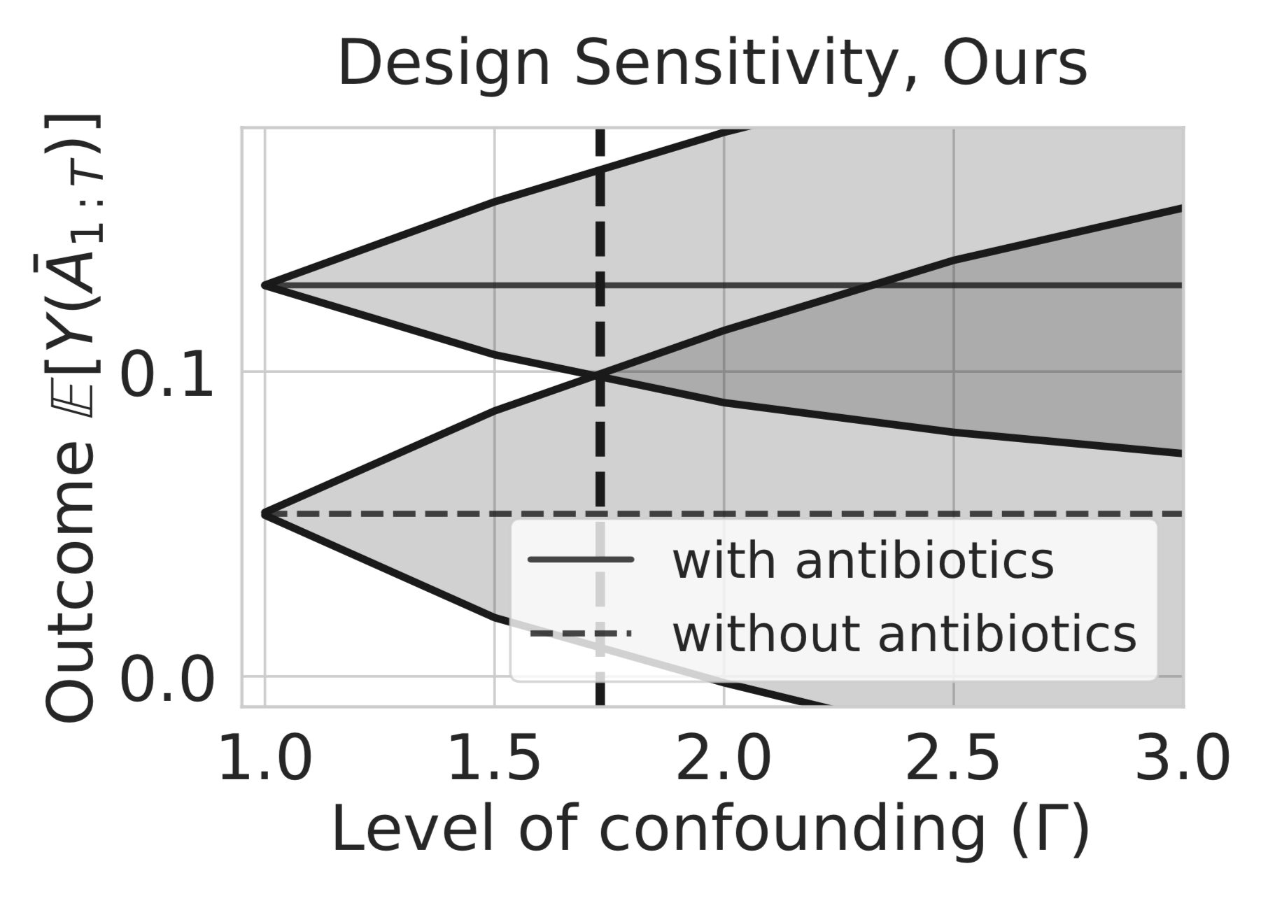
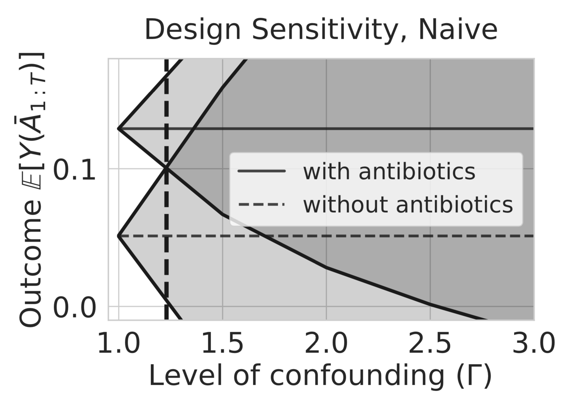
(a) Our approach	(b) Naive approach

Figure 5: Sepsis simulator design sensitivity. Data generation process with level of confounding $\Gamma^{\star}=1.0$. Estimated lower and upper bound of two policies (with and without antibiotics) under (a) our approach with sensitivity $1.7$ (b) naive approach with sensitivity $1.23$.

D.1 Sepsis Sim

We use the sepsis simulator developed by Oberst and Sontag [2019].

The optimal policy

Recall that we assume that the decisions are made near-optimally. To learn the optimal policy, we generate 2000 samples for each transition and constructed the transition matrix $P(s,a,s^{\prime})$ and the reward matrix $R(s,a,s^{\prime})$ of the MDP. Similar to Oberst and Sontag [2019] we used policy iteration to learn the optimal policy. We create a near-optimal (soft optimal) policy by having the policy take a random action with probability $0.05$, and the optimal action with probability $0.95$. The value function (for the optimal policy) was computed using value iteration. The horizon is $T=5$ and the discount factor $\gamma=0.99$, which results in soft optimal policy having an average value (over the possible distribution of state states) of $0.14$.

Confounding

We injected confounding in the first decision of this simulation by defining two different policies: “with antibiotics” and “without antibiotics”. “with antibiotics” which is identical to the soft optimal policy except that the probability mass of actions without antibiotics is moved to the corresponding action with antibiotics. For example, if the probability of the action $a_{1}=$(antibiotics on, vasopressors off, ventilation on) in the soft optimal policy is $p_{1}$, and $a_{1}^{\prime}=$(antibiotics off, vasopressors off, ventilation on) is $p_{1}^{\prime}$, then in the “with antibiotics” $a_{1}$ has probability $p_{1}+p_{1}^{\prime}$ and $a_{1}^{\prime}$ has probability zero in this new policy. The “without antibiotics” does the opposite: moves probability mass of actions with antibiotics to the corresponding action without antibiotics. In our confounding scenario, for healthy patients we administer antibiotics (i.e. follow the “with antibiotics”) policy with a higher probability (w.p. $\frac{\sqrt{\Gamma}}{1+\sqrt{\Gamma}}$). For unhealthy patients, we administer antibiotics with a lower probability (w.p. $\frac{1}{1+\sqrt{\Gamma}}$).

Concretely, to compute the transition from a state conditional on an action, we do inverse transform sampling: we generate a uniform random variable $U_{t}$ on $[0,1]$, and use this to index into the transition probability distribution for the next state, sorted by the states’ value function and current reward. This coupling ensures that if $U_{t}$ is large, then the next state will have a high value, and if $U_{t}$ is small, then the next state will have a low value. The hidden variable $U$ used for confounding in the first decision is $U=\sum_{t=1}^{T}U_{t}$, which serves as a surrogate for the health of patient, because the larger $U$ is, the more likely the patient is to have improving state values. We choose a threshold $u_{0}$, and if $U>u_{0}$, the behavior policy follows the action with antibiotics, and if $U\leq u_{0}$, the behavior policy follows the action without antibiotics, thus introducing confounding.

After the first decision, the behaviour policy is a mixture of two policies: $85\%$ the soft optimal policy and $15\%$ of a sub-optimal policy that is similar to the soft optimal but the vasopressors action is flipped. For example, if probability of the action $a_{1}=$(antibiotics on, vasopressors off, ventilation on) is $p_{1}$, and $a_{1}^{\prime}=$(antibiotics on, vasopressors on, ventilation on) in $p_{1}^{\prime}$ in the soft optimal policy, then the sub-optimal has probability $p_{1}^{\prime}$ and $p_{1}$ for action $a_{1}$ and $a_{1}^{\prime}$, respectively.

Loss minimization

Since the state and action space are discrete, we learn the tabular value $\kappa(s,a)$ for each state action pair separately to minimize the empirical loss. Additionally, in order to compute the upper bound of both ours and the naive method, we compute the negative of the lower bound on the negative of return (cost).

Behaviour Policy

We estimate the behaviour policies from the data in two parts: the first time step and time steps $t=2$ through $t=5$. By the assumptions stated above, each of these policies depends only on the previous state, and we learn the tabular probability of each state action pair $\pi_{t}(a|s)$ separately.

Design Sensitivity

We present another design sensitivity experiment, with $\Gamma^{{}^{\star}}=1.0$. Figure 5 (a,b) shows design sensitivity of our method ($1.7$) versus the naïve method ($1.23$).

D.2 Autism

In the autism experiments, our data generation process (simulator) is adopted from Lu et al. [2016, Appendix B]. Each individual has a set of covariates $X$, consisting of six mean-centered features: {age, gender, indicator of African American, indicator of Caucasian, indicator of Hispanic, indicator of Asian}. The Autism SMART trial [Kasari et al., 2014] simulator specifies a set of 300 individuals: to obtain a sample size $N$, we sample with replacement from this set. For details on the simulator, we refer to Appendix B of Lu et al. [2016]. At the first timestep there are two actions available $A_{1}\in\{-1,1\}$, where $A_{1}=1$ denote BLI, and $A_{1}=-1$ denote AAC. At the second timestep there are three actions $A_{2}\in\{-1,0,1\}$, where $A_{2}=1$ denote assigning intensified BLI to slow responders, $A_{2}=-1$ denote assigning AAC to slow responder and $A_{2}=0$ denote continuing with the same action for fast responders.

Confounding

The original simulator did not have confounding. We now describe how we introduce confounding in this setting.

Lu et al. [2016, Appendix B] specifies the effect of the second action (whether to augment BLI with AAC) on the reward outcome $Y$ as follows:

$$Y=\eta^{T}_{31}X+\eta_{22}Y_{0}+\eta_{33}^{T}A_{1}+\eta_{34}Y_{12}-2\theta(1-R)(A_{1}+1)A_{2}+\epsilon.$$

$A_{1}$ is either $-1$ or $1$. Therefore the final term (outside of the noise $\epsilon$) is non-zero only when $A_{1}=1$, and we can interpret $\theta$ as the effect size of the adaptive policy (which always takes $A_{1}=1$); for exact definition of the effect size refer to Lu et al. [2016]. For those more familiar with the RL literature, it is related to the advantage function. In the original paper, Figure 7 in Lu et al. [2016] were generated using 4 different values of $\theta$.

We introduce confounding by varying $\theta$ (thereby impacting the potential outcome) and then altering the behavioral treatment decisions according to the knowledge of that $\theta$. More precisely, given a $\theta_{0}$, for each individual, we randomly set $\theta_{0}+\sigma_{\theta}$ or $\theta_{0}-\sigma_{\theta}$. The second action is 1 with probability $\frac{\sqrt{\Gamma}}{1+\sqrt{\Gamma}}$ if $\theta\geq\theta_{0}$ and 1 with probability $\frac{1}{1+\sqrt{\Gamma}}$ if $\theta\leq\theta_{0}$. In our experiments, we take $\sigma_{\theta}=5$.

Loss minimization

To estimate $\kappa(H_{t^{\star}};a_{t^{\star}})$ in the loss minimization problem, we used a neural network with 3 hidden layers of size {128, 128, 128, 64} with Relu activations, followed by a single linear output layer. We initialize the layers with Xavier initialization and used the Adam optimizer with learning rate $10^{-3}$. The input $H_{t}$ is 10-dimensional consisting of 6 covariates, indicator of slow responder, initial action $A_{1}$, number of speech utterances after the initial action, and an interaction term between $A_{1}$ and the slow responder indicator.

Behaviour Policy

We use logistic regression to estimate the behaviour policy from the observed data: note that this is not the true behavior policy, because that depends on the (latent) confounding. Different models were fit for the first and second time steps. For the first timestep the learned model is $\pi_{1}(A_{1}|H_{1})$, where $H_{1}$ contains the observed $X$ (6 covariates), and $A_{1}\in\{-1,1\}$. For the estimated behavior policy in the second timestep $\pi_{2}(A_{2}|H_{2})$, $H_{2}$ includes $X$ (6 covariates), the action $A_{1}$, indicator of slow responder, the interaction term between $A_{1}$ and the indicator, and the number of speech utterances after the initial action.

References

- Agarwal et al. (2016) A. Agarwal, S. Bird, M. Cozowicz, L. Hoang, J. Langford, S. Lee, J. Li, D. Melamed, G. Oshri, O. Ribas, et al. Making contextual decisions with low technical debt. arXiv:1606.03966, 2016.
- Anderson et al. (2009) D. K. Anderson, R. S. Oti, C. Lord, and K. Welch. Patterns of growth in adaptive social abilities among children with autism spectrum disorders. Journal of Abnormal Child Psychology, 37(7):1019–1034, Oct 2009. ISSN 1573-2835. doi: 10.1007/s10802-009-9326-0. URL https://doi.org/10.1007/s10802-009-9326-0.
- Åstebro and Elhedhli (2006) T. Åstebro and S. Elhedhli. The effectiveness of simple decision heuristics: Forecasting commercial success for early-stage ventures. Management Science, 52(3):395–409, 2006.
- Brent (2017) A. J. Brent. Meta-analysis of time to antimicrobial therapy in sepsis: Confounding as well as bias. Critical Care Medicine, 45(2), 2017.
- Brumback et al. (2004) B. A. Brumback, M. A. Hernán, S. J. P. A. Haneuse, and J. M. Robins. Sensitivity analyses for unmeasured confounding assuming a marginal structural model for repeated measures. Statistics in Medicine, 23(5):749–767, 2004.
- Cornfield et al. (1959) J. Cornfield, W. Haenszel, E. C. Hammond, A. M. Lilienfeld, M. B. Shimkin, and E. L. Wynder. Smoking and lung cancer: Recent evidence and a discussion of some questions. Journal of the National Cancer Institute, 22(1):173–203, 1959.
- Danziger et al. (2011) S. Danziger, J. Levav, and L. Avnaim-Pesso. Extraneous factors in judicial decisions. Proceedings of the National Academy of Sciences, 108(17):6889–6892, 2011.
- Dhami (2003) M. K. Dhami. Psychological models of professional decision making. Psychological Science, 14(2):175–180, 2003.
- Fujimoto et al. (2019) S. Fujimoto, D. Meger, and D. Precup. Off-policy deep reinforcement learning without exploration. In Proceedings of the 36th International Conference on Machine Learning, 2019.
- Futoma et al. (2018) J. Futoma, A. Lin, M. Sendak, A. Bedoya, M. Clement, C. O’Brien, and K. Heller. Learning to treat sepsis with multi-output gaussian process deep recurrent q-networks, 2018. URL https://openreview.net/forum?id=SyxCqGbRZ.
- Gottesman et al. (2019a) O. Gottesman, F. Johansson, M. Komorowski, A. Faisal, D. Sontag, F. Doshi-Velez, and L. A. Celi. Guidelines for reinforcement learning in healthcare. Nature Medicine, 25(1):16–18, 2019a.
- Gottesman et al. (2019b) O. Gottesman, F. Johansson, M. Komorowski, A. Faisal, D. Sontag, F. Doshi-Velez, and L. A. Celi. Guidelines for reinforcement learning in healthcare. Nat Med, 25(1):16–18, 2019b.
- Gottesman et al. (2019c) O. Gottesman, Y. Liu, S. Sussex, E. Brunskill, and F. Doshi-Velez. Combining parametric and nonparametric models for off-policy evaluation. In International Conference on Machine Learning, pages 2366–2375, 2019c.
- Hallak and Mannor (2017) A. Hallak and S. Mannor. Consistent on-line off-policy evaluation. In Proceedings of the 34th International Conference on Machine Learning-Volume 70, pages 1372–1383. JMLR. org, 2017.
- Hanna et al. (2019) J. Hanna, S. Niekum, and P. Stone. Importance sampling policy evaluation with an estimated behavior policy. In Proceedings of the 36th International Conference on Machine Learning (ICML), June 2019.
- Hanna et al. (2017) J. P. Hanna, P. Stone, and S. Niekum. Bootstrapping with models: Confidence intervals for off-policy evaluation. In Thirty-First AAAI Conference on Artificial Intelligence, 2017.
- Hernán and Robins (2020) M. Hernán and J. Robins. Causal Inference: What If. Boca Raton: Chapman & Hall/CRC, 2020.
- Howell and Davis (2017) M. D. Howell and A. M. Davis. Management of Sepsis and Septic Shock. JAMA, 317(8):847–848, 02 2017. ISSN 0098-7484. doi: 10.1001/jama.2017.0131. URL https://doi.org/10.1001/jama.2017.0131.
- Hu et al. (1989) T.-C. Hu, F. Moricz, and R. Taylor. Strong laws of large numbers for arrays of rowwise independent random variables. Acta Mathematica Hungarica, 54(1-2):153–162, 1989.
- Imbens (2003) G. W. Imbens. Sensitivity to exogeneity assumptions in program evaluation. American Economic Review, 93(2):126–132, 2003.
- Jiang and Li (2015) N. Jiang and L. Li. Doubly robust off-policy value evaluation for reinforcement learning. arXiv preprint arXiv:1511.03722, 2015.
- Johnson et al. (2016) A. E. Johnson, T. J. Pollard, L. Shen, H. L. Li-wei, M. Feng, M. Ghassemi, B. Moody, P. Szolovits, L. A. Celi, and R. G. Mark. Mimic-iii, a freely accessible critical care database. Scientific data, 3:160035, 2016.
- Jung et al. (2018) J. Jung, R. Shroff, A. Feller, and S. Goel. Algorithmic decision making in the presence of unmeasured confounding. arXiv:1805.01868 [stat.ME], 2018.
- Kallus and Uehara (2019) N. Kallus and M. Uehara. Double reinforcement learning for efficient off-policy evaluation in markov decision processes. arXiv preprint arXiv:1908.08526, 2019.
- Kallus and Zhou (2018) N. Kallus and A. Zhou. Confounding-robust policy improvement. In Advances in Neural Information Processing Systems, pages 9269–9279, 2018.
- Kallus et al. (2018) N. Kallus, X. Mao, and A. Zhou. Interval estimation of individual-level causal effects under unobserved confounding. arXiv preprint arXiv:1810.02894, 2018.
- Kasari et al. (2014) C. Kasari, A. Kaiser, K. Goods, J. Nietfeld, P. Mathy, R. Landa, S. Murphy, and D. Almirall. Communication interventions for minimally verbal children with autism: A sequential multiple assignment randomized trial. Journal of the American Academy of Child & Adolescent Psychiatry, 53(6):635–646, 2014.
- King and Wets (1991) A. J. King and R. J. Wets. Epi-consistency of convex stochastic programs. Stochastics and Stochastic Reports, 34(1-2):83–92, 1991.
- Komorowski et al. (2018a) M. Komorowski, L. A. Celi, O. Badawi, A. C. Gordon, and A. A. Faisal. The artificial intelligence clinician learns optimal treatment strategies for sepsis in intensive care. Nature Medicine, 24(11):1716–1720, 2018a.
- Komorowski et al. (2018b) M. Komorowski, L. A. Celi, O. Badawi, A. C. Gordon, and A. A. Faisal. The artificial intelligence clinician learns optimal treatment strategies for sepsis in intensive care. Nature medicine, 24(11):1716–1720, 2018b.
- Kumar et al. (2019) A. Kumar, J. Fu, M. Soh, G. Tucker, and S. Levine. Stabilizing off-policy q-learning via bootstrapping error reduction. In Advances in Neural Information Processing Systems, pages 11761–11771, 2019.
- Le et al. (2019) H. M. Le, C. Voloshin, and Y. Yue. Batch policy learning under constraints. arXiv preprint arXiv:1903.08738, 2019.
- Liu et al. (2018a) Q. Liu, L. Li, Z. Tang, and D. Zhou. Breaking the curse of horizon: Infinite-horizon off-policy estimation. In Advances in Neural Information Processing Systems 31, pages 5356–5366, 2018a.
- Liu et al. (2018b) Y. Liu, O. Gottesman, A. Raghu, M. Komorowski, A. A. Faisal, F. Doshi-Velez, and E. Brunskill. Representation balancing mdps for off-policy policy evaluation. In Advances in Neural Information Processing Systems, pages 2644–2653, 2018b.
- Liu et al. (2019) Y. Liu, A. Swaminathan, A. Agarwal, and E. Brunskill. Off-policy policy gradient with state distribution correction. In Proceedings of the 35th Conference on Uncertainty in Artificial Intelligence, 2019.
- Lu et al. (2016) X. Lu, I. Nahum-Shani, C. Kasari, K. G. Lynch, D. W. Oslin, W. E. Pelham, G. Fabiano, and D. Almirall. Comparing dynamic treatment regimes using repeated-measures outcomes: modeling considerations in smart studies. Statistics in medicine, 35(10):1595–1615, 2016.
- Luenberger (1969) D. Luenberger. Optimization by Vector Space Methods. Wiley, 1969.
- Manski (1990) C. F. Manski. Nonparametric bounds on treatment effects. The American Economic Review, 80(2):319–323, 1990.
- McDonald (1996) C. J. McDonald. Medical heuristics: the silent adjudicators of clinical practice. Annals of Internal Medicine, 124(1_Part_1):56–62, 1996.
- Murphy (2003) S. A. Murphy. Optimal dynamic treatment regimes. Journal of the Royal Statistical Society: Series B (Statistical Methodology), 65(2):331–355, 2003.
- Murphy et al. (2001) S. A. Murphy, M. J. van der Laan, and J. M. Robins. Marginal mean models for dynamic regimes. Journal of the American Statistical Association, 96(456):1410–1423, 2001.
- Nie et al. (2019) X. Nie, E. Brunskill, and S. Wager. Learning when-to-treat policies. arXiv preprint arXiv:1905.09751, 2019.
- Oberst and Sontag (2019) M. Oberst and D. Sontag. Counterfactual off-policy evaluation with Gumbel-max structural causal models. In K. Chaudhuri and R. Salakhutdinov, editors, Proceedings of the 36th International Conference on Machine Learning, volume 97 of Proceedings of Machine Learning Research, pages 4881–4890, Long Beach, California, USA, 09–15 Jun 2019. PMLR. URL http://proceedings.mlr.press/v97/oberst19a.html.
- Pearl (2009) J. Pearl. Causality. Cambridge University Press, 2009.
- Raghu et al. (2017) A. Raghu, M. Komorowski, L. A. Celi, P. Szolovits, and M. Ghassemi. Continuous state-space models for optimal sepsis treatment-a deep reinforcement learning approach. arXiv preprint arXiv:1705.08422, 2017.
- Rhodes et al. (2017) A. Rhodes, L. E. Evans, W. Alhazzani, et al. Surviving sepsis campaign: International guidelines for management of sepsis and septic shock: 2016. Intensive Care Medicine, 43(3):304–377, 2017.
- Robins (1986) J. Robins. A new approach to causal inference in mortality studies with a sustained exposure period—application to control of the healthy worker survivor effect. Mathematical modelling, 7(9-12):1393–1512, 1986.
- Robins (1997) J. M. Robins. Causal inference from complex longitudinal data. In Latent variable modeling and applications to causality, pages 69–117. Springer, 1997.
- Robins (2004) J. M. Robins. Optimal structural nested models for optimal sequential decisions. In Proceedings of the Second Seattle Symposium in Biostatistics, pages 189–326. Springer, 2004.
- Robins et al. (2000) J. M. Robins, A. Rotnitzky, and D. O. Scharfstein. Sensitivity analysis for selection bias and unmeasured confounding in missing data and causal inference models. In M. E. Halloran and D. Berry, editors, Statistical Models in Epidemiology, the Environment, and Clinical Trials, pages 1–94, New York, NY, 2000. Springer New York. ISBN 978-1-4612-1284-3.
- Rockafellar and Wets (1998) R. T. Rockafellar and R. J. B. Wets. Variational Analysis. Springer, New York, 1998.
- Rosenbaum (2002) P. R. Rosenbaum. Observational studies. In Observational studies, pages 1–17. Springer, 2002.
- Rosenbaum (2010) P. R. Rosenbaum. Design of Observational Studies, volume 10. Springer, 2010.
- Rosenbaum and Rubin (1983) P. R. Rosenbaum and D. B. Rubin. Assessing sensitivity to an unobserved binary covariate in an observational study with binary outcome. Journal of the Royal Statistical Society: Series B (Methodological), 45(2):212–218, 1983.
- Rutter et al. (1967) M. Rutter, D. Greenfeld, and L. Lockyer. A five to fifteen year follow-up study of infantile psychosis: Ii. social and behavioural outcome. British Journal of Psychiatry, 113(504):1183–1199, 1967. doi: 10.1192/bjp.113.504.1183.
- Seymour et al. (2017) C. W. Seymour, F. Gesten, H. C. Prescott, M. E. Friedrich, T. J. Iwashyna, G. S. Phillips, S. Lemeshow, T. Osborn, K. M. Terry, and M. M. Levy. Time to treatment and mortality during mandated emergency care for sepsis. New England Journal of Medicine, 376(23):2235–2244, 2017. doi: 10.1056/NEJMoa1703058. URL https://doi.org/10.1056/NEJMoa1703058. PMID: 28528569.
- Sterling et al. (2015) S. A. Sterling, W. R. Miller, J. Pryor, M. A. Puskarich, and A. E. Jones. The impact of timing of antibiotics on outcomes in severe sepsis and septic shock: a systematic review and meta-analysis. Critical care medicine, 43(9):1907, 2015.
- Thomas and Brunskill (2016) P. Thomas and E. Brunskill. Data-efficient off-policy policy evaluation for reinforcement learning. In International Conference on Machine Learning, pages 2139–2148, 2016.
- Thomas et al. (2015) P. S. Thomas, G. Theocharous, and M. Ghavamzadeh. High-confidence off-policy evaluation. In Twenty-Ninth AAAI Conference on Artificial Intelligence, 2015.
- Thomas et al. (2019) P. S. Thomas, B. C. da Silva, A. G. Barto, S. Giguere, Y. Brun, and E. Brunskill. Preventing undesirable behavior of intelligent machines. Science, 366(6468):999–1004, 2019.
- Wübben and Wangenheim (2008) M. Wübben and F. v. Wangenheim. Instant customer base analysis: Managerial heuristics often “get it right”. Journal of Marketing, 72(3):82–93, 2008.
- Xie et al. (2019) T. Xie, Y. Ma, and Y.-X. Wang. Towards optimal off-policy evaluation for reinforcement learning with marginalized importance sampling. In Advances in Neural Information Processing Systems 32, pages 9665–9675, 2019.
- Yadlowsky et al. (2018) S. Yadlowsky, H. Namkoong, S. Basu, J. Duchi, and L. Tian. Bounds on the conditional and average treatment effect in the presence of unobserved confounders. arXiv:1808.09521 [stat.ME], 2018.
- Zhang and Bareinboim (2019) J. Zhang and E. Bareinboim. Near-optimal reinforcement learning in dynamic treatment regimes. In Advances in Neural Information Processing Systems 32, pages 13401–13411, 2019.