Geometrical Formulation of Adiabatic Pumping as a Heat Engine

Abstract

We investigate a heat engine under an adiabatic (Thouless) pumping process. In this process, the extracted work and lower bound on dissipated availability are characterized by a vector potential and a Riemannian metric tensor, respectively. We derive a trade-off relation between the power and effective efficiency. We also explicitly calculate the trade-off relation as well as the power and effective efficiency for a spin-boson model coupled to two reservoirs.

I INTRODUCTION

An average current can be generated even in the absence of an average bias under slow and periodic modulation of multiple parameters of the system. This is known as an adibatic pumping process. Thouless first proposed the theory of the adiabatic pumping for an isolated quantum system thouless1 ; thouless2 . He showed that electrons can be transported by applying a time-periodic potential to one-dimensional isolated quantum systems under a periodic boundary condition. He also clarified that the charge transport in this system is essentially induced by a Berry-phase-like quantity in the space of the modulation parameters thouless1 ; thouless2 ; berry ; xiao . This phenomenon has been observed experimentally in various processes such as charge transport ex-ch1 ; ex-ch2 ; ex-ch2.5 ; ex-ch3 ; ex-ch4 ; ex-ch5 ; ex-thou1 ; ex-thou2 and a spin pumping process ex-spin1 . Later, Brouwer extended the Thouless pumping to that in an open quantum system brouwer . It has been recognized that the essence of Thouless pumping can be described by a classical master equation in which the Berry-Sinitsyn-Nemenman (BSN) phase is the generator of the pumping current sinitsyn1 ; sinitsyn2 . There are various papers on geometrical pumping processes in terms of the scattering theory s-th1 ; s-th2 ; s-th3 ; s-th-ch1 ; s-th-ch2 ; s-th-ch3 ; s-th-spin1 , classical master equationsparrondo ; usmani ; astumian1 ; astumian2 ; rahav ; chernyak1 ; chernyak2 ; ren ; sagawa and quantum master equations qme1 ; qme2 ; qme-spin1 ; qme-spin2 ; yuge1 ; yuge2 . The extended fluctuation theorem for adiabatic pumping processes has also been studied watanabe ; Hino-Hayakawa ; Takahashi20JSP .

The geometrical concept is also used in finite time thermodynamics finite , in which the thermodynamic length plays a key role. The thermodynamic length is originally introduced for macroscopic systems Weinhold ; Ruppeiner ; Salamon ; Schlogl ; geo-rev , and it has been used in wide classes of thermodynamic systems such as a classical nanoscale system Crooks , a closed quantum system Deffner and an open quantum system Scandi .

Recently, Brandner and Saito have formulated the geometrical thermodynamics for a microscopic heat engine in the adiabatic regime Brandner-Saito . In their approach, the properties of the working system are discribed by a vector potential and a Riemannian metric tensor in the space of control parameters. If one chooses a driving protocol, an effective flux and a length are assigned to the protocol. Then, they provide the extracted work and lower bound of the dissipated availability. On the other hand, Giri and Goswami proposed a quantum heat engine which includes the effect of the BSN phase by controlling temperatures of reservoirs engine .

Nevertheless, we cannot apply the previous formulations to a heat engine undergoing an adiabatic pumping process with equal average temperature in both reservoirs, because (i) Ref. Brandner-Saito only considered systems coupled to a single reservoir near an equilibrium state and (ii) Ref. engine only considered the situation where the temperature of one of the reservoirs is always higher than that of the other one. Note that the outcome in the latter case is dominated by the dynamical phase. Namely, it is difficult to observe the geometrical contribution in such a system. In this paper, therefore, we extend the geometrical formulations of Refs. Brandner-Saito and engine to a system which is coupled to two reservoirs with equal average temperature under adiabatic modulation of thermodynamic quantities of the reservoirs and the target system. In the adiabatic regime, we obtain a geometrical representation of the extracted work and a lower bound of dissipated availability. We also derive a trade-off relation between the power and effective efficiency.

The organization of this paper is as follows. In Sec. II, we explain the setup and geometrical formulation for describing the heat engine under an adiabatic pumping process. In Sec. III, we apply our formulation to a two-level spin-boson system coupled to two reservoirs. Finally, we discuss and summarize our results in Sec. IV. In Appendix A, we present a mathematical description of the pseudo-inverse of transition matrix. In Appendix B, we explain the outline of the perturbation theory of the master equation with slowly modulated parameters. In Appendix C, we summarize the detailed setup of the spin-boson model used in the main text.

II GENERAL FRAMEWORK

II.1 Setup

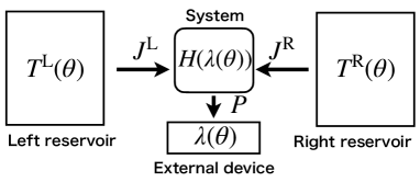
Figure 1: A schematic of the total system which consists of the target system and the left and right reservoirs. We periodically control the temperatures of the reservoirs $T^{\mathrm{L}}$, $T^{\mathrm{R}}$ and the parameter $\lambda$ of the system Hamiltonian $\hat{H}(\lambda)$ by the external device. $J^{\mathrm{L}}$ and $J^{\mathrm{R}}$ are the heat currents from the left and right reservoirs to the system, respectively. $P$ is the averaged power extracted from the system.

In this paper, we consider a system S coupled to two reservoirs L and R under periodic modulation of parameters with the period $\tau_{\mathrm{p}}$. A schematic of our system is depicted in Fig. 1. Each reservoir $\alpha=$L or R is characterized by the temperature $T^{\alpha}$. We assume that the system S is characterized by $n$ discrete states $i=0,\dots,n-1$. The system Hamiltonian $\hat{H}(\lambda)$ is characterized by its eigenvalue $E_{i}(\lambda)$ of $i-$th state with a control parameter $\lambda$. In this paper, we control the set of parameters $\bm{\Lambda}:=(\lambda,T^{\mathrm{L}},T^{\mathrm{R}})$.

We assume that the dynamics of S is described by a master equation

$$\frac{d}{d\theta}|p(\theta)\rangle=\epsilon^{-1}\hat{K}(\bm{\Lambda}(\theta))|p(\theta)\rangle.$$ (1)

Here we have introduced the dimensionless time (which is the phase in the modulation) $\theta:=(t-t_{0})/\tau_{\mathrm{p}}$ and the dimensionless operation speed $\epsilon:=1/(\tau_{\mathrm{p}}\Gamma)$, where $t_{0}$ is the time after which the system reaches a periodic state and $\Gamma$ is the coupling strength or the characteristic transition rate between the system and the reservoirs. The explicit expression of $\Gamma$ for the spin-boson model is presented in Appendix C. We have also introduced the vector $|p(\theta)\rangle:=(p_{0}(\theta),\dots,p_{n-1}(\theta))^{T}$, where $p_{i}(\theta)$ is the probability of state $i$ at $\theta$. The vector $|p(\theta)\rangle$ satisfies $0\leq p_{i}(\theta)\leq 1$ and $\langle 1|p(\theta)\rangle=\sum_{i}p_{i}(\theta)=1$, where $\langle 1|:=(1,\dots,1)$. The matrix $\hat{K}(\bm{\Lambda}(\theta))=\sum_{\alpha=\mathrm{L},\mathrm{R}}\hat{K}^{\alpha}(\bm{\Lambda}(\theta)):=\sum_{\alpha=\mathrm{L},\mathrm{R}}(k^{\alpha}_{ij}(\bm{\Lambda}(\theta)))$ is the transition matrix and its ($ij$)-component $k^{\alpha}_{ij}(\bm{\Lambda}(\theta))$ is the transition rate of $j\to i$ due to interaction with the reservoir $\alpha$ at $\theta$. $\hat{K}(\bm{\Lambda}(\theta))$ satisfies $\langle 1|\hat{K}(\bm{\Lambda}(\theta))=0$. We assume that the $\theta$-dependence of $\hat{K}(\bm{\Lambda}(\theta))$ only appears through the control parameters $\bm{\Lambda}(\theta)$. We also assume that $\hat{K}^{\alpha}(\bm{\Lambda}(\theta))$ satisfies the detailed balance relation

$$\ln\frac{k^{\alpha}_{ij}(\bm{\Lambda}(\theta))}{k^{\alpha}_{ji}(\bm{\Lambda}(\theta))}=-\beta^{\alpha}(\theta)\left[E_{i}(\lambda(\theta))-E_{j}(\lambda(\theta))\right],$$ (2)

where $\beta^{\alpha}({\theta}):=1/T^{\alpha}({\theta})$ is the inverse temperature of the reservoir $\alpha$ at $\theta$. We assume that the master equation (1) has a unique steady state $|p^{\mathrm{ss}}(\bm{\Lambda}(\theta))\rangle$ which satisfies $\hat{K}(\bm{\Lambda}(\theta))|p^{\mathrm{ss}}(\bm{\Lambda}(\theta))\rangle=0$. Since the system is coupled to two reservoirs having different temperatures, $|p^{\mathrm{ss}}(\bm{\Lambda}(\theta))\rangle$ is a nonequilibrium steady state.

II.2 Thermodynamic Quantities

The performance of a heat engine is governed by the second law of thermodynamics, i. e. the non-negativity of the total entropy production rate. When the system is coupled to a single heat reservoir, the second law of thermodynamics is achieved by a quasi-static operation. On the other hand, when the system is coupled to multiple heat reservoirs, a proper nonequilibrium entropy production should be non-negative for arbitrary operations. Such a non-negative quantity is known as the Hatano-Sasa (HS) entropy production rate $\sigma^{\rm HS}(\theta)$ Hatano-Sasa defined as

$$\sigma^{\mathrm{HS}}(\theta):=\dot{S}(\theta)+\sigma^{\mathrm{ex}}(\theta),$$ (3)

where

$$S(\theta):=\langle 1|\hat{s}(\theta)|p(\theta)\rangle$$ (4)

with its element $s_{ij}(\theta)$ of $\hat{s}(\theta)$

$$s_{ij}(\theta):=-\ln p_{i}(\theta)\delta_{ij}$$ (5)

is the Shannon entropy of the system S with the notation $\dot{S}(\theta):=dS(\theta)/d\theta$. Equation (3) contains the excess entropy production rate $\sigma^{\mathrm{ex}}(\theta)$ defined as

$$\sigma^{\mathrm{ex}}(\theta):=-\langle 1|\hat{\phi}(\bm{\Lambda}(\theta))|\dot{p}(\theta)\rangle,$$ (6)

where the element $\phi_{ij}(\bm{\Lambda}(\theta))$ of $\hat{\phi}(\bm{\Lambda}(\theta))$ satisfies

$${\phi}_{ij}(\bm{\Lambda}(\theta)):=-\ln p^{\mathrm{ss}}_{i}(\bm{\Lambda}(\theta))\delta_{ij}.$$ (7)

It is known that HS entropy production rate $\sigma^{\rm HS}$ is always non-negative and converges to zero in quasi-static limit $\epsilon\to 0$, thanks to the HS inequality Hatano-Sasa .

To discuss the performance of the heat engine, we introduce the dissipative availability Salamon ; Brandner-Saito defined as

$$A:=\int^{1}_{0}T(\theta)\sigma^{\mathrm{HS}}(\theta)d\theta,$$ (8)

where $T(\theta):=\beta(\theta)^{-1}$ with $\beta(\theta):=[\beta^{\mathrm{L}}(\theta)+\beta^{\mathrm{R}}(\theta)]/2$. According to HS inequality $\sigma^{\mathrm{HS}}(\theta)\geq 0$ the dissipative availability is always non-negative, i. e. $A\geq 0$. Thus, $A$ plays a key role in nonequilibrium thermodynamics. $A$ can be decomposed as

$$A=U+V-W,$$ (9)

where

$$W:=-\int^{1}_{0}\left\langle 1\left|\frac{\partial\hat{H}(\lambda(\theta))}{\partial\lambda(\theta)}\right|p(\theta)\right\rangle\dot{\lambda}(\theta)d\theta$$ (10)

is the work extracted from the system per cycle. Here, $U$ defined as

$$U:=-\int^{1}_{0}S(\theta)\dot{T}(\theta)d\theta$$ (11)

is the thermal energy which can be used even in nonequilibrium processes Brandner-Saito , while $V$ defined as

$$V:=\int^{1}_{0}\left\langle 1\left|\frac{\partial\hat{X}(\bm{\Lambda}(\theta))}{\partial\Lambda^{\mu}(\theta)}\right|p(\theta)\right\rangle\dot{\Lambda}^{\mu}(\theta)d\theta$$ (12)

is a nonequilibrium potential which exists only if the system is coupled to multiple reservoirs. Here we have introduced a matrix $\hat{X}(\bm{\Lambda}(\theta)):=T(\theta)[\hat{\phi}(\bm{\Lambda}(\theta))-\hat{H}(\lambda(\theta))]$ and $\Delta(\theta):=[\beta^{\mathrm{L}}(\theta)-\beta^{\mathrm{R}}(\theta)]/2$. Since $\bm{\Lambda}=(\lambda,T^{\mathrm{L}},T^{\mathrm{R}})$ can be converted into $\bm{\Lambda}=(\lambda,T,\Delta)$, we use the notation $\Lambda^{\mu}$ to express one of $(\lambda,T,\Delta)$, i.e. $\Lambda^{0}=\lambda$, $\Lambda^{1}=T$ and $\Lambda^{2}=\Delta$ for later discussion. We also use Einstein’s summation convention for $\mu=0,1,2$ in this paper. Since $A\geq 0$, the extracted work $W$ is bounded as

$$W=U+V-A\leq U+V.$$ (13)

Thus, we can interpret $U+V$ as the available energy which can be converted into the work. If a system is coupled to only one reservoir, the dissipative availability $A$ is reduced to $A=U-W$ Brandner-Saito , which is equivalent to $W\leq U$. Therefore, our dissipative availability $A$ is a nonequilibrium extension of the dissipative availability introduced in Refs. Salamon ; Brandner-Saito .

Let us introduce the ratio of the work $W$ to the available energy $U+V$ as

$$\xi:=\frac{W}{U+V}=\frac{W}{W+A}.$$ (14)

Because of $A\geq 0$, $\xi$ satisfies $0\leq\xi\leq 1$. Thus, we call $\xi$ the effective efficiency because it is an indicator of the performance of the heat engine. In the quasi-static limit ($\epsilon\to 0$, i. e. $A\to 0$), $\xi$ converges to $1$. The scaled power defined as

$$P:=\epsilon W$$ (15)

converges to zero in this limit. Note that $P$ does not have the dimension of power because we measure time scale by the dimensionless parameter $\epsilon$ under the fixing $\Gamma$. To obtain larger power, we need the higher speed $\epsilon$ of operation, in which the effective efficiency $\xi$ becomes smaller. In the next subsection, we discuss such a trade-off relation in the linear response regime.

We note that the conventional thermal efficiency is written as

$$\eta:=\frac{W}{Q_{\mathrm{in}}},$$ (16)

where

$$Q_{\mathrm{in}}:=\sum_{\alpha=\mathrm{L},\mathrm{R}}\int^{1}_{0}d\theta\max[J^{\alpha}(\theta),0]$$ (17)

is the heat absorbed by the system in one cycle and

$$J^{\alpha}(\theta):=\epsilon^{-1}\langle 1|\hat{H}(\lambda(\theta))\hat{K}^{\alpha}(\bm{\Lambda}(\theta))|p(\theta)\rangle$$ (18)

is the heat current from the reservoir $\alpha$ to the system S at $\theta$. If the temperature difference between two reservoirs is finite, the leading term of $J^{\alpha}(\theta)$ is $O(\epsilon^{-1})$. Thus, the thermal efficiency $\eta$ is $O(\epsilon)$, which converges to zero in the quasi-static limit.

Let us briefly summarize difference between the effective efficiency $\xi$ and conventional efficiency $\eta$. The former is the efficiency to express the conversion rate from the available source $U+V$ to the work $W$ once a nonequilibrium steady state is achieved, while the latter is the conversion rate from the absorbing heat to the work. Both efficiencies prefer zero entropy productions to get high performance, but there are several intrinsic differences. It should be noted that most of absorbing heat in a nonequilibrium engine is consumed as the housekeeping heat. Therefore, $\xi$ is much higher than $\eta$ in general. Moreover, the heat engine under Thouless pumping we consider in this paper is driven by reservoirs coupled to equal average temperature. Therefore, $\eta$ becomes zero in the limit $\epsilon\to 0$.

For later discussion, let us rewrite the dissipative availability $A$. Substituting Eqs. (3)-(7) into Eq. (8) with the integral by part $A$ can be rewritten as

$$A= \tilde{A}^{(0)}+\tilde{A}^{(1)}$$ (19)

where

$$\tilde{A}^{(0)}:=-\int^{1}_{0}\langle 1|[\hat{s}(\theta)-\hat{\phi}(\bm{\Lambda}(\theta))]|p(\theta)\rangle\dot{T}(\theta)d\theta$$ (20)

and

$$\tilde{A}^{(1)}:=-\int^{1}_{0}f^{\mu}(\theta)\dot{\Lambda}^{\mu}(\theta)d\theta$$ (21)

with

$$f^{\mu}(\theta):=\langle 1|\hat{F}^{\mu}(\bm{\Lambda}(\theta))|p(\theta)\rangle,$$ (22)

and

$$\hat{F}^{\mu}(\bm{\Lambda}(\theta)):=-T(\theta)\frac{\partial\hat{\phi}(\bm{\Lambda})}{\partial\Lambda^{\mu}}(\theta),$$ (23)

which is the effective force conjugate to $\dot{\Lambda}^{\mu}(\theta)$. To derive Eq. (19) we have used the periodicities of $|p(\theta)\rangle$ and the control parameters $\bm{\Lambda}(\theta)$ to omit the boundary term.

II.3 Linear response regime

In this subsection, we consider thermodynamics of the engine introduced in the previous subsection in the linear response regime for small $\epsilon$. Thanks to Appendix A, the solution of the master equation (1) in the linear response regime can be expanded as

$$|p(\theta)\rangle\simeq|p^{\mathrm{ss}}(\bm{\Lambda}(\theta))\rangle+\epsilon|p^{(1)}(\bm{\Lambda}(\theta))\rangle+O(\epsilon^{2}),$$ (24)

where the second term on the right hand side of Eq. (24) can be written as

$$|p^{(1)}(\bm{\Lambda}(\theta))\rangle=\hat{K}^{+}(\bm{\Lambda}(\theta))|\dot{p}^{\mathrm{ss}}(\bm{\Lambda}(\theta))\rangle.$$ (25)

Here $\hat{K}^{+}(\bm{\Lambda}(\theta))$ is the pseudo-inverse inverse of the transition matrix $\hat{K}(\bm{\Lambda}(\theta))$ (see Appendix B for its details), which is written as

$$\hat{K}^{+}(\bm{\Lambda})=\int^{\infty}_{0}dse^{s\hat{K}(\bm{\Lambda})}\Big{(}|p^{\mathrm{ss}}(\bm{\Lambda})\rangle\langle 1|-1\Big{)}.$$ (26)

Then, $f^{\mu}(\theta)$ can be written as

$$f^{\mu}(\theta)\simeq f_{\mathrm{ss}}^{\mu}(\bm{\Lambda}(\theta))+\epsilon R^{\mu\nu}(\bm{\Lambda}(\theta))\dot{\Lambda}^{\nu}(\theta)+O(\epsilon^{2}),$$ (27)

where we have introduced

$$f_{\mathrm{ss}}^{\mu}(\bm{\Lambda}(\theta)):=-\langle 1|\hat{F}^{\mu}(\bm{\Lambda}(\theta))|p^{\mathrm{ss}}(\bm{\Lambda}(\theta))\rangle.$$ (28)

The response matrix $R^{\mu\nu}(\bm{\Lambda}(\theta))$ introduced in Eq. (27) is defined as

$$R^{\mu\nu}(\bm{\Lambda}(\theta))=-\beta(\theta)\int^{\infty}_{0}ds\langle F^{\mu}(s);F^{\nu}(0)\rangle_{\bm{\Lambda}(\theta)},$$ (29)

where

$$\langle F^{\mu}(s);F^{\nu}(0)\rangle_{\bm{\Lambda}}$$

$$:=\left\langle 1\left|\hat{F}^{\mu}(\bm{\Lambda})e^{s\hat{K}^{+}(\bm{\Lambda})}\hat{F}^{\nu}(\bm{\Lambda})\right|p^{\mathrm{ss}}(\bm{\Lambda})\right\rangle$$

$${\leavevmode\nobreak\ }-\left\langle 1\left|\hat{F}^{\mu}(\bm{\Lambda})e^{s\hat{K}^{+}(\bm{\Lambda})}\right|p^{\mathrm{ss}}(\bm{\Lambda})\right\rangle\left\langle 1\left|\hat{F}^{\nu}(\bm{\Lambda})\right|p^{\mathrm{ss}}(\bm{\Lambda})\right\rangle$$ (30)

is the cannonical correlation between $\hat{F}^{\mu}(\bm{\Lambda})$ and $\hat{F}^{\nu}(\bm{\Lambda})$ in a steady state characterized by $\bm{\Lambda}$. Equation (II.3) is nothing but the Green-Kubo formula in nonequilibrium systems coupled to two reservoirs.

Since we focus only on the linear region of $\epsilon$ in this paper, we can ignore $\tilde{A}^{(0)}$ in Eq. (19), which is estimated as $O(\epsilon^{2})$. Thus, Eq. (19) is reduced to

$$A\simeq\tilde{A}^{(1)}.$$ (31)

Thus, substituting Eq. (27) into Eq. (21) the dissipative availability $A$ can be rewritten as

$$A\simeq -\int^{1}_{0}f_{\mathrm{ss}}^{\mu}(\bm{\Lambda}(\theta))\dot{\Lambda}^{\mu}(\theta)d\theta$$

$$-\epsilon\int^{1}_{0}R^{\mu\nu}(\bm{\Lambda}(\theta))\dot{\Lambda}^{\mu}(\theta)\dot{\Lambda}^{\nu}(\theta)d\theta$$ (32)

where the first term on the right hand side of Eq. (II.3) is zero because of $\langle 1|d\phi(\theta)/d\theta|p^{\rm ss}\rangle=-\sum_{i}p_{i}^{\rm ss}(d/d\theta)\ln p_{i}^{\rm ss}=0$ with the aid of $\frac{d}{d\theta}\sum_{i}p_{i}^{\rm ss}(\theta)=0$ and Eqs. (21) and (31). Thus, we obtain

$$A =\epsilon\mathcal{A}_{1}+O(\epsilon^{2}),$$ (33)

$$\mathcal{A}_{1}: =\int^{1}_{0}g^{\mu\nu}(\bm{\Lambda}(\theta))\dot{\Lambda}^{\mu}(\theta)\dot{\Lambda}^{\nu}(\theta)d\theta,$$ (34)

where

$$g^{\mu\nu}(\bm{\Lambda}(\theta)):=-\frac{1}{2}[R^{\mu\nu}(\bm{\Lambda}(\theta))+R^{\nu\mu}(\bm{\Lambda}(\theta))]$$ (35)

is the thermodynamic metric tensor, which is symmetric and positive semi-definite. Using the Cauchy-Schwartz inequality, the dissipative availability $A=\epsilon\mathcal{A}_{1}$ is bounded as

$$\mathcal{A}_{1}\geq\mathcal{L}^{2},$$ (36)

where

$$\mathcal{L}:=\oint_{\gamma}\sqrt{g^{\mu\nu}(\bm{\Lambda})d\Lambda^{\mu}d\Lambda^{\nu}}$$ (37)

is the thermodynamic length corresponding to the length along the trajectory $\gamma$ in Riemannian manifold with the metric $g^{\mu\nu}(\bm{\Lambda})$. The inequality (36) is one of the main results in this paper, which has an identical form to that coupled to one reservoir Brandner-Saito . The equality in Eq. (36) is held when $g^{\mu\nu}(\bm{\Lambda}(\theta))\dot{\Lambda}^{\mu}(\theta)\dot{\Lambda}^{\nu}(\theta)$ is a non-negative $\theta$-independent constant. This equality cannot be achieved if BSN phase is meaningful, because $g^{\mu\nu}(\bm{\Lambda}(\theta))\dot{\Lambda}^{\mu}(\theta)\dot{\Lambda}^{\nu}(\theta)$ should be a $\theta$-dependent variable once the trajectory in the parameter space makes a closed loop to generate BSN phase.

The average power can be approximated as

$$P=\epsilon\mathcal{W}+O(\epsilon^{2})$$ (38)

for small $\epsilon$, where

$$\mathcal{W}:=\oint_{\gamma}\mathcal{A}^{\mu}(\bm{\Lambda})d\Lambda^{\mu}$$ (39)

is the adiabatic work defined as the line integration of the thermodynamic vector potential

$$\mathcal{A}^{\mu}(\bm{\Lambda}):=\lambda\frac{\partial}{\partial\Lambda^{\mu}}\left\langle 1\left|\frac{\partial\hat{H}}{\partial\lambda}\right|p^{\mathrm{ss}}(\bm{\Lambda})\right\rangle$$ (40)

along the trajectory $\gamma$ of parameter control Brandner-Saito . Note that $\mathcal{A}^{\mu}(\bm{\Lambda})$ corresponds to the BSN vector in adiabatic pumping processes sinitsyn1 ; sinitsyn2 .

By using the equality (36), the effective efficiency $\xi$ (14) is written as

$$\xi =1-\epsilon\frac{\mathcal{A}_{1}}{\mathcal{W}}+O(\epsilon^{2}).$$ (41)

Using Eq. (36) the relation (41) can be rewritten as

$$1-\xi\geq\epsilon\frac{\mathcal{L}^{2}}{\mathcal{W}}=\epsilon^{2}\frac{\mathcal{L}^{2}}{P},$$ (42)

where we have used Eq. (15) for the final expression. This relation tells us that the decrement of the effective efficiency is bounded by the thermodynamic length $\mathcal{L}$ and $\mathcal{W}$ or the power $P$, which becomes smaller if $\mathcal{W}$ or $P$ is larger. If we regard $\epsilon$ as a control parameter, and thus $P$ as an independent variable from $\mathcal{W}$, one obtains the trade-off relation between the power and effective efficiency

$$P\leq\left(\frac{\mathcal{W}}{\mathcal{L}}\right)^{2}(1-\xi)$$ (43)

in the limit $\xi\to 1$ which is equivalent to $\epsilon\to 0$. This bound is identical to that for one reservoir Brandner-Saito . The maximum slope in Eq. (43) is determined by ${\mathcal{W}}/{\mathcal{L}}$, where $\mathcal{W}$ and $\mathcal{L}$ are the geometric quantities. To optimize the performance of the engine we should choose smaller under the condition $\mathcal{A}_{1}\to\mathcal{L}^{2}$.

It is obvious that $\xi$ in Eq. (41) becomes 1 and the power $P$ in Eq. (43) becomes zero in the adiabatic limit ($\epsilon\to 0$). This corresponds to the Carnot efficiency in the conventional thermodynamics. Note that the conventional efficiency $\eta$ introduced in Eq. (16) tends to zero in the quasi-static limit ($\epsilon\to 0$) even if $\xi$ reaches the maximum value 1 because we need the house keeping heat, though we do not know how $\eta$ depends on $\epsilon$ in general.

III APPLICATION to Spin-boson system

In this section, we apply the general framework developed in previous section to the spin-boson model in which a single spin is coupled to two bosonic reservoirs (see Fig. 2 for a schematic of our system). Under the Born-Markov approximation, the system follows the master equation. Moreover, if we ignore the initial relaxation process, the off-diagonal elements of the density matrix of the system is negligible. Thus, the system can be regarded as a classical one. Detailed formulation of the spin-boson system as a quantum system is given in Appendix C. In this section, we only consider the classical limit of this system.

III.1 2-level classical spin-boson model

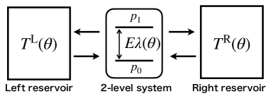
Figure 2: A schematic of a two-level spin-boson model. We periodically control the temperatures of the reservoirs $T^{\mathrm{L}}$, $T^{\mathrm{R}}$ and the parameter $\lambda$ of the system Hamiltonian $\hat{H}(\lambda)$. $E\lambda(\theta)$ is the energy difference between two states.

The system contains one spin which has two states. The system Hamiltonian is given as

$$\hat{H}(\lambda(\theta))=\left(\begin{array}[]{cc}0&0\\ 0&E\lambda(\theta)\end{array}\right),$$ (46)

where $E\lambda(\theta)$ is the energy difference between two states with the non-negative control parameter $\lambda(\theta)$. The system is coupled to two thermal reservoirs L and R characterized by temperatures $T^{\mathrm{L}}$ and $T^{\mathrm{R}}$, respectively. We control the set of parameters $\bm{\Lambda}(\theta)=(\lambda(\theta),T^{\mathrm{L}}(\theta),T^{\mathrm{R}}(\theta))$ periodically with the control speed $\epsilon$. The transition matrix $\hat{K}(\bm{\Lambda})$ of the master equation (1) is given as

$$\hat{K}(\bm{\Lambda}(\theta)) =\left(\begin{array}[]{cc}-k_{10}(\bm{\Lambda}(\theta))&k_{01}(\bm{\Lambda}(\theta))\\ k_{10}(\bm{\Lambda}(\theta))&-k_{01}(\bm{\Lambda}(\theta))\end{array}\right)$$ (49)

$$=\sum_{\alpha}\left(\begin{array}[]{cc}-n^{\alpha}(\bm{\Lambda}(\theta))&1+n^{\alpha}(\bm{\Lambda}(\theta))\\ n^{\alpha}(\bm{\Lambda}(\theta))&-1-n^{\alpha}(\bm{\Lambda}(\theta))\end{array}\right),$$ (52)

where

$$n^{\alpha}(\bm{\Lambda}(\theta))=\left(e^{\beta^{\alpha}(\theta)E\lambda(\theta)}-1\right)^{-1}$$ (53)

is the Bose distribution function in the reservoir $\alpha$ (= L, R).

The steady state of the master equation (1) is given as

$$|p^{\mathrm{ss}}(\bm{\Lambda}(\theta))\rangle =\left(\begin{array}[]{c}p^{\mathrm{ss}}_{0}(\bm{\Lambda}(\theta))\\ p^{\mathrm{ss}}_{1}(\bm{\Lambda}(\theta))\end{array}\right)$$ (56)

$$=\frac{1}{k_{01}(\bm{\Lambda}(\theta))+k_{10}(\bm{\Lambda}(\theta))}\left(\begin{array}[]{c}k_{01}(\bm{\Lambda}(\theta))\\ k_{10}(\bm{\Lambda}(\theta))\end{array}\right).$$ (59)

In $(\lambda,T,\Delta)$-representation, $|p^{\mathrm{ss}}(\bm{\Lambda})\rangle$ can be written as

$$p^{\mathrm{ss}}_{0}(\bm{\Lambda}(\theta)) =p^{\mathrm{eq}}_{0}(\lambda(\theta),\beta(\theta))$$

$${\leavevmode\nobreak\ }\left\{1+k^{\mathrm{eq}}_{10}(\lambda(\theta),\beta(\theta))\Big{[}1-\cosh{(\Delta E\lambda(\theta))}\Big{]}\right\},$$ (60)

$$p^{\mathrm{ss}}_{1}(\bm{\Lambda}) =p^{\mathrm{eq}}_{0}(\lambda(\theta),\beta(\theta))$$

$${\leavevmode\nobreak\ }\left\{1+k^{\mathrm{eq}}_{01}(\lambda(\theta),\beta(\theta))\Big{[}\cosh{(\Delta E\lambda(\theta))}-1\Big{]}\right\},$$ (61)

where

$$p^{\mathrm{eq}}_{0}(\lambda(\theta),\beta(\theta)): =\frac{1}{1+e^{-\beta(\theta)E\lambda(\theta)}},$$ (62)

$$p^{\mathrm{eq}}_{1}(\lambda(\theta),\beta(\theta)): =\frac{e^{-\beta(\theta)E\lambda(\theta)}}{1+e^{-\beta(\theta)E\lambda(\theta)}}$$ (63)

are the corresponding equilibrium states at $\beta$ for the ground state and excited state, respectively, (see Fig. 2) and

$$k^{\mathrm{eq}}_{10}(\lambda(\theta),\beta(\theta)):=\left(e^{\beta(\theta)E\lambda(\theta)}-1\right)^{-1},$$ (64)

$$k^{\mathrm{eq}}_{01}(\lambda(\theta),\beta(\theta)):=e^{\beta(\theta)E\lambda(\theta)}\left(e^{\beta(\theta)E\lambda(\theta)}-1\right)^{-1}$$ (65)

are the transition rates at $\lambda(\theta)$ and $\beta(\theta)$. Then, the diagonal elements of the matrix $\hat{X}(\bm{\Lambda}(\theta))$ in Eq. (12) are explicitly given as

$$X_{00}(\bm{\Lambda}) =-T\ln\left\{1+k^{\mathrm{eq}}_{10}(\lambda,\beta)\Big{[}1-\cosh{(\Delta E\lambda)}\Big{]}\right\},$$ (66)

$$X_{11}(\bm{\Lambda}) =-T\ln\left\{1+k^{\mathrm{eq}}_{01}(\lambda,\beta))\Big{[}\cosh{(\Delta E\lambda)}-1\Big{]}\right\},$$ (67)

where we have omitted writing $\theta$-dependence.

III.2 Numerical calculation

In this subsection, we calculate thermodynamic quantities discussed in Sec. II numerically. In this subsection, we control the set of parameters $\bm{\Lambda}(\theta)=(\lambda(\theta),T^{\mathrm{L}}(\theta),T^{\mathrm{R}}(\theta))$ as

$$\lambda(\theta) =1+r_{\lambda}\cos[2\pi\theta],$$ (68)

$$T^{\mathrm{L}}(\theta)/E =c_{\mathrm{L}}+r_{\mathrm{L}}\sin[2\pi\theta],$$ (69)

$$T^{\mathrm{R}}(\theta)/E =c_{\mathrm{R}}+r_{\mathrm{R}}\sin[2\pi(\theta+\delta)],$$ (70)

where $\delta$ is the phase difference between the temperatures in left and right reservoirs. We take $0\leq\delta<1/4$ without loss of generality. If we take $\delta\neq 0$, the temperature difference between two reservoirs remains finite. We also note that $\delta=0$ corresponds to the single-reservoir case discussed in Ref. Brandner-Saito .

We plot the $\delta$-dependences of the thermodynamic length $\mathcal{L}$, the adiabatic work $\mathcal{W}$, the ratio $\mathcal{W}/\mathcal{L}$ which plays an important role for the performance of the engine, and the effective efficiency $\xi$ in Figs. 3, 4, 5 and 6, respectively. The thermodynamic length $\mathcal{L}$ and the adiabatic work $\mathcal{W}$ monotonically decrease with $\delta$ (see Figs. 3 and 4). Thus, the geometric quantities such as $\mathcal{W}$ and $\mathcal{L}$ are a little suppressed by the heat current between two reservoirs. The ratio $\mathcal{W}/\mathcal{L}$ takes a peak at a relatively large $\delta$ (see Fig. 5). The effective efficiency $\xi$ increases with $\delta$. This relation suggests that we can make a high-performance engine if we ignore the house keeping heat to maintain a nonequilibrium steady state.

We also plot the $\delta$-dependence of the conventional thermal efficiency $\eta$ in Fig. 7. Contrary to $\xi$, the thermal efficiency $\eta$ decreases with $\delta$. This is because $Q_{\mathrm{in}}$ contains the contribution of the steady heat current to maintain the nonequilibrium steady state, which increases with $\delta$. This result is reaonable because the efficiency is expected to be high in a quasi-static operation near equilibrium. If the system is far from equilibrium with increasing $\delta$, we need the extra effort known as the house keeping heat to maintain a nonequilibrium steady state.

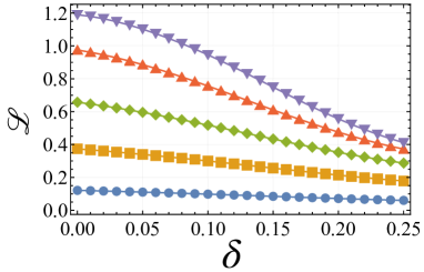
Figure 3: Plots of the $\delta$-dependence of the thermodynamic length $\mathcal{L}$ for $\epsilon=0.01$, $c_{\mathrm{L}}=c_{\mathrm{R}}=1.0$, $r_{\lambda}=r_{\mathrm{L}}=r_{\mathrm{R}}=0.1,0.3,0.5,0.7,0.9$ corresponding to circle, square, diamond, up triangle and down triangle, respectively.

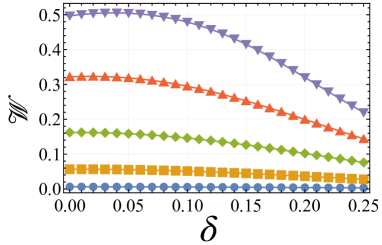
Figure 4: Plots of the $\delta$-dependence of the adiabatic work $\mathcal{W}$ for $\epsilon=0.01$, $c_{\mathrm{L}}=c_{\mathrm{R}}=1.0$, $r_{\lambda}=r_{\mathrm{L}}=r_{\mathrm{R}}=0.1,0.3,0.5,0.7,0.9$ corresponding to circle, square, diamond, up triangle and down triangle, respectively.

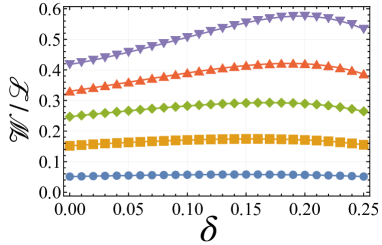
Figure 5: Plots of the $\delta$-dependence of the ratio $\mathcal{W}/\mathcal{L}$ for $\epsilon=0.01$, $c_{\mathrm{L}}=c_{\mathrm{R}}=1.0$, $r_{\lambda}=r_{\mathrm{L}}=r_{\mathrm{R}}=0.1,0.3,0.5,0.7,0.9$ corersponding to circle, square, diamond, up triangle and down triangle, respectively.

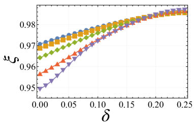
Figure 6: Plots of the $\delta$-dependence of the effective efficiency $\xi$ for $\epsilon=0.01$, $c_{\mathrm{L}}=c_{\mathrm{R}}=1.0$, $r_{\lambda}=r_{\mathrm{L}}=r_{\mathrm{R}}=0.1,0.3,0.5,0.7,0.9$ corresponding to circle, square, diamond, up triangle and down triangle, respectively.

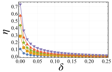
Figure 7: Plots of the $\delta$-dependence of the thermal efficiency $\eta$ for $\epsilon=0.01$, $c_{\mathrm{L}}=c_{\mathrm{R}}=1.0$, $r_{\lambda}=r_{\mathrm{L}}=r_{\mathrm{R}}=0.1,0.3,0.5,0.7,0.9$ corresponding to circle, square, diamond, up triangle and down triangle, respectively.

IV CONCLUSION

In this paper, we successfully extended the geometrical thermodynamics formulated in Refs. Brandner-Saito and engine to a system coupled to two slowly modulated reservoirs, i.e. the adiabatic (Thouless) pumping system without average bias. In the adiabatic regime, the extracted work can be written as the line integral Eq. (39) of the thermodynamic vector potential Eq. (40) along the path of the manipulation in the parameter space. On the other hand, the lower bound of the dissipated availability can be written as the thermodynamic length (37) along the path. By using these results, we obtained the geometrical trade-off relation (43) between the power and effective efficiency in the adiabatic limit. We applied these results to a two-level spin-boson system to obtain the explicit values of the power and effective efficiency. In contrast to Ref. engine , we have analyzed a pumping system with two reservoirs of the same average temperature. Thanks to this setup, the geometrical contribution plays the dominant role in the thermodynamics of the heat engine.

Our future tasks are as follows: (i) To calculate the thermodynamic metric or vector potential, we need to know the explicit form of the steady state of the master equation. In other words, our method cannot be used to systems for which a steady solution cannot be explicitly obtained. Because nonequilibrium steady solutions cannot be obtained in most nonequilibrium systems, we need to extend our formulation even if the steady solution cannot be obtained. (ii) The relationship between the effective efficiency $\xi$ and the conventional thermal efficiency $\eta:=W/Q_{\mathrm{in}}$ is unclear in general systems. Clarifying this relationship is our future work. (iii) In order to optimize the heat engine, one should find a trajectory that maximizes the ratio $\mathcal{W}/\mathcal{L}$ which could not be determined even in the spin-boson model in Sec. III. The configuration of such an optimal trajectory is our future work. (iv) Because the present method is restricted to the adiabatic case $\epsilon\to 0$, at least, for the argument after Sec. II.3, we will need to extend the analysis to the non-adiabatic regime for finite $\epsilon$. Reference FHHT obtained the non-adiabatic solution of a classical master equation and geometrical representation of the non-adiabatic current in two level system. We expect to apply these methods to investigate the non-adiabatic effect in heat engines. (v) Because we only focus on a classical system, we will have to try to extend our analysis to quantum systems in which quantum coherence plays an important role. Reference Brandner-Saito showed that quantum coherence reduces the performance of slowly driven heat engines. On the other hand, it was shown that coherence can enhance the performance of heat engines in Ref. coherence . Therefore, we will have to analyze full quantum systems to clarify whether the coherence can improve the efficiency in the heat engine undergoing an adiabatic pumping process.

Appendix A Slow-driving perturbation

In this appendix, we explain the outline of the perturbation theory of the master equation with slowly modulated parameters slow_dynamics . First, we expand the solution of Eq. (1) in terms of $\epsilon$ as

$$|p(\theta)\rangle=\sum_{n=0}^{\infty}\epsilon^{n}|p^{(n)}(\bm{\Lambda}(\theta))\rangle.$$ (71)

Since the normalization condition $\langle 1|p(\theta)\rangle=1$ holds for any $\epsilon$, $|p^{(n)}(\bm{\Lambda}(\theta))\rangle$ satisfies

$$\langle 1|p^{(0)}(\bm{\Lambda}(\theta))\rangle=1,$$ (72)

$$\langle 1|p^{(n)}(\bm{\Lambda}(\theta))\rangle=0\;(n\geq 1).$$ (73)

Substituting these into Eq. (1), we obtain

$$\hat{K}(\bm{\Lambda}(\theta))|p^{(0)}(\bm{\Lambda}(\theta))\rangle=0,$$ (74)

$$\hat{K}(\bm{\Lambda}(\theta))|p^{(n)}(\bm{\Lambda}(\theta))\rangle=\frac{d}{d\theta}|p^{(n-1)}(\bm{\Lambda}(\theta))\rangle\;(n\geq 1).$$ (75)

Equation (74) means that $|p_{0}(\bm{\Lambda}(\theta))\rangle$ is the instantaneous steady state of $\hat{K}(\bm{\Lambda}(\theta))$:

$$|p^{(0)}(\bm{\Lambda}(\theta))\rangle=|p^{\mathrm{ss}}(\bm{\Lambda}(\theta))\rangle.$$ (76)

By using the pseudo-inverse $\hat{K}^{+}(\bm{\Lambda}(\theta))$ of $\hat{K}(\bm{\Lambda}(\theta))$, Eq. (75) can be written as

$$|p^{(n)}(\bm{\Lambda}(\theta))\rangle =\hat{K}^{+}(\bm{\Lambda}(\theta))\frac{d}{d\theta}|p^{(n-1)}(\bm{\Lambda}(\theta))\rangle$$

$$=\left(\hat{K}^{+}(\bm{\Lambda}(\theta))\frac{d}{d\theta}\right)^{n}|p^{\mathrm{ss}}(\bm{\Lambda}(\theta))\rangle.$$ (77)

Ignoring terms of $O(\epsilon^{2})$ and higher in Eq. (71), we obtain Eq. (24) of the main text.

Appendix B Pseudo-inverse of the transition matrix

In this appendix, we introduce the pseudo-inverse $\hat{K}^{+}(\bm{\Lambda})$ of $\hat{K}(\bm{\Lambda})$, which satisfies following conditions inverse ; Mandal

$$\hat{K}^{+}(\bm{\Lambda})\hat{K}(\bm{\Lambda})=1-|p^{\mathrm{ss}}(\bm{\Lambda})\rangle\langle 1|,$$ (78)

$$\hat{K}(\bm{\Lambda})\hat{K}^{+}(\bm{\Lambda})=1-|p^{\mathrm{ss}}(\bm{\Lambda})\rangle\langle 1|,$$ (79)

$$\hat{K}^{+}(\bm{\Lambda})|p^{\mathrm{ss}}(\bm{\Lambda})\rangle=0,$$ (80)

$$\langle 1|\hat{K}^{+}(\bm{\Lambda})=0.$$ (81)

In particular, if $\hat{K}(\bm{\Lambda})$ is diagonalizable, $\hat{K}(\bm{\Lambda})=\sum_{m}\phi_{m}(\bm{\Lambda})|r_{m}(\bm{\Lambda})\rangle\langle l_{m}(\bm{\Lambda})|$, $\hat{K}^{+}(\bm{\Lambda})$ can be written as

$$\hat{K}^{+}(\bm{\Lambda})=\sum_{m\neq 0}\phi_{m}(\bm{\Lambda})^{-1}|r_{m}(\bm{\Lambda})\rangle\langle l_{m}(\bm{\Lambda})|,$$ (82)

where $\phi_{m}(\bm{\Lambda})$ is the eigenvalue and $|r_{m}(\bm{\Lambda})\rangle$, $\langle l_{m}(\bm{\Lambda})|$ are the corresponding right and left eigenvectors of $\hat{K}(\bm{\Lambda})$. Here we note that $\phi_{0}(\bm{\Lambda})=0$, then $|r_{0}(\bm{\Lambda})\rangle=|p^{\mathrm{ss}}(\bm{\Lambda})\rangle$ and $\langle l_{0}(\bm{\Lambda})|=\langle 1|$. Here we assume that these eigenstates do not degenerate.

As we mentioned in Sec. II.3, the pseudo-inverse $\hat{K}^{+}(\bm{\Lambda})$ can be also written as Eq. (26). We can easily check that the form of the pseudo-inverse in Eq. (26) also satisfies the above conditions (78) - (81).

Appendix C Spin-Boson model

In this appendix, we summerize the detailed setup of the spin-boson model used in Sec. III.

In the spin-boson model, the total Hamiltonian is given by $H_{\mathrm{tot}}=H_{\mathrm{S}}+\sum_{\nu=\mathrm{L},\mathrm{R}}[H_{\alpha}+H_{S\alpha}]$. Each term is given by

$$H_{\mathrm{S}}=\frac{\hbar\omega_{0}}{2}\sigma_{z},$$ (83)

$$H_{\alpha}=\sum_{k}\hbar\omega_{k,\nu}b_{k,\alpha}^{\dagger}b_{k,\alpha},$$ (84)

$$H_{\mathrm{S}\alpha}=\hbar\sigma_{x}\otimes\sum_{k}g_{k,\alpha}(b_{k,\alpha}+b_{k,\alpha}^{\dagger}),$$ (85)

where $\hbar\omega_{0}$ is the energy gap between the two levels in the target system. $\sigma_{z}$ and $\sigma_{x}$ are Pauli operators, where $\omega_{k,\nu}$ is the angular frequency at wave number $k$ for the $\alpha$-th reservoir and $b_{k,\alpha}$ ( $b_{k,\alpha}^{\dagger}$) is the boson annihilation (creation) operator for the $\alpha$-th reservoir, respectively. Here $g_{k,\alpha}$ is the coupling constant, which is related to the spectral density function $D_{\alpha}(\omega):=2\pi\sum_{k}g_{k,\alpha}^{2}\delta(\omega-\omega_{k,\alpha})$. For later analysis, we use the line-width $\Gamma^{\alpha}=D^{\alpha}(\omega)$ which is independent of $\omega$.

We assume that the bosonic reservoirs are always at equilibrium. Thus, the density matrix of the $\nu-$th reservoir is expressed as $\rho_{\alpha}^{\mathrm{eq}}(\beta^{\alpha})=e^{-\beta^{\alpha}H_{\alpha}}/Z_{\alpha}$ at the inverse temperature $\beta^{\alpha}$, where $Z_{\alpha}=\mathrm{Tr}_{\alpha}[e^{-\beta^{\alpha}H_{\alpha}}]$.

The total density matrix $\rho_{\mathrm{tot}}(t)$ follows von-Neumann equation. Under Born-Markov approximation, the reduced dynamics of the target system $\rho(t):=\mathrm{Tr}_{\mathrm{L,R}}[\rho_{\mathrm{tot}}(t)]$ can be describe by the Lindblad master equation Breuer . Moreover, the diagonal part of $\rho(t)$ is described by the master equation:

$$\frac{d}{dt}\left(\begin{array}[]{c}p_{0}(t)\\ p_{1}(t)\end{array}\right)=\sum_{\alpha=\mathrm{L,R}}\left(\begin{array}[]{cc}-\Gamma^{\alpha}n^{\alpha}&\Gamma^{\alpha}(1+n^{\alpha})\\ \Gamma^{\alpha}n^{\alpha}&-\Gamma^{\alpha}(1+n^{\alpha})\end{array}\right)\left(\begin{array}[]{c}p_{0}(t)\\ p_{1}(t)\end{array}\right),$$ (92)

where $n^{\alpha}$ is the Bose distribution function in reservoir $\alpha$ given by

$$n^{\alpha}:=\frac{1}{e^{\beta^{\alpha}\hbar\omega_{0}}-1}.$$ (93)

By using $\theta:=t/\tau_{\mathrm{p}}$ and $\epsilon:=1/\tau_{\mathrm{p}}\Gamma$ with $\Gamma:=\sum_{\alpha}\Gamma^{\alpha}/2$, we obtain the normalized master equation with (49).

In this model, we control $\beta^{\mathrm{L}}$, $\beta^{\mathrm{R}}$ and $\omega_{0}$. In Sec. III, we have used the notation $E:=\bar{\omega}_{0}:=\int^{1}_{0}d\theta\omega_{0}(\theta)$ and $\lambda(\theta):=\omega(\theta)/\bar{\omega}_{0}$.

References

- (1) D. J. Thouless, Quantization of particle transport, Phys. Rev. B 27, 6083 (1983).
- (2) Q. Niu and D. J. Thouless, Quantised adiabatic charge transport in the presence of substrate disorder and many-body interaction, J. Phys. A : Math. Gen. 17, 2453 (1984).
- (3) M. V. Berry, Quantal phase factors accompanying adiabatic changes, Proc. R. Soc. London Ser. A 392, 45 (1984).
- (4) D. Xiao, M.-C. Chang, and Q. Niu, Berry phase effects on electronic properties, Rev. Mod. Phys. 82, 1959 (2010).
- (5) L. P. Kouwenhoven, A. T. Johnson, N. C. van der Vaart, C. J. P. M. Harmans, and C. T. Foxon, Quantized current in a quantum-dot turnstile using oscillating tunnel barriers,Phys. Rev. Lett. 67, 1626 (1991).
- (6) H. Pothier, P. Lafarge, C. Urbina, D. Esteve, and M. H. Devoret, Single-Electron Pump Based on Charging Effects, Europhys. Lett. 17, 249 (1992).
- (7) M. Switkes, C. M. Marcus, K. Campman, and A. C. Gossard, An Adiabatic Quantum Electron Pump, Science 283, 1905 (1999).
- (8) A. Fuhrer, C. Fasth, and L. Samuelson, Single electron pumping in InAs nanowire double quantum dots, Appl. Phys. Lett. 91, 052109 (2007).
- (9) B. Kaestner, V. Kashcheyevs, G. Hein, K. Pierz, U. Siegner, and H. W. Schumacher, Robust single-parameter quantized charge pumping, Appl. Phys. Lett. 92, 192106 (2008).
- (10) S. J. Chorley, J. Frake, C. G. Smith, G. A. C. Jones, and M. R. Buitelaar, Quantized charge pumping through a carbon nanotube double quantum dot, Appl. Phys. Lett. 100, 143104 (2012).
- (11) S. Nakajima, T. Tomita, S. Taie, T. Ichinose, H. Ozawa, L. Wang, M. Troyer and Y. Takahashi, Topological Thouless pumping of ultracold fermions, Nature Physics 12, 296 (2016).
- (12) M. Lohse, C. Schweizer, O. Zilberberg, M. Aidelsburger and I. Bloch, A Thouless quantum pump with ultracold bosonic atoms in an optical superlattice, Nature Physics 12, 350 (2016).
- (13) S. K. Watson, R. M. Potok, C. M. Marcus, and V. Umansky, Experimental Realization of a Quantum Spin Pump, Phys. Rev. Lett. 91, 258301 (2003).
- (14) P. W. Brouwer, Scattering approach to parametric pumping, Phys. Rev. B 58, R10135 (1998).
- (15) N. A. Sinitsyn and I. Nemenman, The Berry phase and the pump flux in stochastic chemical kinetics, Europhys. Lett. 77, 58001 (2007) .
- (16) N. A. Sinitsyn and I. Nemenman, Universal Geometric Theory of Mesoscopic Stochastic Pumps and Reversible Ratchets, Phys. Rev. Lett. 99, 220408 (2007).
- (17) J. E. Avron, A. Elgart, G. M. Graf, and L. Sadun, Geometry, statistics, and asymptotics of quantum pumps, Phys. Rev. B 62, R10618 (2000).
- (18) M. Moskalets and M. Büttiker, Effect of inelastic scattering on parametric pumping, Phys. Rev. B 64, 201305(R) (2001).
- (19) J. N. H. J. Cremers and P. W. Brouwer, Dephasing in a quantum pump, Phys. Rev. B 65, 115333 (2002).
- (20) A. Andreev and A. Kamenev, Counting Statistics of an Adiabatic Pump, Phys. Rev. Lett. 85, 1294 (2000).
- (21) Y. Makhlin and A. D. Mirlin, Counting Statistics for Arbitrary Cycles in Quantum Pumps, Phys. Rev. Lett. 87, 276803 (2001).
- (22) I. L. Aleiner and A. V. Andreev, Adiabatic Charge Pumping in Almost Open Dots, Phys. Rev. Lett. 81, 1286 (1998).
- (23) E. R. Mucciolo, C. Chamon, and C. M. Marcus, Adiabatic Quantum Pump of Spin-Polarized Current, Phys. Rev. Lett. 89, 146802 (2002).
- (24) J. M. R. Parrondo, Reversible ratchets as Brownian particles in an adiabatically changing periodic potential, Phys. Rev. E 57, 7297 (1998).
- (25) O. Usmani, E. Lutz, and M. Büttiker, Noise-assisted classical adiabatic pumping in a symmetric periodic potential, Phys. Rev. E 66, 021111 (2002).
- (26) R. D. Astumian, Adiabatic Pumping Mechanism for Ion Motive ATPases, Phys. Rev. Lett. 91, 118102 (2003).
- (27) R. D. Astumian, Adiabatic operation of a molecular machine, Proc. Natl. Acad. Sci. USA 104, 19715 (2007).
- (28) S. Rahav, J. Horowitz, and C. Jarzynski, Directed Flow in Nonadiabatic Stochastic Pumps, Phys. Rev. Lett. 101, 140602 (2008).
- (29) V. Y. Chernyak, J. R. Klein, and N. A. Sinitsyn, Quantization and fractional quantization of currents in periodically driven stochastic systems. I. Average currents, J. Chem. Phys. 136, 154107 (2012).
- (30) V. Y. Chernyak, J. R. Klein, and N. A. Sinitsyn, Quantization and fractional quantization of currents in periodically driven stochastic systems. II. Full counting statistics, J. Chem. Phys. 136, 154108 (2012).
- (31) J. Ren, P. Hänggi, and B. Li, Berry-Phase-Induced Heat Pumping and Its Impact on the Fluctuation Theorem, Phys. Rev. Lett. 104, 170601 (2010).
- (32) T. Sagawa and H. Hayakawa, Geometrical expression of excess entropy production, Phys. Rev. E 84, 051110 (2011).
- (33) F. Renzoni and T. Brandes, Charge transport through quantum dots via time-varying tunnel coupling, Phys. Rev. B 64, 245301 (2001).
- (34) T. Brandes and T. Vorrath, Adiabatic transfer of electrons in coupled quantum dots, Phys. Rev. B 66, 075341 (2002).
- (35) E. Cota, R. Aguado, and G. Platero, ac-Driven Double Quantum Dots as Spin Pumps and Spin Filters, Phys. Rev. Lett. 94, 107202 (2005).
- (36) J. Splettstoesser, M. Governale, J. König, and R. Fazio, Adiabatic pumping through a quantum dot with coulomb interactions: A perturbation expansion in the tunnel coupling, Phys. Rev. B 74, 085305 (2006).
- (37) T. Yuge, T. Sagawa, A. Sugita, and H. Hayakawa, Geometrical pumping in quantum transport: Quantum master equation approach, Phys. Rev. B 86, 235308 (2012).
- (38) T. Yuge, T. Sagawa, A. Sugiura, and H. Hayakawa, Geometrical Excess Entropy Production in Nonequilibrium Quantum Systems, J. Stat. Phys. 153, 412 (2013).
- (39) K. L. Watanabe and H. Hayakawa, Geometric fluctuation theorem for a spin-boson system, Phys. Rev. E 96, 022118 (2017).
- (40) Y.Hino and H. Hayakawa, Fluctuation relations for adiabatic pumping, Phys. Rev. E 120, 012115 (2020).
- (41) K. Takahashi, Y. Hino, K. Fujii and H. Hayakawa, Full Counting Statistics and Fluctuation?Dissipation Relation for Periodically Driven Two-State Systems, J. Stat. Phys. 181, 2206 (2020).
- (42) B. Andresen, Finite-time thermodynamics and thermodynamic length, Rev. Gén. Therm. 35, 647 (1996).
- (43) F. Weinhold, Metric geometry of equilibrium thermodynamics, J. Chem. Phys. 63, 2479 (1975).
- (44) G. Ruppeiner, Thermodynamics: A Riemannian geometric model, Phys. Rev. A 20, 1608 (1979).
- (45) P. Salamon and R. S. Berry, Thermodynamic Length and Dissipated Availability, Phys. Rev. Lett. 51, 1127 (1983).
- (46) F. Schlögl, Thermodynamic metric and stochastic measures, Z. Phys. B 59, 449 (1985).
- (47) G. Ruppeiner, Riemannian geometry in thermodynamic fluctuation theory, Rev. Mod. Phys. 67, 605 (1995).
- (48) G. E. Crooks, Measuring Thermodynamic Length, Phys. Rev. Lett. 99, 100602 (2007).
- (49) S. Deffner and E. Lutz, Thermodynamic length for far-from-equilibrium quantum systems, Phys. Rev. E 87, 022143 (2013).
- (50) M. Scandi and M. Perarnau-Llobet, Thermodynamic length in open quantum systems, Quantum 3, 197 (2019).
- (51) K. Brandner and K. Saito, Thermodynamic Geometry of Microscopic Heat Engines Kay Brandner and Keiji Saito, Phys. Rev. Lett. 124, 040602 (2020).
- (52) S. K. Giri and H. P. Goswami, Geometric phaselike effects in a quantum heat engine, Phys. Rev. E 96, 052129 (2017), ibid 99, 022104 (2019).
- (53) T. Hatano and S.-i. Sasa, Steady-State Thermodynamics of Langevin Systems, Phys. Rev. Lett. 86, 3463 (2001).
- (54) T. L. Boullion and P. L. Odell, Generalized Inverse Matrices (Wiley-Interscience, New York,1971).
- (55) K Takahashi, K Fujii, Y Hino, and H Hayakawa, Nonadiabatic Control of Geometric Pumping, Phys. Rev. Lett. 124, 150602 (2020).
- (56) A. A. Svidzinsky, K. E. Dorfman, M. O. Scully, Enhancing photocell power by noise-induced coherence, Coherent Opt. Phenomena, 1, 7 (2012).
- (57) V. Cavina, A. Mari, and V. Giovannetti, Slow Dynamics and Thermodynamics of Open Quantum Systems, Phys. Rev. Lett. 119, 050601 (2017).
- (58) D. Mandal and C. Jarzynski, Analysis of slow transitions between nonequilibrium steady states, J. Stat. Mech. 063204 (2016).
- (59) H. P. Breuer and F. Petruccione, The Theory of Open Quantum Systems (Oxford Univ. Press, Oxford, 2002).