Half-hypermultiplets and incomplete/complete resolutions in F-theory

Abstract

We consider resolutions of codimension-two enhanced singularities from $SO(12)$ to $E_{7}$ and from $E_{7}$ to $E_{8}$ in six-dimensional F-theory, where a half-hypermultiplet arises for generic complex structures achieving them. The exceptional fibers at the enhanced point exhibit different structures depending on how the colliding 7-brane approaches the stack of gauge 7-branes, as previously observed by Morrison and Taylor in the case of the enhancement from $SU(6)$ to $E_{6}$. When the colliding brane approaches them as $O(s)$, where $s$ is the coordinate of the base space along the gauge 7-branes, the resolution process ends up with fewer exceptional fibers than naively expected from the Kodaira classification, with a non-Dynkin intersection matrix including half-integral intersection numbers. We confirm that the exceptional fibers at the enhanced point form extremal rays of the cone of the positive weights of the relevant pseudo-real representation, explaining why a half-hypermultiplet arises there. By altering the ordering of the singularities blown up in the process, we obtain, for both $SO(12)\rightarrow E_{7}$ and $E_{7}\rightarrow E_{8}$, the intersection diagram on every other row of the corresponding box graphs. We present detailed derivations of the intersection diagrams of the exceptional fibers at the singularity enhanced points by examining how an exceptional curve is lifted up on the chart arising due to the subsequent blowing-up process. When the colliding brane approaches the stack of branes as $O(s^{2})$, we obtain additional conifold singularity at the enhanced point, which completes the full Dynkin diagram of the enhanced group as was found previously.

1 Introduction

The significance of F-theory Vafa in modern particle physics model building cannot be overestimated. The characteristic features of the Standard Model can be naturally explained by the $SU(5)$ and $SO(10)$ grand unified theories, which are engineered in F-theory. It can achieve matter fields in the spinor representation as well as the exceptional group gauge symmetry. F-theory has an advantage over the $E_{8}\times E_{8}$ heterotic string theory in that it can address the issue of the gauge/gravity coupling correlation in the latter Witten96 . F-theory can also generate up-type Yukawa couplings perturbatively forbidden in D-brane models Dbranemodels1 ; Dbranemodels2 .

In F-theory, matter typically arises at codimension-two singularities MV1 ; MV2 ; BIKMSV ; KatzVafa ; Tani in the base space of the elliptic fibration. To be specific, consider a six-dimensional F-theory compactified on an elliptically fibered three-fold defined by a hypersurface $\Phi(x,y,z,s)=0$ in $\hbox{\mybbsmall C}^{4}\ni(x,y,z,s)$ over a complex two-fold with local coordinates $(z,s)\in\hbox{\mybbsmall C}^{2}$. Over a generic point with fixed $(z,s)$, this equation describes a genus-one curve. We assume that this hypersurface has a codimension-one singularity of some compact group $H$ along $z=0$ for generic $s\neq 0$, which is enhanced to some compact group $G\supset H$ at a codimension-two particular locus along the line $z=0$, say, at $s=0$.

In this set-up, one typically obtains chiral matter hypermultiplets corresponding to the homogeneous Kähler manifold $G/(H\times U(1))$ MV1 ; MV2 ; BIKMSV ; KatzVafa ; Tani ; FFamilyUnification at the enhanced singularity. However, if $G$ and $H$ are such that

$$G \supset H\times SU(2)$$

dim$$G = (\mbox{\bf dim\boldmath$H$},{\bf 1})\oplus({\bf 2n},{\bf 2})\oplus({\bf 1},{\bf 3}),$$ (1)

where $n=10$, $16$, $28$ for $(G,H)=(E_{6},SU(6))$, $(E_{7},SO(12))$, $(E_{8},E_{7})$, respectively, the matter arising there are not the full hypermultiplets but half-hypermultiplets for generic complex structures achieving such singularities.

In all the cases above, ${\bf 2n}$ is a pseudo-real representation of $H$, of which the representation matrix can be written as an $Sp(2n)$ matrix. For these representations, one can impose the symplectic Majorana condition on the $2n$ complex spinors. One can also define a similar relation among $2n$ pairs of the complex scalars by using a $U(1)_{R}$ rotation. In this way, the degrees of freedom of hypermultiplets are halved, yielding half-hypermultiplets in these representations.

In MT , the resolution of a codimension-two enhancement from $SU(6)$ to $E_{6}$ was studied in six dimensions. It was shown there that, if the colliding brane approaches $z=0$ like $O(s)$ which is the generic case, only five exceptional curves appear through the blowing-up process even at the singularity enhanced point. This type of resolution was called the incomplete resolution in MT . Note that, by resolving a codimension-one $E_{6}$ singularity, one obtains six exceptional fibers consisting the $IV^{*}$ fiber type of Kodaira.

This means that there are not enough new degrees of freedom arising at the enhanced point to generate matter in a full hypermultiplet. The five exceptional fibers form a curious non-Dynkin intersection diagram, however. In particular, some of the exceptional curves turn out to have self-intersection number $-\frac{3}{2}$. This is equal to the minus of the length squared of a weight of the 20 representation. One can verify that these five exceptional curves form extremal rays of the cone of the positive weights of the 20 representation. (Actually, one can show that there are just 20 integer linear combinations of these exceptional curves which have self-intersection number $-\frac{3}{2}$; half of them have positive coefficients and the other half have negative coefficients, giving a whole set of the weights of ${\bf 20}$.) Thus the matter forms a single ${\bf 20}$ representation of $SU(6)$. This shows the mechanism of how the half-hypermultiplet appears in this codimension-two singularity enhancement. (Note that for a full hypermultiplet one needs two ${\bf 20}$ representations, either one of which survives as massless matter in six dimensions.)

On the other hand, if the brane collides like $O(s^{2})$, an extra singularity arises at the intersection. This is a conifold singularity. Resolving it yields another exceptional curve, completing the proper Dynkin intersection diagram expected from the ordinary Kodaira classification. This was called the complete resolution MT .

Higher codimension singularities were also studied in BoxGraphs by exploring the phases of three-dimensional gauge theory arising from the compactification of M-theory on a Calabi-Yau four-fold (see EsoleYau ; MarsanoSSNameki ; EsoleShaoYau ; BraunNameki ). In this approach, the generation of a half-hypermultiplet was explained as a result of the reduction of the massless states occurring due to the monodromy among the fibers BoxGraphs . It was noted there that if the complex structure was tuned so that there were extra sections, the monodromy was reduced and a full hypermultiplet appeared.

In this paper, we study the resolutions of the other two cases, $SO(12)\rightarrow E_{7}$ and $E_{7}\rightarrow E_{8}$, of the codimension-two singularity enhancement in which half-hypermultiplets appear as massless states at the singularity. The strategy is the same as that used in MT . To blow up this singularity along the line $z=0$ we replace the local ambient space $\hbox{\mybbsmall C}^{4}$ with

$${\widehat{\hbox{\mybbsmall C}}}^{4} = \left\{\left.((x,y,z,s);(\xi:\eta:\zeta))\in\hbox{\mybbsmall C}^{4}\times\hbox{\mybbsmall P}^{2}\right|x\eta-y\xi=y\zeta-z\eta=z\xi-x\zeta=0\right\}$$ (2)

and consider the hypersurface in it. (2) inserts a continuous family of $\hbox{\mybbsmall P}^{2}$ along the complex line $z=0$ for arbitrary $s\in\hbox{\mybbsmall C}$. Then we find that there still are several, (again) codimension-one singularities on the intersection of ${\widehat{\hbox{\mybbsmall C}}}^{4}$ (2) and the hypersurface $\Phi=0$. To resolve these singularities, we further make a replacement similar to $\hbox{\mybbsmall C}^{4}\rightarrow{\widehat{\hbox{\mybbsmall C}}}^{4}$ along each singular line and consider the hypersurface in this blown-up ambient space. Then if we still find some singularities of codimension one, we perform a codimension-one blow up along each of them. Repeating these steps we end up with either of the two cases:
(1) The case where there are no more singularities of any kind on the final hypersurface.
(2) The case where there are no more codimension-one singularities, but still there is an isolated codimension-two singularity at $s=0$ on the final hypersurface.

This is the phenomenon known as the partial simultaneous resolution of singularities PSR1 ; PSR2 ; KatzMorrison ; BoxGraphs , and which case we will end up with depends on the vanishing order of the relevant section of the projective-space bundle for the respective singularity enhancement. For the enhancement $SU(6)\rightarrow E_{6}$ studied in MT , the relevant section is the polynomial $t_{r}(s)$ in eq.(8) (see below), for $SO(12)\rightarrow E_{7}$ it is $H_{n+4}(s)$, and for $E_{7}\rightarrow E_{8}$ it is $f_{n+8}(s)$. We will show that, also for the cases $SO(12)\rightarrow E_{7}$ and $E_{7}\rightarrow E_{8}$ we will consider in this paper, we are led to the result (1) if these sections vanish like $O(s)$ as $s\rightarrow 0$. The codimension-two singularity is then resolved only by the codimension-one blow-ups in the ambient space, and therefore the number of times of the blowing-up operations is the same as that needed to resolve a Kodaira $H$ singularity for fixed generic $s\neq 0$. Thus there are not enough exceptional curves to form the proper Dynkin diagram of $G$ as their intersection matrix. Even so, we will see that the intersection diagram of the exceptional curves obtained by the $s\rightarrow 0$ limit of the exceptional surfaces is different from the Dynkin diagram of $H$. Rather, it turns out that some of the curves have their self-intersection number $-\frac{3}{2}$, as was observed in MT for the $SU(6)\rightarrow E_{6}$ enhancement.

We perform blowing-ups for all possible inequivalent orderings of blowing up the singularities in both the enhancements $SO(12)\rightarrow E_{7}$ and $E_{7}\rightarrow E_{8}$. We find that the intersection diagram on every other row in Figures 33 and 44 of BoxGraphs can be obtained, but not all of them. Although the intersection diagrams are different, the fibers obtained in the limit $s\rightarrow 0$ always form extremal rays of the cone of the positive weights of the relevant pseudo-real representation.

On the other hand, if they vanish like $O(s^{2})$, we are led to the result (2), where we need a further resolution of the isolated singularity. This is the complete resolution; we have one more additional node to the incomplete intersection diagram obtained in the incomplete resolution, obtaining the full Dynkin diagram of the group $G$. We will find that, as was observed in MT , this final singularity appearing at codimension two is a conifold singularity for all the cases we examine in this paper.

The plan of this paper is as follows. In section 2, we review in what circumstances massless matter fields appear as half-hypermultiplets in the global six-dimensional F-theory compactification on an elliptic Calabi-Yau three-fold over a Hirzebruch surface. In section 3, we present the detailed process of blow-ups for the codimension-two singularity enhancement from $SO(12)$ to $E_{7}$. In section 4, we turn to the resolution of the enhancement from $E_{7}$ to $E_{8}$. Section 5 summarizes the conclusions. In Appendix A, we explain the relations between symplectic Majorana-Weyl spinors, pseudo-real representations and half-hypermultiplets. In Appendix B, we summarize the results of MT on the resolution of the enhancement $SU(6)\rightarrow E_{6}$. Finally, in Appendix C, we present a basic explanation of the small resolution of a conifold.

2 Half-hypermultiplets in six-dimensional F-theory

Half-hypermultiplets arise when the unbroken gauge group is $SU(6)$, $SO(12)$ or $E_{7}$ BIKMSV . These models can be systematically obtained by tuning the complex structure of the $SU(5)$ model.

We start with the six-dimensional compactification on F-theory on an elliptically fibered Calabi-Yau three-fold over a Hirzebruch surface $\hbox{\mybbsmall F}_{n}$ MV1 ; MV2 . Let $z$, $z^{\prime}$ be affine coordinates of the fiber and base $\hbox{\mybbsmall P}^{1}$’s, respectively. The Weierstrass model

$$y^{2}=x^{3}+f(z,z^{\prime})x+g(z,z^{\prime})$$ (3)

develops an $SU(5)$ singularity if BIKMSV

$$f(z,z^{\prime}) = -3h_{n+2}^{4}+12h_{n+2}^{2}H_{n+4}z-12\left(H_{n+4}^{2}-h_{n+2}q_{n+6}\right)z^{2}+f_{n+8}z^{3}+f_{8}z^{4},$$

$$g(z,z^{\prime}) = 2h_{n+2}^{6}-12h_{n+2}^{4}H_{n+4}z+\left(24h_{n+2}^{2}H_{n+4}^{2}-12h_{n+2}^{3}q_{n+6}\right)z^{2}$$ (4)

$$+\left(-f_{n+8}h_{n+2}^{2}+24h_{n+2}H_{n+4}q_{n+6}-16H_{n+4}^{3}\right)z^{3}$$

$$+\left(-f_{8}h_{n+2}^{2}+2f_{n+8}H_{n+4}+12q_{n+6}^{2}\right)z^{4}+g_{n+12}z^{5}+g_{12}z^{6},$$

where $h_{n+2}$,$H_{n+4}$,$q_{n+6}$,$f_{n+8}$ and $g_{n+12}$ are polynomials of $z^{\prime}$ of degrees specified by the subscripts. They are sections of Looijenga’s weighted projective space bundle FMW ; DonagiWijnholt ; MizoguchiTaniLooijenga characterizing the $SU(5)_{\rm instanton}$ vector bundle of the dual heterotic string theory. This Calabi-Yau three-fold admits a $K3$ fibration, and we work with one of the rational elliptic surfaces in the stable degeneration limit of the $K3$ so that the orders of the polynomials $f(z,z^{\prime})$ and $g(z,z^{\prime})$ are truncated at $z^{4}$ and $z^{6}$, respectively. This suffices since the anomalies cancel for each $E_{8}$ gauge group, and also we are interested in the local structure of the singularity. $x$ and $y$ are then taken to be sections of ${\cal O}(2(-K_{\hbox{\mybbsub F}_{n}}-C_{0}))$ and ${\cal O}(3(-K_{\hbox{\mybbsub F}_{n}}-C_{0}))$, where $C_{0}$ is a divisor class with $C_{0}^{2}=-n$, satisfying $-K_{\hbox{\mybbsub F}_{n}}=2C_{0}+(2+n)f$ with the fiber class $f$. Similar modifications are necessary for $f(z,z^{\prime})$ and $g(z,z^{\prime})$. This deviation from the anti-canonical class (and hence from a Calabi-Yau) is because we consider a rational-elliptic-surface fibration.

The Weierstrass equation (3) with (4) can be written in Tate’s form as

$$y^{\prime 2}+x^{\prime 3}+\alpha_{4}z^{4}x^{\prime}+\alpha_{6}z^{6}+a_{0}z^{5}+a_{2}z^{3}x^{\prime}+a_{3}z^{2}y^{\prime}+a_{4}zx^{\prime 2}+a_{5}x^{\prime}y^{\prime}=0$$ (5)

with

$$a_{5}= 2\sqrt{3}ih_{n+2},$$ (6)

$$a_{4}= -6H_{n+4},$$

$$a_{3}= 4\sqrt{3}iq_{n+6},$$

$$a_{2}= f_{n+8},$$

$$a_{0}= g_{n+12}-2H_{n+4}f_{8},$$

$$\alpha_{4}= f_{8},$$

$$\alpha_{6}= g_{12}.$$

For completeness we write $x$, $y$ in (3) in terms of $x^{\prime}$, $y^{\prime}$ in (5):

$$x = x^{\prime}+\frac{1}{3}\left(a_{4}z-\frac{1}{4}a_{5}^{2}\right),$$

$$y = i\left(y^{\prime}+\frac{1}{2}\left(a_{5}x^{\prime}+a_{3}z^{2}\right)\right).$$ (7)

$SU(6)$

To obtain an equation for $SU(6)$ gauge group, which yields half-hypermultiplets, we set BIKMSV

$$h_{n+2} = t_{r}h_{n+2-r},$$

$$H_{n+4} = t_{r}H_{n+4-r},$$

$$q_{n+6} = u_{r+4}h_{n+2-r},$$

$$f_{n+8} = t_{r}f_{n+8-r}-12u_{r+4}H_{n+4-r},$$

$$g_{n+12} = 2(u_{r+4}f_{n-r+8}+f_{8}t_{r}H_{n-r+4}).$$ (8)

Then the spectral cover factorizes as

$$0 = a_{0}z^{5}+a_{2}z^{3}x^{\prime}+a_{3}z^{2}y^{\prime}+a_{4}zx^{\prime 2}+a_{5}x^{\prime}y^{\prime}$$ (9)

$$= \left(x^{\prime}t_{r}+2z^{2}u_{r+4}\right)\left(z^{3}f_{n-r+8}+2i\sqrt{3}y^{\prime}h_{n-r+2}-6zx^{\prime}H_{n-r+4}\right),$$

indicating that the $SU(5)$ instanton is reduced to an $SU(3)\times SU(2)$ instanton in the heterotic dual, at the same time the Mordell-Weil rank of the rational elliptic surface is reduced. The Mordell-Weil lattice is No.15 in the Oguiso-Shioda classification OguisoShioda . In this specification $f(z,z^{\prime})$ and $g(z,z^{\prime})$ become

$$f_{SU(6)}(z,z^{\prime}) = -3t_{r}^{4}h_{n-r+2}^{4}+12zt_{r}^{3}h_{n-r+2}^{2}H_{n-r+4}+z^{2}\left(12t_{r}u_{r+4}h_{n-r+2}^{2}-12t_{r}^{2}H_{n-r+4}^{2}\right)$$ (10)

$$+z^{3}\left(t_{r}f_{n-r+8}-12u_{r+4}H_{n-r+4}\right)+f_{8}z^{4},$$

$$g_{SU(6)}(z,z^{\prime}) = 2t_{r}^{6}h_{n-r+2}^{6}-12zt_{r}^{5}h_{n-r+2}^{4}H_{n-r+4}$$ (11)

$$+z^{2}\left(24t_{r}^{4}h_{n-r+2}^{2}H_{n-r+4}^{2}-12t_{r}^{3}u_{r+4}h_{n-r+2}^{4}\right)$$

$$+z^{3}\left(-t_{r}^{3}f_{n-r+8}h_{n-r+2}^{2}+36t_{r}^{2}u_{r+4}h_{n-r+2}^{2}H_{n-r+4}-16t_{r}^{3}H_{n-r+4}^{3}\right)$$

$$+z^{4}\left(-f_{8}t_{r}^{2}h_{n-r+2}^{2}+2t_{r}^{2}f_{n-r+8}H_{n-r+4}+12u_{r+4}^{2}h_{n-r+2}^{2}-24t_{r}u_{r+4}H_{n-r+4}^{2}\right)$$

$$+z^{5}\left(2f_{8}t_{r}H_{n-r+4}+2u_{r+4}f_{n-r+8}\right)+g_{12}z^{6}.$$

The discriminant reads

$$\Delta_{SU(6)} = 9z^{6}t_{r}^{3}h_{n-r+2}^{4}\left[t_{r}^{3}\left(12g_{12}h_{n-r+2}^{2}-f_{n-r+8}^{2}\right)\right.$$ (12)

$$~{}~{}~{}~{}~{}~{}~{}~{}~{}~{}~{}~{}~{}~{}~{}~{}+t_{r}^{2}\left(-24f_{8}u_{r+4}h_{n-r+2}^{2}-24u_{r+4}f_{n-r+8}H_{n-r+4}\right)$$

$$~{}~{}~{}~{}~{}~{}~{}~{}~{}~{}~{}~{}~{}~{}~{}~{}\left.-144t_{r}u_{r+4}^{2}H_{n-r+4}^{2}-96u_{r+4}^{3}h_{n-r+2}^{2}\right]+O(z^{7}).$$

Thus the Weierstrass model with (10),(11) indeed has a codimension-one $SU(6)$ singularity along $z=0$.

The zero loci of $t_{r}$ are the points where the $SU(6)$ singularity is enhanced to $E_{6}$, those of $h_{n-r+2}$ are the ones to $D_{6}$, and those of the remaining factor of degree $2n+r+16$ are the ones to $A_{6}$. They respectively yield $r$ half-hypermultiplets in 20, $n-r+2$ hypermultiplets in 15 and $2n+r+16$ hypermultiplets in 6.

The number of the complex structure moduli is $3n-r+21$, which satisfies the anomaly-free constraint for one of the $E_{8}$ factors BIKMSV

$$n_{H}-n_{V} = 20\cdot\frac{r}{2}+15(n-r+2)+6(2n+r+16)+3n-r+21~{}-35$$ (13)

$$= 30n+112.$$

Note that this condition does not hold if the multiplets in 20 are ordinary hypermultiplets.

$SO(12)$

To further obtain an equation for $SO(12)$ gauge group, one only needs to set $h_{n+2-r}=0$ in (8). The spectral cover is now

$$\left(x^{\prime}t_{r}+2z^{2}u_{r+4}\right)\left(x^{\prime}H_{n-r+4}-\frac{1}{6}z^{2}f_{n-r+8}\right) = 0.$$ (14)

These factors are in the same form, corresponding to two $SU(2)$’s of the instanton gauge group of the heterotic theory. The Mordell-Weil lattice is No.26 in OguisoShioda .

Then $f(z,z^{\prime})$ and $g(z,z^{\prime})$ are

$$f_{SO(12)}(z,z^{\prime}) = -12z^{2}t_{r}^{2}H_{n-r+4}^{2}+z^{3}\left(t_{r}f_{n-r+8}-12u_{r+4}H_{n-r+4}\right)+f_{8}z^{4},$$ (15)

$$g_{SO(12)}(z,z^{\prime}) = -16z^{3}t_{r}^{3}H_{n-r+4}^{3}+2z^{4}\left(t_{r}^{2}f_{n-r+8}H_{n-r+4}-12t_{r}u_{r+4}H_{n-r+4}^{2}\right)$$ (16)

$$+2z^{5}\left(f_{8}t_{r}H_{n-r+4}+u_{r+4}f_{n-r+8}\right)+g_{12}z^{6}.$$

The discriminant is

$$\Delta_{SO(12)} = -36z^{8}t_{r}^{2}H_{n-r+4}^{2}\left(t_{r}f_{n-r+8}+12u_{r+4}H_{n-r+4}\right){}^{2}+O(z^{9}).$$ (17)

The zero loci of both $t_{r}$ and $H_{n-r+4}$ give rise to $E_{7}$ singularities to yield $n+4$ half-hypermultiplets. The loci of the remaining factor are $A_{7}$ singularities, giving $n+8$ hypers in 12. With additional neutral hypermultiplets from the $2n+18$ complex structure moduli, we have

$$n_{H}-n_{V} = 32\cdot\frac{n+4}{2}+12(n+8)+2n+18~{}-66$$ (18)

$$= 30n+112$$

as it should be. Again, if 32 is not a half-hyper, the anomaly does not cancel.

$E_{7}$

Finally, the $E_{7}$ model can be obtained by setting $h_{n+2}=H_{n+4}=q_{n+6}=0$ in the $SU(5)$ model. The gauge group of the heterotic vector bundle is $SU(2)$. The Mordell-Weil lattice is No.43 in OguisoShioda . $f(z,z^{\prime})$ and $g(z,z^{\prime})$ are simply given by

$$f_{E_{7}}(z,z^{\prime}) = f_{n+8}z^{3}+f_{8}z^{4},$$ (19)

$$g_{E_{7}}(z,z^{\prime}) = g_{n+12}z^{5}+g_{12}z^{6}.$$ (20)

The discriminant

$$\Delta_{E_{7}} = 4f_{n+8}^{3}z^{9}+O(z^{10})$$ (21)

implies that $n+8$ half-hypermultiplets in 56 of $E_{7}$ arise. Again they must be half-hyper as

$$n_{H}-n_{V} = 56\cdot\frac{n+8}{2}+2n+21~{}-133$$ (22)

$$= 30n+112.$$

3 $SO(12)\rightarrow E_{7}$

We consider a Weierstrass model on a base two-fold $B_{2}$ with local coordinates $\{z,s\}$, where the codimension-one singularity arises along $z=0$ and the codimension-two singularity arises at $s=0$ on the $z=0$ complex line. $s$ corresponds to $z^{\prime}$ in the previous section.

3.1 Incomplete resolution: Blowing up $p_{1}$ first

3.1.1 Blowing up process

We consider a concrete Weierstrass model of incomplete resolution by setting  $H_{n-r+4}=s$, $t_{r}=-\frac{1}{2}$, $f_{n-r+8}=-2$ and $u_{r+4}=f_{8}=g_{12}=0$ in (15) and (16):

$$\Phi(x,y,z,s) = -y^{2}+x^{3}+f(z,s)x+g(z,s)=0,$$ (23)

where

$$f(z,s) = -3s^{2}z^{2}+z^{3},$$

$$g(z,s) = 2s^{3}z^{3}-sz^{4}.$$ (24)

At $s\neq 0$, the orders of $f$, $g$ and the discriminant $\Delta$ in $z$ are $(2,3,8)$, while at $s=0$, they satisfy $(3,\geq 5,9)$. Therefore (24) describes the enhancement $I_{2}^{*}\rightarrow III^{*}$ ($SO(12)\rightarrow E_{7}$) of the Kodaira type, satisfying the requirement.

1st blow up

With (24), the equation (23) reads

$$\Phi(x,y,z,s)=xz^{2}(z-3s^{2})+sz^{3}(2s^{2}-z)+x^{3}-y^{2} = 0.$$ (25)

(25) has a codimension-one singularity at $p_{0}\equiv(0,0,0,s)$. We blow up this by replacing the complex line $(x,y,z)=(0,0,0)$ with $\hbox{\mybbsmall P}^{2}\times\hbox{\mybbsmall C}$ in $\hbox{\mybbsmall C}^{4}$ by passing to the following charts corresponding to three affine patches of $\hbox{\mybbsmall P}^{2}$ for fixed $s$:
Chart $1_{x}$

$$\Phi(x,xy_{1},xz_{1},s) = x^{2}\Phi_{x}(x,y_{1},z_{1},s),$$

$$\Phi_{x}(x,y_{1},z_{1},s) = x^{2}\left(z_{1}^{3}-sz_{1}^{4}\right)+x\left(sz_{1}-1\right)^{2}\left(2sz_{1}+1\right)-y_{1}^{2}.$$

$$\cal C {}_{p_{0}} 1_{x} : x=0,~{}~{}y_{1}=0.$$ in

Singularities $$: (x,y_{1},z_{1},s)=(0,0,\frac{1}{s},s),(0,0,-\frac{1}{2s},s).$$ (26)

These singularities are of codimension one, which we refer to as $p_{1}$ and $q_{1}$, respectively. $\cal C$${}_{p_{0}}$ is the exceptional curve at fixed $s$.

Chart $1_{y}$

$$\Phi(x_{1}y,y,yz_{1},s) = y^{2}\Phi_{y}(x_{1},y,z_{1},s),$$

$$\Phi_{y}(x_{1},y,z_{1},s) = 2s^{3}yz_{1}^{3}+x_{1}yz_{1}^{2}\left(yz_{1}-3s^{2}\right)-sy^{2}z_{1}^{4}+x_{1}^{3}y-1.$$

$$\cal C {}_{p_{0}} 1_{y} :$$ in Invisible in this patch.

Singularities $$:$$ None. (27)

In chart $1_{y}$, the exceptional curve cannot be seen and there is no singularity.

Chart $1_{z}$

$$\Phi(x_{1}z,y_{1}z,z,s) = z^{2}\Phi_{z}(x_{1},y_{1},z,s),$$

$$\Phi_{z}(x_{1},y_{1},z,s) = z\left(2s^{3}-3s^{2}x_{1}-sz+x_{1}^{3}+x_{1}z\right)-y_{1}^{2}.$$

$$\cal C {}_{p_{0}} 1_{z} : z=0,~{}~{}y_{1}=0.$$ in

Singularities $$: (x_{1},y_{1},z,s)=(s,0,0,s),(-2s,0,0,s).$$ (28)

The first singularity is $p_{1}$, while the second is $q_{1}$.

2nd blow up

By the 1st blow up we found two singularities. There are two ways to resolve them; either we blow up $p_{1}$ first, or $q_{1}$ first. In this section we blow up $p_{1}$ first.

In order to blow up the singularity $p_{1}$ in $\Phi_{z}(x_{1},y_{1},z,s)=0$, we shift the coordinate $x_{1}$ so that the position of the singularity becomes $(0,0,0,s)$:

$$\Psi_{z}(\tilde{x}_{1},y_{1},z,s) \equiv \Phi_{z}(\tilde{x}_{1}+s,y_{1},z,s).$$ (29)

The singularities of $\Psi_{z}(\tilde{x}_{1},y_{1},z,s)=0$ are now at $(0,0,0,s)$ $(=p_{1})$ and $(-3s,0,0,s)$ $(=q_{1})$. We blow up the singularity of $\Psi_{z}(\tilde{x}_{1},y_{1},z,s)=0$ at $(0,0,0,s)$.

Chart $2_{zx}$

$$\Psi_{z}(\tilde{x}_{1},\tilde{x}_{1}y_{2},\tilde{x}_{1}z_{2},s) = \tilde{x}_{1}^{2}\Psi_{zx}(\tilde{x}_{1},y_{2},z_{2},s),$$

$$\Psi_{zx}(\tilde{x}_{1},y_{2},z_{2},s) = \tilde{x}_{1}z_{2}(3s+\tilde{x}_{1}+z_{2})-y_{2}^{2}.$$

$$\cal C {}_{p_{1}} 2_{zx} : \tilde{x}_{1}=0,~{}~{}y_{2}=0.$$ in

Singularities $$: (\tilde{x}_{1},y_{2},z_{2},s)=(0,0,0,s)(=p_{2}),(0,0,-3s,s)(=r_{2}),$$ (30)

$$(-3s,0,0,s)(=q_{1}).$$

We find three singularities in this chart and name them as shown in the parentheses.

Chart $2_{zy}$  In this chart, we find no singularity so we omit the details of $\Psi_{zy}$.

Chart $2_{zz}$

$$\Psi_{z}(x_{2}z,y_{2}z,z,s) = z^{2}\Psi_{zz}(x_{2},y_{2},z,s),$$

$$\Psi_{zz}(x_{2},y_{2},z,s) = x_{2}z\left(3sx_{2}+x_{2}^{2}z+1\right)-y_{2}^{2}.$$

$$\cal C {}_{p_{1}} 2_{zz} : z=0,~{}~{}y_{2}=0.$$ in

Singularities $$: (x_{2},y_{2},z,s)=(0,0,0,s)(=q_{2}),(-\frac{1}{3s},0,0,s)(=r_{2}).$$ (31)

We observe two singularities. The former ($q_{2}$) is one which can only be seen in this chart, while the latter ($r_{2}$) is already seen in chart $2_{zx}$.

Here the process branches off in three ways depending on which of the three singularities $p_{2}$, $r_{2}$ and $q_{1}$ in chart $2_{zx}$ is blown up next. Although they are separated for $s\neq 0$, they coincide with each other at $s=0$ (see (30)). For this reason, changing the order of blowing up these three singularities changes the subsequent geometries. In this section, we consider the case $p_{2}$ is blown up next. On the other hand, $q_{2}$ in chart $2_{zz}$ is separated with the other three singularities even at $s=0$, and hence it can be independently blown up. We leave the blow-up of $q_{2}$ until later and proceed with blowing up $p_{2}$.

3rd blow up at $p_{2}$

We blow up $p_{2}$ in chart $2_{zx}$:

Chart $3_{zxx}$

$$\Psi_{zx}(\tilde{x}_{1},\tilde{x}_{1}y_{3},\tilde{x}_{1}z_{3},s) = \tilde{x}_{1}^{2}\Psi_{zxx}(\tilde{x}_{1},y_{3},z_{3},s),$$

$$\Psi_{zxx}(\tilde{x}_{1},y_{3},z_{3},s) = z_{3}(3s+\tilde{x}_{1}z_{3}+\tilde{x}_{1})-y_{3}^{2}.$$

$$\cal C {}_{p_{2}} 3_{zxx} : \tilde{x}_{1}=0,~{}~{}y_{3}^{2}=3sz_{3}.$$ in

Singularities $$: (\tilde{x}_{1},y_{3},z_{3},s)=(-3s,0,0,s)(=q_{1}).$$ (32)

Chart $3_{zxy}$  Regular.

Chart $3_{zxz}$

$$\Psi_{zx}(x_{3}z_{2},y_{3}z_{2},z_{2},s) = z_{2}^{2}\Psi_{zxz}(x_{3},y_{3},z_{2},s),$$

$$\Psi_{zxz}(x_{3},y_{3},z_{2},s) = 3sx_{3}+x_{3}(x_{3}+1)z_{2}-y_{3}^{2}.$$

$$\cal C {}_{p_{2}} 3_{zxz} : z_{2}=0,~{}~{}y_{3}^{2}=3sx_{3}.$$ in

Singularities $$: (x_{3},y_{3},z_{2},s)=(0,0,-3s,s)(=r_{2}).$$ (33)

The remaining singularities are resolved by blowing up $q_{1}$, $r_{2}$ and $q_{2}$, which are all codimension one. $q_{1}$ and $r_{2}$, which were overlapping at $s=0$ in chart $2_{zx}$ before blowing up $p_{2}$, are now contained in different charts $3_{zxx}$ and $3_{zxz}$, respectively, and are separated even at $s=0$. Also, $q_{2}$ stays in chart $2_{zz}$ and never coincides with them. Therefore, the remaining three singularities are all separated with each other for any $s$ and can be independently blown up. The procedure is similar as before and is easily done, but for later use, we complete the process here and present the relevant results. After blowing up $q_{1}$ in chart $3_{zxx}$ and $r_{2}$ in chart $3_{zxz}$, we return to chart $2_{zz}$ and blow up $q_{2}$. These blow-ups do not cause any new singularities.

4th blow up at $q_{1}$

To blow up $q_{1}$ in chart $3_{zxx}$, we shift the $\tilde{x}_{1}$ coordinate so that $q_{1}$ is at the origin:

$$\Sigma_{zxx}(\tilde{\tilde{x}}_{1},y_{3},z_{3},s)\equiv\Psi_{zxx}(\tilde{\tilde{x}}_{1}-3s,y_{3},z_{3},s).$$ (34)

Chart $4_{zxxx}$

$$\Sigma_{zxx}(\tilde{\tilde{x}}_{1},\tilde{\tilde{x}}_{1}y_{4},\tilde{\tilde{x}}_{1}z_{4},s) = \tilde{\tilde{x}}_{1}^{2}\Sigma_{zxxx}(\tilde{\tilde{x}}_{1},y_{4},z_{4},s),$$

$$\Sigma_{zxxx}(\tilde{\tilde{x}}_{1},y_{4},z_{4},s) = -y_{4}^{2}+z_{4}(1+\tilde{\tilde{x}}_{1}z_{4}-3z_{4}s).$$

$$\cal C {}_{q_{1}} 4_{zxxx} : \tilde{\tilde{x}}_{1}=0,~{}~{}y_{4}^{2}=z_{4}(1-3z_{4}s).$$ in (35)

Chart $4_{zxxy}$  We omit the details.

Chart $4_{zxxz}$

$$\Sigma_{zxx}(x_{4}z_{3},y_{4}z_{3},z_{3},s) = z_{3}^{2}\Sigma_{zxxz}(x_{4},y_{4},z_{3},s),$$

$$\Sigma_{zxxz}(x_{4},y_{4},z_{3},s) = -y_{4}^{2}+x_{4}(1+z_{3})-3s.$$

$$\cal C {}_{q_{1}} 4_{zxxz} : z_{3}=0,~{}~{}y_{4}^{2}=x_{4}-3s.$$ in (36)

4th blow up at $r_{2}$

To blow up $r_{2}$ in chart $3_{zxz}$, we shift the $z_{2}$ coordinate so that $r_{2}$ is at the origin:

$$\Sigma_{zxz}(x_{3},y_{3},\tilde{z}_{2},s)\equiv\Psi_{zxz}(x_{3},y_{3},\tilde{z}_{2}-3s,s).$$ (37)

Chart $4_{zxzx}$

$$\Sigma_{zxz}(x_{3},x_{3}y_{4},x_{3}z_{4},s) = x_{3}^{2}\Sigma_{zxzx}(x_{3},y_{4},z_{4},s),$$

$$\Sigma_{zxzx}(x_{3},y_{4},z_{4},s) = -y_{4}^{2}+z_{4}(1+x_{3})-3s.$$

$$\cal C {}_{r_{2}} 4_{zxzx} : x_{3}=0,~{}~{}y_{4}^{2}=z_{4}-3s.$$ in (38)

Chart $4_{zxzy}$  We omit the details.

Chart $4_{zxzz}$

$$\Sigma_{zxz}(x_{4}\tilde{z}_{2},y_{4}\tilde{z}_{2},\tilde{z}_{2},s) = \tilde{z}_{2}^{2}\Sigma_{zxzz}(x_{4},y_{4},\tilde{z}_{2},s),$$

$$\Sigma_{zxzz}(x_{4},y_{4},\tilde{z}_{2},s) = -y_{4}^{2}+x_{4}+x_{4}^{2}(\tilde{z}_{2}-3s).$$

$$\cal C {}_{r_{2}} 4_{zxzz} : \tilde{z}_{2}=0,~{}~{}y_{4}^{2}=x_{4}-3x_{4}^{2}s.$$ in (39)

3rd blow up at $q_{2}$

Finally, we go back to chart $2_{zz}$ and blow up $q_{2}$ (31):

Chart $3_{zzx}$

$$\Psi_{zz}(x_{2},x_{2}y_{3},x_{2}z_{3},s) = x_{2}^{2}\Psi_{zzx}(x_{2},y_{3},z_{3},s),$$

$$\Psi_{zzx}(x_{2},y_{3},z_{3},s) = -y_{3}^{2}+z_{3}(1+x_{2}^{3}z_{3}+3x_{2}s).$$

$$\cal C {}_{q_{2}} 3_{zzx} : x_{2}=0,~{}~{}y_{3}^{2}=z_{3}.$$ in (40)

Chart $3_{zzy}$  We omit the details.

Chart $3_{zzz}$

$$\Psi_{zz}(x_{3}z,y_{3}z,z,s) = z^{2}\Psi_{zzz}(x_{3},y_{3},z,s),$$

$$\Psi_{zzz}(x_{3},y_{3},z,s) = -y_{3}^{2}+x_{3}+x_{3}^{3}z^{3}+3x_{3}^{2}zs.$$

$$\cal C {}_{q_{2}} 3_{zzz} : z=0,~{}~{}y_{3}^{2}=x_{3}.$$ in (41)

The whole process of blowing up is summarized in Table 1.

Table 1: $SO(12)\rightarrow E_{7}$: Incomplete case when $p_{1}$ is blown up first and then $p_{2}$ is blown up ($p_{0}\to p_{1}\to p_{2}$). The singularities appearing at each step of the process are shown with their homogeneous coordinates on $\hbox{\mybbsub P}^{2}$. The ones marked by a circle are those blown up at the subsequent processes. $p_{0}$ denotes the original singularity on the fiber. The notes in the parentheses (such as $\tilde{x}_{1}=-3s$ for $q_{1}$) imply that they are not generically (i.e. unless $s\neq 0$) the points on the $\hbox{\mybbsub P}^{2}$ arising at the respective step of the blowing-up process.

	1st blow up	2nd blow up	3rd blow up	4th blow up
\normalsize{$p_0$}⃝$\rightarrow$	\normalsize{$p_1(s:0:1)$}⃝$\rightarrow$	\normalsize{$p_2(1:0:0)$}⃝ $\mbox{(in $2_{zx}$)}\rightarrow$	regular
	$q_{1}(-2s:0:1)$	$q_{1}(1:0:0)(\tilde{x}_{1}=-3s)$	\normalsize{$q_1(1:0:0)(\tildex_1=-3s)$}⃝$\rightarrow$	regular
		$r_{2}(1:0:-3s)$	\normalsize{$r_2(0:0:1)(z_2=-3s)$}⃝$\rightarrow$	regular
		\normalsize{$q_2(0:0:1)$}⃝ $\mbox{(in $2_{zz}$)}\rightarrow$	regular

3.1.2 Intersection patterns at $s\neq 0$ and $s=0$

Through the blowing up process, we have obtained six exceptional curves ${\cal C}_{I}$ ($I\in\{p_{0}$, $p_{1}$, $p_{2}$, $q_{1}$, $r_{2}$, $q_{2}\}$) at general $s$. For given ${\cal C}$, we define the corresponding exceptional curve $\delta$ as the $s\to 0$ limit of ${\cal C}$ in the chart where ${\cal C}$ originally is defined. One can then show that the intersection pattern of $\{{\cal C}_{I}\}$ at $s\neq 0$ and that of $\{\delta_{I}\}$ at $s=0$ are $D_{6}$ and $A_{6}$, respectively.

Let us present the detail of the derivation. Suppose ${\cal C}$ and $\delta$ arise from some blow-up and are defined in chart $A$, while ${\cal C}^{\prime}$ and $\delta^{\prime}$ arise from a subsequent blow-up and are defined in chart $A^{\prime}$. In order to see how ${\cal C}$ and $\delta$ intersect with ${\cal C}^{\prime}$ and $\delta^{\prime}$, one has to locate their positions in the same chart. This is done by lifting up ${\cal C}$ and $\delta$ from chart $A$ to chart $A^{\prime}$.

Let us start from defining $\delta_{p_{0}}$ by ${\cal C}_{p_{0}}$ in chart 1 (take chart $1_{z}$: see (28)) as

$$\mbox{\text@underline{Chart $1_{z}$}}\hskip 73.97733pt{\cal C}_{p_{0}}:z=0,\,\,y_{1}=0\quad,\,\,\delta_{p_{0}}:z=0,\,\,y_{1}=0.$$ (42)

Since ${\cal C}_{p_{0}}$ does not depend on $s$, $\delta_{p_{0}}$ has the same form as ${\cal C}_{p_{0}}$.

Next, we lift them up in chart $2_{zx}$. Lifting up is done by transforming the coordinates from chart $A$ to chart $A^{\prime}$: in this case, from chart $1_{z}$ to chart $2_{zx}$. The relation between these charts is $(\tilde{x}_{1},y_{1},z)=(\tilde{x}_{1},\tilde{x}_{1}y_{2},\tilde{x}_{1}z_{2})$ (see (29) and (30)). Substituting it into (42), we see that ${\cal C}_{p_{0}}$ and $\delta_{p_{0}}$ are written as $\tilde{x}_{1}z_{2}=0\,,\,\tilde{x}_{1}y_{2}=0$. It is reduced to $z_{2}=0\,,\,y_{2}=0$, because $\tilde{x}_{1}\,(=x_{1}-s)$ parameterizes ${\cal C}_{p_{0}}$ and $\delta_{p_{0}}$, and thus takes a non-zero value. Together with ${\cal C}_{p_{1}}$ and $\delta_{p_{1}}$ defined in chart $2_{zx}$ (see (30)), we have

$$\mbox{\text@underline{Chart $2_{zx}$}}\hskip 73.97733pt{\cal C}_{p_{1}}:\tilde{x}_{1}=0\,,\,y_{2}=0\quad,\,\,\delta_{p_{1}}:\tilde{x}_{1}=0\,,\,y_{2}=0,$$

$$\hskip 119.50148pt{\cal C}_{p_{0}}:z_{2}=0,\,\,\,y_{2}=0\quad,\,\,\delta_{p_{0}}:z_{2}=0,\,\,y_{2}=0.$$ (43)

Thus ${\cal C}_{p_{0}}$ ($\delta_{p_{0}}$) intersects with ${\cal C}_{p_{1}}$ ($\delta_{p_{1}}$) in this chart:

$${\cal C}_{p_{0}}\cdot{\cal C}_{p_{1}}\neq 0\quad,\quad\delta_{p_{0}}\cdot\delta_{p_{1}}\neq 0.$$ (44)

Comparing the locus of the singularities (30) with the positions of ${\cal C}_{i}$ (43), we find that $p_{2}=(0,0,0,s)$ is located at the intersection point of ${\cal C}_{p_{0}}$ and ${\cal C}_{p_{1}}$, while $q_{1}=(-3s,0,0,s)$ and $r_{2}=(0,0,-3s,s)$ are on ${\cal C}_{p_{0}}$ and ${\cal C}_{p_{1}}$, respectively. As $s\to 0$, $q_{1}$ and $r_{2}$ approach $p_{2}$. At $s=0$, they overlap with $p_{2}$ at the intersection point of $\delta_{p_{0}}$ and $\delta_{p_{1}}$. Similarly, in chart $2_{zz}$, we have

$$\mbox{\text@underline{Chart $2_{zz}$}}\hskip 73.97733pt{\cal C}_{p_{1}}:z=0\,,\,y_{2}=0\quad,\,\,\delta_{p_{1}}:z=0\,,\,y_{2}=0,$$

$$\hskip 119.50148pt{\cal C}_{p_{0}}:\mbox{Invisible}\hskip 36.98866pt,\,\,\delta_{p_{0}}:\mbox{Invisible}.$$ (45)

The reason why ${\cal C}_{p_{0}}$ and $\delta_{p_{0}}$ are invisible in chart $2_{zz}$ is as follows. As seen from (29) and (31), the coordinates of $1_{z}$ and $2_{zz}$ are related by $(\tilde{x}_{1},y_{1},z)=(x_{2}z,y_{2}z,z)$. Then ${\cal C}_{p_{0}}$ and $\delta_{p_{0}}$ (42) are given by $(x_{2}z,y_{2}z,z)=(\tilde{x}_{1}\neq 0,0,0)$. It yields $x_{2}=\infty$, which means that the lift-ups of ${\cal C}_{p_{0}}$ and $\delta_{p_{0}}$ cannot be seen in the finite region of chart $2_{zz}$. The locus of the singularities $q_{2}$ and $r_{2}$ can be read from (31) and (45). For $s\neq 0$, both of them are on ${\cal C}_{p_{1}}$. At $s=0$, $q_{2}$ stays on $\delta_{p_{1}}$, whereas $r_{2}$ has gone to infinity. The positions of the exceptional curves and the singularities in chart $2$ are schematically depicted in the leftmost column of Figure 1.

In the same way, lifting up from chart $2_{zx}$ to chart $3_{zxx}$ yields

$$\underline{\mbox{Chart $3_{zxx}$}}\hskip 68.28644pt{\cal C}_{p_{2}}:\tilde{x}_{1}=0,\,y_{3}^{2}=3sz_{3}\hskip 8.5359pt,\,\,\delta_{p_{2}}:\tilde{x}_{1}=0,\,\,y_{3}=0,$$

$$\hskip 119.50148pt{\cal C}_{p_{1}}:\mbox{Invisible}\,\hskip 49.79231pt,\,\,\delta_{p_{1}}:\mbox{Invisible},$$

$$\hskip 119.50148pt{\cal C}_{p_{0}}:z_{3}=0,\,y_{3}=0\hskip 24.18501pt,\,\,\delta_{p_{0}}:z_{3}=0,\,y_{3}=0.$$ (46)

This leads to

$${\cal C}_{p_{0}}\cdot{\cal C}_{p_{2}}\neq 0\quad,\quad\delta_{p_{0}}\cdot\delta_{p_{2}}\neq 0.$$ (47)

The singularity $q_{1}=(-3s,0,0,s)$ (32) is contained in ${\cal C}_{p_{0}}$ but not in ${\cal C}_{p_{2}}$ for $s\neq 0$, whereas it is located at the intersection point of $\delta_{p_{0}}$ and $\delta_{p_{2}}$ at $s=0$. Lift-up from chart $2_{zx}$ to chart $3_{zxz}$ yields

$$\underline{\mbox{Chart $3_{zxz}$}}\hskip 68.28644pt{\cal C}_{p_{2}}:z_{2}=0,\,y_{3}^{2}=3s\tilde{x}_{3}\hskip 11.38092pt,\,\,\delta_{p_{2}}:z_{2}=0,\,\,y_{3}=0,$$

$$\hskip 119.50148pt{\cal C}_{p_{1}}:\tilde{x}_{3}=0,\,y_{3}=0\hskip 27.03003pt,\,\,\delta_{p_{1}}:\tilde{x}_{3}=0,\,y_{3}=0,$$

$$\hskip 119.50148pt{\cal C}_{p_{0}}:\mbox{Invisible}\hskip 55.48277pt,\,\,\delta_{p_{0}}:\mbox{Invisible},$$ (48)

and hence

$${\cal C}_{p_{1}}\cdot{\cal C}_{p_{2}}\neq 0\quad,\quad\delta_{p_{1}}\cdot\delta_{p_{2}}\neq 0.$$ (49)

The singularity $r_{2}=(0,0,-3s,s)$ (33) is contained in ${\cal C}_{p_{1}}$ but not in ${\cal C}_{p_{2}}$ for $s\neq 0$, whereas it is located at the intersection point of $\delta_{p_{1}}$ and $\delta_{p_{2}}$ at $s=0$. The positions of these objects in chart $3$ (together with the objects in chart $2_{zz}$) are depicted in the second column of Figure 1.

As seen in the previous subsection, the remaining three singularities $q_{1}$ in chart $3_{zxx}$, $r_{2}$ in chart $3_{zxz}$ and $q_{2}$ in chart $2_{zz}$ are independently blown up. Here we consider the blow-up of $q_{1}$ and lift all the information of chart $3_{zxx}$ (46) up in chart $4$. In chart $4_{zxxx}$ (35), the result is

$$\underline{\mbox{Chart $4_{zxxx}$}}\hskip 58.32823pt{\cal C}_{q_{1}}:\tilde{\tilde{x}}_{1}=0,\,y_{4}^{2}=z_{4}-3z_{4}^{2}s\hskip 27.03003pt,\,\,\delta_{q_{1}}:\tilde{\tilde{x}}_{1}=0,y_{4}^{2}=z_{4},$$

$$\hskip 113.81102pt{\cal C}_{p_{2}}:\tilde{\tilde{x}}_{1}-3s=0,\,y_{4}^{2}=z_{4}\hskip 36.98866pt,\,\,\delta_{p_{2}}:\mbox{Invisible},$$

$$\hskip 113.81102pt{\cal C}_{p_{1}}:\mbox{Invisible}\hskip 93.89418pt,\,\,\delta_{p_{1}}:\mbox{Invisible},$$

$$\hskip 113.81102pt{\cal C}_{p_{0}}:z_{4}=0,\,y_{4}=0\hskip 68.28644pt,\,\,\delta_{p_{0}}:z_{4}=0,\,y_{4}=0.$$ (50)

We will briefly explain how the forms of ${\cal C}_{p_{2}}$ and $\delta_{p_{2}}$ are obtained. The coordinates of chart $3_{zxx}$ and $4_{zxxx}$ are related by (see (34) and (35))

$$(\tilde{x}_{1}+3s,y_{3},z_{3})=(\tilde{\tilde{x}}_{1},\tilde{\tilde{x}}_{1}y_{4},\tilde{\tilde{x}}_{1}z_{4}).$$ (51)

Substituting it into (46), we have

$${\cal C}_{p_{2}}:\tilde{\tilde{x}}_{1}-3s=0\,,\,\tilde{\tilde{x}}_{1}^{2}y_{4}^{2}=3s\tilde{\tilde{x}}_{1}z_{4}.$$ (52)

The second equation is rewritten by using the first equation as $\tilde{\tilde{x}}_{1}^{2}y_{4}^{2}=\tilde{\tilde{x}}_{1}^{2}z_{4}$. Since $s\neq 0$, the first equation leads $\tilde{\tilde{x}}_{1}\neq 0$. Thus the second equation is reduced to $y_{4}^{2}=z_{4}$. To see the form of $\delta_{p_{2}}$, we set $s=0$ in (51). Then, from (46), $\delta_{p_{2}}$ is given by $(\tilde{\tilde{x}}_{1},\tilde{\tilde{x}}_{1}y_{4},\tilde{\tilde{x}}_{1}z_{4})=(0,0,z_{3}\neq 0)$. It yields $z_{4}=\infty$ and is invisible in chart $4_{zxxx}$. From (50), one can see the following intersections in this chart:

$${\cal C}_{p_{0}}\cdot{\cal C}_{p_{2}}\neq 0,\,\,{\cal C}_{p_{0}}\cdot{\cal C}_{q_{1}}\neq 0\quad,\quad\delta_{p_{0}}\cdot\delta_{q_{1}}\neq 0.$$ (53)

In chart $4_{zxxy}$, one can show that ${\cal C}_{p_{0}}$ is invisible as well, and no intersection can be seen. In chart $4_{zxxz}$ (36), we have

$$\underline{\mbox{Chart $4_{zxxz}$}}\hskip 56.9055pt{\cal C}_{q_{1}}:z_{3}=0,\,y_{4}^{2}=x_{4}-3s\hskip 15.6491pt,\,\,\delta_{q_{1}}:z_{3}=0,y_{4}^{2}=x_{4},$$

$$\hskip 113.81102pt{\cal C}_{p_{2}}:x_{4}z_{3}-3s=0,\,y_{4}^{2}=x_{4}\,\,,\,\,\delta_{p_{2}}:x_{4}=0\,,\,y_{4}=0,$$

$$\hskip 113.81102pt{\cal C}_{p_{1}}:\mbox{Invisible}\hskip 71.13188pt,\,\,\delta_{p_{1}}:\mbox{Invisible},$$

$$\hskip 113.81102pt{\cal C}_{p_{0}}:\mbox{Invisible}\hskip 71.13188pt,\,\,\delta_{p_{0}}:\mbox{Invisible},$$ (54)

where $(\tilde{x}_{1}+3s,y_{3},z_{3})=(x_{4}z_{3},y_{4}z_{3},z_{3})$. ${\cal C}_{q_{1}}$ does not intersect with ${\cal C}_{p_{2}}$, whereas $\delta_{q_{1}}$ intersects with $\delta_{p_{2}}$:

$$\delta_{p_{2}}\cdot{\delta}_{q_{1}}\neq 0.$$ (55)

There is no singularity in these charts. The positions of the exceptional curves and the singularities after this blow-up are given in the third column in Figure 1. Since $q_{1}$ was on ${\cal C}_{p_{0}}$ but not on ${\cal C}_{p_{2}}$ in chart $3$, ${\cal C}_{q_{1}}$ intersects only with ${\cal C}_{p_{0}}$ in chart $4$. On the other hand, $q_{1}$ was on the intersection of $\delta_{p_{0}}$ and $\delta_{p_{2}}$, and hence $\delta_{q_{1}}$ bridges them after the blow-up.

The intersections after blowing up the remaining two singularities $r_{2}$ and $q_{2}$ are obtained in a similar manner. The result is given in the rightmost column in Figure 1. The final intersection patterns for $s\neq 0$ and $s=0$ are the $D_{6}$ and $A_{6}$ Dynkin diagrams, respectively (see also Figure 2 in the next subsection; the meaning of the triangular node in $A_{6}$ will be clarified there).

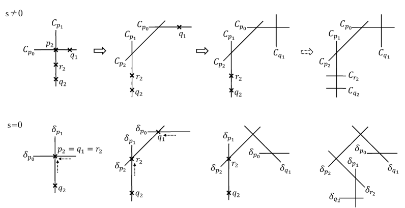
Figure 1: Exceptional curves and singularities of $SO(12)\rightarrow E_{7}$ : $p_{0}\rightarrow p_{1}\rightarrow p_{2}$ case.

3.1.3 Intersection diagram at $s=0$ : Transmutation of a root into a weight

In this subsection, we examine how $D_{6}$ Dynkin diagram at $s\neq 0$ becomes $A_{6}$ at $s=0$; in other words, how the sets $\{{\cal C}_{I}\}$ and $\{\delta_{I}\}$ are related. For this, as discovered in MT , it is important to know the $s\to 0$ limit of ${\cal C}$, which we write $\lim_{s\to 0}{\cal C}$. Here, we give a detailed explanation how this limit is explicitly calculated. It is worth noting that $\lim_{s\to 0}{\cal C}$ does not necessarily coincide with $\delta$. Suppose ${\cal C}$ and $\delta$ are defined in chart $A$, while ${\cal C}^{\prime}$ and $\delta^{\prime}$ are defined in a “deeper” chart $A^{\prime}$. By definition, $\lim_{s\to 0}{\cal C}=\delta$ in chart $A$. However, after ${\cal C}$ and $\delta$ are lifted up in chart $A^{\prime}$, ${\cal C}$ coexists with $\delta^{\prime}$ and hence $\lim_{s\to 0}{\cal C}$ may contain $\delta^{\prime}$. This can happen only after the lift-up. That is, lifting up and taking $s\to 0$ limit do not commute in general, and we should take $s\to 0$ after the lift-up.

Since the lift-ups have been completed in the previous subsection, all that is left is letting $s\to 0$. Suppose the limit is taken in a chart. As seen in the previous subsection, some of the lift-ups of ${\cal C}$’s and/or $\delta$’s may be invisible; that is, the limit consists only of the components visible in that chart. Thus the limit should be taken in every chart and the final form of $\lim_{s\to 0}{\cal C}$ is obtained as their union.

In chart $1$ and chart $2$, we can see from (42), (43) and (45) that $\lim_{s\to 0}{\cal C}_{i}=\delta_{i}$ for $i=p_{0},p_{1}$. In chart $3$, we encounter the first nontrivial result. From (46), we find in chart $3_{zxx}$ as

$$\lim_{s\to 0}{\cal C}_{p_{0}}=\delta_{p_{0}},\quad\lim_{s\to 0}{\cal C}_{p_{2}}=\{\tilde{x}_{1}=0,\,y_{3}^{2}=0\}=2\delta_{p_{2}}.$$ (56)

${\cal C}_{p_{2}}$ has only one component for $s\neq 0$, but after $s\rightarrow 0$, it splits into two overlapping (multiplicity two) $\delta_{p_{2}}$’s. Similarly, from (48), we find in chart $3_{zxz}$ as

$$\lim_{s\to 0}{\cal C}_{p_{1}}=\delta_{p_{1}},\quad\lim_{s\to 0}{\cal C}_{p_{2}}=\{z_{2}=0,\,y_{3}^{2}=0\}=2\delta_{p_{2}}.$$ (57)

In chart $3_{zxy}$, $\lim_{s\to 0}{\cal C}_{p_{2}}$ is invisible.

Next we consider charts $4_{zxx*}$ arising from the blow-up of $q_{1}$. In chart $4_{zxxx}$, ${\cal C}_{p_{2}}$ is visible, but $\delta_{p_{2}}$ is invisible (see (50)). Nevertheless, $\lim_{s\to 0}{\cal C}_{p_{2}}$ does exist. Actually, one can see from (50) that

$$\lim_{s\to 0}{\cal C}_{p_{2}}=\delta_{q_{1}}.$$ (58)

Also, we find $\lim_{s\to 0}{\cal C}_{p_{0}}=\delta_{p_{0}}\,,\,\lim_{s\to 0}{\cal C}_{q_{1}}=\delta_{q_{1}}.$ One can show that the same results are obtained in chart $4_{zxxy}$ except that ${\cal C}_{p_{0}}$ is invisible. In chart $4_{zxxz}$, one can see from (54) that ${\cal C}_{p_{2}}$ splits into two components as follows:

$$\lim_{s\to 0}{\cal C}_{p_{2}} = \{x_{4}z_{3}=0,y_{4}^{2}=x_{4}\}$$ (59)

$$= \{x_{4}=0,y_{4}^{2}=0\}\cup\{z_{3}=0,y_{4}^{2}=x_{4}\}$$

$$= 2\delta_{p_{2}}+\delta_{q_{1}}.$$

Also, $\lim_{s\to 0}{\cal C}_{q_{1}}=\delta_{q_{1}}$ is satisfied.

In charts $4_{zxz*}$, which arise from the blow-up of $r_{2}$, one can show by repeating the same argument that

$$\lim_{s\to 0}{\cal C}_{p_{2}}=2\delta_{p_{2}}+\delta_{r_{2}}\quad(\mbox{chart $4_{zxzx}$}),$$

$$\lim_{s\to 0}{\cal C}_{p_{2}}=\delta_{r_{2}},\hskip 38.41139pt(\mbox{chart $4_{zxzy}$, $4_{zxzz}$}).$$ (60)

All the other curves satisfy $\lim_{s\to 0}{\cal C}_{i}=\delta_{i}$.

Finally, after blowing up $q_{2}$, charts $3_{zz*}$ contain ${\cal C}_{q_{2}}$ as well as the lift-ups of ${\cal C}_{p_{0}}$ and ${\cal C}_{p_{1}}$. A similar analysis shows that $\lim_{s\to 0}{\cal C}_{i}=\delta_{i}$ for $i=p_{0},p_{1}$ and $q_{2}$.

Collecting all the above results, we find only ${\cal C}_{p_{2}}$ has a non-trivial limit. The final form of $\lim_{s\to 0}{\cal C}_{p_{2}}$ is given by the union of the components that are visible in each chart, and hence from (56), (57), (58), (59) and (60),

$$\lim_{s\to 0}{\cal C}_{p_{2}}=2\delta_{p_{2}}+\delta_{q_{1}}+\delta_{r_{2}}.$$ (61)

In conclusion, we find (Hereafter, $\lim_{s\to 0}$ will be omitted.)

$${\cal C}_{p_{0}}= \delta_{p_{0}},$$ (62)

$${\cal C}_{p_{1}}= \delta_{p_{1}},$$

$${\cal C}_{p_{2}}= 2\delta_{p_{2}}+\delta_{q_{1}}+\delta_{r_{2}},$$

$${\cal C}_{q_{1}}= \delta_{q_{1}},$$

$${\cal C}_{r_{2}}= \delta_{r_{2}},$$

$${\cal C}_{q_{2}}= \delta_{q_{2}}.$$

The intersection matrix of ${\cal C}$’s is the minus of the $D_{6}=SO(12)$ Cartan matrix:

$$-{\cal C}_{I}\cdot{\cal C}_{J} = \left(\begin{array}[]{cccccc}2&-1&0&0&0&0\\ -1&2&-1&0&0&0\\ 0&-1&2&-1&0&0\\ 0&0&-1&2&-1&-1\\ 0&0&0&-1&2&0\\ 0&0&0&-1&0&2\end{array}\right),$$ (69)

where $I,J=q_{1},p_{0},p_{2},p_{1},r_{2},q_{2}$ in this order. Note that this is different from the order of the blow-ups (see the upper rightmost diagram in Figure 1, or equivalently, the upper diagram in Figure 2 below). From (62), $\delta$’s are expressed in terms of ${\cal C}$’s. Then one can compute the intersection matrix of $\delta$’s, which is found to be

$$-\delta_{I}\cdot\delta_{J} = \left(\begin{array}[]{cccccc}2&-1&-1&0&0&0\\ -1&2&0&0&0&0\\ -1&0&\frac{3}{2}&0&-1&0\\ 0&0&0&2&-1&-1\\ 0&0&-1&-1&2&0\\ 0&0&0&-1&0&2\end{array}\right).$$ (76)

This is the minus of the $A_{6}=SU(7)$ Cartan matrix, except that the self-intersection number of $\delta_{p_{2}}$ is not $-2$, but $-\frac{3}{2}$. Namely, it is true that the intersection pattern of $\delta$’s is given by the $A_{6}$ Dynkin diagram, but their intersection “numbers” are slightly different from the corresponding $A_{6}$ Cartan matrix. This difference is expressed in the lower diagram in Figure 2 as the triangular (not circular) node. In summary,

$$\mbox{intersection pattern \, $\Rightarrow$ $A_{6}$ Dynkin diagram},$$

$$\mbox{intersection numbers $\Rightarrow$ $A_{6}$ Dynkin diagram with a triangular node}.$$ (77)

Let us call the latter diagram “intersection diagram”. Since it contains a $-\frac{3}{2}$ node, it is not a usual $A_{6}$ Dynkin diagram. In this sense, we conclude in the present case that the intersection diagram is an $A_{6}$ “non-Dynkin” diagram.

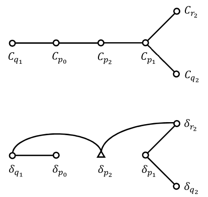
Figure 2: Generic $SO(12)$ intersection diagram at $s\neq 0$ (upper) and incomplete intersection diagram at $s=0$ (lower) of $SO(12)\rightarrow E_{7}$ : $p_{1}$-first ($p_{0}\rightarrow p_{1}\rightarrow p_{2}$) case.

In terms of ${\cal C}$’s, $\delta_{p_{2}}$ is written as $\delta_{p_{2}}=\frac{1}{2}({\cal C}_{p_{2}}-{\cal C}_{q_{1}}-{\cal C}_{r_{2}})$. This is one of the weights in the spinor representation of $SO(12)$. Thus we see that at a generic $s\neq 0$ codimension-one locus of the singularity the exceptional fibers after the resolutions form a root system of $SO(12)$, but at $s=0$ one of the simple roots (${\cal C}_{p_{2}}$) is transmuted to a weight in the spinor representation ($\delta_{p_{2}}$).

These $\delta$’s form a basis of the two-cycles appearing at the codimension-two singularity after the resolution. Let us consider the lattice spanned by $\delta$’s :

$$J=\sum_{I=q_{1},p_{0},p_{2},p_{1},r_{2},q_{2}}n_{I}\delta_{I}\quad(n_{I}\in{\boldmath Z}),$$ (78)

where each lattice point expresses a two-cycle at $s=0$. One can show by using (76) that

$$\sharp\,(J\cdot J=-2\,)\,\,\,=60,$$

$$\sharp\,\Big{(}J\cdot J=-\frac{3}{2}\,\Big{)}=32.$$ (79)

They respectively correspond to the adjoint representation (except the Cartan part) of $SO(12)$ and the spinor representation ${\bf 32}$ of $SO(12)$. The latter representation consists of 16 states with $n_{I}\geq 0$ for all $I$ and 16 states with $n_{I}\leq 0$ for all $I$. Note that, unlike in the cases of the ordinary (the complete) resolutions (1), there appears only one irreducible representation ($={\bf 32}$) in the integer span of the two-cycles at the singularity, indicating that it is a half-hypermultiplet.

3.2 Complete resolution: Blowing up $p_{1}$ first

3.2.1 Blowing up process

The geometry of complete resolution is given by setting $H_{n-r+4}=s^{2}$ instead of $H_{n-r+4}=s$ in (15) and (16) (the other polynomials are unchanged), we have

$$\Phi(x,y,z,s) = -y^{2}+x^{3}+f(z,s)x+g(z,s)=0,$$ (80)

where

$$f(z,s) = -3s^{4}z^{2}+z^{3},$$

$$g(z,s) = 2s^{6}z^{3}-s^{2}z^{4}.$$ (81)

Singularities can be blown up in the same way as in section 3.1.1. As a result, a new isolated (codimension-two) singularity $p_{3}$ arises in chart 3 after $p_{2}$ is blown up in chart $2_{zx}$. Regarding the structure of singularities, this is the only difference between complete and incomplete cases (see Table 2 below).

Table 2: $SO(12)\rightarrow E_{7}$: Complete case when $p_{1}$ is blown up first ($p_{0}\to p_{1}\to p_{2}$). The new isolated codimension-two conifold singularity is shown in red.

	1st blow up	2nd blow up	3rd blow up	4th blow up
\normalsize{$p_0$}⃝$\rightarrow$	\normalsize{$p_1(s^2:0:1)$}⃝$\rightarrow$	\normalsize{$p_2(1:0:0)$}⃝ $\mbox{(in $2_{zx}$)}\rightarrow$	\normalsize{$p_3(1:0:0;s=0)$}⃝$\mbox{(codim.2)}\rightarrow$	regular
	$q_{1}(-2s^{2}:0:1)$	$q_{1}(1:0:0)(\tilde{x}_{1}=-3s^{2})$	\normalsize{$q_1(1:0:0)(\tildex_1=-3s^2)$}⃝$\rightarrow$	regular
		$r_{2}(1:0:-3s^{2})$	\normalsize{$r_2(0:0:1)(z_2=-3s^2)$}⃝$\rightarrow$	regular
		\normalsize{$q_2(0:0:1)$}⃝ $\mbox{(in $2_{zz}$)}\rightarrow$	regular

Explicitly, the 3rd blow up (32) and (33) are replaced as follows:

3rd blow up

Chart $3_{zxx}$

$$\Psi_{zx}(\tilde{x}_{1},\tilde{x}_{1}y_{3},\tilde{x}_{1}z_{3},s) = \tilde{x}_{1}^{2}\Psi_{zxx}(\tilde{x}_{1},y_{3},z_{3},s),$$

$$\Psi_{zxx}(\tilde{x}_{1},y_{3},z_{3},s) = z_{3}(3s^{2}+\tilde{x}_{1}z_{3}+\tilde{x}_{1})-y_{3}^{2}.$$

$$\cal C {}_{p_{2}} 3_{zxx} : \tilde{x}_{1}=0,~{}~{}y_{3}^{2}=3s^{2}z_{3}.$$ in

Singularities $$: (\tilde{x}_{1},y_{3},z_{3},s)=(-3s^{2},0,0,s)(=q_{1}),(0,0,-1,0)(=p_{3}).$$ (82)

Chart $3_{zxy}$  Regular.

Chart $3_{zxz}$

$$\Psi_{zx}(x_{3}z_{2},y_{3}z_{2},z_{2},s) = z_{2}^{2}\Psi_{zxz}(x_{3},y_{3},z_{2},s),$$

$$\Psi_{zxz}(x_{3},y_{3},z_{2},s) = 3s^{2}x_{3}+x_{3}(x_{3}+1)z_{2}-y_{3}^{2}.$$

$$\cal C {}_{p_{2}} 3_{zxz} : z_{2}=0,~{}~{}y_{3}^{2}=3s^{2}x_{3}.$$ in

Singularities $$: (x_{3},y_{3},z_{2},s)=(0,0,-3s^{2},s)(=r_{2}),(-1,0,0,0)(=p_{3}).$$ (83)

The new isolated singularity $p_{3}$ is the conifold singularity. To see this, consider chart $3_{zxx}$ (82) and shift $p_{3}$ to the origin via

$$\tilde{z}_{3}\equiv z_{3}+1.$$ (84)

The defining equation then reads

$$\Upsilon_{zxx}(\tilde{x}_{1},y_{3},\tilde{z}_{3},s)\equiv\Psi_{zxx}(\tilde{x}_{1},y_{3},\tilde{z}_{3}-1,s).$$ (85)

The explicit form is

$$\Upsilon_{zxx}(\tilde{x}_{1},y_{3},\tilde{z}_{3},s)=-y_{3}^{2}+(-1+\tilde{z}_{3})(\tilde{x}_{1}\tilde{z}_{3}+3s^{2}),$$ (86)

where $p_{3}$ is located at $(\tilde{x}_{1},y_{3},\tilde{z}_{3},s)=(0,0,0,0)$. The leading terms of $\Upsilon_{zxx}$ can be written as $\Upsilon_{zxx}\sim\tilde{z}_{3}(-\tilde{x}_{1})-(y_{3}+i\sqrt{3}s)(y_{3}-i\sqrt{3}s)\sim X_{1}X_{4}-X_{2}X_{3},$ and hence $\Upsilon_{zxx}=0$ is a conifold. Including the subleading terms, we have

$$\Upsilon_{zxx}(\tilde{x}_{1},y_{3},\tilde{z}_{3},s) = \tilde{z}_{3}(-\tilde{x}_{1}+\tilde{x}_{1}\tilde{z}_{3}+3s^{2})-(y_{3}+i\sqrt{3}s)(y_{3}-i\sqrt{3}s)$$ (87)

$$= X_{1}X_{4}-X_{2}X_{3},$$

where $X_{i}$ are given by 

$$X_{1} = \tilde{z}_{3},$$

$$X_{4} = -\tilde{x}_{1}+\tilde{x}_{1}\tilde{z}_{3}+3s^{2},$$

$$X_{2} = y_{3}+i\sqrt{3}s,$$

$$X_{3} = y_{3}-i\sqrt{3}s.$$ (88)

$p_{3}$ is located at the origin $(X_{1},X_{2},X_{3},X_{4})=(0,0,0,0)$, which is the conifold singularity.

The exceptional curves existing in chart $3_{zxx}$ are given by replacing $s$ to $s^{2}$ in (46). After the coordinate changes (84) and (88), their positions read

Chart $3_{zxx}$

$${\cal C}_{p_{2}}:X_{4}=-3s^{2},\,\frac{(X_{2}+X_{3})^{2}}{4}=3s^{2}(X_{1}-1)\hskip 2.84544pt,\,\,\delta_{p_{2}}:X_{4}=0,\,X_{2}=X_{3}=0,$$

$${\cal C}_{p_{1}}:\mbox{Invisible}\,\hskip 147.95424pt,\,\,\delta_{p_{1}}:\mbox{Invisible},$$

$${\cal C}_{p_{0}}:X_{1}=1,\,X_{2}+X_{3}=0\hskip 88.2037pt,\,\,\delta_{p_{0}}:X_{1}=1,\,X_{2}=X_{3}=0,$$ (89)

where $s=-\frac{i}{2\sqrt{3}}(X_{2}-X_{3})$. The conifold singularity $p_{3}$ is contained in $\delta_{p_{2}}$, but not in $\delta_{p_{0}}$. Similarly, in chart $3_{zxz}$, $p_{3}$ is on $\delta_{p_{2}}$, but not on $\delta_{p_{1}}$. As for Figure 1, one new point $p_{3}$ is added on $\delta_{p_{2}}$ in the second figure of the bottom line.

3.2.2 Intersection diagram at $s=0$

Since $p_{3}$ is a codimension-two singularity, it does not change the intersection diagram for generic $s\neq 0$ (ordinary $SO(12)$ Dynkin diagram in Figure 2). Here we examine how the intersection diagram at $s=0$ is modified via the resolution of $p_{3}$.

The conifold singularity $p_{3}$ is resolved by inserting an exceptional curve $\hbox{\mybbsmall P}^{1}$ at the origin. This process is called the small resolution. We write the inserted $\hbox{\mybbsmall P}^{1}$ as $\delta_{\mbox{\scriptsize complete}}$. Since $p_{3}$ is contained only in $\delta_{p_{2}}$, $\delta_{\mbox{\scriptsize complete}}$ intersects only with $\delta_{p_{2}}$. Adding this node to Figure 2, we find that the intersection pattern becomes $E_{7}$ (see Figure 3 below). At this stage, however, it is not clear what intersection matrix is associated with this diagram. To clarify it, we need a lift-up.

The smooth geometry after the small resolution is covered by two local coordinate patches $H_{+}$ and $H_{-}$ (see Appendix C). By lifting up the relevant objects from chart $3$ into these patches, one can examine how the limit $s\to 0$ is modified from the incomplete case and what intersection matrix is obtained. Since $p_{3}$ is separated from $\delta_{p_{0}}$ and $\delta_{p_{1}}$, lifting up ${\cal C}_{p_{2}}$ and $\delta_{p_{2}}$ is sufficient. We consider chart $3_{zxx}$ (89).

The local coordinates of $H_{+}$ are $(X^{\prime}_{2},X^{\prime}_{4},\lambda)$ and the resolved geometry is obtained by the replacement (243):

$$(X_{1},X_{2},X_{3},X_{4})=(-\lambda X^{\prime}_{2},X^{\prime}_{2},-\lambda X^{\prime}_{4},X^{\prime}_{4}).$$ (90)

Here we put ^′ for the coordinates after the small resolution. The explicit form of $\delta_{\mbox{\scriptsize complete}}$ in chart $H_{+}$ is given by (244). The lift-ups of ${\cal C}_{p_{2}}$ and $\delta_{p_{2}}$ are given by substituting (90) into (89). Then we have

$\underline{\mbox{Chart $H_{+}$}}$

$$\hskip 213.39566pt\,\delta_{\mbox{\scriptsize complete}}:(X^{\prime}_{2},X^{\prime}_{4},\lambda)=(0,0,\lambda),$$

$${\cal C}_{p_{2}}:X^{\prime}_{4}=-3s^{2},\frac{(X^{\prime}_{2}-\lambda X^{\prime}_{4})^{2}}{4}=3s^{2}(-\lambda X^{\prime}_{2}-1)\hskip 2.84544pt,\,\delta_{p_{2}}:\mbox{Invisible},$$ (91)

where

$$s=-\frac{i}{2\sqrt{3}}(X^{\prime}_{2}+\lambda X^{\prime}_{4}).$$ (92)

$\delta_{p_{2}}$ is invisible, since $\delta_{p_{2}}$ (89) is given by $(-\lambda X^{\prime}_{2},X^{\prime}_{2},-\lambda X^{\prime}_{4},X^{\prime}_{4})=(X_{1},0,0,0)$ with $X_{1}\neq 0$, which is impossible. In this patch, $\delta_{p_{2}}$ and $\delta_{\mbox{\scriptsize complete}}$ do not intersect. The $s\to 0$ limit is given by the replacement $X^{\prime}_{2}=-\lambda X^{\prime}_{4}$, and hence

$$\lim_{s\to 0}{\cal C}_{p_{2}} = \{X^{\prime}_{4}=0,\lambda^{2}X^{\prime 2}_{4}=0\}\quad\mbox{with $X^{\prime}_{2}=-\lambda X^{\prime}_{4}$}$$ (93)

$$= \{(X^{\prime}_{2},X^{\prime}_{4},\lambda)=(0,0,\lambda)\}$$

$$= \delta_{\mbox{\scriptsize complete}}.$$

In the other patch $H_{-}$, the local coordinates are $(X^{\prime}_{1},X^{\prime}_{3},\mu)$ and the resolution is given by (246):

$$(X_{1},X_{2},X_{3},X_{4})=(X^{\prime}_{1},-\mu X^{\prime}_{1},X^{\prime}_{3},-\mu X^{\prime}_{3}).$$ (94)

In this patch, $\delta_{\mbox{\scriptsize complete}}$ (247) as well as ${\cal C}_{p_{2}}$ and $\delta_{p_{2}}$ (89) take the following forms:

$\underline{\mbox{Chart $H_{-}$}}$

$$\hskip 210.55022pt\,\delta_{\mbox{\scriptsize complete}}:(X^{\prime}_{1},X^{\prime}_{3},\mu)=(0,0,\mu),$$

$${\cal C}_{p_{2}}:\mu X^{\prime}_{3}=3s^{2},\,\frac{(X^{\prime}_{3}-\mu X^{\prime}_{1})^{2}}{4}=3s^{2}(X^{\prime}_{1}-1)\hskip 2.84544pt,\,\delta_{p_{2}}:(X^{\prime}_{1},X^{\prime}_{3},\mu)=(X^{\prime}_{1},0,0),$$ (95)

where

$$s=\frac{i}{2\sqrt{3}}(X^{\prime}_{3}+\mu X^{\prime}_{1}).$$ (96)

This time, $\delta_{p_{2}}$ is visible. $\delta_{p_{2}}$ and $\delta_{\mbox{\scriptsize complete}}$ are intersecting at $(X^{\prime}_{1},X^{\prime}_{3},\mu)=(0,0,0)$:

$$\delta_{p_{2}}\cdot\delta_{\mbox{\scriptsize complete}}\neq 0.$$ (97)

The $s\to 0$ limit is given by the replacement $X^{\prime}_{3}=-\mu X^{\prime}_{1}$:

$$\lim_{s\to 0}{\cal C}_{p_{2}} = \{-\mu^{2}X^{\prime}_{1}=0,\mu^{2}X^{\prime 2}_{1}=0\}\quad\mbox{with $X^{\prime}_{3}=-\mu X^{\prime}_{1}$}$$ (98)

$$= \{X^{\prime}_{1}=0\}\cup\{\mu^{2}=0\}\quad\mbox{with $X^{\prime}_{3}=-\mu X^{\prime}_{1}$}$$

$$= \{(X^{\prime}_{1},X^{\prime}_{3},\mu)=(0,0,\mu)\}\cup\{(X^{\prime}_{1},X^{\prime}_{3},\mu)=(X^{\prime}_{1},0,0)\}^{\otimes 2}$$

$$= \delta_{\mbox{\scriptsize complete}}+2\,\delta_{p_{2}}.$$

In conclusion, for the complete resolution, the new exceptional curve $\delta_{\mbox{\scriptsize complete}}$ is contained in $\lim_{s\to 0}{\cal C}_{p_{2}}$ with multiplicity one, and (62) is modified as

$${\cal C}_{p_{0}}= \delta_{p_{0}},$$ (99)

$${\cal C}_{p_{1}}= \delta_{p_{1}},$$

$${\cal C}_{p_{2}}= 2\delta_{p_{2}}+\delta_{q_{1}}+\delta_{r_{2}}+\delta_{\mbox{\scriptsize complete}},$$

$${\cal C}_{q_{1}}= \delta_{q_{1}},$$

$${\cal C}_{r_{2}}= \delta_{r_{2}},$$

$${\cal C}_{q_{2}}= \delta_{q_{2}}.$$

Then, assuming that the intersection matrix of these seven $\delta$’s is just the minus of ordinary $E_{7}$ Cartan matrix, we find that the intersection matrix of the six ${\cal C}$’s computed by (99) is precisely the minus of the $SO(12)$ Cartan matrix. It means that, in contrast to the incomplete case, $\delta$’s have no node with self-intersection number $-\frac{3}{2}$ and the intersection diagram is the ordinary $E_{7}$ Dynkin diagram. That is, $\delta_{p_{2}}$, whose self-intersection number is $-\frac{3}{2}$ (triangular node) in the incomplete case, becomes the ordinary node with self-intersection $-2$ (circular node) by virtue of the existence of $\delta_{\mbox{\scriptsize complete}}$. The result is summarized in Figure 3. As usual, two cycles $J$ spanned by the seven $\delta$’s with $J\cdot J=-2$ contain two ${\bf 32}$’s as in (1).

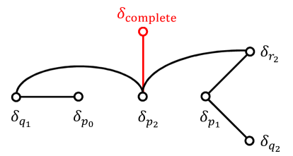
Figure 3: Complete $E_{7}$ intersection diagram of $SO(12)\rightarrow E_{7}$ : $p_{1}$-first ($p_{0}\rightarrow p_{1}\rightarrow p_{2}$) case.

3.3 Incomplete resolution: Blowing up $q_{1}$ first

3.3.1 Blowing up process

In section 3.1, between the two singularities $p_{1}$ and $q_{1}$ arising from the first blow up in chart $1_{z}$ (28), $p_{1}$ was blown up first. In this section, let us blow up $q_{1}$ first and see the differences. This time we make a shift of the coordinate $x_{1}$ so that $q_{1}$ comes to $(0,0,0,s)$: We define

$$\Sigma_{z}(\tilde{x}_{1},y_{1},z,s) \equiv \Phi_{z}(\tilde{x}_{1}-2s,y_{1},z,s).$$ (100)

$\Sigma_{z}(\tilde{x}_{1},y_{1},z,s)=0$ has singularities $(3s,0,0,s)$ $(=p_{1})$ and $(0,0,0,s)$ $(=q_{1})$. We blow up the latter singularity. The process is completely parallel to that in the previous section so we will only describe the relevant charts and show the main differences from the previous case. For later use, we also present the definition of $\delta$ and the lift-ups of ${\cal C}$ and $\delta$. For the $p_{1}$-first case studied in the previous sections, the exceptional curves arising from the blow-ups of the singularities $p_{0}$, $p_{1}$, $p_{2}$, $q_{1}$, $r_{2}$ and $q_{2}$ are respectively expressed by ${\cal C}_{p_{0}}$, ${\cal C}_{p_{1}}$, ${\cal C}_{p_{2}}$, ${\cal C}_{q_{1}}$, ${\cal C}_{r_{2}}$ and ${\cal C}_{q_{2}}$. We use the same notation for the $q_{1}$-first case as well.

2nd blow up

From the blow-up of $q_{1}$, ${\cal C}_{q_{1}}$ arises. ${\cal C}_{p_{0}}$ and $\delta_{p_{0}}$ are lifted up from chart $1_{z}$. Chart $2_{zx}$

$$\Sigma_{z}(\tilde{x}_{1},\tilde{x}_{1}y_{2},\tilde{x}_{1}z_{2},s) = \tilde{x}_{1}^{2}\Sigma_{zx}(\tilde{x}_{1},y_{2},z_{2},s),$$

$$\Sigma_{zx}(\tilde{x}_{1},y_{2},z_{2},s) = z_{2}(3s-\tilde{x}_{1})(3s-\tilde{x}_{1}-z_{2})-y_{2}^{2}.$$

$$\cal C {}_{q_{1}} : \tilde{x}_{1}=0,~{}~{}3sz_{2}(3s-z_{2})-y_{2}^{2}=0,\quad\delta_{q_{1}}\,:\,\tilde{x}_{1}=0,~{}y_{2}=0,$$

$$\cal C {}_{p_{0}} : z_{2}=0,~{}~{}y_{2}=0\hskip 79.6678pt,\quad\delta_{p_{0}}\,:\,z_{2}=0,~{}y_{2}=0.$$

Singularities $$: (\tilde{x}_{1},y_{2},z_{2},s)=(3s,0,0,s)(=p_{1}).$$ (101)

The positions of these objects are depicted in the leftmost column of Figure 4. There are no other singularities in chart $2_{zy}$ or $2_{zz}$, so we blow up $p_{1}$ in chart $2_{zx}$. Again, we need to shift the coordinate so that the singularity we now blow up comes to the origin:

$$\Psi_{zx}(\!\tilde{\tilde{~{}x_{1}}},y_{2},z_{2},s) \equiv \Sigma_{zx}(\!\tilde{\tilde{~{}x_{1}}}+3s,y_{2},z_{2},s).$$ (102)

3rd blow up

The relevant charts are $3_{zxx}$ and $3_{zxz}$. From the blow-up of $p_{1}$, ${\cal C}_{p_{1}}$ arises.

Chart $3_{zxx}$

$$\Psi_{zx}(\!\tilde{\tilde{~{}x_{1}}},\!\tilde{\tilde{~{}x_{1}}}y_{3},\!\tilde{\tilde{~{}x_{1}}}z_{3},s) = \!\tilde{\tilde{~{}x_{1}}}^{2}\Psi_{zxx}(\!\tilde{\tilde{~{}x_{1}}},y_{3},z_{3},s),$$

$$\Psi_{zxx}(\!\tilde{\tilde{~{}x_{1}}},y_{3},z_{3},s) = \!\tilde{\tilde{~{}x_{1}}}z_{3}(z_{3}+1)-y_{3}^{2}.$$

$$\cal C {}_{p_{1}} : \!\tilde{\tilde{~{}x_{1}}}=0,~{}~{}y_{3}=0\hskip 91.04872pt,\quad\delta_{p_{1}}\,\,:\,\tilde{\tilde{~{}x_{1}}}=0,~{}y_{3}=0,$$

$$\cal C {}_{q_{1}} : \tilde{\tilde{~{}x_{1}}}=-3s,~{}~{}\tilde{\tilde{~{}x_{1}}}z_{3}(1+z_{3})-y_{3}^{2}=0,\quad\delta_{q_{1}}\,:\,\mbox{Invisible},$$

$$\cal C {}_{p_{0}} : z_{3}=0,~{}~{}y_{3}=0\hskip 93.89418pt,\quad\delta_{p_{0}}\,\,:\,z_{3}=0,~{}y_{3}=0.$$

Singularities $$: (\!\tilde{\tilde{~{}x_{1}}},y_{3},z_{3},s)=(0,0,-1,s)(=r_{2}),(0,0,0,s)(=p_{2}).$$ (103)

Chart $3_{zxz}$

$$\Psi_{zx}(x_{3}z_{2},y_{3}z_{2},z_{2},s) = z_{2}^{2}\Psi_{zxz}(x_{3},y_{3},z_{2},s),$$

$$\Psi_{zxx}(x_{3},y_{3},z_{2},s) = x_{3}(x_{3}+1)z_{2}-y_{3}^{2}.$$

$$\cal C {}_{p_{1}} : z_{2}=0,~{}~{}y_{3}=0\hskip 96.73918pt,\quad\delta_{p_{1}}\,\,:\,z_{2}=0,~{}y_{3}=0,$$

$$\cal C {}_{q_{1}} : x_{3}z_{2}=-3s,~{}~{}x_{3}z_{2}(x_{3}+1)-y_{3}^{2}=0,\quad\delta_{q_{1}}\,:\,x_{3}=0,\,y_{3}=0,$$

$$\cal C {}_{p_{0}} : \mbox{Invisible}\hskip 130.88284pt,\quad\delta_{p_{0}}\,\,:\,\mbox{Invisible}.$$

Singularities $$: (x_{3},y_{3},z_{2},s)=(-1,0,0,s)(=r_{2}),(0,0,0,s)(=q_{2}).$$ (104)

Note that ${\cal C}_{q_{1}}$ and $\delta_{q_{1}}$ are independently lifted up from (101). The positions of these objects are depicted in the middle column of Figure 4. One can see from (103) and (104) that the remaining three singularities $p_{2}$, $r_{2}$ and $q_{2}$ are separated for all $s$ (not only for $s\neq 0$ but also for $s=0$), and hence they are independently blown up. The whole blowing up process is summarized in Table 3. The resulting intersection patterns are depicted in the rightmost column of Figure 4. For $s\neq 0$, the intersection pattern is the $D_{6}$ Dynkin diagram, which is identical to the one in the $p_{1}$-first case (see the upper rightmost diagram in Figure 1, or the upper diagram in Figure 2). The orders of the nodes are the same as well. On the other hand, the intersection pattern at $s=0$ is the $E_{6}$ Dynkin diagram, which is different from the one ($A_{6}$) in the $p_{1}$-first case.

Table 3: $SO(12)\rightarrow E_{7}$: Incomplete case when $q_{1}$ is blown up first ($p_{0}\to q_{1}$).

	1st blow up	2nd blow up	3rd blow up	4th blow up
\normalsize{$p_0$}⃝$\rightarrow$	\normalsize{$q_1(-2s:0:1)$}⃝$\rightarrow$	regular
	$p_{1}(s:0:1)$	\normalsize{$p_1(1:0:0)$}⃝$(\tilde{x}_{1}=3s)\rightarrow$	\normalsize{$p_2(1:0:0)$}⃝$\rightarrow$	regular
			\normalsize{$q_2(0:0:1)$}⃝$\rightarrow$	regular
			\normalsize{$r_2(1:0:-1)$}⃝$\rightarrow$	regular

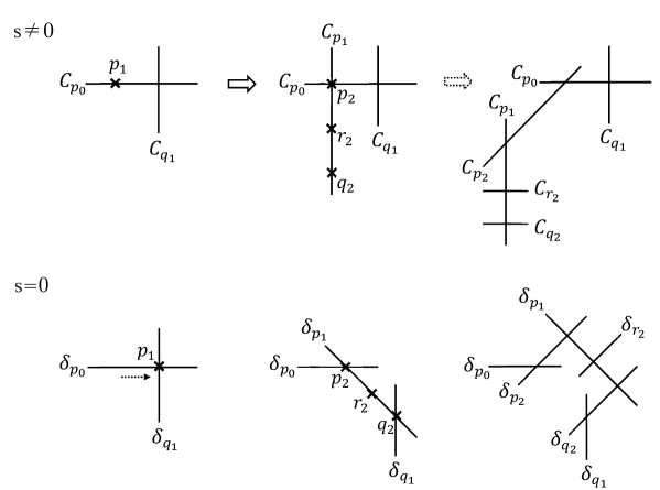
Figure 4: Exceptional curves and singularities of $SO(12)\rightarrow E_{7}$ : $p_{0}\rightarrow q_{1}$ case.

3.3.2 Intersection diagram at $s=0$: Differences from the $p_{1}$-first case

Following the same procedure given in section 3.1.3, we find the $s\to 0$ limit of ${\cal C}$ for the $q_{1}$-first case as

$${\cal C}_{p_{0}}= \delta_{p_{0}},$$ (105)

$${\cal C}_{q_{1}}= 2\delta_{q_{1}}+2\delta_{p_{1}}+\delta_{p_{2}}+2\delta_{q_{2}}+\delta_{r_{2}},$$

$${\cal C}_{p_{1}}= \delta_{p_{1}},$$

$${\cal C}_{p_{2}}= \delta_{p_{2}},$$

$${\cal C}_{r_{2}}= \delta_{r_{2}},$$

$${\cal C}_{q_{2}}= \delta_{q_{2}}.$$

The first two terms of ${\cal C}_{q_{1}}$ are readily observed in chart $3$ (see (103) and (104)). The other terms of ${\cal C}_{q_{1}}$ can only be seen in deeper charts. We skip the detail of the derivation.

The intersection matrix among ${\cal C}$’s is the same one with the $p_{1}$-first case and is given by (69) with the same order $I,J=q_{1},p_{0},p_{2},p_{1},r_{2},q_{2}$. Then (105) yields the intersection matrix of $\delta$’s as

$$-\delta_{I}\cdot\delta_{J} = \left(\begin{array}[]{cccccc}\frac{3}{2}&0&0&0&0&-1\\ 0&2&-1&0&0&0\\ 0&-1&2&-1&0&0\\ 0&0&-1&2&-1&-1\\ 0&0&0&-1&2&0\\ -1&0&0&-1&0&2\end{array}\right).$$ (112)

This is almost the $E_{6}$ Cartan matrix except that the self-intersection number of $\delta_{q_{1}}$ is $-\frac{3}{2}$, which is expressed as a triangular node in Figure 5. Thus the intersection diagram for this case is an $E_{6}$ non-Dynkin diagram.

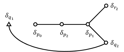
Figure 5: Incomplete intersection diagram of $SO(12)\rightarrow E_{7}$ : $q_{1}$-first ($p_{0}\rightarrow q_{1}$) case.

We can search for the elements of the form $\sum_{I=q_{1},p_{0},p_{2},p_{1},r_{2},q_{2}}n_{I}\delta_{I}$ whose square is $-\frac{3}{2}$ to find, again, that there are $16+16$ such elements, the former of which have $n_{I}\geq 0$ for all $I$, and the latter of which have $n_{I}\leq 0$ for all $I$. Thus, in this case as well, there is only one irreducible representation ($={\bf 32}$) at the singularity, showing that it is a half-hypermultiplet.

3.4 Complete resolutions: Blowing up $q_{1}$ first

The process of the blow-ups is almost the same as that in the incomplete resolutions. A difference arises in chart $2_{zz}$, where a conifold singularity is developed at $(x_{2},y_{2},z,s)=(0,0,0,0)$, which we denote by $q_{3}$ (shown in red in Table 4), where the relation to the coordinates in chart $1_{z}$ is $(\tilde{x}_{1},y_{1},z,s)=(x_{2}z,y_{2}z,z,s)$. This is an isolated codimension-two singularity developed only at $s=0$. Since this is in chart $2_{zz}$, this singularity is located at $(0:0:1)$ on $\hbox{\mybbsmall P}^{2}$ emerged by the blow up at $s=0$. Therefore, it is not visible in chart $2_{zx}$ or $3_{zx*}$. Moreover, after the coordinate shift similar to (100), $\Psi_{zx}$ becomes identical to the incomplete case. Thus the process is the same as the incomplete case afterwards. Therefore, the only extra exceptional curve is the one arising from the small resolution of the isolated conifold singularity on $\delta_{q_{1}}$. This adds an extra node to the diagram in the Figure 5, as we show in Figure 6. We denote this new curve as $\delta_{\rm complete}$ here. This is $E_{7}$, and the extra node again extends from $\delta_{q_{1}}$ that was the “weight” node represented by the triangle in the incomplete case. How $\delta_{\rm complete}$ modifies the $\lim_{s\to 0}{\cal C}$ can be seen in the same way as explained in section 3.2.2. The result is

$${\cal C}_{p_{0}}= \delta_{p_{0}},$$ (113)

$${\cal C}_{q_{1}}= 2\delta_{q_{1}}+2\delta_{p_{1}}+\delta_{p_{2}}+2\delta_{q_{2}}+\delta_{r_{2}}+\delta_{\rm complete},$$

$${\cal C}_{p_{1}}= \delta_{p_{1}},$$

$${\cal C}_{p_{2}}= \delta_{p_{2}},$$

$${\cal C}_{r_{2}}= \delta_{r_{2}},$$

$${\cal C}_{q_{2}}= \delta_{q_{2}}.$$

This reproduces the minus of the $D_{6}$ Cartan matrix as the intersection matrix of ${\cal C}$’s if the intersections among $\delta$’s are given by the minus of the proper $E_{7}$ Cartan matrix. Therefore, in the complete case, $\delta_{q_{1}}$ becomes an ordinary node with self-intersection $-2$ as shown in Figure 6.

Table 4: $SO(12)\rightarrow E_{7}$: Complete case when $q_{1}$ is blown up first ($p_{0}\to q_{1}$).

	1st blow up	2nd blow up	3rd blow up	4th blow up
\normalsize{$p_0$}⃝$\rightarrow$	\normalsize{$q_1(-2s:0:1)$}⃝$\rightarrow$	\normalsize{$q_3(0:0:1;s=0)$}⃝$\mbox{(codim.2)}\rightarrow$	regular
	$p_{1}(s:0:1)$	\normalsize{$p_1(1:0:0)$}⃝$(\tilde{x}_{1}=3s)\rightarrow$	\normalsize{$p_2(1:0:0)$}⃝$\rightarrow$	regular
			\normalsize{$q_2(0:0:1)$}⃝$\rightarrow$	regular
			\normalsize{$r_2(1:0:-1)$}⃝$\rightarrow$	regular

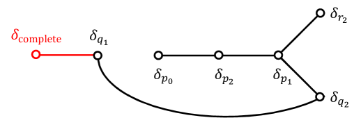
Figure 6: Complete $E_{7}$ intersection diagram of $SO(12)\rightarrow E_{7}$ : $q_{1}$-first ($p_{0}\rightarrow q_{1}$) case.

3.5 Other inequivalent orderings

So far we have considered incomplete and complete resolutions where the order of blowing up singularities is $p_{0}\rightarrow p_{1}\rightarrow p_{2}$ and $p_{0}\rightarrow q_{1}$. In the former case, we have also two codimension-one singularities $q_{1}$ and $r_{2}$, besides $p_{2}$ and $q_{2}$, after the 2nd blow up, as shown in Table 1. Since $q_{2}$ never coincides with the other three for any value of $s$, it can be blown up independently at any stage. On the other hand, $p_{2}$, $q_{1}$ and $r_{2}$ become the same point $(1:0:0)$ on the $\hbox{\mybbsmall P}^{2}$ at $s=0$, so a different intersection diagram arises if we blow up $q_{1}$ or $r_{2}$ instead of $p_{2}$ after blowing up $p_{1}$. The concrete process is similar to the previous cases so we only describe the results.

$p_{0}\rightarrow p_{1}\rightarrow q_{1}$ case

If $q_{1}$ is blown up after $p_{1}$, the relations among ${\cal C}$’s and $\delta$’s are given by (the modifications via $\delta_{\scriptsize\mbox{complete}}$ in the complete case are shown in the parentheses)

$${\cal C}_{p_{0}}= \delta_{p_{0}},$$ (114)

$${\cal C}_{p_{1}}= \delta_{p_{1}}+\delta_{q_{1}}\,(+\delta_{\scriptsize\mbox{complete}}),$$

$${\cal C}_{q_{1}}= 2\delta_{q_{1}}+\delta_{p_{2}}+\delta_{r_{2}}\,(+\delta_{\scriptsize\mbox{complete}}),$$

$${\cal C}_{p_{2}}= \delta_{p_{2}},$$

$${\cal C}_{r_{2}}= \delta_{r_{2}},$$

$${\cal C}_{q_{2}}= \delta_{q_{2}}.$$

The intersection matrix of ${\cal C}$’s is the same one as before. The intersection diagrams of $\delta$’s for incomplete / complete cases are shown in Figure 7. The diagram for the incomplete case is an $E_{6}$ non-Dynkin diagram, which is similar to the $p_{0}\rightarrow q_{1}$ case. But this time there are two $-\frac{3}{2}$ nodes. The intersection matrix is given by

$$-\delta_{I}\cdot\delta_{J} = \left(\begin{array}[]{cccccc}\frac{3}{2}&0&-1&-\frac{1}{2}&-1&0\\ 0&2&-1&0&0&0\\ -1&-1&2&0&0&0\\ -\frac{1}{2}&0&0&\frac{3}{2}&0&-1\\ -1&0&0&0&2&0\\ 0&0&0&-1&0&2\end{array}\right),$$ (121)

with the same order $I,J=q_{1},p_{0},p_{2},p_{1},r_{2},q_{2}$ as before. Note that the intersection of the two $-\frac{3}{2}$ nodes is $\frac{1}{2}$.

Again, there is only one ${\bf 32}$ at $s=0$ as two-cycles $J$ (78) satisfying $J\cdot J=-\frac{3}{2}$. For the complete case, $\delta_{\scriptsize\mbox{complete}}$ bridges the two $-\frac{3}{2}$ nodes and forms the ordinary $E_{7}$ intersection diagram.

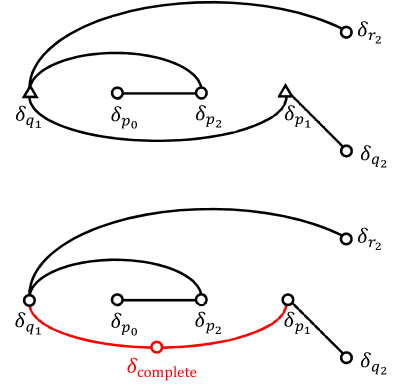
Figure 7: Incomplete/complete intersection diagrams of $SO(12)\rightarrow E_{7}$ : $p_{1}$-first ($p_{0}\rightarrow p_{1}\rightarrow q_{1}$) case.

$p_{0}\rightarrow p_{1}\rightarrow r_{2}$ case

If $r_{2}$ is blown up after $p_{1}$, the relations among ${\cal C}$’s and $\delta$’s are found to be

$${\cal C}_{p_{0}}= \delta_{p_{0}}+\delta_{r_{2}}\,(+\delta_{\scriptsize\mbox{complete}}),$$ (122)

$${\cal C}_{p_{1}}= \delta_{p_{1}},$$

$${\cal C}_{r_{2}}= 2\delta_{r_{2}}+\delta_{p_{2}}+\delta_{q_{1}}\,(+\delta_{\scriptsize\mbox{complete}}),$$

$${\cal C}_{q_{1}}= \delta_{q_{1}},$$

$${\cal C}_{p_{2}}= \delta_{p_{2}},$$

$${\cal C}_{q_{2}}= \delta_{q_{2}},$$

and the intersection diagrams of $\delta$’s are as shown in Figure 8. This time, the diagram for the incomplete case is a $D_{6}$ non-Dynkin diagram. There are two nodes with self intersections $-\frac{3}{2}$ and their mutual intersection is $\frac{1}{2}$. As before, only one ${\bf 32}$ appears at $s=0$ as $J\cdot J=-\frac{3}{2}$ states. For the complete case, $\delta_{\scriptsize\mbox{complete}}$ bridges the two $-\frac{3}{2}$ nodes and forms the ordinary $E_{7}$ intersection diagram.

This exhausts all the possibilities of changing the order of the singularities we blow up.

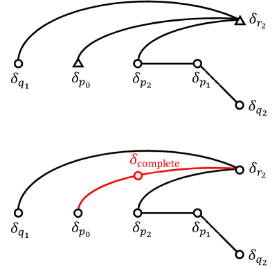
Figure 8: Incomplete/complete intersection diagrams of $SO(12)\rightarrow E_{7}$ : $p_{1}$-first ($p_{0}\rightarrow p_{1}\rightarrow r_{2}$) case.

3.6 Comparison with the results of the M-theory Coulomb branch analysis

In the previous sections we have obtained four distinct incomplete intersection diagrams of the fibers at the codimension-two singularity. Let us compare our results with those obtained by the M-theory Coulomb branch analysis BoxGraphs .

In general, F-theory compactifications on Calabi-Yau four-folds are dual to M-theory compactifications on Calabi-Yau four-folds, which present three-dimensional ${\cal N}=2$ supersymmetric gauge theories. The geometry of the Calabi-Yau four-fold determines the structure of the gauge theory. In particular, the codimension-one singularity decides the gauge group, and the network of the resolution corresponds to the structure of the classical Coulomb phase since the resolution corresponds to the symmetry breaking.

We consider three-dimensional gauge theory with a gauge group $G$ and with $N_{f}$ chiral multiplets in a representation ${\bf R}_{f}$. We set the masses of the chiral multiplets to zero. In addition, we assume that there is no classical Chern-Simons term. The vector multiplet in the adjoint representation includes a real scalar field $\phi$. In general, the gauge group $G$ breaks to $U(1)^{r}$ by the VEVs of the scalar, where $r={\rm rank}(G)$. We choose the fundamental Weyl chamber as

$$\vec{\alpha}_{i}\cdot\vec{\phi}>0,$$ (123)

where $\vec{\alpha}_{i}\ (i=1,2,\ldots,r)$ are the simple roots of $G$. $\vec{\phi}=(\phi^{1},\phi^{2},\ldots,\phi^{r})$ are the VEVs in the Cartan subalgebra of $G$.

Now we have the chiral multiplets, which make a substructure in the Coulomb branch. The Lagrangian includes the mass terms of the chiral multiplets $Q^{(f)}$:

$${\cal L}_{\rm mass}=\sum_{f}\left|\phi Q^{(f)}\right|^{2}=\sum_{f}\left|\vec{\phi}\cdot\vec{\omega}_{f}\right|^{2}\left|Q^{(f)}\right|^{2},$$ (124)

where $\vec{\omega}_{f}$ are weights of ${\bf R}_{f}$ representation. Note that when $\vec{\phi}\cdot\vec{\omega}_{f}=0$, the corresponding matter becomes massless.

We can classify the regions of the Coulomb branch. A region is bounded by the zero loci of $\vec{\phi}\cdot\vec{\omega}_{f}$, namely, it is characterized by $\vec{\phi}\cdot\vec{\omega}_{f}>0$ or $\vec{\phi}\cdot\vec{\omega}_{f}<0$. However, not all regions are allowed since we are working on the fundamental Weyl chamber (123). The allowed regions of the Coulomb branch are completely classified by the decorated box graphs defined by a collection of boxes with signs (or colors) BoxGraphs .

Although the analysis of BoxGraphs is based on the Coulomb branch of the three-dimensional M-theory, which basically applies to a resolution of a Calabi-Yau four-fold such as EsoleYau ; MarsanoSSNameki ; EsoleShaoYau ; BraunNameki , it is interesting to compare our results with the corresponding box graphs obtained in BoxGraphs since the scalars of the five-dimensional M-theory, which are supposed to describe the resolution of a Calabi-Yau three-fold, partly comprise the three-dimensional scalars.

In BoxGraphs , the intersection diagrams for the singularity enhancement $SO(12)\rightarrow E_{7}$ are given in Figure 33 of that paper. We can see that the intersection diagrams for incomplete resolutions shown in Figures 5, 7 and 8 of the present paper are the ones at the bottom, the third from the bottom and the second from the top of the left column of Figure 33 of BoxGraphs . Also, the (lower) diagram in Figure 2 of this paper is the diagram in the right column of Figure 33 of BoxGraphs . Thus, all the four intersection diagrams we found here have corresponding box graphs obtained in BoxGraphs describing different phases of the three-dimensional gauge theory. Note that any two of them are not adjacent to each other in the seven graphs of Figure 33 of BoxGraphs . This is consistent, as the two adjacent graphs of BoxGraphs are related by a flop, and the change of the order of the singularities is not a flop. Indeed, we do not have any conifold singularities until we consider a complete resolution. This is one of the differences between the resolutions in six and four dimensions.

4 $E_{7}\rightarrow E_{8}$

4.1 Incomplete resolution: Blowing up $p_{2}$ first

4.1.1 Blowing up process

In this case we take $f_{n+8}=s$ with setting $g_{n+12}=1$, $f_{8}=g_{12}=0$ in (19) and (20) :

$$f(z,s) = sz^{3},$$

$$g(z,s) = z^{5}.$$ (125)

At $s\neq 0$, the orders of $f$, $g$ and $\Delta$ in $z$ are $(3,5,9)$, while at $s=0$, they satisfy $(\geq 4,5,10)$. Hence it describes the enhancement $III^{*}\rightarrow II^{*}$ ($E_{7}\rightarrow E_{8}$) of the Kodaira type.

$\Phi(x,y,z,s)=0$ has a codimension-one singularity at $p_{0}=(0,0,0,s)$. The concrete process of the incomplete resolution goes as follows (an exceptional curve arising from blowing up a singularity $p$ will be denoted by ${\cal C}_{p}$):

1st blow up

Chart $1_{x}$

$$\Phi(x,xy_{1},xz_{1},s) = x^{2}\Phi_{x}(x,y_{1},z_{1},s),$$

$$\Phi_{x}(x,y_{1},z_{1},s) = sx^{2}z_{1}^{3}+x^{3}z_{1}^{5}+x-y_{1}^{2}.$$

$$\cal C {}_{p_{0}} 1_{x} : x=0,~{}~{}y_{1}=0.$$ in

Singularities $$:$$ None (126)

Chart $1_{y}$  $\cal C$${}_{p_{0}}$ is not visible in this chart.

Chart $1_{z}$

$$\Phi(x_{1}z,y_{1}z,z,s) = z^{2}\Phi_{z}(x_{1},y_{1},z,s),$$

$$\Phi_{z}(x_{1},y_{1},z,s) = z\left(x_{1}zs+x_{1}^{3}+z^{2}\right)-y_{1}^{2}.$$

$$\cal C {}_{p_{0}} 1_{z} : z=0,~{}~{}y_{1}=0.$$ in

Singularities $$: (x_{1},y_{1},z,s)=(0,0,0,s).$$ (127)

We refer to this singularity as $p_{1}$.

2nd blow up

Chart $2_{zx}$

$$\Phi_{z}(x_{1},x_{1}y_{2},x_{1}z_{2},s) = x_{1}^{2}\Phi_{zx}(x_{1},y_{2},z_{2},s),$$

$$\Phi_{zx}(x_{1},y_{2},z_{2},s) = z_{2}x_{1}\left(z_{2}(s+z_{2})+x_{1}\right)-y_{2}^{2}.$$

$$\cal C {}_{p_{1}} 2_{zx} : x_{1}=0,~{}~{}y_{2}=0.$$ in

Singularities $$: (x_{1},y_{2},z_{2},s)=(0,0,-s,s)(=q_{2}),(0,0,0,s)(=p_{2}).$$ (128)

Here we see two singularities on $\cal C$${}_{p_{1}}$ which coincide with each other at $s=0$.

Chart $2_{zy}$  $\cal C$${}_{p_{1}}$ is not visible in this chart.

Chart $2_{zz}$

$$\Phi_{z}(x_{2}z,y_{2}z,z,s) = z^{2}\Phi_{zz}(x_{2},y_{2},z,s),$$

$$\Phi_{zz}(x_{2},y_{2},z,s) = z\left(sx_{2}+zx_{2}^{3}+1\right)-y_{2}^{2}.$$

$$\cal C {}_{p_{1}} 2_{zz} : z=0,~{}~{}y_{2}=0.$$ in

Singularities $$: (x_{2},y_{2},z,s)=(-\frac{1}{s},0,0,s).$$ (129)

This singularity is $q_{2}$, which is also seen in chart $2_{zx}$. At this stage, we have two singularities $p_{2}$ and $q_{2}$. In this section we blow up $p_{2}$ first. We can see this singularity in chart $2_{zx}$ only, so we consider $\Phi_{zx}(x_{1},y_{2},z_{2},s)$ in the next blow up.

3rd blow up

Chart $3_{zxx}$

$$\Phi_{zx}(x_{1},x_{1}y_{3},x_{1}z_{3},s) = x_{1}^{2}\Phi_{zxx}(x_{1},y_{3},z_{3},s),$$

$$\Phi_{zxx}(x_{1},y_{3},z_{3},s) = z_{3}x_{1}\left(sz_{3}+z_{3}^{2}x_{1}+1\right)-y_{3}^{2}.$$

$$\cal C {}_{p_{2}} 3_{zxx} : x_{1}=0,~{}~{}y_{3}=0.$$ in

Singularities $$: (x_{1},y_{3},z_{3},s)=(0,0,-\frac{1}{s},s)(=r_{3}),(0,0,0,s)(=p_{3}).$$ (130)

We name the first singularity $r_{3}$, and the second singularity $p_{3}$.

Chart $3_{zxy}$  Regular.

Chart $3_{zxz}$

$$\Phi_{zx}(x_{3}z_{2},y_{3}z_{2},z_{2},s) = z_{2}^{2}\Phi_{zxz}(x_{3},y_{3},z_{2},s),$$

$$\Phi_{zxz}(x_{3},y_{3},z_{2},s) = z_{2}x_{3}\left(s+z_{2}+x_{3}\right)-y_{3}^{2}.$$

$$\cal C {}_{p_{2}} 3_{zxz} : z_{2}=0,~{}~{}y_{3}=0.$$ in

Singularities $$: (x_{3},y_{3},z_{2},s)=(0,0,-s,s)(=q_{2}),(0,0,0,s)(=q_{3}),$$ (131)

$$\hskip 73.97733pt(-s,0,0,s)(=r_{3}).$$

The first singularity is not on $\cal C$${}_{p_{2}}$ unless $s=0$; this is $q_{2}$. We name the second singularity $q_{3}$. The third one is $r_{3}$ already seen in chart $3_{zxx}$.

When $s\rightarrow 0$, the three singularities $q_{2}$, $q_{3}$ and $r_{3}$ in chart $3_{zxz}$ coincide with each other, and which one we blow up next affects the proceeding process. In this section, we consider the case $q_{3}$ is blown up next. On the other hand, $p_{3}$ in chart $3_{zxx}$ is separated from these points even when $s\rightarrow 0$ and can be blown up independently. We leave the blow-up of $p_{3}$ until later and work on the blow-up of $q_{3}$.

4th blow up at $q_{3}$

We next blow up $q_{3}$. Using $\Phi_{zxz}(x_{3},y_{3},z_{2},s)$, we find

Chart $4_{zxzx}$

$$\Phi_{zxz}(x_{3},x_{3}y_{4},x_{3}z_{4},s) = x_{3}^{2}\Phi_{zxzx}(x_{3},y_{4},z_{4},s),$$

$$\Phi_{zxzx}(x_{3},y_{4},z_{4},s) = z_{4}\left(s+z_{4}x_{3}+x_{3}\right)-y_{4}^{2}.$$

$$\cal C {}_{q_{3}} 4_{zxzx} : x_{3}=0,~{}~{}y_{4}^{2}=sz_{4}.$$ in

Singularities $$: (x_{3},y_{4},z_{4},s)=(-s,0,0,s).$$ (132)

This is $r_{3}$, which is not on ${\cal C}$${}_{q_{3}}$ unless $s=0$.

Chart $4_{zxzy}$  Regular.

Chart $4_{zxzz}$

$$\Phi_{zxz}(x_{4}z_{2},y_{4}z_{2},z_{2},s) = z_{2}^{2}\Phi_{zxzz}(x_{4},y_{4},z_{2},s),$$

$$\Phi_{zxzz}(x_{4},y_{4},z_{2},s) = sx_{4}+z_{2}x_{4}\left(x_{4}+1\right)-y_{4}^{2}.$$

$$\cal C {}_{q_{3}} 4_{zxzz} : z_{2}=0,~{}~{}y_{4}^{2}=sx_{4}.$$ in

Singularities $$: (x_{4},y_{4},z_{2},s)=(0,0,-s,s).$$ (133)

This is $q_{2}$, which is not on ${\cal C}$${}_{q_{3}}$ unless $s=0$, either. $r_{3}$ and $q_{2}$ coincide with each other at $s=0$ before blowing up $q_{3}$; but after the blow up, they are never the same point even when $s=0$. Thus we can blow them up independently.

5th blow up at $r_{3}$

To blow up $r_{3}$ in chart $4_{zxzx}$ (132), we shift the $x_{3}$ coordinate so that this singularity is represented as $(0,0,0,s)$ in the new coordinate $\tilde{x}_{3}$:

$$\Psi_{zxzx}(\tilde{x}_{3},y_{4},z_{4},s) \equiv \Phi_{zxzx}(\tilde{x}_{3}-s,y_{4},z_{4},s).$$ (134)

Then it can be verified that no singularity arises in charts $5_{zxzx*}$ below. The exceptional curves are:

Chart $5_{zxzxx}$

$$\Psi_{zxzx}(\tilde{x}_{3},\tilde{x}_{3}y_{5},\tilde{x}_{3}z_{5},s) = \tilde{x}_{3}^{2}\Psi_{zxzxx}(\tilde{x}_{3},y_{5},z_{5},s),$$

$$\Psi_{zxzxx}(\tilde{x}_{3},y_{5},z_{5},s) = z_{5}^{2}(\tilde{x}_{3}-s)+z_{5}-y_{5}^{2}.$$

$$\cal C {}_{r_{3}} 5_{zxzxx} : \tilde{x}_{3}=0,~{}~{}y_{5}^{2}=-sz_{5}^{2}+z_{5}.$$ in (135)

Chart $5_{zxzxy}$ Invisible.

Chart $5_{zxzxz}$

$$\Psi_{zxzx}(x_{5}z_{4},y_{5}z_{4},z_{4},s) = z_{4}^{2}\Psi_{zxzxz}(x_{5},y_{5},z_{4},s),$$

$$\Psi_{zxzxz}(x_{5},y_{5},z_{4},s) = -s+z_{4}x_{5}+x_{5}-y_{5}^{2}.$$

$$\cal C {}_{r_{3}} 5_{zxzxz} : z_{4}=0,~{}~{}y_{5}^{2}=x_{5}-s.$$ in (136)

5th blow up at $q_{2}$

Having resolved the singularity $r_{3}$, we turn to the resolution of $q_{2}$ in chart $4_{zxzz}$ (133). For this we need a different coordinate shift:

$$\Psi_{zxzz}(x_{4},y_{4},\tilde{z}_{2},s) \equiv \Phi_{zxzz}(x_{4},y_{4},\tilde{z}_{2}-s,s).$$ (137)

Then $\Psi_{zxzz}$ has a singularity at $(x_{4},y_{4},\tilde{z}_{2},s)=(0,0,0,s)$. Again, charts $5_{zxzz*}$ below have no singularity. The exceptional curves are:

Chart $5_{zxzzx}$

$$\Psi_{zxzz}(x_{4},x_{4}y_{5},x_{4}z_{5},s) = x_{4}^{2}\Psi_{zxzzx}(x_{4},y_{5},z_{5},s),$$

$$\Psi_{zxzzx}(x_{4},y_{5},z_{5},s) = -s+z_{5}x_{4}+z_{5}-y_{5}^{2}.$$

$$\cal C {}_{q_{2}} 5_{zxzzx} : x_{4}=0,~{}~{}y_{5}^{2}=z_{5}-s.$$ in (138)

Chart $5_{zxzzy}$  We omit the details.

Chart $5_{zxzzz}$

$$\Psi_{zxzz}(x_{5}\tilde{z}_{2},y_{5}\tilde{z}_{2},\tilde{z}_{2},s) = \tilde{z}_{2}^{2}\Psi_{zxzzz}(x_{5},y_{5},\tilde{z}_{2},s),$$

$$\Psi_{zxzzz}(x_{5},y_{5},\tilde{z}_{2},s) = x_{5}^{2}\left(-s+\tilde{z}_{2}\right)+x_{5}-y_{5}^{2}.$$

$$\cal C {}_{q_{2}} 5_{zxzzz} : \tilde{z}_{2}=0,~{}~{}y_{5}^{2}=-sx_{5}^{2}+x_{5}.$$ in (139)

4th blow up at $p_{3}$

Let us return to chart $3_{zxx}$ and blow up the remaining $p_{3}$ (130).

Chart $4_{zxxx}$

$$\Phi_{zxx}(x_{1},x_{1}y_{4},x_{1}z_{4},s) = x_{1}^{2}\Phi_{zxxx}(x_{1},y_{4},z_{4},s),$$

$$\Phi_{zxxx}(x_{1},y_{4},z_{4},s) = sz_{4}^{2}x_{1}+z_{4}^{3}x_{1}^{3}+z_{4}-y_{4}^{2}.$$

$$\cal C {}_{p_{3}} 4_{zxxx} : x_{1}=0,~{}~{}y_{4}^{2}=z_{4}.$$ in

Singularities $$: \mbox{None}.$$ (140)

Chart $4_{zxxy}$  Regular .

Chart $4_{zxxz}$

$$\Phi_{zxx}(x_{4}z_{3},y_{4}z_{3},z_{3},s) = z_{3}^{2}\Phi_{zxxz}(x_{4},y_{4},z_{3},s),$$

$$\Phi_{zxxz}(x_{4},y_{4},z_{3},s) = sz_{3}x_{4}+z_{3}^{3}x_{4}^{2}+x_{4}-y_{4}^{2}.$$

$$\cal C {}_{p_{3}} 4_{zxxz} : z_{3}=0,~{}~{}y_{4}^{2}=x_{4}.$$ in

Singularities $$: (x_{4},y_{4},z_{3},s)=(0,0,-\frac{1}{s},s).$$ (141)

This singularity is not on $\cal C$${}_{p_{3}}$ even when $s=0$; this is $r_{3}$ (see (130)) and is blown up as in (135) and (136).

The whole process of the incomplete resolution of the codimension-two singularity enhancement from $E_{7}$ to $E_{8}$ is summarized in Table 5.

Table 5: $E_{7}\rightarrow E_{8}$: Incomplete case when $p_{2}$ is blown up first ($p_{0}\to p_{1}\to p_{2}\to q_{3}$).

	1st blow up	2nd blow up	3rd blow up	4th blow up	5th blow up
\normalsize{$p_0$}⃝$\rightarrow$	\normalsize{$p_1(0:0:1)$}⃝$\rightarrow$	\normalsize{$p_2(1:0:0)$}⃝$\rightarrow$	\normalsize{$p_3(1:0:0)$}⃝$\rightarrow$	regular
			\normalsize{$q_3(0:0:1)$}⃝$\rightarrow$	regular
		$q_{2}(1:0:-s)$	$q_{2}(0:0:1)(z_{2}=-s)$	\normalsize{$q_2(0:0:1)(z_2=-s)$}⃝$\rightarrow$	regular
			$r_{3}(-s:0:1)$	\normalsize{$r_3(1:0:0)(x_3=-s)$}⃝$\rightarrow$	regular

4.1.2 Intersection diagram at $s=0$

Exceptional curves $\delta_{I}$ at $s=0$ are defined from ${\cal C}_{I}$ ($I\in\{p_{0},p_{1},p_{2},q_{3},r_{3},q_{2},p_{3}\}$). One can see from the explicit blowing up process that the intersection patterns of ${\cal C}$’s and $\delta$’s are $E_{7}$ and $A_{7}$, respectively (see Figure 9 below). As explained in section 3.1.3, the $s\to 0$ limit of ${\cal C}_{I}$ is derived through the careful lift-ups of ${\cal C}_{I}$ and $\delta_{I}$ from the chart where they are originally defined to the charts arise via the subsequent blow-ups. In this case, we have

$${\cal C}_{p_{0}}= \delta_{p_{0}},$$ (142)

$${\cal C}_{p_{1}}= \delta_{p_{1}},$$

$${\cal C}_{p_{2}}= \delta_{p_{2}},$$

$${\cal C}_{q_{3}}= 2\delta_{q_{3}}+\delta_{r_{3}}+\delta_{q_{2}},$$

$${\cal C}_{r_{3}}= \delta_{r_{3}},$$

$${\cal C}_{q_{2}}= \delta_{q_{2}},$$

$${\cal C}_{p_{3}}= \delta_{p_{3}}.$$

The intersection matrix of ${\cal C}$’s is the minus of the ordinary $E_{7}$ Cartan matrix

$$-{\cal C}_{I}\cdot{\cal C}_{J} = \left(\begin{array}[]{ccccccc}2&-1&0&0&0&0&0\\ -1&2&-1&0&0&0&0\\ 0&-1&2&-1&0&0&-1\\ 0&0&-1&2&-1&0&0\\ 0&0&0&-1&2&-1&0\\ 0&0&0&0&-1&2&0\\ 0&0&-1&0&0&0&2\end{array}\right),$$ (150)

where $I,J=p_{0},p_{3},p_{2},q_{3},p_{1},q_{2},r_{3}$ in this order. Then the relations (142) imply that the intersection matrix of $\delta$’s is

$$-\delta_{I}\cdot\delta_{J} = \left(\begin{array}[]{ccccccc}2&-1&0&0&0&0&0\\ -1&2&-1&0&0&0&0\\ 0&-1&2&0&0&0&-1\\ 0&0&0&\frac{3}{2}&0&-1&-1\\ 0&0&0&0&2&-1&0\\ 0&0&0&-1&-1&2&0\\ 0&0&-1&-1&0&0&2\end{array}\right).$$ (158)

This is the minus of the $A_{7}$ Cartan matrix except that one of the $\delta$’s ($=\delta_{q_{3}}$) has self-intersection $-\frac{3}{2}$, which equals to the minus of the length squared of a weight in the 56 representation of $E_{7}$. The result is shown in Figure 9. For the two-cycles at $s=0$

$$J\equiv\sum_{I=p_{0},p_{3},p_{2},q_{3},p_{1},q_{2},r_{3}}n_{I}\delta_{I}\quad\quad(n_{I}\in\hbox{\mybb Z}),$$ (159)

one can show by using (158) that

$$\sharp\,(J\cdot J=-2\,)\,\,\,=126,$$

$$\sharp\,\Big{(}J\cdot J=-\frac{3}{2}\,\Big{)}=56.$$ (160)

They respectively are the adjoint (without Cartan part) and ${\bf 56}$ representations of $E_{7}$. The latter consists of $28$ elements with $n_{I}\geq 0$ for all $I$ and $28$ elements with $n_{I}\leq 0$ for all $I$. Again, there is only a single ${\bf 56}$ representation, indicating that it is a half-hypermultiplet.

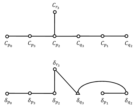
Figure 9: Generic $E_{7}$ intersection diagram at $s\neq 0$ (upper) and incomplete intersection diagram at $s=0$ (lower) of $E_{7}\rightarrow E_{8}$ : $p_{2}$-first ($p_{0}\rightarrow p_{1}\rightarrow p_{2}\rightarrow q_{3}$) case.

4.2 Complete resolution

We will now consider the complete resolution. This can be achieved by taking $f_{n+8}=s^{2}$ instead of $s$. This amounts to replacing $s$ in (125) with $s^{2}$. Similarly to the previous sections, we find an additional isolated codimension-two conifold singularity after we blow up $q_{3}$. As shown in red in Table 6, this new singularity, which we denote by $r_{4}$, arises at $(1:0:-1)$ on the $\hbox{\mybbsmall P}^{2}$ particularly at $s=0$. This adds an extra node to the incomplete intersection diagram to form the correct $E_{8}$ Dynkin diagram as we show in Figure 10. To see how the intersection matrix is modified, we repeat the argument given in section 3.2.2. By carefully lifting up ${\cal C}$’s and ${\delta}$’s into the local coordinate system of the small resolution, we find the modified relations

$${\cal C}_{p_{0}}= \delta_{p_{0}},$$ (161)

$${\cal C}_{p_{1}}= \delta_{p_{1}},$$

$${\cal C}_{p_{2}}= \delta_{p_{2}},$$

$${\cal C}_{q_{3}}= 2\delta_{q_{3}}+\delta_{r_{3}}+\delta_{q_{2}}+\delta_{\rm complete},$$

$${\cal C}_{r_{3}}= \delta_{r_{3}},$$

$${\cal C}_{q_{2}}= \delta_{q_{2}},$$

$${\cal C}_{p_{3}}= \delta_{p_{3}}.$$

One can then verify that: if the intersection matrix of these eight ${\delta}$’s is the minus of the ordinary $E_{8}$ Cartan matrix, the intersection matrix of ${\cal C}$’s (150) is reproduced. Therefore, the node $\delta_{q_{3}}$, which was formerly represented by a triangle in Figure 9, is now an ordinary node consisting of the root system of $E_{8}$ as in Figure 10.

Table 6: $E_{7}\rightarrow E_{8}$: Complete case when $p_{2}$ is blown up first ($p_{0}\to p_{1}\to p_{2}\to q_{3}$).

	1st blow up	2nd blow up	3rd blow up
\normalsize{$p_0$}⃝$\rightarrow$	\normalsize{$p_1(0:0:1)$}⃝$\rightarrow$	\normalsize{$p_2(1:0:0)$}⃝$\rightarrow$	\normalsize{$p_3(1:0:0)$}⃝$\rightarrow$
			\normalsize{$q_3(0:0:1)$}⃝$\rightarrow$
		$q_{2}(1:0:-s^{2})$	$q_{2}(0:0:1)(z_{2}=-s^{2})$
			$r_{3}(-s^{2}:0:1)$

4th blow up	5th blow up
regular
\normalsize{$r_4(1:0:-1;s=0)$}⃝$\mbox{(codim.2)}\rightarrow$	regular
\normalsize{$q_2(0:0:1)(z_2=-s^2)$}⃝$\rightarrow$	regular
\normalsize{$r_3(1:0:0)(x_3=-s^2)$}⃝$\rightarrow$	regular

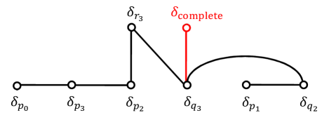
Figure 10: Complete $E_{8}$ intersection diagram of $E_{7}\rightarrow E_{8}$ : $p_{2}$-first ($p_{0}\rightarrow p_{1}\rightarrow p_{2}\rightarrow q_{3}$) case.

4.3 Incomplete/complete resolutions: Blowing up $q_{2}$ first

As we did for $SO(12)\rightarrow E_{7}$, we can change the order of the blow-ups to obtain a different intersection diagram. For instance, we can choose $q_{2}$ instead of $p_{2}$ for the 3rd blow up. The procedures are analogous to the previous cases so we report only the results.

For the incomplete resolution, the whole process of the blow-ups is as shown in Table 7. We use the same notation for ${\cal C}$’s (and hence for $\delta$’s) as was used in the $p_{2}$-first case. Then the intersection pattern of ${\cal C}$’s for the $q_{2}$-first case is the same $E_{7}$ Dynkin diagram with the $p_{2}$-first case given in Figure 9 and their intersection matrix is also the same with (150). The intersection pattern of $\delta$’s, however, is different from the one ($A_{7}$) given in Figure 9. This time, it is $E_{7}$ (see Figure 11 below).

One can verify the relations

$${\cal C}_{p_{0}}= \delta_{p_{0}}+\delta_{q_{2}},$$ (162)

$${\cal C}_{p_{1}}= \delta_{p_{1}},$$

$${\cal C}_{q_{2}}= 2\delta_{q_{2}}+2\delta_{p_{2}}+2\delta_{p_{3}}+\delta_{q_{3}}+\delta_{r_{3}},$$

$${\cal C}_{p_{2}}= \delta_{p_{2}},$$

$${\cal C}_{p_{3}}= \delta_{p_{3}},$$

$${\cal C}_{q_{3}}= \delta_{q_{3}},$$

$${\cal C}_{r_{3}}= \delta_{r_{3}}.$$

Then the intersection matrix among $\delta$’s has two $-\frac{3}{2}$ nodes as shown in Figure 11. The intersection among these two nodes is $\frac{1}{2}$. As is the same as the previous examples, one can form $28+28$ different linear combinations of $\delta$’s with non-negative and non-positive integer coefficients such that they have self-intersection $-\frac{3}{2}$, giving a single ${\bf 56}$ representation.

Table 7: $E_{7}\rightarrow E_{8}$: Incomplete case when $q_{2}$ is blown up first ($p_{0}\to p_{1}\to q_{2}$).

	1st blow up	2nd blow up	3rd blow up	4th blow up	5th blow up
\normalsize{$p_0$}⃝$\rightarrow$	\normalsize{$p_1(0:0:1)$}⃝$\rightarrow$	\normalsize{$q_2(1:0:-s)$}⃝$\rightarrow$	regular
		$p_{2}(1:0:0)$	\normalsize{$p_2(0:0:1)$}⃝$(\tilde{z}_{2}=s)\rightarrow$	\normalsize{$p_3(1:0:0)$}⃝$\rightarrow$	regular
				\normalsize{$q_3(0:0:1)$}⃝$\rightarrow$	regular
				\normalsize{$r_3(1:0:-1)$}⃝$\rightarrow$	regular

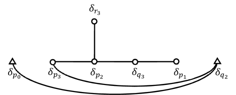
Figure 11: Incomplete intersection diagram of $E_{7}\rightarrow E_{8}$ : $q_{2}$-first ($p_{0}\rightarrow p_{1}\rightarrow q_{2}$) case.

In the complete case, the 3rd blow up at $q_{2}$ does not end with a smooth configuration but an isolated codimension-two conifold singularity remains at the intersection of $\delta_{p_{0}}$ and $\delta_{q_{2}}$ at $s=0$ (see Table 8). By a small resolution of this, the relations are modified as

$${\cal C}_{p_{0}}= \delta_{p_{0}}+\delta_{q_{2}}+\delta_{\rm complete},$$ (163)

$${\cal C}_{p_{1}}= \delta_{p_{1}},$$

$${\cal C}_{q_{2}}= 2\delta_{q_{2}}+2\delta_{p_{2}}+2\delta_{p_{3}}+\delta_{q_{3}}+\delta_{r_{3}}+\delta_{\rm complete},$$

$${\cal C}_{p_{2}}= \delta_{p_{2}},$$

$${\cal C}_{p_{3}}= \delta_{p_{3}},$$

$${\cal C}_{q_{3}}= \delta_{q_{3}},$$

$${\cal C}_{r_{3}}= \delta_{r_{3}}.$$

Demanding that the intersection matrix among $\delta$’s is the minus of the proper $E_{8}$ Cartan matrix is consistent with the intersection matrix among ${\cal C}$’s. As a result, we obtain Figure 12.

Table 8: $E_{7}\rightarrow E_{8}$: Complete case when $q_{2}$ is blown up first ($p_{0}\to p_{1}\to q_{2}$).

	1st blow up	2nd blow up	3rd blow up
\normalsize{$p_0$}⃝$\rightarrow$	\normalsize{$p_1(0:0:1)$}⃝$\rightarrow$	\normalsize{$q_2(1:0:-s)$}⃝$\rightarrow$	\normalsize{$p_4(1:0:0;s=0)$}⃝$\mbox{(codim.2)}\rightarrow$
		$p_{2}(1:0:0)$	\normalsize{$p_2(0:0:1)$}⃝$(\tilde{z}_{2}=s)\rightarrow$

4th blow up	5th blow up
regular
\normalsize{$p_3(1:0:0)$}⃝$\rightarrow$	regular
\normalsize{$q_3(0:0:1)$}⃝$\rightarrow$	regular
\normalsize{$r_3(1:0:-1)$}⃝$\rightarrow$	regular

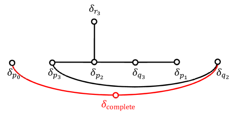
Figure 12: Complete $E_{8}$ intersection diagram of $E_{7}\rightarrow E_{8}$ : $q_{2}$-first ($p_{0}\rightarrow p_{1}\rightarrow q_{2}$) case.

4.4 Other inequivalent orderings

Let us summarize what other types of intersection diagrams are obtained for the enhancement $E_{7}\rightarrow E_{8}$ if we choose other orderings of the blow-ups. So far, we have derived the intersection diagrams for blow-ups with orders $p_{0}\rightarrow p_{1}\rightarrow p_{2}\rightarrow q_{3}$ and $p_{0}\rightarrow p_{1}\rightarrow q_{2}$. As we can see in the column “3rd blow up” in Table 5, after blowing up $p_{2}$, the three singular points $q_{3}$, $q_{2}$ and $r_{3}$ become an identical point $(0:0:1)$ on the $\hbox{\mybbsmall P}^{2}$ at $s=0$ (see also (131)). Therefore, besides the case when $q_{3}$ is blown up after $p_{2}$ as discussed in sections 4.1 and 4.2 , there are two other options: We can blow up either $q_{2}$ or $r_{3}$ after the blow up of $p_{2}$.

$p_{0}\rightarrow p_{1}\rightarrow p_{2}\rightarrow q_{2}$ case

If we blow up $q_{2}$ after $p_{2}$, the relations between ${\cal C}$’s and $\delta$’s are given by

$${\cal C}_{p_{0}}= \delta_{p_{0}},$$ (164)

$${\cal C}_{p_{1}}= \delta_{p_{1}},$$

$${\cal C}_{p_{2}}= \delta_{p_{2}}+\delta_{q_{2}}\,(+\delta_{\scriptsize\mbox{complete}}),$$

$${\cal C}_{q_{2}}= 2\delta_{q_{2}}+\delta_{q_{3}}+\delta_{r_{3}}\,(+\delta_{\scriptsize\mbox{complete}}),$$

$${\cal C}_{q_{3}}= \delta_{q_{3}},$$

$${\cal C}_{r_{3}}= \delta_{r_{3}},$$

$${\cal C}_{p_{3}}= \delta_{p_{3}}.$$

The intersection diagram of ${\cal C}$’s is the $E_{7}$ Dynkin diagram as before. The intersection diagrams of $\delta$’s for incomplete / complete cases are shown in Figure 13. For the incomplete case, it is an $E_{7}$ non-Dynkin diagram with two $-\frac{3}{2}$ nodes (the intersection among them is $\frac{1}{2}$), while for the complete case, it is proper $E_{8}$ Dynkin diagram. Again, there is only one ${\bf 56}$ at $s=0$ as two-cycles $J$ (78) with $J\cdot J=-\frac{3}{2}$.

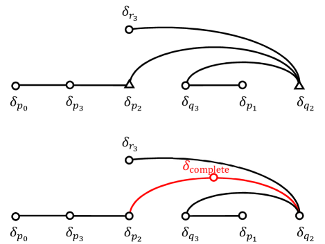
Figure 13: Incomplete/complete intersection diagrams of $E_{7}\rightarrow E_{8}$ : $p_{2}$-first ($p_{0}\rightarrow p_{1}\rightarrow p_{2}\rightarrow q_{2}$) case.

$p_{0}\rightarrow p_{1}\rightarrow p_{2}\rightarrow r_{3}$ case

If we blow up $r_{3}$ after $p_{2}$, the relations between ${\cal C}$’s and $\delta$’s are given by

$${\cal C}_{p_{0}}= \delta_{p_{0}},$$ (165)

$${\cal C}_{p_{1}}= \delta_{p_{1}}+\delta_{r_{3}}\,(+\delta_{\scriptsize\mbox{complete}}),$$

$${\cal C}_{p_{2}}= \delta_{p_{2}},$$

$${\cal C}_{r_{3}}= 2\delta_{r_{3}}+\delta_{q_{2}}+\delta_{q_{3}}\,(+\delta_{\scriptsize\mbox{complete}}),$$

$${\cal C}_{q_{2}}= \delta_{q_{2}},$$

$${\cal C}_{q_{3}}= \delta_{q_{3}},$$

$${\cal C}_{p_{3}}= \delta_{p_{3}}.$$

The intersection diagrams are shown in Figure 14. The diagram for the incomplete case is a $D_{7}$ non-Dynkin diagram with two $-\frac{3}{2}$ nodes (their intersection is $\frac{1}{2}$). Again, there is only one ${\bf 56}$ at $s=0$.

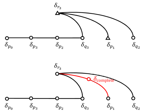
Figure 14: Incomplete/complete intersection diagrams of $E_{7}\rightarrow E_{8}$ : $p_{2}$-first ($p_{0}\rightarrow p_{1}\rightarrow p_{2}\rightarrow r_{3}$) case.

This exhausts all the possibilities of changing the order of the singularities we blow up. We obtained four sets of incomplete / complete intersection diagrams. Again, each of them corresponds to a box graph on every other row of Figure 44 in BoxGraphs . For the $p_{2}$-first cases, Figure 9 (with Figure 10) is equivalent to the one in the right column: Figure 13 and Figure 14 respectively are the fourth and sixth ones from the bottom in the left column. For the $q_{2}$-first case, Figure 11 (with Figure 12) is the second one from the bottom in the left column.

5 Conclusions

We have investigated the resolutions of codimension-two enhanced singularities from $SO(12)$ to $E_{7}$ and from $E_{7}$ to $E_{8}$ in six-dimensional F-theory, where a half-hypermultiplet locally arises for generic complex structures achieving them. A half-hypermultiplet only occurs associated with a Lie algebra allowing a pseudo-real representation, and the above are the two of the three cases in the list of six-dimensional F-theory compactifications BIKMSV that exhibit half-hypermultiplets in the massless matter spectrum. As was already observed in the enhancement from $SU(6)$ to $E_{6}$ in MT , we have confirmed that the resolution process does not generically yield as many number of exceptional curves as naively expected from the Kodaira classification of the codimension-one singularities. In the present paper, we have observed similar features such as non-Dynkin intersection diagrams and half-integral intersection numbers of exceptional fibers. Then we have found that the exceptional fibers at the enhanced point form extremal rays of the cone of the positive weights of the relevant pseudo-real representation, explaining why a half-hyper multiplet arises there.

We have also found that a variety of different intersection diagrams of exceptional curves are obtained by altering the ordering of the singularities blown up in the process. They correspond to different “phases” of the three-dimensional M-theory. We have obtained, for both $SO(12)\rightarrow E_{7}$ and $E_{7}\rightarrow E_{8}$, the intersection diagram on every other row of the figures in BoxGraphs , but not all of them. The phases corresponding to the diagrams we obtained are not the ones related by a flop.

We have presented detailed derivations of the intersection diagrams of the exceptional fibers at the singularity enhanced points. In particular, we have described how an exceptional curve is lifted up on the chart arising due to the subsequent blowing-up process. By carefully examining whether an exceptional curve contains another arising afterwards as a part, we have obtained the intersection matrices as above.

In the complete resolutions, where the colliding brane approaches the stack of branes as $O(s^{2})$, we have obtained the full Dynkin diagrams of the group $G$ as the intersection diagram of the fibers at the enhanced point. The extra codimension-two singularity is always a conifold singularity, as was found in the previous example MT .

Although we have studied in this paper the explicit resolutions of the singularities in six dimensions, the technologies we have developed here can also be used in more general settings such as codimension-three singularities in Calabi-Yau four-folds, with or without sections. (In the latter, one may consider the Jacobian fibrations. See e.g. Kimura . )

It would also be interesting to perform a similar analysis for a singularity with higher rank enhancement. In particular, it has been expected FFamilyUnification that a codimension-three singularity enhancement from $SU(5)$ to $E_{7}$ could yield, without monodromies and with appropriate $G$-fluxes, the three-generation spectrum of the $E_{7}/(SU(5)\times U(1)^{3})$ supersymmetric coset model KugoYanagida . Such a codimension-two singularity enhancement in six dimensions was already studied in MizoguchiTanianomaly . The codimension-three case with a $\hbox{\mybbsmall Z}_{2}$ or a larger monodromy was considered in e.g. HTV , but was concluded to be not very useful for their purposes. The box graph analysis of BoxGraphs , on the other hand, predicts the existence of the phases without monodromies, which will serve as basis for models of family unification in F-theory. We hope to come back to this issue elsewhere.

Finally, massless matter generation in F-theory may also be explained by string junctions stretched between various $(p,q)$ 7-branes near the intersections. Very recently, a new pictorial method to keep track of non-localness of F-theory 7-branes has been developed by drawing a “dessin” on the base of the elliptic fibration dessin1 ; dessin2 , which may help understanding how the difference of the resolutions is affected by the geometry near the enhanced point.

Appendix A Symplectic Majorana-Weyl spinors, pseudo-real representations and half-hypermultiplets

A.1 Symplectic Majorana-Weyl spinors

In six(=5+1) dimensions, consider the Dirac equation

$$(i\gamma^{\mu}\partial_{\mu}-m)\psi = 0.$$ (166)

The complex conjugate equation

$$(-i\gamma^{\mu*}\partial_{\mu}-m)\psi^{*} = 0$$ (167)

can be written in terms of the charge conjugation $\psi^{c}$ defined by

$$\psi^{c}\equiv B\psi^{*}$$ (168)

with

$$B\gamma^{\mu*}B^{-1}=-\gamma^{\mu}$$ (169)

as

$$(i\gamma^{\mu}\partial_{\mu}-m)\psi^{c} = 0.$$ (170)

This is the same Dirac equation as that $\psi$ obeys. If one could impose the constraint $\psi^{c}=\psi$ on $\psi$, one could define a Majorana spinor, but in six dimensions one can not as, if one could do so,

$$\psi=\psi^{c}=B\psi^{*}=B(B\psi^{*})^{*}=BB^{*}\psi,$$ (171)

but

$$BB^{*} = -1$$ (172)

in six dimensions. Alternatively, one can impose on two Weyl spinors $\psi_{1}$, $\psi_{2}$ the constraint

$$\psi^{c}_{1}=+\psi_{2},~{}~{}~{}\psi^{c}_{2}=-\psi_{1}.$$ (173)

They are called symplectic Majorana-Weyl spinors. Note that in six(=5+1)-dimensions the charge conjugation operation does not flip the chirality so that one can define symplectic Majorana-Weyl spinors.

A.2 Pseudo-real representation and symplectic Majorana condition

Let us examine whether one can consistently impose this constraint on a representation space of a Lie group. Let $G$ be a compact Lie group and $\rho$ be its representation on a complex $2n$-dimensional vector space $V$:

$$\rho:G\rightarrow GL_{\hbox{\mybbsub C}}(V)~{}~{}~{}\mbox{homomorphism}.$$ (174)

We say $\rho$ is a pseudo-real representation if there exists $P\in GL_{\hbox{\mybbsub C}}(V)$ such that

$$P(\rho(g))^{*}P^{-1} = \rho(g)$$ (175)

for any $g\in G$. ^∗ denotes the complex conjugation.

If

$$v^{\prime} = \rho(g)v,$$ (176)

then

$$Pv^{\prime*} = (P(\rho(g))^{*}P^{-1})Pv^{*}$$ (177)

$$= \rho(g)Pv^{*}.$$

Therefore $Pv^{*}$ also transforms as 2n.

If $\rho(g)$ can be embedded in $Sp(2n)$, we have

$$\rho(g)^{T}\Omega_{2n}\rho(g) = \Omega_{2n},$$

$$\Omega_{2n} = \left(\begin{array}[]{cc}0&-1_{n}\\ 1_{n}&0\end{array}\right).$$ (180)

Moreover, if $\rho$ is a unitary representation: $\rho(g)^{-1}=\rho(g)^{\dagger}$, we find

$$\rho(g) = \Omega_{2n}\rho(g)^{*}\Omega_{2n}^{-1}.$$ (181)

Thus we can take

$$P=\Omega_{2n}.$$ (182)

Let us construct such a vector $v$ by using symplectic Majorana(-Weyl) spinors. Let $\psi_{1}$, $\psi_{2}$ be a pair of $n$-component column vectors consisting of $n$ symplectic Majorana(-Weyl) spinors, and $v$ be a stack of them. Then

$$v = \left(\begin{array}[]{c}\psi_{1}\\ \psi_{2}\end{array}\right)$$ (185)

$$= \left(\begin{array}[]{c}-\psi^{c}_{2}\\ \psi^{c}_{1}\end{array}\right)$$ (188)

$$= \left(\begin{array}[]{cc}0&-1_{n}\\ 1_{n}&0\end{array}\right)\left(\begin{array}[]{c}\psi^{c}_{1}\\ \psi^{c}_{2}\end{array}\right)$$ (193)

$$= \Omega_{2n}\left(\begin{array}[]{c}B\psi^{*}_{1}\\ B\psi^{*}_{2}\end{array}\right)$$ (196)

$$= \Omega_{2n}(B\cdot 1_{2n})v^{*}.$$ (197)

In general, this is not consistent as $v$ transforms as a ${\bf 2n}$ representation whereas $v^{*}$ as a $\overline{\bf 2n}$ representation. However, for a pseudo-real representation (181), we obtain

$$\rho(g)v = \Omega_{2n}\rho(g)^{*}\Omega_{2n}^{-1}\cdot\Omega_{2n}(B\cdot 1_{2n})v^{*}$$ (198)

$$= \Omega_{2n}(B\cdot 1_{2n})\rho(g)^{*}v^{*},$$

which agrees with (197). Therefore, for a pseudo-real representation a $2n$-dimensional representation space can be constructed from $n$ pairs of symplectic Majorana-Weyl spinors.

A.3 $\frac{\bf 2n}{2}$ hypermultiplets vs. ${\bf 2n}$ $\frac{1}{2}$hypermultiplets

In the previous section we have seen that among $2n$ Weyl fermions in hypermultiplets transforming as a pseudo-real ${\bf 2n}$ representation one half ($=n$) of them can be expressed as the complex conjugates of the other half ($=n$). In this section we will show that this can be viewed as a restriction of the degrees of freedom of $2n$ (Weyl fermions of) hypermultiplets to $2n$ (“half-Weyl” fermions of) half-hypermultiplets.

We take

$$\Gamma^{0} = \sigma_{3}\otimes\sigma_{3}\otimes i\sigma_{2},$$

$$\Gamma^{1} = \sigma_{3}\otimes\sigma_{3}\otimes\sigma_{1},$$

$$\Gamma^{2} = \sigma_{3}\otimes\sigma_{1}\otimes 1,$$

$$\Gamma^{3} = \sigma_{3}\otimes\sigma_{2}\otimes 1,$$

$$\Gamma^{4} = \sigma_{1}\otimes 1\otimes 1,$$

$$\Gamma^{5} = \sigma_{2}\otimes 1\otimes 1$$ (199)

as a realization of the gamma matrices. As the matrix $B$ satisfying (169), we can have

$$B = \Gamma^{0}\Gamma^{1}\Gamma^{2}\Gamma^{4}.$$ (200)

Since

$$\Gamma^{0}\Gamma^{1}\Gamma^{2} = \sigma_{3}\otimes\sigma_{1}\otimes\sigma_{3},$$ (201)

we can write $B$ in a block form as

$$B = \left(\begin{array}[]{cc}b&0\\ 0&-b\end{array}\right)\left(\begin{array}[]{cc}0&{\bf 1}\\ {\bf 1}&0\end{array}\right),$$ (206)

where

$$\sigma_{1}\otimes\sigma_{3} \equiv b.$$ (207)

1 is the $4\times 4$ unit matrix.

Since the chirality in six dimensions is defined by

$$\Gamma^{\sharp}~{}\equiv~{}-\Gamma^{0}\Gamma^{1}\Gamma^{2}\Gamma^{3}\Gamma^{4}\Gamma^{5} \equiv (\sigma_{3}\otimes{\bf 1})({\bf 1}\otimes\gamma_{5}),$$ (208)

the eigenvalues of $\gamma_{5}$ and $(\sigma_{3}\otimes{\bf 1})$ are correlated with each other in a six-dimensional spinor with a definite chirality. For instance, if $\Gamma^{\sharp}=+1$, $(\gamma_{5},\sigma_{3})=(+,+)$ or $(-,-)$. Thus if we write

$$\psi_{i} = \left(\begin{array}[]{c}\phi_{i}\\ \chi_{i}\end{array}\right)~{}~{}~{}(i=1,2),$$ (211)

this is a decomposition with respect to the four-dimensional chirality. From (206), we have

$$\psi_{i}^{c} = B\psi_{i}^{*}$$ (218)

$$= \left(\begin{array}[]{cc}b&0\\ 0&-b\end{array}\right)\left(\begin{array}[]{cc}0&{\bf 1}\\ {\bf 1}&0\end{array}\right)\left(\begin{array}[]{c}\phi_{i}^{*}\\ \chi_{i}^{*}\end{array}\right)$$

$$= \left(\begin{array}[]{r}b\chi_{i}^{*}\\ -b\phi_{i}^{*}\end{array}\right).$$ (221)

Therefore, if a collection of $n$ spinors $\psi_{2}$ are written as $\psi_{1}^{c}$, the relations $\psi_{2}=\psi_{1}^{c}$ and $\psi_{1}=-\psi_{2}^{c}$ imply

$$\chi_{2}=-b\phi_{1}^{*},~{}~{}~{}\chi_{1}=+b\phi_{2}^{*}.$$ (222)

Thus the lower component of each of the $2n$ Weyl spinors can be expressed in terms of the upper component.

A.4 Restriction on the complex scalars

Let $v_{i}$ $(i=1,2)$ be a pair of $n$ complex scalars and

$$\left(\begin{array}[]{c}v_{1}\\ v_{2}\end{array}\right)$$ (225)

be in the ${\bf 2n}$ pseudo-real representation of $G$. In order to similarly define $v_{i}^{c}$ such that

$$v_{2}=v_{1}^{c},~{}~{}~{}v_{1}=-v_{2}^{c}$$ (226)

by

$$v_{i}^{c} \equiv Uv^{*}_{i}$$ (227)

for some $U$ satisfying $U^{*}U=-1$, we recall that a hypermultiplet has two complex scalars transforming in the identical representation. Let $v^{(1)}_{i}$ and $v^{(2)}_{i}$ be such two scalars, then writing $v_{i}=\left(\begin{array}[]{c}v^{(1)}_{i}\\ v^{(2)}_{i}\end{array}\right)$, we define

$$v_{i}^{c} = \left(\begin{array}[]{c}v^{(1)c}_{i}\\ v^{(2)c}_{i}\end{array}\right)$$ (230)

$$\equiv U\left(\begin{array}[]{c}v^{(1)*}_{i}\\ v^{(2)*}_{i}\end{array}\right),$$ (233)

where

$$U \equiv \left(\begin{array}[]{cc}0&-1\\ 1&0\end{array}\right)$$ (236)

is a $90^{\circ}$ $U(1)_{R}$ rotation. Then $U^{*}U=-1$, and (226) can be imposed. With this definition of $v_{i}^{c}$, one can also reduce the degrees of freedom of the complex scalars in a hypermultiplet.

Appendix B Summary of $SU(6)\rightarrow E_{6}$

In this appendix we summarize the results of the analysis MT of the codimension-two enhancement $SU(6)\rightarrow E_{6}$. Consider

$$\Phi = -y^{2}+x^{3}+(t_{r}^{2}+3t_{r}z)x^{2}+(2t_{r}z^{2}+3z^{3})x+z^{4}.$$ (237)

One can verify that $\Phi$ has an $SU(6)$ singularity at $(x,y,z)$ for fixed $t_{r}\neq 0$, and this is enhanced to an $E_{6}$ singularity for $t_{r}=0$. $\Phi$ (237) can be obtained by putting $h_{n+2-r}=\frac{1}{\sqrt{3}}$, $H_{n+4-r}=-\frac{1}{2}$, $u_{r+4}=\frac{1}{2}$, $f_{n+8-r}=f_{8}=g_{12}=0$ in (10) and (11) and making a change of variables.

If we take $t_{r}=s$, we are led to the incomplete resolution. The process is summarized in Table 9. After the codimension-one blow up at the singularity $p_{0}$ of $\Phi$ (237), we obtain two exceptional curves ${\cal C}_{1\pm}$ at fixed $s\neq 0$, which come on top of each other into a single curve $\delta_{1}$ at $s=0$. These two curves intersect at a singularity $p_{1}$, which forms a singular line along the $s$ direction. We perform a codimension-one blow up along this line to find, again, two exceptional curves ${\cal C}_{2\pm}$ at $s\neq 0$, which becomes $\delta_{2\pm}$ at $s=0$. The intersection of ${\cal C}_{2\pm}$ is again another singularity $p_{2}$. We then blow up the singularity line $p_{2}$ to get a regular curve ${\cal C}_{3}$ at $s\neq 0$, which splits into two curves $\delta_{3\pm}$ at $s=0$.

In the incomplete case, this is the end. The relations among ${\cal C}$’s and $\delta$’s are given by

$${\cal C}_{1\pm}=\delta_{1}+\delta_{3\pm},$$

$${\cal C}_{2\pm}=\delta_{2\pm},$$

$${\cal C}_{3}=\delta_{3+}+\delta_{3-}.$$ (238)

One can derive these relations in the same way as explained in section 3.1.3. Their intersection diagrams are shown in Figure 15.

Table 9: $SU(6)\rightarrow E_{6}$: Incomplete case.

	1st blow up	2nd blow up	3rd blow up
\normalsize{$p_0$}⃝$\rightarrow$	\normalsize{$p_1(0:0:1)$}⃝$\rightarrow$	\normalsize{$p_2(1:0:-s)$}⃝$\rightarrow$	regular

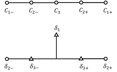
Figure 15: Generic intersection diagram at $s\neq 0$ (upper) and incomplete intersection diagram at $s=0$ (lower) of $SU(6)\rightarrow E_{6}$.

For the complete resolution, we take $t_{r}=s^{2}$. In this case, as is shown in Table 10, we have an additional codimension-two isolated conifold singularity after the 3rd blow up.

The relations (238) are modified to

$${\cal C}_{1\pm}=\delta_{1}+\delta_{3\pm}+\delta_{\rm complete},$$

$${\cal C}_{2\pm}=\delta_{2\pm},$$

$${\cal C}_{3}=\delta_{3+}+\delta_{3-}+\delta_{\rm complete}.$$ (239)

This result is obtained by following the analysis explained in section 3.2.2. The intersection diagram of these six $\delta$’s is the proper $E_{6}$ Dynkin diagram as in Figure 16.

Table 10: $SU(6)\rightarrow E_{6}$: Complete case.

	1st blow up	2nd blow up	3rd blow up	4th blow up
\normalsize{$p_0$}⃝$\rightarrow$	\normalsize{$p_1(0:0:1)$}⃝$\rightarrow$	\normalsize{$p_2(1:0:-w)$}⃝$\rightarrow$	\normalsize{$p_3(1:0:0;s=0)$}⃝$\mbox{(codim.2)}\rightarrow$	regular

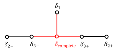
Figure 16: Complete $E_{6}$ intersection diagram of $SU(6)\rightarrow E_{6}$.

Appendix C Small resolution of a conifold singularity

In this appendix, we give a brief review of the small resolution (see, e.g., CD ). A conifold ${\cal M}$ is a three dimensional space given by the polynomial in $\hbox{\mybbsmall C}^{4}$

$$X_{1}X_{4}-X_{2}X_{3}=0.$$ (240)

It has a singularity at $(X_{1},X_{2},X_{3},X_{4})=(0,0,0,0)$, which is called the conifold singularity. In general, an isolated singularity on a hypersurface in $\hbox{\mybbsmall C}^{4}$ can be resolved by inserting $\hbox{\mybbsmall P}^{3}$ in the ambient space $\hbox{\mybbsmall C}^{4}$. For the conifold singularity, it is equivalent to inserting $\hbox{\mybbsmall P}^{1}\times\hbox{\mybbsmall P}^{1}$ on the conifold ${\cal M}$. However, it is sufficient to insert only one $\hbox{\mybbsmall P}^{1}$ to resolve the conifold singularity. This process is called the small resolution. Inserting $\hbox{\mybbsmall P}^{1}$ at the origin of ${\cal M}$ is given by

$$\breve{\cal M}=\left\{(X_{1},X_{2},X_{3},X_{4})\times(y_{1}:y_{2})\begin{array}[]{r|}\\ \\ \end{array}\left[\begin{array}[]{cc}X_{1}&X_{2}\\ X_{3}&X_{4}\end{array}\right]\left[\begin{array}[]{c}y_{1}\\ y_{2}\end{array}\right]=\left[\begin{array}[]{c}0\\ 0\end{array}\right]\right\}.$$ (241)

Let us write $M={\small\left[\begin{array}[]{rl}X_{1}&X_{2}\\ X_{3}&X_{4}\end{array}\right]}.$ Since $(y_{1}:y_{2})\neq(0,0)$, $\mbox{det}M=0$. This gives the defining equation of the conifold (240). Furthermore, if

$$\begin{split}(X_{1},X_{2},X_{3},X_{4})\left\{\begin{array}[]{l}\neq(0,0,0,0)\Rightarrow\mbox{rank}M=1\Rightarrow(y_{1}:y_{2})\mbox{ is determined,}\\ =(0,0,0,0)\Rightarrow\mbox{rank}M=0\Rightarrow(y_{1}:y_{2})\mbox{ is undetermined,}\end{array}\right.\end{split}$$

which means that $\hbox{\mybbsmall P}^{1}=(y_{1}:y_{2})$ is inserted only at the origin. As a result, $\breve{\cal M}$ is regular, since $\partial_{X_{1}}(X_{1}y_{1}+X_{2}y_{2})=y_{1}=0$ and $\partial_{X_{2}}(X_{1}y_{1}+X_{2}y_{2})=y_{2}=0$ are not compatible.

$\breve{\cal M}$ is covered by two local coordinate patches. If $y_{1}\neq 0$, we can solve (241) as

$$X_{1}=-\frac{y_{2}}{y_{1}}X_{2}\,\,,\,\,X_{3}=-\frac{y_{2}}{y_{1}}X_{4},$$ (242)

and hence

$$(X_{1},X_{2},X_{3},X_{4})=(-\lambda X_{2},X_{2},-\lambda X_{4},X_{4})\quad\mbox{with}\,\,\lambda\equiv\frac{y_{2}}{y_{1}}.$$ (243)

We call this patch $H_{+}$. Local coordinates of $H_{+}$ are $(X_{2},X_{4},\lambda)$ and the inserted $\hbox{\mybbsmall P}^{1}=(y_{1}:y_{2})$ is located at

$$(X_{2},X_{4},\lambda)=(0,0,\lambda).$$ (244)

If $y_{2}\neq 0$, we can solve (241) as

$$X_{2}=-\frac{y_{1}}{y_{2}}X_{1}\,\,,\,\,X_{4}=-\frac{y_{1}}{y_{2}}X_{3},$$ (245)

and hence

$$(X_{1},X_{2},X_{3},X_{4})=(X_{1},-\mu X_{1},X_{3},-\mu X_{3})\quad\mbox{with}\,\,\mu\equiv\frac{y_{1}}{y_{2}}.$$ (246)

We call this patch $H_{-}$. Local coordinates of $H_{-}$ are $(X_{1},X_{3},\mu)$ and the inserted $\hbox{\mybbsmall P}^{1}$ is

$$(X_{1},X_{3},\mu)=(0,0,\mu).$$ (247)

References

- (1) C. Vafa, Nucl. Phys. B 469, 403 (1996) [hep-th/9602022].
- (2) E. Witten, Nucl. Phys. B 471 (1996) 135
- (3) R. Blumenhagen, B. Kor̈ s, D. Lus̈t, and T. Ott, Nucl. Phys. B 616, 3–33 (2001) [hep-th/0107138].
- (4) R. Blumenhagen, M. Cvetič, D. Lus̈t, R. Richter, and T. Weigand, Phys. Rev. Lett. 100 (2008) 061602, 0707.1871.
- (5) D. R. Morrison and C. Vafa, Nucl. Phys. B 473, 74 (1996) [hep-th/9602114].
- (6) D. R. Morrison and C. Vafa, Nucl. Phys. B 476, 437 (1996) [hep-th/9603161].
- (7) M. Bershadsky, K. Intriligator, S. Kachru, D.R. Morrison, V. Sadov and C. Vafa, Nucl.Phys. B481 (1996) 215-252 [hep-th/9605200].
- (8) S. H. Katz and C. Vafa, Nucl. Phys. B 497, 146 (1997) [hep-th/9606086].
- (9) T. Tani, Nucl. Phys. B 602, 434 (2001).
- (10) S. Mizoguchi, JHEP 1407, 018 (2014) [arXiv:1403.7066 [hep-th]].
- (11) D. R. Morrison and W. Taylor, JHEP 1201, 022 (2012) [arXiv:1106.3563 [hep-th]].
- (12) M. Gunaydin, G. Sierra and P. K. Townsend, Phys. Lett. B 133 (1983) 72.
- (13) M. Gunaydin, G. Sierra and P. K. Townsend, Nucl. Phys. B 242 (1984) 244.
- (14) H. Hayashi, C. Lawrie, D. R. Morrison and S. Schafer-Nameki, JHEP 1405, 048 (2014) [arXiv:1402.2653 [hep-th]].
- (15) M. Esole and S. T. Yau, Adv. Theor. Math. Phys. 17, no. 6, 1195 (2013) [arXiv:1107.0733 [hep-th]].
- (16) J. Marsano and S. Schafer-Nameki, JHEP 1111, 098 (2011) [arXiv:1108.1794 [hep-th]].
- (17) M. Esole, S. H. Shao and S. T. Yau, Adv. Theor. Math. Phys. 19, no. 6, 1183 (2015) [arXiv: 1402.6331 [hep-th]]; Adv. Theor. Math. Phys. 20, no. 4, 683 (2016) [arXiv: 1407.1867 [hep-th]].
- (18) A. P. Braun and S. Schafer-Nameki, Nucl. Phys. B 905 (2016) 447 [arXiv:1407.3520 [hep-th]]; Nucl. Phys. B 905 (2016) 480 [arXiv:1511.01801 [hep-th]].
- (19) H. Pinkham, in Singularities (P. Orlik, ed.), vol. 40, part 2 of Proc. Symp. Pure Math., pp. 343-371, American Mathematical Society, 1983.
- (20) M. Reid, in Algebraic Varieties and Analytic Varieties (S. Iitaka, ed.), vol. 1 of Adv. Stud. Pure Math., pp. 131-180, Kinokuniya, 1983.
- (21) S. Katz and D. R. Morrison, J. Algebraic Geom. 1 (1992) 449-530, [arXiv:alg-geom/9202002].
- (22) R. Friedman, J. Morgan and E. Witten, Commun. Math. Phys. 187, 679 (1997) [hep-th/9701162].
- (23) R. Donagi and M. Wijnholt, Adv. Theor. Math. Phys. 15, 1237 (2011) [arXiv:0802.2969 [hep-th]].
- (24) S. Mizoguchi and T. Tani, JHEP 1611, 053 (2016) [arXiv:1607.07280 [hep-th]].
- (25) K. Oguiso and T. Shioda, Comment. Math. Univ. St. Pauli. 40 (1991) 83.
- (26) P. Candelas and X. C. de la Ossa, Nucl. Phys. B 342 (1990) 246-268.
- (27) Y. Kimura, JHEP 1704, 168 (2017) [arXiv:1608.07219 [hep-th]].
- (28) T. Kugo and T. Yanagida, Phys. Lett. 134B, 313 (1984). doi:10.1016/0370-2693(84)90007-8
- (29) S. Mizoguchi and T. Tani, PTEP 2016, no. 7, 073B05 (2016) [arXiv:1508.07423 [hep-th]].
- (30) J. J. Heckman, A. Tavanfar and C. Vafa, JHEP 1008, 040 (2010) [arXiv:0906.0581 [hep-th]].
- (31) S. Fukuchi, N. Kan, S. Mizoguchi and H. Tashiro, Phys. Rev. D 100, no. 12, 126025 (2019) [arXiv:1808.04135 [hep-th]].
- (32) S. Fukuchi, N. Kan, R. Kuramochi, S. Mizoguchi and H. Tashiro, Phys. Lett. B 803, 135333 (2020) [arXiv:1912.02974 [hep-th]].