Disentangling the formation history of galaxies via population-orbit superposition: method validation

Abstract

We present population-orbit superposition models for external galaxies based on Schwarzschild’s orbit-superposition method, by tagging the orbits with age and metallicity. The models fit the density distributions, as well as kinematic, age and metallicity maps from Integral Field Unit (IFU) spectroscopy observations. We validate the method and demonstrate its power by applying it to mock data, similar to those obtained by the Multi-Unit Spectroscopic Explorer (MUSE) IFU on the Very Large Telescope (VLT). These mock data are created from Auriga galaxy simulations, viewed at three different inclination angles ($\vartheta=40^{o},60^{o},80^{o}$). Constrained by MUSE-like mock data, our model can recover the galaxy’s stellar orbit distribution projected in orbital circularity $\lambda_{z}$ vs. radius $r$, the intrinsic stellar population distribution in age $t$ vs. metallicity $Z$, and the correlation between orbits’ circularity $\lambda_{z}$ and stellar age $t$. A physically motivated age-metallicity relation improves recovering the intrinsic stellar population distributions. We decompose galaxies into cold, warm and hot + counter-rotating components based on their orbit circularity distribution, and find that the surface density, mean velocity, velocity dispersion, age and metallicity maps of each component from our models well reproduce those from simulation, especially for projections close to edge-on. These galaxies exhibit strong global age vs. $\sigma_{z}$ relation, which is well recovered by our model. The method has the power to reveal the detailed build-up of stellar structures in galaxies, and offers a complement to local resolved, and high-redshift studies of galaxy evolution.

1 Introduction

Stellar dynamics provides a fossil record of the formation history of galaxies. Stars that were born and remain in quiescent environments tend to be on regular rotation-dominated orbits. On the other hand, stars born from turbulent gas or that have been dynamically heated after birth will be on warmer orbits with more random motions (Leaman et al., 2017). Stellar heating mechanisms include violent mergers (e.g. Benson et al., 2004; House et al., 2011; Helmi et al., 2012; Few et al., 2012; Ruiz-Lara et al., 2016) and long-term secular heating of the disk via internal instabilities (e.g. Jenkins & Binney, 1990; Aumer, Binney & Schönrich, 2016; Grand et al., 2016).

As the Universe evolves, a galaxy’s mass density, gas fraction and star formation all decrease. This likely reduces the velocity dispersion of the gas from which stars form, the mass spectrum of dense giant molecular clouds, and the frequency of mergers (Genzel et al., 2011; Wisnioski et al., 2015). Stellar kinematics are therefore expected for multiple reasons to be systematically correlated with stellar ages (Trayford et al., 2018). Several observations have revealed that old stars dominate the light of random-motion-dominated bulges, while younger stars live on thinner disks. Stars born during the same epoch tend to live on similar orbits (e.g., Bird et al. 2013, Stinson et al. 2013). At the present day, the stellar phase space distribution of a galaxy is thus a combination of stars formed over its lifetime. A mixture of merging events and star formation episodes determines the diversity of a galaxy’s structure and stellar populations.

Observationally, it is difficult to identify coherent structures in the density distribution and kinematics of stars formed at high redshift (van der Wel et al., 2016). Fortunately, the chemistry and age imprinted in a star provide coordinates of the time and environment of its birth. Taking the Milky Way (MW) as an example, the chemical abundance as well as the 6D phase-space information of a single star could be obtained by combining Gaia (Gaia Collaboration et al., 2018) and spectroscopic surveys. In the solar neighborhood, most stars are disk stars, which we can identify as they are on near-circular orbits, and are both young and metal-rich (e.g. Mackereth et al., 2017). Although spatially-coincident, we can also identify a small fraction of halo stars as they are on radial/vertical-motion-dominated orbits, and are old and metal-poor (e.g. Helmi et al., 2018; Belokurov et al., 2018, 2019). The chemical information of disk stars and halo stars gives us insight into the formation history of the MW (Helmi et al., 2018; Belokurov et al., 2018; Fattahi et al., 2019).

However, only a handful of galaxies are near enough for us to resolve their stars. For most external galaxies, all of our information comes from integrated light. In these cases, the spectrum we observe at each pixel is a light-weighted combination of spectra from all the stars along the line-of-sight, which come from different populations with different ages, metallicities and kinematics. By full spectrum fitting (e.g. Cappellari 2017), we can obtain the line-of-sight velocity distribution (LOSVD), which is usually described by a Gauss-Hermite (GH) profile with parameters of mean velocity ($V$), velocity dispersion ($\sigma$), and/or higher order GH coefficients, like the third and fourth order $h_{3}$ and $h_{4}$ or even higher $h_{5}$ and $h_{6}$. These full spectrum fits also return the average age and metallicity of the underlying stellar populations. Such methodologies have been applied in many Integral Field Unit (IFU) spectroscopic surveys, such as the Calar Alto Legacy Integral Field Area Survey (CALIFA; Sánchez et al. 2012), the Sydney AAO Multi-object Integral Field galaxy survey (SAMI; Croom et al. 2012), and the Mapping Nearby Galaxies at APO survey (MaNGA; Bundy et al. 2015). These surveys provide a spectrum at each pixel across the galaxy plane. From these spectra and the aforementioned techniques, we obtain kinematic maps ($V$, $\sigma$, $h_{3}$, $h_{4}$…), as well as age and metallicity maps.

Disentangling the different stellar populations in present-day galaxies, and the structures they form, will give us insight into the galaxy’s formation history; however this is challenging as it typically requires resolved stellar abundances and ages or deep integrated light spectroscopy (Leaman, VandenBerg & Mendel, 2013; Boecker et al., 2019). Full spectrum (or SED) fitting has been pushed to provide not only average stellar population properties, but a distribution of ages and metallicities - such as a star formation history (SFH) or age metallicity relation (AMR) (e.g. Cid Fernandes et al., 2005; Cappellari, 2017; Carnall et al., 2019; Leja et al., 2019; McDermid et al., 2015). Based on the SFH obtained at each pixel, galaxies can be decomposed into structures with different stellar ages and metallicities (Guérou et al. 2016, Pinna et al. 2019b, Pinna et al. 2019a, Pizzella et al. 2018, Tabor et al. 2019).

Dynamical models offer us an alternative and powerful tool to probe a galaxy’s formation history. The particle-based Made-to-Measure method (M2M de Lorenzi et al., 2007; Long & Mao, 2010; Hunt & Kawata, 2014) and the orbit-based Schwarzschild method (van der Marel & Franx, 1993; Rix et al., 1997; Cretton & van den Bosch, 1999; Gebhardt et al., 2000; Valluri, Merritt & Emsellem, 2004; van den Bosch et al., 2008; van de Ven, de Zeeuw & van den Bosch, 2008; Vasiliev & Valluri, 2019) probe how stars orbit in a gravitational potential without ad-hoc assumptions about the underlying orbital structures. The triaxial Schwarzschild model developed by van den Bosch et al. (2008) has proved to be effective at recovering the orbit distributions of a variety of galaxies (Zhu et al. 2018a; Zhu et al. 2018b; Jin et al. 2019). It has notably been applied to a large sample of 300 CALIFA galaxies in the local universe to recover their stellar orbit distributions (Zhu et al., 2018b). However, the orbits recovered in that study (and most others) are monochromatic and provide no information about the underlying stellar populations.

Recently, there have been a few pioneering works that have moved beyond this monochromatic view by tagging particles or orbits in dynamical models with a characteristic chemistry or age indicator. These works include a chemodynamic M2M model of the MW bulge (Portail et al., 2017), and both M2M (Long, 2016) and Schwarzschild (Long & Mao, 2018) chemodynamic models of four nearby galaxies. However, the power and limitations of these methods have not been characterised by testing against mock data. This is what we set out to do here.

Starting from the Schwarzschild code developed by van den Bosch et al. (2008), we arrive at a new population-orbit superposition method. Under the assumption that stars on the same orbit were born close in space and time, we tag each orbit in the Schwarzschild model with an age and metallicity. Thus if we imagine observing the model as we would in a real galaxy, we can predict not only the kinematic distribution along the line of sight but the age and metallicity properties as well. In this way, stellar populations at different positions are connected by the underlying orbits, providing a holistic model of the galaxy. A rather similar approach was recently applied to an edge-on galaxy, NGC 3115 (Poci et al., 2019), which offers a tantalizing view into the power of the method by providing the global stellar age vs. dispersion ($\sigma_{z}$) relation in an external galaxy.

In this paper, we validate our population-orbit superposition method and demonstrate its power in recovering dynamical structures of different stellar populations by using MUSE-like mock data created with a range of projections from a variety of simulated galaxies. The paper is organized in the following way: in Section 2, we describe the mock data created from the simulations; in Section 3, we describe the method; in Section 4, we illustrate the model recovery of intrinsic orbit distribution, stellar population distribution, and the correlation in between for each galaxy; and in Section 5, we illustrate the orbital decomposition of the galaxies and show the recovery of the age and metallicity properties of different components. We discuss the results in Section 7, and summarize in Section 8.

2 Mock data

2.1 Simulations

The simulations used for our study are taken from the Auriga project (Grand et al., 2017, 2019), which is a suite of 40 cosmological magneto-hydrodynamical simulations for the formation of the Milky Way-mass haloes. These simulations were performed with the AREPO moving-mesh code (Springel, 2010), and follow many important galaxy formation processes such as star formation, a model for the ionising UV background radiation, a model for the multi-phase interstellar medium, mass loss and metal enrichment from stellar evolutionary processes, energetic supernovae and AGN feedback and magnetic fields (Pakmor et al., 2017). We refer the reader to Grand et al. (2017) for more details. In this study, we select three galaxies from the Auriga simulation suite at a mass resolution of $\sim 5\times 10^{4}\,M_{\odot}$ for baryons. The comoving gravitational softening length for the star particles and high-resolution dark matter particles is set to 500 $h^{-1}$ cpc. The physical gravitational softening length grows with the scalefactor until a maximum physical softening length of 369 pc is reached. This corresponds to z = 1, after which the softening is kept constant. The details of which are listed in Table 1.

Table 1: The 3 simulated galaxies from Auriga project. From left to right: the galaxy name, stellar mass $M_{\star}$, neutral hydrogen mass $M_{\mathrm{HI}}$ (Marinacci et al., 2017), dark matter (DM) halo mass $M_{\rm 200}$, stellar particle resolution $M_{\rm StarParticle}$, DM particle resolution $M_{\rm DMParticle}$ in unit of solar mass $M_{\odot}$, Hubble types and specific properties, the inclination angles ($\vartheta$ in degree) projected with for creating mock data sets.

Name	$M_{\star}$	$M_{\mathrm{HI}}$	$M_{\rm 200}$	$M_{\rm StarParticle}$	$M_{\rm DMParticle}$	type	$\vartheta(^{\circ})$
$Au-5$	$6.7e10$	$7.2e9$	$1.2e12$	$\sim 5e4$	$\sim 3e5$	Spiral: spiral arms, weak bar	$40,60,80$
$Au-6$	$4.75e10$	$1.5e10$	$1.0e12$	$\sim 5e4$	$\sim 3e5$	Spiral: spiral arms, weak bar	$40,60,80$
$Au-23$	$9.02e10$	$1.45e10$	$1.6e12$	$\sim 5e4$	$\sim 3e5$	Spiral: warps, strong bar	$40,60,80$

2.2 Mock data

From each simulation, we take three projections with inclination angles of $\vartheta=80^{o},\,60^{o}\,40^{o}$ (from edge-on to face-on). Then, we create a mock dataset for each projection, thus we have $3\times 3=9$ mock galaxies in total. Au-6 $\vartheta=80^{o}$ is taken to illustrate the method throughout the paper.

The mock data are created as follows. We first project a simulation to the observational plane with inclination angle $\vartheta$ ($80^{o},60^{o},40^{o}$), and place it at distance $d=30$ Mpc, then observe it with pixel size of 1 arcsec ($1^{\prime\prime}=145\,{\rm pc}$). Then we calculate the stellar mass of particles in each pixel to obtain a surface mass density map. According to the number of particles in each pixel, we then perform a Voronoi binning process to reach a signal-to-noise ratio of $S/N=50$, assuming Possion noise $\sim\sqrt{N_{\rm particles}}$. With all the particles in each Voronoi bin, we obtain the mass-weighted mean velocity, velocity dispersion, $h_{3}$, $h_{4}$ by fitting a GH profile (Gerhard 1993; van der Marel & Franx 1993) to the stellar LOSVD, and calculate mass-weighted average age ($t$) and metallicity ($Z/Z_{\rm sun}$).

After the voronoi binning, the spatial resolution of our mock data is $\sim 150-1000$ pc. Considering the softening length of 369 pc for star particles in the simulation, the actually spatial resolution is $\sim 400-1000$ pc, which is comparable, but slightly lower than that of the kinematic data (binned with $S/N=100$) from the Fornax 3D project (Sarzi et al., 2018).

We use a simple function inferred from the CALIFA data to construct the errors for kinematic maps (Tsatsi et al., 2015), but here considering higher $S/N$. For age and metallicity, the observational errors are more complicated. Tests on full-spectrum fitting to mock spectra of $S/N=40$ obtained random errors of $10\%$ for age and metallicity (Pinna et al., 2019b), the errors could be lower for spectra with higher $S/N$, while it could be higher for real spectra due to possible systematic effects. For this proof-of-concept we adopt relative errors of $10\%$ for age and metallicity. The kinematics, age and metallicity maps are then perturbed by random numbers, normally distributed with dispersions equal to the observational errors. The error maps of the mock data are similar to the data of MUSE observations for galaxies in the Fornax 3D project (Sarzi et al., 2018).

The mock data created from the simulation Au-6 with $\vartheta=80^{o}$ are shown in Figure 1. From left to right, they are stellar mean velocity $V$, velocity dispersion $\sigma$, GH coefficient $h_{3}$, $h_{4}$, age, and metallicity maps. The first row are the perturbed data and the second row are the corresponding error maps.

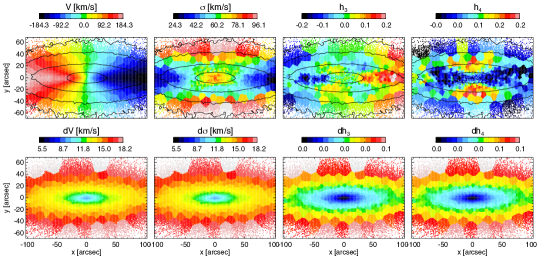
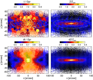
Figure 1: MUSE-like mock data created from the simulation Au-6, projected with inclination angle of $\vartheta=80^{o}$. The six columns from left to right are mean velocity $V$, velocity dispersion $\sigma$, GH coefficients $h_{3}$ and $h_{4}$, age and metallicity. The first row are perturbed data, the second row are errors ($dt$ and $dZ$ are $10\%$ of the original unperturbed data). The overplotted contours represent the surface mass density.

For real galaxies, the kinematic maps obtained from observations are usually light-weighted, In that case, we typically measure light-weighted age and metallicity maps, and use surface brightness as the tracer density for consistency. Orbits in the model should be interpreted as light-weighted. Here, however, the mock kinematics, age, and metallicity maps are mass-weighted so that we use surface mass density - rather than surface brightness - as the tracer density distribution. Therefore, the orbits in the model are mass-weighted. For method validation, mass-weighted or light-weighted data do not make any difference.

3 Method

In this section we describe how we fit the stellar kinematic maps as well as the age and metallicity maps with a population-orbit superposition method. The model will proceed as a two-step process: first, fitting the kinematics maps with a standard Schwarzschild’s orbit-superposition model to obtain the orbit weights; second, tagging the orbits with age and metallicities and fitting the age and metallicity maps, to obtain the best-fit age and metallicity of the orbits.

3.1 Schwarzschild method

The three main steps to build a Schwarzschild model are: 1) create a suitable model for the underlying gravitational potential; 2) calculate a representative library of orbits within the gravitational potential; and 3) find the combination of orbits (solve the orbit weights) that match the observed kinematic maps and luminosity/mass distribution of the tracers.

The gravitational potential is constructed by a combination of stellar mass distribution and dark matter halo. We de-project the surface brightness to 3D luminosity density by assuming a set of viewing angles ($\vartheta,\psi,\phi$). By multiplying the surface brightness by a stellar mass-to-light ratio, we obtain the intrinsic stellar mass density. Here for the mock galaxies, we actually use surface mass density, instead of surface brightness, to construct the gravitational potential. We still allow for a scale parameter $\alpha_{\rm star}$, which is analogous to a mass-to-light ratio, but with a true value of $1$, to be a free parameter.

A Multi-Gaussian Expansion (MGE) is used for modelling the surface density and de-projection to 3D density for the stellar component (Emsellem, Monnet & Bacon, 1994; Cappellari, 2002). We use the parameters describing intrinsic shapes ($q=Z/X$, $p=Y/X$, $u=\sigma_{\rm obs}/\sigma_{\rm intr}$) of the Gaussians, instead of the three viewing angles as free parameters. X, Y, Z are the intrinsic major, intermediate and long axis of the galaxy, $u$ is the ratio between $\sigma$ of observed long axis to the intrinsic long axis. For galaxies close to axisymmetric, we fix $u=0.9999$, while $p$ and $q$ are left free, thus triaxiality of the stellar component is still allowed. The dark matter is assumed to be a spherical NFW halo, with concentration $C$ fixed according to $M_{\rm 200}$ vs. $C$ correlation of Dutton & Macciò (2014).

In summary, we have four free parameters describing the gravitational potential: the scale parameter of stellar mass $\alpha_{\rm star}$ (comparable to a stellar mass-to-light ratio), intrinsic shape parameters $p$ and $q$, and dark matter virial mass $M_{\rm 200}$.

The method of orbit library sampling and model fitting follow exactly as described in Zhu et al. (2018b) and van den Bosch et al. (2008), which we do not repeat here. It should be emphasized that we do not fit $V$, $\sigma$ maps directly, but rather the LOSVD expanded in GH coefficients $h_{1}$, $h_{2}$, $h_{3}$ and $h_{4}$ to solve the orbit weights. However, we extract $V$ and $\sigma$ maps from the model at the end for direct comparison to the observational data. By exploring the free parameters describing the gravitational potential, we find the best-fitting model which reproduces the observed stellar kinematic maps and mass distribution.

We characterise the orbits with two parameters: time-averaged radius $r$ and circularity $\lambda_{z}$. Following Zhu et al. (2018b), $\lambda_{z}$ is defined as the angular momentum $L_{z}$ normalized by the maximum that is allowed by a circular orbit with the same binding energy. All quantities are taken as average of the particles sampled along the orbit over equal time interval. The stellar orbit distribution of a galaxy is described as the probability density distribution in the phase-space of $\lambda_{z}$ vs. $r$. Figure 2 illustrates the orbit distribution of a typical spiral galaxy. Darker color indicates higher probability; the total weight of the orbits has been normalized to unity.

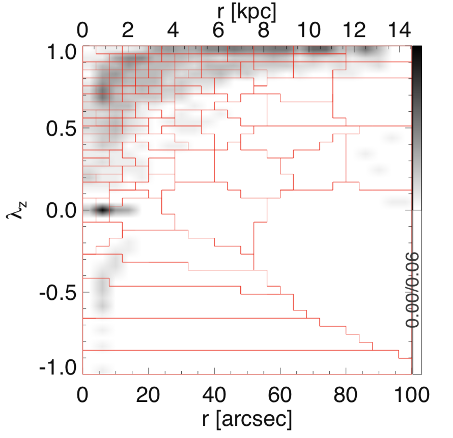
Figure 2: Probability density of stellar orbits in the phase space of circularity $\lambda_{z}$ versus time-averaged orbital radius $r$. Darker color indicates higher probability as indicated by the colorbar, and the total orbit weight has been normalized to unity. This galaxy has a large fraction of highly circular tube orbits with $\lambda_{z}\sim 1$ extending to large radius. In the inner regions, there are more tube orbits with significant random motions with $\lambda_{z}\sim 0.5$, some radial-motion dominated box orbits $\lambda_{z}\sim 0$ , and a small fraction of counter-rotating orbits with $\lambda_{z}<0$. The red polygons indicate the Voronoi binning scheme we have adopted in the phase-space, yielding $\sim 100$ orbit bundles, each with a minimum weight of 0.005.

The orbit library consists of a few thousand orbits, and a few hundred of them gain significant weights at the end. To reduce the noise in fitting age and metallicity maps, we perform a Voronoi binning in the phase-space $r$ vs. $\lambda_{z}$, and divide the orbits into $N_{\rm bundle}\sim 100$ bundles. Orbits with similar $r$ and $\lambda_{z}$ are included in the same bundle, to ensure each bundle has a minimum of orbit weight of 0.005. The resulting binning scheme is shown as the red polygons in Figure 2.

3.2 Tagging stellar orbits with stellar populations

The observed age map presents values of age, $t_{\rm obs}^{i}$, at each aperture $i$ on the observational plane, with a total number of $N_{\rm obs}$ apertures. Throughout the paper, one aperture indicates one spatial bin on the observational plane which may include a few pixels. After dividing the orbits into $N_{\rm bundle}$ bundles (Figure 2), we re-sample particles from these orbits in each bundle, with the number of particles proportional to their orbit weights. Then we add up all the particles sampled from each orbit bundle, project them to the observational plane, and calculate the mass $f_{k}^{i}$ (mass for mass-weighted and flux for light-weighted models) contributed by the orbital bundle $k$ at each aperture $i$.

This orbit bundle k, is tagged with a single value of age $t_{k}$. The average value of age in each aperture $i$ is a linear average of the $N_{\rm bundle}$ orbital bundles:

$$t_{\rm obs}^{i}=\Sigma_{k=1}^{N_{bundle}}t_{k}f_{k}^{i}/\Sigma_{k}f_{k}^{i},$$ (1)

for $i=1,...N_{\rm obs}$. Similarly, for metallicity:

$$Z_{\rm obs}^{i}=\Sigma_{k=1}^{N_{bundle}}Z_{k}f_{k}^{i}/\Sigma_{k}f_{k}^{i}.$$ (2)

We then solve for the values of $t_{k}$ and $Z_{k}$ using a Bayesian statistical analysis, which we will describe in detail in Section 3.4. As we will see, reproducing on-sky age and metallicity maps may be possible, however to reproduce them with the correctly correlated combinations of age and especially metallicity is non-trivial.

3.3 Age-metallicity correlation

We wish to adopt the most agnostic parameterization of the possible metallicity and age values for each orbit bundle. Unfortunately, a completely unconstrained age-metallicity parameter space results in poor recovery of the known 2D distribution on age vs. metallicity (see in section 4.3).

In order to provide a theoretically motivated link between age and metallicity which is flexible enough and unbiased for our purposes, we leverage the statistical chemical scaling relations presented in Leaman (2012), and model described by Oey (2000). These essentially map a galaxy’s chemical evolution into a parameter space that is: 1) self-similar across time and spatial scales for galaxies of different masses, and 2) is easily expressed in a robust statistical functional form (binomial).

The shape of galaxy age-metallicity relations and metallicity distribution functions show mass dependent behaviours (e.g. Kirby et al., 2013; Leaman, VandenBerg & Mendel, 2013). However Leaman (2012) identified that in linear metal fraction ($Z/Z_{\odot}$), all Local Group galaxies (in mass range of $M_{*}<10^{10}\,M_{\odot}$) exhibit metallicity distribution functions that are binomial in statistical form i.e., the variance $\sigma(Z)^{2}$, and mean $<Z>$ are tightly correlated, but the ratio is less than unity. Using a binomial chemical evolution model from Oey (2000), Leaman (2012) demonstrated that galaxies approximately evolve along the $\sigma(Z)^{2}-Z$ scaling relation. This provides a mass-independent, self-similar framework to link two quantities of interest: the spread in metals and the average metallicity of a galaxy or region of a galaxy.

To further link age to these two quantities we consider the binomial chemical evolution model of Oey (2000), which produces metallicity distribution functions with variance and mean:

$$\sigma(Z)^{2}=nQ(1-Q),\\ <Z>=nQ,\\$$ (3)

where $n$ represents the final number of star forming generations, and $Q$ represents the covering fraction of enrichment events within a generation. To make time explicit in the model, we consider that the gas reduction increment in the Oey (2000) model, $D=1-n\delta$, can be related through the gas fraction definition as:

$$\frac{M_{gas}}{M_{*}}=\frac{1-n\delta}{n\delta}.$$ (4)

From this we can express an approximate star formation law and relate it to $n$ in the binomial model as:

$$n=\frac{M_{*}}{\delta}=\frac{\int_{t}^{t_{H}}\epsilon SFR(\tau)d\tau}{SFR(t)},$$ (5)

where $t_{H}$ is the Hubble time and $t$ is when the last generation of SF happens. Following empirical and theoretical SF laws, we have introduced $\epsilon$ to allow for non-perfect conversion of gas to stars. This variable is often expressed as an inverse of the gas depletion time: $\epsilon=1/t_{\rm dep}$.

For a constant SFR, $n$ then becomes:

$$n=\frac{t_{H}-t}{t_{\rm dep}},$$ (6)

where $t_{H}-t$ is the length of time that all generations of star formation last in the galaxy. Combining this with the expressions for variance and mean Z in equation 3 we find:

$$\sigma(Z)^{2}=Z\left(1-\frac{Zt_{dep}}{t_{H}-t}\right).\\$$ (7)

This can then be re-expressed as a link between age, average metallicity and spread in metallicity:

$$t=t_{H}-t_{\rm dep}\frac{Z}{1-\sigma(Z)^{2}/Z}.$$ (8)

We can now use the equation 8 to set a mass-independent link between age and metallicity distributions. To further link these quantities and specify the metallicity spread in terms of average metallicity, we consider the observed statistical correlations present in metallicity distributions of Local Group dwarf to MW mass galaxies. Empirically, the observed relation between $\sigma(Z)$ and $Z$ from local group galaxies (Leaman, 2012):

$$\sigma(Z)^{2}=10^{a+b\log 10(Z)},$$ (9)

where $a=-0.689$ and $b=1.889$ shown as the black solid line in the top panel of Figure 3. As our priors are best expressed in natural log space, and considering $\ln{Z}$ of each population follows a Gaussian distribution, then a purely mathematical calculation yields

$$g(Z)\equiv\sigma(ln(Z))=\sqrt{\ln(1+\sigma(Z)^{2}/Z^{2})}.$$ (10)

Combined with equation 9, this yields for $g(Z)$ the black solid curve shown in the bottom panel of Figure Figure 3.

Setting $t_{H}=14$ Gyr and by substituting $\sigma(Z)^{2}$ from equation 9 into equation 8, we obtain a relation between average metallicity $Z$ and formation time $t$. This age-metallicity relation $Z(t|t_{\rm dep})$ still depends on depletion time $t_{\rm dep}$. As shown in Figure 4, $Z(t)$ is steeper with smaller $t_{\rm dep}$, and shallower with larger $t_{\rm dep}$. Actually, $t_{\rm dep}$ will likely be different for different regions in a galaxy with complicated star formation history. The dots overplotted in Figure 4 are the observed age $t_{\rm obs}$ and metallicity $Z_{\rm obs}$ (Au-6 $\vartheta=80^{o}$) colored by their elliptical radius $R_{\rm ellp}=\sqrt{x^{2}+y^{2}/(q_{\rm obs})^{2}}$ on the observational plane, where $q_{\rm obs}$ is observed flattening of the galaxy. There is almost a linear correlation between $t_{\rm dep}$ indicated by ($t_{\rm obs}$, $Z_{\rm obs}$) and radius $R_{\rm ellp}$ (also see figure 15 in the appendix). The star formation in a galaxy is consistent with smaller $t_{\rm dep}$ at small radii, and larger $t_{\rm dep}$ at large radii. We note that the range of depletion times is consistent with those found for a wide range of galaxy masses, regions - including at larger redshifts (c.f. Bigiel et al., 2011).

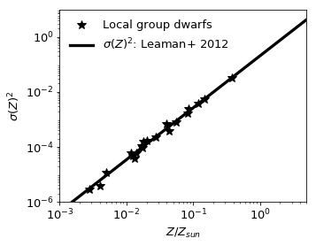
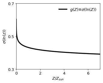
Figure 3: Top: , the relation of metallicity spread $\sigma(Z)$ vs. $Z$, the black stars are local group dwarf galaxies from (Leaman, 2012), the black curve (labeled as a) is fitting to these data points (equation 9). Bottom: $\sigma(ln(z))$ vs. $Z$ converted from the curve in the top based on equation 10.

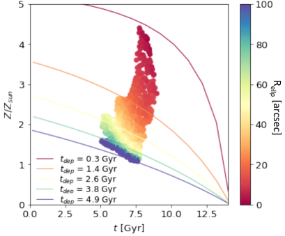
Figure 4: The age-metallicity relation $Z(t|t_{\rm dep})$ derived with combination of equation 8 and equation 9. The solid curves with different colors are $Z(t)$ by choosing different $t_{\rm dep}$ as labeled. The dots are the observed age $t_{\rm obs}$ and metallicity $Z_{\rm obs}$ (Au-6 $\vartheta=80^{o}$) colored by their elliptical radius $R_{\rm ellp}$ on the observational plane.

3.4 Bayesian analysis

We use Bayesian statistical analysis (Python package pymc3) to obtain age ($t_{k}$) and metallicity ($Z_{k}$) of the orbital bundles.

3.4.1 Fit to age map

We first fit the age map following equation 1. In pymc3, we can specify a prior for each parameter as a distribution. We adopt a bounded normal distribution:

$$f(t_{k}|\mu_{k},\sigma_{k})=\sqrt{\frac{1}{2\pi\sigma_{k}^{2}}}\exp{-\frac{(t_{k}-\mu_{k})^{2}}{2\sigma_{k}^{2}}}$$ (11)

for $t_{k}$ with lower and upper boundary of 0 and 14 Gyr, we set $\mu_{k}$ and $\sigma_{k}$ as follows:

$$\mu_{k}={\rm Randn}(<t_{\rm obs}>,2\sigma(t_{\rm obs}))\hskip 90.00014pt$$ (12)

$$\sigma_{k}=2\sigma(t_{\rm obs}),$$ (13)

where $<t_{\rm obs}>$ and $\sigma(t_{\rm obs})$ indicate average and standard deviation of age from the observational age map. Note that ${\rm Randn}(a,b)$ means a random number generated from normal distribution with center $a$ and dispersion $b$, the above priors are uniform for all the orbital bundles.

Once the priors are specified, we start the Markov Chain Monte Carlo (MCMC) analysis by adopting a student T distribution $t_{\nu}(x|\mu,\sigma)$ for the posterior likelihoods. The chain is initialized with the method ‘ADVI’-Automatic Differentiation Variational Inference-with 200000 draws, and we run 2000 steps. We take the average and standard deviation of the last 500 steps as mean and $1\sigma$ uncertainties of $t_{k}$. The last 500 steps will also be used for smoothing the overall age distribution of the galaxy obtained by our model.

In general, we expect stellar kinematics to be systematically correlated with stellar age, because stars on dynamical hot orbits are systematically older than stars on near-circular orbits (Trayford et al., 2018). From our experience, with the above priors for $t_{k}$, it is not easy to perfectly recover the correlation between stellar age $t$ and orbits’ circularity $\lambda_{z}$, especially for the face-on galaxies (see Section 4.4). The results could be improved by fitting a linear relation $t=t_{0}+p\lambda_{z}\,(\lambda_{z}\geq 0.0)$ to the $t(\lambda_{z})$ relation of the first model. Then for the second model iteration, we set the $\mu_{k}$ and $\sigma_{k}$ of the Gaussian priors as:

$$\mu_{k}={\rm Randn}(t_{0}+p\lambda_{z,k},2\sigma(t_{\rm obs})-|p|/2)\hskip 10.00002pt(\lambda_{z,k}\geq 0.0)\\ \hskip 10.00002pt=t_{0}\hskip 153.00026pt(\lambda_{z,k}<0.0)\\$$ (14)

$$\sigma_{k}=2\sigma(t_{\rm obs}).$$ (15)

In this case, the standard deviation of $\mu_{k}$s are still $\sim 2\sigma(t_{\rm obs})$, similar to the previous prior. We perform the Bayesian analysis again with the new priors. This iterative process could be repeated more than once, but we found the results already converged after the first iteration. We stress this is only an iterative refinement on the choices of priors, not a prescribed link between age and circularity directly.

3.4.2 Fit to metallicity map

After we have obtained ages of the orbital bundles, We then fit the metallicity map following equation 2. Metallicity expressed in linear unit $Z/Z_{\rm sun}$ is adopted in our analysis. We use a bounded lognormal distribution as prior of metallicity $Z_{k}$ of each orbital bundle:

$$f(Z_{k}|\mu_{k},\sigma_{k})=\frac{1}{Z_{k}}\sqrt{\frac{1}{2\pi\sigma_{k}^{2}}}\exp{-\frac{(\ln{Z_{k}}-\mu_{k})^{2}}{2\sigma_{k}^{2}}},$$ (16)

with lower and upper boundary of 0 and 10. We first start with $\mu_{k}$ and $\sigma_{k}$ of the lognormal distribution as follows:

$$\mu_{k}=\ln({\rm Randn}(<Z_{\rm obs}>,\sigma(Z_{\rm obs})))$$ (17)

$$\sigma_{k}=\sigma(Z_{\rm obs}),$$ (18)

where $<Z_{\rm obs}>$ and $\sigma(Z_{\rm obs})$ are the average value and standard deviation of metallicity from the observational metallicity map. Then we perform Bayesian analysis similar to the fitting of age map. We take the average and standard deviation of the last 500 steps of the MCMC chain as mean and $1\sigma$ error of $\ln(Z_{k})$, the last 500 steps are also used for smoothing the overall metallicity distribution of the galaxy obtained by our model.

The above uniform priors for $Z_{k}$ lead to a poor recovery of the age-metallicity distribution. To this end, we use the age-metallicity relation derived in Section 3.3 to give more reasonable priors for $Z_{k}$, with age of each orbit $t_{k}$ already obtained. We adopt again the bounded lognormal distribution, but now with $\mu_{k}$ and $\sigma_{k}$ given by:

$$\mu_{k}=\ln(Z(t_{k}|t_{\rm dep}(r_{k})))$$ (19)

$$\sigma_{k}=g(\mu_{k}).$$ (20)

We let the depletion time locally vary as a function of radius $r_{k}$ (which traces mass density), and refer the reader to Appendix A for details.

In order to understand how the different priors on $t_{k}$ and $Z_{k}$ affect our results, We perform two model fits to age and metallicity maps - an unconstrained version, and one with the above mentioned priors. These are summarized in Table 2. The model results from these different priors are marked as R1 and R2 respectively, throughout the paper.

Table 2: The priors for the Bayesian fitting to age and metallicity maps. We have $\sim 100$ orbital bundles in the model, $k$ indicates any of these. We take a bounded normal distribution as prior for $t_{k}$ (equation 11), a bounded lognormal distribution for $Z_{k}$ (equation 16), with the mean $\mu_{k}$ and dispersion $\sigma_{k}$ specified differently for the two rounds of model fitting: R1, R2. When fitting to age, for Model R1, we use uniform priors for $t_{k}$, and for Model R2 we use a relation $t_{k}=t_{0}+p\lambda_{z,k}$ fitted from the result of model R1. When fitting to metallicity, for Model R1 we use uniform priors for $Z_{k}$, while for Model R2 we use the age-metallicity-metallicity spread relation $Z(t|t_{\rm dep})$ (Figure 4), $g(Z)$ (Figure 3) (see Section 3.3).

Model	prior for age $t_{k}$
	${\rm Norm}(t_{k}|\mu_{k},\sigma_{k})$
R1	$\mu_{k}={\rm Randn}(<t_{\rm obs}>,2\sigma(t_{\rm obs}))$
	$\sigma_{k}=2\sigma(t_{\rm obs})$
R2	$\mu_{k}={\rm Randn}(t_{0}+p\lambda_{z,k},2\sigma(t_{\rm obs}-|p|/2))$
	$\sigma_{k}=2\sigma(t_{\rm obs})$
Model	prior for metallicity $Z_{k}$
	${\rm LogNorm}(Z_{k}|\mu_{k},\sigma_{k})$
R1	$\mu_{k}=\ln({\rm Randn}(<Z_{\rm obs}>,\sigma(Z_{\rm obs})))$
	$\sigma_{k}=\sigma(Z_{\rm obs})$
R2	$\mu_{k}=\ln(Z(t_{k}|t_{\rm dep}(r_{k})))$
	$\sigma_{k}=g(\mu_{k})$

4 Results on stellar orbit and population distributions

In this section, we describe how the models match the intrinsic orbit distribution, age-metallicity distribution and age-circularity correlation with the nine MUSE-like mock data created from Auriga simulation. For illustration of model fitting and some results, we do not show all nine galaxies but just Au-6 $\vartheta=80^{o}$. We refer the reader to Appendix B for results for the other galaxies.

4.1 Best-fitting model

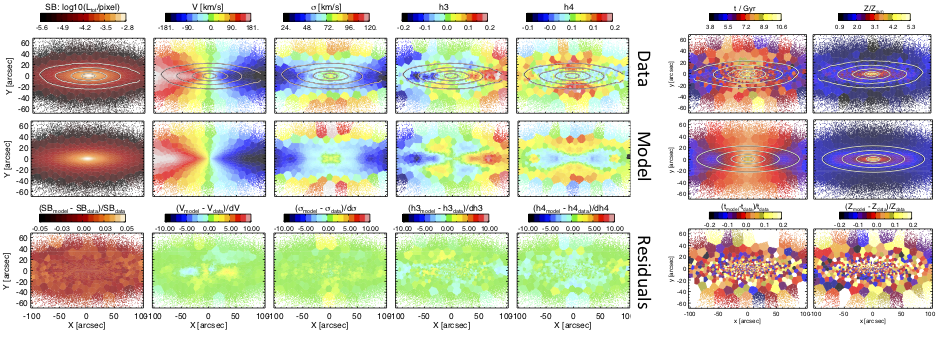
Figure 5: The best-fitting model. The columns are surface mass density, mean velocity $V$, velocity dispersion $\sigma$, GH coefficient $h_{3}$, $h_{4}$, age and metallicity $Z$. The first row are observational data, the second row are from the best-fitting model, and the third row are residuals.

A best-fitting model of the mock data from Au-6 with $\vartheta=80^{o}$ is shown in Figure 5. From left to right, the columns are surface mass density, mean velocity, velocity dispersion, $h_{3}$, $h_{4}$, age ($t$) and metallicity ($Z$). The first row is the data, the second row is reproduced by the best-fitting model and the third is residual. The model matches the kinematic maps, age and metallicity maps well. For just the projected on-sky maps, we see that the models with different priors (R1, R2) fit the age and metallicity maps equally well.

In summary, up to this point we have obtained an orbit-superposition model, with the orbit weights solved by matching the stellar mass distribution and kinematic maps. Here we further divided the orbits into $\sim 100$ bundles, and obtained the age and metallicity of these bundles by fitting the age and metallicity maps. By taking a Bayesian statistical analysis, we obtained the mean value $t_{k}$ and $Z_{k}$ of each bundle $k$, as well as their uncertainties $\sigma(t_{k})$, $\sigma(Z_{k})$.

4.2 Stellar orbit distribution

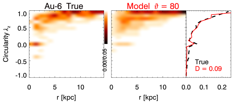
Figure 6: The stellar orbit distribution described as probability density of orbits in the phase space of $\lambda_{z}$ vs. $r$, for Au-6. The left panel is the true stellar orbit distributions from simulations. The second is the distribution of orbits in our best-fitting model for mock data with $\vartheta=80^{o}$. The right panel is comparison of marginalized $\lambda_{z}$ distribution between true and model. Similar figures for the other galaxies are included in the appendix Figure 16.

We first check how well the orbit distribution in our model matches the true distribution from the simulation. The real gravitational potential and 6D phase-space information of particles are known in the simulation. Thus we know the instantaneous circularity $\lambda_{z}$ of each particle (Gómez et al., 2017), which does not necessarily conserve $\lambda_{z}$ when orbiting in the potential, especially for those particles on radial/box orbits with $\lambda_{z}\sim 0$. To obtain the orbits’ circularity, in principle, we have to freeze the potential, integrate the particle orbits in the potential, and calculate the average values along the orbits. Here for simplicity, we use a single snapshot and select those particles that are close in energy, $E$, angular momentum, $L_{z}$ and the total angular momentum amplitude, $|L|$. Under the assumption that these particles are on the same orbit in a near axisymmetric system, we then compute the corresponding averages of radius $r$ and circularity $\lambda_{z}$ of these particles, which are taken as the orbit’s $r$ and $\lambda_{z}$. The stellar orbit distribution of one galaxy is then presented as the probability density distribution of all these orbits in the phase space of $r$ vs. $\lambda_{z}$, which is shown in the left panel of Figure 6 for Au-6.

In our model, we calculate orbit’s circularity and time-averaged radius from the particles sampled from the orbit with equal time interval. The middle panel of Figure 6 shows the the distribution of orbits in our best-fitting model for mock data Au-6 $\vartheta=80^{o}$.

Our model matches the major features in the phase-space of $r$ vs. $\lambda_{z}$ as the true orbit distribution from the simulations. For the case of Au-6 $\vartheta=80^{o}$ we show here, counter-rotating (CR) orbits contribute a small fraction in the simulation, and our model underestimate CR orbits by $\sim 50\%$. The right sub-panel is the marginalized $\lambda_{z}$ distribution. The black dashed curves is the true distributions; red solid curves represent that from our model. We did a 1D KS test to check how well the $\lambda_{z}$ distribution recovered by our model match the true distribution from simulation. The D-statistics $D$ is the maximum deviation from the accumulated curves of two distributions. We obtained $D=0.09$ here for the $\lambda_{z}$ distribution A similar comparison for Au-5, Au-6, Au-23 with inclination angles of $\vartheta=40^{o},60^{o},80^{o}$ are shown in the appendix in Figure 16.

4.3 Age-metallicity distribution

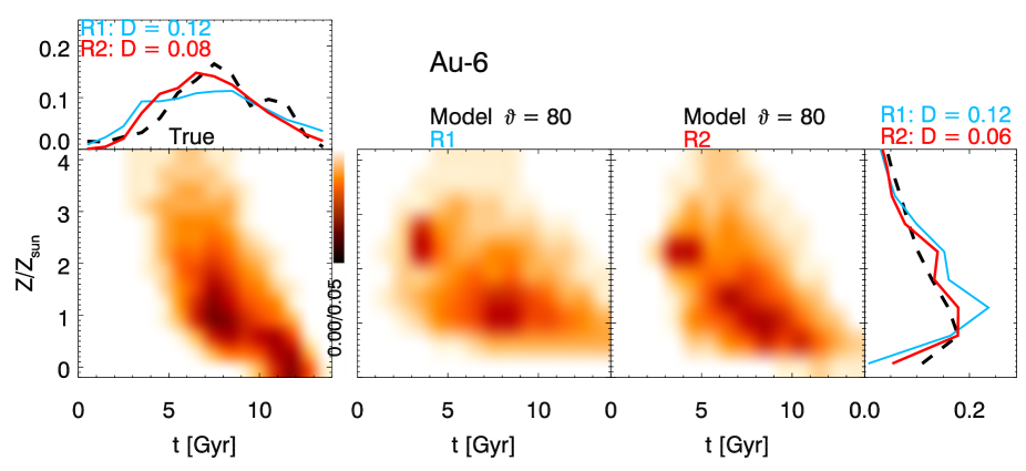
Figure 7: The intrinsic age-metallicity distribution for Au-6 $\vartheta=80^{o}$. The left panel is the true distribution in stellar age $t$ vs. metallicity $Z$ of particles of the simulation. The rest panels are obtained by our model constrained by mock data Au-6 $\vartheta=80^{o}$ with priors R1 and R2 from left to right. The probability contours of our models are smoothed by the last 500 steps of MCMC chains of $t_{k}$ and $Z_{k}$ from the Bayesian analysis. The upper subpanel is the marginalized age distribution and the right sub-panel is the marginalized metallicity distribution. The black dashed curve is the true, red, blue solid curves represent that from model with priors R1, R2, respectively. The D-statistics $D$ calculated from KS test comparing 1D age/metallicity distribution from our model to the true age/metallicity distribution are labeled.

Age and metallicity maps projected on-sky can be reproduced with many degenerate combinations of age-metallicity distributions of the stars. However, not all combinations may be physical, nor match the intrinsic age vs. metallicity distribution of the simulated galaxy. Here we check how the age and metallicity distribution of orbits in our models match the intrinsic distribution of particles in these simulations.

In Figure 7, we show the probability density distribution of particles/orbits in age ($t$) vs. metallicity ($Z/Z_{\odot}$), from the simulations and from our model of Au-6 $\vartheta=80^{o}$. The first panel labeled with ‘True’ shows the true distribution on Age vs. $Z$ of particles in the simulation. The following panels are those obtained by our model for mock data $\vartheta=80^{o}$ but with prior R1, R2 from left to right. The probability contours are smoothed by the last 500 steps of MCMC chains of $t_{k}$ and $Z_{k}$ from the Bayesian analysis.

The upper sub-panel for each halo is the marginalized age distribution and the right sub-panel is the marginalized metallicity distribution. The black dashed curves are the true distributions; red, blue solid curves represent those from models with prior R1 and R2, respectively. From a 1D KS test, we obtained $D=0.12,0.08$ for age distribution and $D=0.12,0.06$ for metallicity distribution, for models with prior R1 and R2, respectively. Both intrinsic age and metallicity distributions are recovered better with model R2 than R1.

In the true distribution, most stars follow a relation with older stars that are more metal-poor. Model R1 hardly recovers this relation (Figure 7), missing a significant fraction in mass of sub-solar metallicity stars, and showing roughly uncorrelated distributions of constant metallicity groupings over a wide range in age. The recovery of age-metallicity relation significantly improved with model R2, especially for more face-on galaxies (see Figure 17 and Figure 18).

4.4 Age-circularity correlation

In this Section, we study the correlation of stellar orbit circularity and ages in the simulation, and check how well the correlation can be recovered by our models.

The intrinsic probability density distribution of orbits on age $t$ vs. circularity $\lambda_{z}$ for simulation Au-6 is shown in the left panel of Figure 8. darker color indicates higher probability density. In the simulation, there is a correlation between stellar age and orbits’ circularity: highly circular orbits are systematically younger, and radial-motion dominated orbits are older. We calculate the average age of orbits as a function of $\lambda_{z}$ by binning on $\lambda_{z}$ (the magenta dashed curve) and average $\lambda_{z}$ as a function of age by binning on age $t$ (the green dashed curve).

The orbit distribution on age vs. circularity obtained by our models with Au-6 $\vartheta=80^{o}$ are shown in the following panels, for model R1 and R2 respectively. In each panel, the probability contours represent the distribution that is derived from the last 500 steps of MCMC chain of $t_{k}$ from the Bayesian analysis. The magenta triangles are average age as function of $\lambda_{z}$ from the model. The magenta solid line ($t=t_{0}+p\lambda_{z}$) is a linear fit to the triangles, which from model R1 is used as prior of age $t_{k}$ for model R2 when fitting to age map. The green diamonds are average $\lambda_{z}$ as a function of age by binning on age from the model.

Our models generally match the $t\sim\lambda_{z}$ correlation from the simulation, model R2 matches it better than R1 for Au-6 $\vartheta=80^{o}$; the improvement of R2 comparing to R1 is more significant for more face-on galaxies (see Figure 19, Figure 20). The results in following sections are based on Model R2 if not otherwise specified.

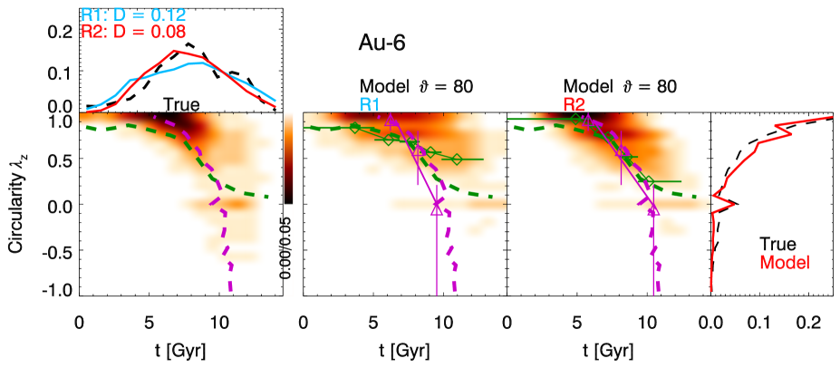
Figure 8: The intrinsic correlation of age vs circularity, for Au-6 and those from our models with mock data $\vartheta=80^{o}$. The first one is the true distributions of the particles from simulation, darker color indicates higher probability density, the magenta dashed curve is average age $t$ as a function of $\lambda_{z}$, while the green dashed curve is average $\lambda_{z}$ as a function of age $t$ from the simulation. The following panels are obtained by model R1 and R2 respectively. In each panel, the magenta triangles are average age as a function of $\lambda_{z}$ for the corresponding panel, the magenta solid line is a linear fit ($t=t_{0}+p\lambda_{z}$) to the triangles. The magenta solid line from model R1 is used as priors of ages $t_{k}$ in model R2. Similarly, the green diamonds represent average $\lambda_{z}$ as a function of age $t$ for the model. Model R2 matches the true relations in the simulation better than model R1.

5 Orbital decomposition

To further quantify the correlation between the orbits’ dynamical properties and stellar populations, we decompose galaxies (c.f., Zhu et al., 2018b) by dividing the orbits into cold ($\lambda_{z}\geq 0.8$), warm ($0.25\leq\lambda_{z}<0.8$), hot ($|\lambda_{z}|<0.25$), and counter-rotating (CR, $\lambda_{z}<-0.25$) components. We emphasis that the separation of cold, warm, hot+CR components is just for proof of concept. For real galaxies, we may adjust the component separation case by case.

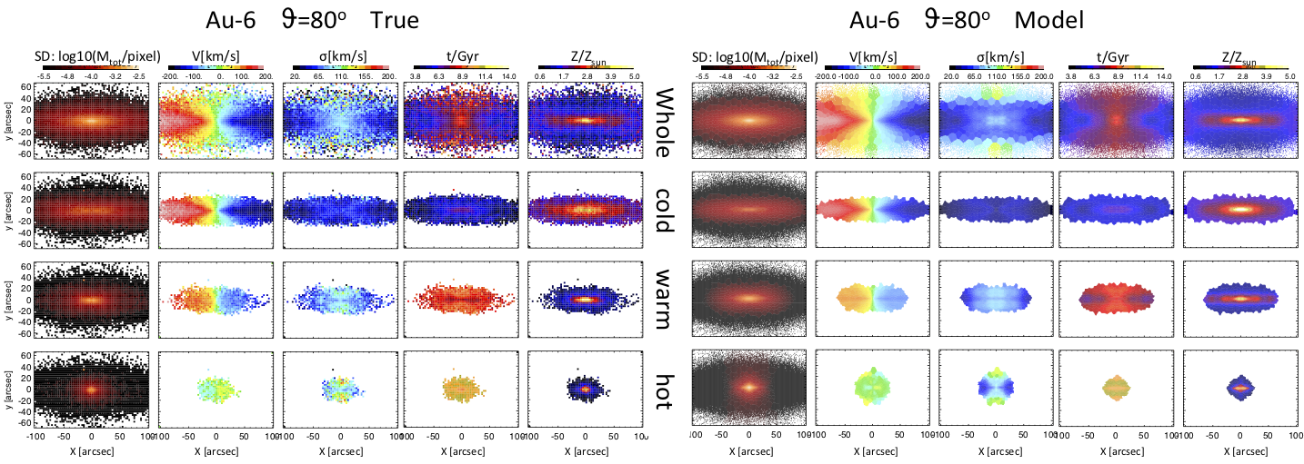
Figure 9: Surface mass density, age, and metallicity maps of the whole galaxy, cold, warm, and hot + CR component (from top to bottom) of Au-6 $\vartheta=80^{o}$. The left panels are constructed by particles in the simulation, the right panels are constructed by orbital bundles in our model constrained by mock data with $\vartheta=80^{o}$. The galaxy is at a distance of 30 Mpc, $1^{\prime\prime}=145\,{\rm pc}$.

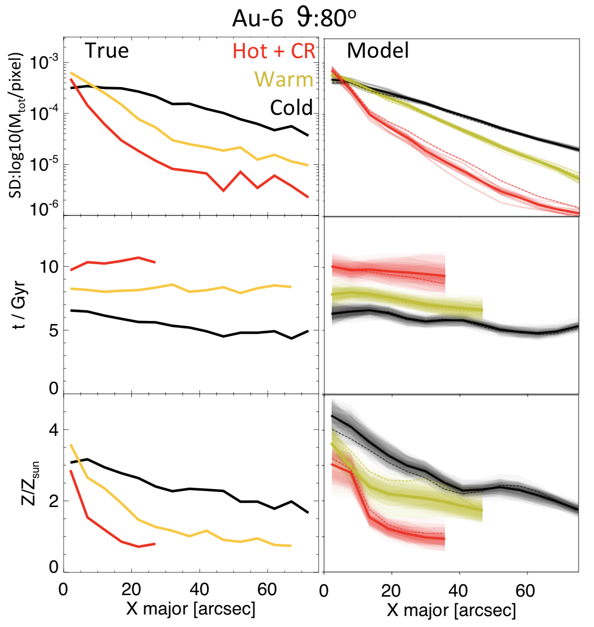
Figure 10: Surface mass density, age, and metallicity profiles along major axis ($1^{\prime\prime}=145\,{\rm pc}$) of the cold (black), warm (warm), and hot + CR (red) component of Au-6 $\vartheta=80^{o}$. The left panels are constructed by particles in the simulation. The right panels are those constructed by orbital bundles in our model constrained by mock data with $\vartheta=80^{o}$, the shadow regions indicate $1\,\sigma$ uncertainty of our models, the solid thick curves are average of models within $1\,\sigma$, and the dashed thin curves are the best-fitting one.

We rebuild the 3D structure for each of the cold, warm, hot + CR components, by particles in simulations and orbits in models. Then we project the 3D structures, here with the same inclination angle as the galaxy was observed, to the observational plane, thus obtaining surface density (SD), mean velocity and velocity dispersion, age, and metallicity maps for each component. In Figure 9, we compare these maps from the simulation Au-6 (left) to those recovered from our model with mock data Au-6 $\vartheta=80^{o}$ (right).

Our model generally reproduces the morphology, kinematics, age and metallicity maps of the different components: the cold component is a thin disk, spatially extended, fast rotating with small velocity dispersion, young and metal-rich; the warm component is thicker and less radially extended, with weaker rotation and higher velocity dispersion, older and metal-poorer; and the hot + CR component is spheroidal and spatially concentrated, with almost no rotation and high velocity dispersion, with oldest and most metal-poor stellar populations. The 2D maps, both along the major and minor axis, of each component are visually well recovered by our model.

For a quantitatively comparison, we show in Figure 10 the radial profiles (along the major axis) of the SD, age and metallicity for the cold, warm, hot + CR component, obtained from the simulation (left) and from our model (right). The three components are plotted as black, yellow and red. In the right panels, we show not only the best-fitting model, but all the models within $1\,\sigma$ uncertainty when fitting to kinematics (Zhu et al., 2018b). The shadow areas indicate the scatter of these models within $1\,\sigma$ uncertainty, the solid thick curves are corresponding averages and the thin dashed curves are the best-fitting one.

The simulation shows an increase in stellar age from cold to hot orbits, with little change in that behaviour with galactocentric distance; there is only a shallow negative gradient for the cold disk from inner to out regions. Our models generally reproduce this behaviour. An implication of this is that for the galaxy as a whole, the projected age gradient is a result of different dynamical components super-imposed: the old-hot component dominates in the centre and a young-cold component dominates in the outer regions.

The three components have similar metallicity ($Z/Z_{\rm sun}$) at the center, with a strong negative metallicity gradient in the hot+CR component, and the gradient becomes weaker from hot+CR, warm to cold component. Our models generally match the metallicity gradients for warm and hot+CR component, but over-estimate the metallicity of cold component in the inner region, thus resulting in a too strong metallicity gradient for the cold component.

A similar decomposition is performed for all galaxies. For edge-on galaxies ($\vartheta=80^{o}$), the age and metallicity profiles of three components are recovered similarly well for Au-5, Au-6 and Au-23 (see figure 21, figure 22). Age and metallicity profiles of each component are recovered less well in more face-on galaxies.

6 Global Age-dispersion relation

The stellar age vs. vertical velocity dispersion $\sigma_{z}$ relation is widely used for resolved systems to study the dynamical heating processes (e.g., Leaman et al., 2017). Here, we extract similar relations for external galaxies based on our model to galaxies with integrated-light data. Application of a similar approach to NGC 3115 has provided a $t\sim\sigma_{z}$ relation of this galaxy (Poci et al., 2019). Here we check how reliable the global (not disk alone) $t\sim\sigma_{z}$ relation can be recovered.

We can construct $t\sim\sigma_{z}$ relations by separating the galaxies into multiple components in two ways based on Figure 8, by applying a cut either on circularity $\lambda_{z}$, or on stellar age of the orbits in our model.

First we follow the separating on circularity $\lambda_{z}$ as we did in last section, to separate the simulation/model into cold, warm, hot+CR components, then we calculate the average age and $\sigma_{z}$ of each component. In Figure 12, we show the resulting $t\sim\sigma_{z}$ relation in these simulations and how our model recovered it. The three panels are for Au-5, Au-6, Au-23, respectively. In each panel, the black asterisks are the true ages and velocity dispersions $\sigma_{z}$ of each component from the simulation. There are strong age vs. $\sigma_{z}$ correlation in these three Auriga simulations; cold components have small $\sigma_{z}$ and are younger, while hot components have larger $\sigma_{z}$ and are older.

The red, blue, and purple diamonds represent those calculated from our models for galaxies with $\vartheta=80^{o},60^{o},40^{o}$, respectively. For all three simulations, our models match the average age of each orbital component well, thus also the $t\sim\sigma_{z}$ correlation. There are slightly larger offsets for the face-on galaxies ($\vartheta=40^{o}$), but they still generally match the trend. Our method works better for Au-5 and Au-23, in which the intrinsic age-$\sigma_{z}$ correlations are steeper, than Au-6, in which the correlation is shallower.

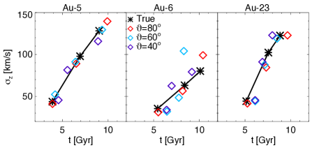
Figure 11: The global age $t$ vs. dispersion $\sigma_{z}$ relation. The three panels are for Au-5, Au-6, Au-23, respectively. we separate each galaxy to be cold, warm, hot+CR components based on the orbits’ circularity $\lambda_{z}$, and calculate average age and dispersion $\sigma_{z}$ for each component. In each panel, the black asterisks are the true values calculated from the simulations, dispersion increases with age from cold, warm to hot component, the solid black curve just connects the asterisks. The red, blue, and purple diamonds represent those calculated from our models for galaxies with $\vartheta=80^{o},60^{o},40^{o}$, respectively.

As local observations have traditionally computed the velocity dispersion of stars in similar age bins, we also separate the galaxy by applying cuts on stellar age, with equal mass in each bin. We use 10 age bins for the simulation, and 5 age bins for the models, and calculate average age and dispersion in each bin. In this way, it can be compared to similar observed vertical dispersion of galaxies at high redshift. The resulting $t\sim\sigma_{z}$ relation is shown in Figure 12.

By binning along stellar age, our models still recover the $t\sim\sigma_{z}$ relation reasonably well for edge-on galaxies. It is recovered less well for face-on galaxies, for which $\sigma_{z}$ of old populations are under-estimated by our model. This is likely due to the relative large uncertainty of age of each orbital bundle. Some cold orbits could get old ages, and so contaminate the old populations and lead to an under-estimation of $\sigma_{z}$.

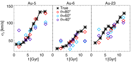
Figure 12: The global age $t$ vs. dispersion $\sigma_{z}$ relation. Similar to Figure 11, but by separating the simulation/model in to equal mass bins according to stellar age. We separate the simulation into 10 age bins, and model into 5 age bins.

7 Discussion

We have shown that our population-orbit superposition methods work well in recovering the intrinsic stellar orbit distributions and stellar population distributions of external galaxies. This method could be widely applied to nearby galaxies with IFU observations, making it possible to separate structures in external galaxies from a combination of stellar kinematics and stellar chemical properties, thus bridging the gap between the Milky Way and external galaxies.

The current method works well in a few important aspects, but also as we have shown, the interpretation of some results need to be taken with caution as it does not work equally well for all projections. Here we discuss in detail some limitations and how to improve it in the future.

7.1 Features of bars

We do no have a bar structure explicitly in the model. While Auriga galaxies are strongly barred. The bar regions of these galaxies are filled by mostly warm orbits with similar circularity in our model as the resonant orbits supporting the real bar in the simulation. Bars generally have similar stellar age as the disks, but are metal richer. We take Au-23 $\vartheta=40^{o}$ shown in Figure 13 as an example. The first row shows the mock data of age and metallicity maps with contours showing the real surface mass density. The second row is our best-fit to the data with contours showing surface mass density in our model. The bar is not a prominent feature in the age map, but much more obvious in the metallicity map. Based on the orbital constructions in our model, we do not have the ability to match the bar structure in the metallicity map. This could directly lead to a bias in the recovered metallicity for different orbital components.

For edge-on cases, the structure in metallicity caused by the bar could be roughly matched by assigning different metallicities to the corresponding warm orbits, thus our model can still work on recovering metallicities of cold, warm, hot+CR components. This is not the case for face-on projections. Including a bar explicitly in our Schwarzschild model in the future, as attempted in other studies (Vasiliev & Valluri, 2019), will certainty lead to improving recovery of metallicities of different structures in barred galaxies. In such a model, we may need a third parameter to characterise orbits, besides radius $r$ and circularity $\lambda_{z}$. Then orbit bundles divided on a 3D phase-space rather than 2D $r\sim\lambda_{z}$ plane might be used for tagging age and metallicities.

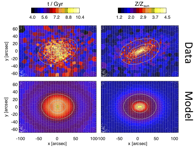
Figure 13: The best-fitting model of age (left) and metallicity (right) maps of Au-23 $\vartheta=40^{o}$. The first row is the mock data, a bar-like structure is not obvious in age map, but significant in metallicity, the contours over-plotted illustrate the real surface mass density of the galaxy which has a strong barred structure. The second row is our model fitted age and metallicity maps, the over-plotted contours illustrate the surface mass density of our model.

7.2 Beyond single age and metallicity per orbit

We tag a single value of age and metallicity to each orbit bundle divided in the 2D $r\sim\lambda_{z}$ plane, while each orbit bundle should have a distribution of age and metallicities. A consequence of this is the most-poor end of the metallicity distribution is difficult to match completely (See Figure 7 and Figure 18). This can be due to two effects which we explain below.

In the left panel of Figure 14, the contours are probability density distribution in age vs. metallicity of particles in the simulation. We divide the particles into different orbital bundles on $r\sim\lambda_{z}$, each diamond represent average age and metallicity of an orbit bundle. As can be seen, the age and metallicity distributions of the orbit bundles are narrower than those of true distribution of particles. There are rarely orbit bundles with average $Z/Z_{\rm sun}<0.5$ - even in the simulation. Thus it is expected that when assigning a single value of age and metallicity to each orbital bundle, our model will also show a narrow distribution in age and metallicity (even smoothing over the last samples of our pymc3 process).

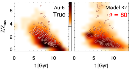
Figure 14: The intrinsic age-metallicity distribution for Au-6 $\vartheta=80^{o}$. In the left panel, the contours represent the probability density distribution of particles in the simulation, the diamonds represent age vs. metallocity of orbital bundles, which we obtained by dividing the particles based on 2D $r\sim\lambda_{z}$ plane. In the right panel, the diamonds are age vs. metallicity of orbital bundles in our model, the contours are smoothed by results of the last 500 steps of the pymc3 process.

A second, related aspect, is that our model is reproducing on-sky projected age and metallicity maps. For any projection, even at the high spatial resolution of modern MUSE observations, such spatial binning results in a significant loss in information when compared to the true particle age and metallicities. Further work looking at optimal reconstruction of true particle distributions from binned maps and observational estimates of line-of-sight metallicity and age distributions per pixel will provide help in this front. Technically, it is not difficult to impose an age and metallicity distribution to each orbital bundle. However, the distribution is fully unconstrained by our current data, which are only light/mass weighted age and metallicity maps averaged along line-of-sight. If we want to constrain the age and metallicity distributions of each orbital bundle, we will need line-of-sight age and metallicity distribution from observation, which we still need to further investigate from the observational side.

We find that the method works better for edge-on than face-on galaxies in a few aspects: recovering the general age vs. circularity correlation, the detailed age and metallicity profiles of different dynamical components, and the $t\sim\sigma_{z}$ relation. Apart from the presence of bars, age and metallicity information of different structures, e.g, thin/thick disks and bulge, are revealed in the edge-on age/metallicity maps, while blended in face-on projected data. The ability of recovering those properties for face-on galaxies could also improve if we can use line-of-sight age/metallicity distribution from observations as model constraints.

8 Summary

We present a population-orbit superposition method in this paper by tagging age and metallicity to orbits in the Schwarzschild model and requiring it to fit the observed luminosity/mass distribution, as well as stellar kinematics, age and metallicity maps. We validate the method by testing against mock data created from simulations. We take three simulations from Auriga, and project each simulation with three different inclination angles $\vartheta=80^{o},60^{o},40^{o}$. With each projection, we create a set of mock data with MUSE-like data quality, including surface mass density, stellar kinematics, age and metallicity maps. Thus, we have nine mock datasets in total, each is taken as an independent observed galaxy, to which we apply our method.

The mock data is fitted well by our model with no difficulty except for the barred features in face-on galaxies. To reproduce correct relations between age and metallicity, we found a physically motivated chemical evolution prescription for the priors significantly improved the results. To evaluate the method’s ability of recovering galaxies’ intrinsic properties, we compare these properties from our models to those from simulations:

• Our models can generally and equally well recover the stellar orbit distribution in the phase-space of circularity $\lambda_{z}$ vs. radius $r$ for galaxies with different viewing angles.

• The intrinsic stellar population distribution in age $t$ vs. metallicity $Z$ is hard to fully recover. We derived a theoretically motivated link between age, mean metallicity and metallicity spread, which we impose as priors when fitting metallicity maps. This link improved our recovery of age-metallicity correlations, and the marginalized metallicity distributions.

• Our method works well in recovering the age-circularity correlation for edge-on galaxies, but less well for more face-on galaxies. An iterative fitting by updating the priors for age based on an initial fit helps improving the results, especially for face-on galaxies.

• To further check the method’s ability on recovering intrinsic properties of different galaxy structures: we decompose galaxies into cold ($\lambda_{z}>0.8$), warm ($0.25<\lambda_{z}<0.8$), hot + CR ($\lambda_{z}<0.25$) components. We then rebuild the surface density, mean velocity, velocity dispersion, age and metallicity maps of each component. By comparing with those constructed from the simulation, we find these maps of each component are quantitatively well recovered by our model for projections close to edge-on.

• All three simulations have a strong global age($t$) vs. velocity dispersion ($\sigma_{z}$) correlation such that older stars are hotter with larger $\sigma_{z}$. This relation is well recovered by our method for all galaxies with different projection angles when we bin on circularity: they become older and with larger $\sigma_{z}$ from cold, warm to hot components. When we bin on stellar age, the $t\sim\sigma_{z}$ relation is still recovered reasonably well for edge-on galaxies, but we under-estimate $\sigma_{z}$ of old populations for face-on galaxies.

The results presented will be our basis to apply this method to real data, including case/statistical studies for galaxies with MUSE-like IFU observations. The decomposition of cold, warm, hot/CR components is not a final solution for dynamical decomposition of real galaxies, as flexible choice for galaxies case-by-case could be investigated. While continued improvements to the methodology will be developed by our team, this proof-of-concept shows great promise in the ability of the method to uncover the buildup and timescales for formation of different components within galaxies observed with modern IFU instruments.

Appendix A Depletion time in metallicity priors

From the observed age ($t_{\rm obs}$) and metallicity ($Z_{\rm obs}$) at each position, we can derived a corresponding $t_{\rm dep}$ according to the theoretical relation $Z(t|t_{\rm dep})$ as shown in Figure 4. Here in Figure 15, we show the correlation of $t_{\rm dep}$ with elliptical radius $R_{\rm ellp}$ across the observational plane. $t_{\rm dep}$ is almost linearly correlated with the elliptical radius $R_{\rm ellp}$. $t_{\rm dep}$ is smaller in the inner regions with large mass density, and larger in the outer regions with small mass density.

The observed metallicity maps have a narrow region of metallicity due to projection effects, compared to the intrinsic metallicity distribution of the particles. Thus the $t_{\rm dep}$ we derived in this way will likely underestimate the true maximum depletion time (and range of depletion times).

As shown in Figure 4, the observed age and metallicity distributions are bounded by depletion times which correlate with the projected radius of the bins. The upper panels of Figure 15 shows the explicit link between the derived depletion time, and the projected elliptical radius of each bin for the 9 mock galaxy projections. In the bottom panel, we show the relation of $t_{dep}$ with the intrinsic radius $r$ for the particles in the simulations, each gray dot represent one particle in the simulation (we plot 1/1000), the colored dots denote particles binned in the phase space $r$ vs. $\lambda_{z}$, colored by their circularity $\lambda_{z}$ as shown by the colorbar.

To correct for the loss of information (primarily the suppression of the width of projected metallicity and age distributions, compared to the true particle distributions), we compute a depletion time correlation with radius which extends to larger values than the (biased) projected bins. We find that a more complete range of depletion times (important for the most metal poor orbits) are encompassed if we fit a linear relation $t_{dep}(r)=ar+b$ to two points: (1) $t_{dep,min}$ based on the observed age and metallicity at r=0, (2) $t_{dep}(Re)=4Gyr$. This relation which we adopt for this work is shown as the black line in Figure 15. The relations are generally consistent with the relation of $t_{dep}$ with the intrinsic radius $r$ in the simulations.

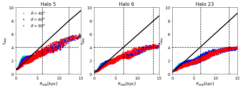
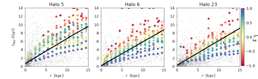
Figure 15: Upper panels: correlation of $t_{\rm dep}$ and elliptical radius $R_{\rm ellp}$ for all nine mock galaxies. $t_{\rm dep}$ at each position is derived by ($t_{\rm obs}$, $Z_{\rm obs}$) according to the theoretic relation $Z(t|t_{\rm dep})$ in Figure 4. The two vertical dashed lines in each panel indicate $R_{e}$ and $2R_{e}$. The thick black lines $t_{\rm dep}(r)=ar+b$ are determined by two points: (0, $t_{\rm dep,min}$) and ($R_{e}$, 4 Gyr). Bottom panels: correlation of $t_{\rm dep}$ and intrinsic radius $r$ in the three simulations. The gray dots represent particles in the simulation, the colored dots denote particles binned in the phase space $r$ vs. $\lambda_{z}$, colored by their circularity $\lambda_{z}$ as shown by the colorbar. The black lines are the same as the upper panels. Note that the y axis has different scales in the upper and bottom panels.

Appendix B Figures for all nine galaxies

Similar to figures we show for the galaxy Au-6 $\vartheta=80^{o}$ in Section 4. Figure 16 shows the stellar orbit distribution on $r$ vs. $\lambda_{z}$ comparing with the true from simulation and those from our models for all nine galaxies. Figure 17 and Figure 18 show the stellar population distribution $t$ vs. $Z$ from our models for all nine galaxies, with different priors of R1 and R2, respectively. Figure 19 and Figure 20 are the correlation of age $t$ and circularity $\lambda_{z}$ for all nine galaxies, with different priors of R1 and R2, respectively.

Similar to figures we show fro Au-6 $\vartheta=80^{o}$ in Section 5. Figure 21 are surface brightness, mean velocity, velocity dispersion, age and metallicity maps of cold, warm, hot+CR components, comparing with true from simulation with our model R2, for Au-5 $\vartheta=80^{o}$ and Au-23 $\vartheta=80^{o}$. Figure 22 are the age, metallicity profiles along major axis.

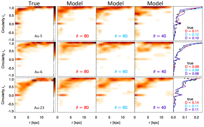
Figure 16: The stellar orbit distribution in $\lambda_{z}$ vs. $r$, for Au-5, Au-6, Au-23 from top to bottom. The first column is the true stellar orbit distributions from simulations. The rest columns are the distribution of orbits in our best-fitting models for mock data with $\vartheta=80^{o},60^{o},40^{o}$ from left to right. The last column is the marginalized $\lambda_{z}$ distribution. The black dashed curves are the true from simulations, red, blue, purple solid curves represent those from models for mock data with $\vartheta=80^{o},60^{o},40^{o}$, respectively. The D-statistics $D$ calculated from KS test comparing total $\lambda_{z}$ distribution from our model to the true from simulations are labeled with the corresponding colors.

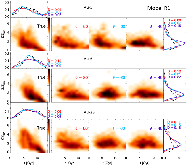
Figure 17: The intrinsic age-metallicity distribution, for Au-5, Au-6, Au-23 from top to bottom, for model R1. For each halo, the panel labeled with ‘True’ is the true distribution on Age vs. $Z$ of particles in the simulation. The following panels from left to right are those obtained by our model for mock data with inclination angle $\vartheta$ of $\vartheta=80^{o},60^{o},40^{o}$, respectively. The contours are smoothed by the distribution of $t$ and $Z$ from MCMC sampling. The upper subpanel is the marginalized age distribution and the right sub-panel is the marginalized metallicity $Z$ distribution. The black dashed curve is the true, red, blue, purple solid curves represent that from model for mock data with $\vartheta=80^{o},60^{o},40^{o}$, respectively, the D-statistics $D$ calculated from 1D KS test are labeled with the corresponding colors.

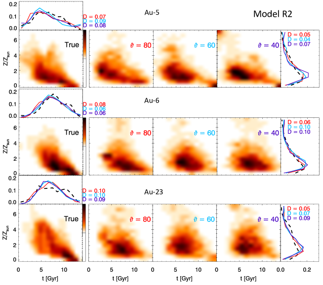
Figure 18: Similar to Figure 17, but with Model R2. The major tracks on age vs. metallicity distribution are recovered better than model R1, the D-statistics $D$ from 1D KS test for metallicity distribution are also smaller.

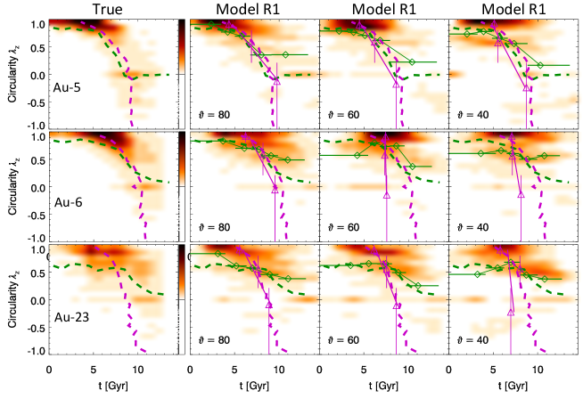
Figure 19: The intrinsic correlation of age vs circularity, for Au-5, Au-6, Au-23 from top to bottom, for model R1. The First column are true distributions of the particles from simulations, darker color indicates higher probability density, the magenta dashed curves are average $t$ as a function of $\lambda_{z}$, while the green dashed curves are average $\lambda_{z}$ as a function of age $t$ for the true distributions. The following panels from left to right are those obtained by our models for mock data with inclination angle $\vartheta$ of $\vartheta=80^{o},60^{o},40^{o}$, respectively. In each panel, the magenta triangles are average $t$ as a function of $\lambda_{z}$, the magenta lines are linear fits to the triangles. While the green diamonds are average $\lambda_{z}$ as a function of age $t$ from the model.

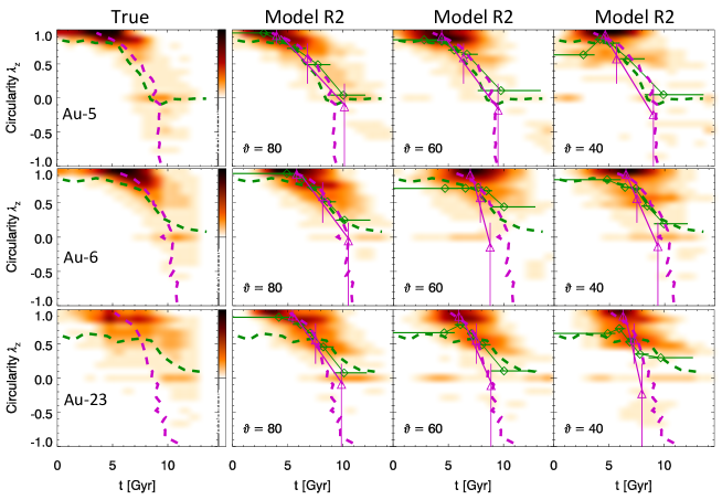
Figure 20: Similar to figure 19, but for model R2, in which we use $t=t_{0}+p\lambda_{z}$ (the blue line fitting the blue triangles) from model R1 as priors of $t_{k}$ in fitting the age map. Model R2 matches the age vs. $\lambda_{z}$ correlation in the simulation better than Model R1, especially for face-on galaxies.

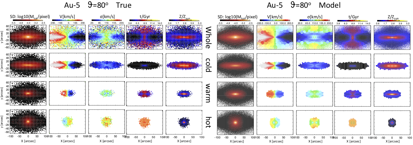
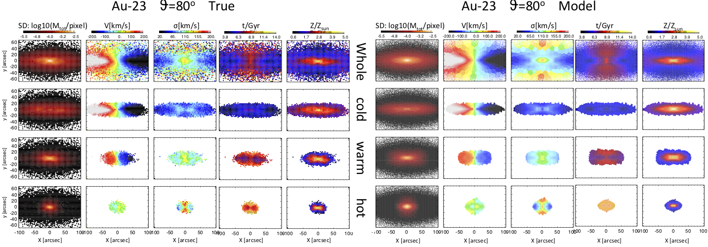
Figure 21: Surface mass density/brightness, mean velocity, velocity dispersion, age, and metallicity maps of the the whole galaxy, cold, warm, and hot + CR component (from top tp bottom) of Au-5 $\vartheta=80^{o}$ and Au-23 $\vartheta=80^{o}$. The left panels are the true values from the simulation, the right panels are rebuilt by orbital bundles from our model R2. These galaxies are at a distance of 30 Mpc, $1^{\prime\prime}=145\,{\rm pc}$.

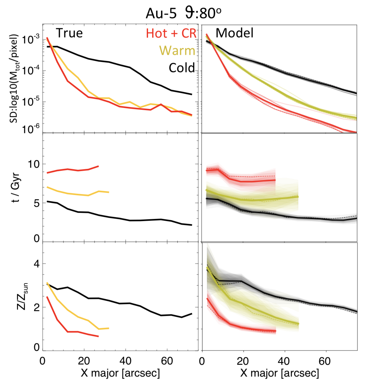
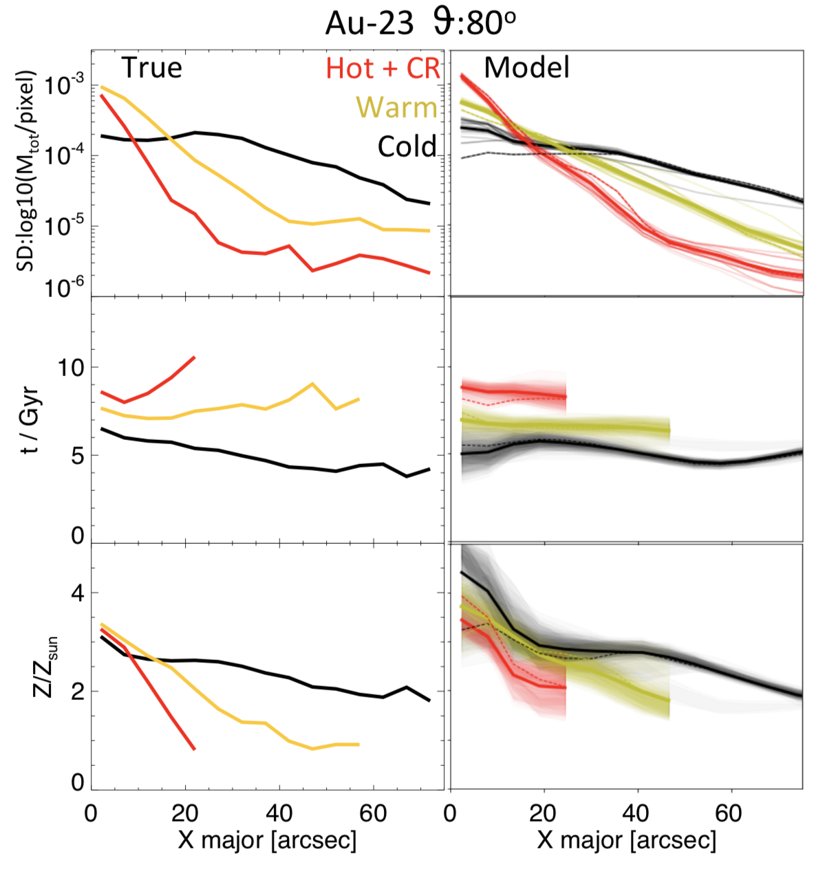
Figure 22: Surface mass density/brightness profile, age, and metallicity along major axis ($1^{\prime\prime}=145\,{\rm pc}$) of the cold, warm, and hot component, comparison between true and those built by model, similar to Figure 10 for Au-6 $\vartheta=80^{o}$. We generally recover the surface brightness, age and metallicity profiles of each component well. Except for Au-23, we over-estimate metallicity of cold component in the inner regions, thus resulting in a stronger negative metallicity gradient of this component than the true.

References

- Aumer, Binney & Schönrich (2016) Aumer M., Binney J., Schönrich R., 2016, MNRAS, 462, 1697
- Belokurov et al. (2018) Belokurov V., Erkal D., Evans N. W., Koposov S. E., Deason A. J., 2018, MNRAS, 478, 611
- Belokurov et al. (2019) Belokurov V., Sanders J. L., Fattahi A., Smith M. C., Deason A. J., Evans N. W., Grand R. J. J., 2019, arXiv e-prints, arXiv:1909.04679
- Benson et al. (2004) Benson A. J., Lacey C. G., Frenk C. S., Baugh C. M., Cole S., 2004, MNRAS, 351, 1215
- Bigiel et al. (2011) Bigiel F. et al., 2011, ApJL, 730, L13
- Bird et al. (2013) Bird J. C., Kazantzidis S., Weinberg D. H., Guedes J., Callegari S., Mayer L., Madau P., 2013, ApJ, 773, 43
- Boecker et al. (2019) Boecker A., Leaman R., van de Ven G., Norris M. A., Mackereth J. T., Crain R. A., 2019, MNRAS, 2678
- Bundy et al. (2015) Bundy K. et al., 2015, ApJ, 798, 7
- Cappellari (2002) Cappellari M., 2002, MNRAS, 333, 400
- Cappellari (2017) Cappellari M., 2017, MNRAS, 466, 798
- Carnall et al. (2019) Carnall A. C., Leja J., Johnson B. D., McLure R. J., Dunlop J. S., Conroy C., 2019, ApJ, 873, 44
- Cid Fernandes et al. (2005) Cid Fernandes R., Mateus A., Sodré L., Stasińska G., Gomes J. M., 2005, MNRAS, 358, 363
- Cretton & van den Bosch (1999) Cretton N., van den Bosch F. C., 1999, ApJ, 514, 704
- Croom et al. (2012) Croom S. M. et al., 2012, MNRAS, 421, 872
- de Lorenzi et al. (2007) de Lorenzi F., Debattista V. P., Gerhard O., Sambhus N., 2007, MNRAS, 376, 71
- Dutton & Macciò (2014) Dutton A. A., Macciò A. V., 2014, MNRAS, 441, 3359
- Emsellem, Monnet & Bacon (1994) Emsellem E., Monnet G., Bacon R., 1994, A&A, 285, 723
- Fattahi et al. (2019) Fattahi A. et al., 2019, MNRAS, 484, 4471
- Few et al. (2012) Few C. G., Gibson B. K., Courty S., Michel-Dansac L., Brook C. B., Stinson G. S., 2012, A&A, 547, A63
- Gaia Collaboration et al. (2018) Gaia Collaboration et al., 2018, A&A, 616, A1
- Gebhardt et al. (2000) Gebhardt K. et al., 2000, AJ, 119, 1157
- Genzel et al. (2011) Genzel R. et al., 2011, ApJ, 733, 101
- Gerhard (1993) Gerhard O. E., 1993, MNRAS, 265, 213
- Gómez et al. (2017) Gómez F. A. et al., 2017, MNRAS, 472, 3722
- Grand et al. (2017) Grand R. J. J. et al., 2017, MNRAS, 467, 179
- Grand et al. (2016) Grand R. J. J., Springel V., Gómez F. A., Marinacci F., Pakmor R., Campbell D. J. R., Jenkins A., 2016, MNRAS, 459, 199
- Grand et al. (2019) Grand R. J. J. et al., 2019, MNRAS, 490, 4786
- Guérou et al. (2016) Guérou A., Emsellem E., Krajnović D., McDermid R. M., Contini T., Weilbacher P. M., 2016, A&A, 591, A143
- Helmi et al. (2018) Helmi A., Babusiaux C., Koppelman H. H., Massari D., Veljanoski J., Brown A. G. A., 2018, Nature, 563, 85
- Helmi et al. (2012) Helmi A., Sales L. V., Starkenburg E., Starkenburg T. K., Vera-Ciro C. A., De Lucia G., Li Y. S., 2012, ApJL, 758, L5
- House et al. (2011) House E. L. et al., 2011, MNRAS, 415, 2652
- Hunt & Kawata (2014) Hunt J. A. S., Kawata D., 2014, MNRAS, 443, 2112
- Jenkins & Binney (1990) Jenkins A., Binney J., 1990, MNRAS, 245, 305
- Jin et al. (2019) Jin Y., Zhu L., Long R. J., Mao S., Xu D., Li H., van de Ven G., 2019, MNRAS, 486, 4753
- Kirby et al. (2013) Kirby E. N., Cohen J. G., Guhathakurta P., Cheng L., Bullock J. S., Gallazzi A., 2013, ApJ, 779, 102
- Leaman (2012) Leaman R., 2012, AJ, 144, 183
- Leaman et al. (2017) Leaman R. et al., 2017, MNRAS, 472, 1879
- Leaman, VandenBerg & Mendel (2013) Leaman R., VandenBerg D. A., Mendel J. T., 2013, MNRAS, 436, 122
- Leja et al. (2019) Leja J., Carnall A. C., Johnson B. D., Conroy C., Speagle J. S., 2019, ApJ, 876, 3
- Long (2016) Long R. J., 2016, Research in Astronomy and Astrophysics, 16, 189
- Long & Mao (2010) Long R. J., Mao S., 2010, MNRAS, 405, 301
- Long & Mao (2018) Long R. J., Mao S., 2018, Research in Astronomy and Astrophysics, 18, 145
- Mackereth et al. (2017) Mackereth J. T. et al., 2017, MNRAS, 471, 3057
- Marinacci et al. (2017) Marinacci F., Grand R. J. J., Pakmor R., Springel V., Gómez F. A., Frenk C. S., White S. D. M., 2017, MNRAS, 466, 3859
- McDermid et al. (2015) McDermid R. M. et al., 2015, MNRAS, 448, 3484
- Oey (2000) Oey M. S., 2000, ApJL, 542, L25
- Pakmor et al. (2017) Pakmor R. et al., 2017, MNRAS, 469, 3185
- Pinna et al. (2019a) Pinna F. et al., 2019a, arXiv e-prints
- Pinna et al. (2019b) Pinna F. et al., 2019b, A&A, 623, A19
- Pizzella et al. (2018) Pizzella A., Morelli L., Coccato L., Corsini E. M., Dalla Bontà E., Fabricius M., Saglia R. P., 2018, A&A, 616, A22
- Poci et al. (2019) Poci A., McDermid R. M., Zhu L., van de Ven G., 2019, MNRAS, 487, 3776
- Portail et al. (2017) Portail M., Wegg C., Gerhard O., Ness M., 2017, MNRAS, 470, 1233
- Rix et al. (1997) Rix H.-W., de Zeeuw P. T., Cretton N., van der Marel R. P., Carollo C. M., 1997, ApJ, 488, 702
- Ruiz-Lara et al. (2016) Ruiz-Lara T., Few C. G., Gibson B. K., Pérez I., Florido E., Minchev I., Sánchez-Blázquez P., 2016, A&A, 586, A112
- Sánchez et al. (2012) Sánchez S. F. et al., 2012, A&A, 538, A8
- Sarzi et al. (2018) Sarzi M. et al., 2018, A&A, 616, A121
- Springel (2010) Springel V., 2010, MNRAS, 401, 791
- Stinson et al. (2013) Stinson G. S. et al., 2013, MNRAS, 436, 625
- Tabor et al. (2019) Tabor M., Merrifield M., Aragón-Salamanca A., Fraser-McKelvie A., Peterken T., Smethurst R., Drory N., Lane R. R., 2019, MNRAS, 485, 1546
- Trayford et al. (2018) Trayford J. W., Frenk C. S., Theuns T., Schaye J., Correa C., 2018, ArXiv e-prints
- Tsatsi et al. (2015) Tsatsi A., Macciò A. V., van de Ven G., Moster B. P., 2015, ApJL, 802, L3
- Valluri, Merritt & Emsellem (2004) Valluri M., Merritt D., Emsellem E., 2004, ApJ, 602, 66
- van de Ven, de Zeeuw & van den Bosch (2008) van de Ven G., de Zeeuw P. T., van den Bosch R. C. E., 2008, MNRAS, 385, 614
- van den Bosch et al. (2008) van den Bosch R. C. E., van de Ven G., Verolme E. K., Cappellari M., de Zeeuw P. T., 2008, MNRAS, 385, 647
- van der Marel & Franx (1993) van der Marel R. P., Franx M., 1993, ApJ, 407, 525
- van der Wel et al. (2016) van der Wel A. et al., 2016, ApJS, 223, 29
- Vasiliev & Valluri (2019) Vasiliev E., Valluri M., 2019, arXiv e-prints, arXiv:1912.04288
- Wisnioski et al. (2015) Wisnioski E. et al., 2015, ApJ, 799, 209
- Zhu et al. (2018a) Zhu L. et al., 2018a, Nature Astronomy, 2, 233
- Zhu et al. (2018b) Zhu L. et al., 2018b, MNRAS, 473, 3000
Acknowledgments
This research is supported by the National Key RD Program of China under grant No. 2018YFA0404501 (SM, LZ), and National Natural Science Foundation of China under grant No. Y945271001 (LZ). GvdV and PJ acknowledges funding from the European Research Council (ERC) under the European Union’s Horizon 2020 research and innovation programme under grant agreement No 724857 (Consolidator Grant ArcheoDyn). J. F-B acknowledges support through the RAVET project by the grant AYA2016-77237-C3-1-P from the Spanish Ministry of Science, Innovation and Universities (MCIU) and through the IAC project TRACES which is partially supported through the state budget and the regional budget of the Consejería de Economía, Industria, Comercio y Conocimiento of the Canary Islands Autonomous Community. RMcD is the recipient of an Australian Research Council Future Fellowship (project number FT150100333).