Wave Turbulence in Self-Gravitating Bose Gases and Nonlocal Nonlinear Optics

Abstract

We develop the theory of weak wave turbulence in systems described by the Schrödinger-Helmholtz equations in two and three dimensions. This model contains as limits both the familiar cubic nonlinear Schrödinger equation, and the Schrödinger-Newton equations. The latter, in three dimensions, are a nonrelativistic model of fuzzy dark matter which has a nonlocal gravitational self-potential, and in two dimensions they describe nonlocal nonlinear optics in the paraxial approximation. We show that in the weakly nonlinear limit the Schrödinger-Helmholtz equations have a simultaneous inverse cascade of particles and a forward cascade of energy. We interpret the inverse cascade as a nonequilibrium condensation process, which is a precursor to structure formation at large scales (for example the formation of galactic dark matter haloes or optical solitons). We show that for the Schrödinger-Newton equations in two and three dimensions, and in the two-dimensional nonlinear Schrödinger equation, the particle and energy fluxes are carried by small deviations from thermodynamic distributions, rather than the Kolmogorov-Zakharov cascades that are familiar in wave turbulence. We develop a differential approximation model to characterise such “warm cascade” states.

I Introduction

I.1 Wave turbulence cascades

The dynamical and statistical behaviour of random weakly-interacting waves is responsible for many important physical effects across applications ranging from quantum to classical and to astrophysical scales (zakharov1992kolmogorovbook, ; nazarenko2011waveturbbook, ). Assuming weak nonlinearity and random phases, such behaviour is described by the theory of weak wave turbulence (zakharov1992kolmogorovbook, ; nazarenko2011waveturbbook, ). As in the theory of classical hydrodynamic turbulence, weak wave turbulence theory can predict nonequilibrium statistical states characterised by cascades of energy and/or other invariants through scales. Sometimes, similarly to 2D classical turbulence, such cascades are dual, with one invariant cascading to small scales (direct cascade) and the other invariant towards large scales (inverse cascade). An inverse cascade often leads to accumulation of the turbulence spectrum near the largest scale of the system, which is analogous to Bose-Einstein condensation. Large-scale coherent structures may form out of such a condensate and further evolve via mutual interactions and interactions with the background of random waves, thereby realising a scenario of order emerging from chaos.

In the present paper, we will study a precursor to such a process of coherent structure formation by developing the wave turbulence theory and describing the dual cascade in the so-called “Schrödinger-Helmholtz equations” that arise in cosmological and nonlinear optics applications.

I.2 Schrödinger-Helmholtz equations

The Schrödinger-Helmholtz equations are the nonlinear partial differential equations

$$i\partial_{t}\psi+\nabla^{2}\psi-V[\psi]\psi =0\,,$$ (1a)

$$\nabla^{2}V-\Lambda V =\gamma\lvert\psi\rvert^{2}$$ (1b)

for a complex scalar field $\psi(\mathbf{x},t)$ in which $V[\psi]$ plays the role of (potential) interaction energy and $\Lambda$ and $\gamma$ are constants. We will be interested in systems set in three and two spatial dimensions (3D and 2D, respectively).

Before proceeding in the body of the paper with developing the statistical description of the nonlinear field $\psi$ in the framework of Eqs. (1), we will first outline in this Sec. I.2 the important physical contexts in which Eqs. (1) have been used, the previous results found, and the findings that we anticipate will arise from our approach.

Notice that depending on the spatial scale of interest $\ell$, one term or the other on the left-hand side of Eq. (1b) is dominant. For $\ell\gg\ell_{*}=1/\sqrt{\Lambda}$ the Schrödinger-Helmholtz equations (1) become the more familiar cubic nonlinear Schrödinger equation, discussed in Sec. I.2.1, while for $\ell\ll\ell_{*}$ they turn into the Schrödinger-Newton equations, see Sec. I.2.2. Finally, in Sec. I.2.3 we return to interpret the Schrödinger-Helmholtz Eqs. (1) in light of the discussion of these limits.

I.2.1 Large-scale limit: The nonlinear Schrödinger equation

In the limit of large scales, $\ell\gg\ell_{*}$, the first term on the left-hand side of Eq. (1b) can be neglected and one immediately finds that $V[\psi]=-(\gamma/\Lambda)|\psi|^{2}$. The constant $\gamma/\Lambda$ can be removed by proper renormalization of $|\psi|^{2}$, leaving only the sign of this constant, denoted as $s=\pm 1$. Thus the Schrödinger-Helmholtz Eqs. (1) become the nonlinear Schrödinger equation

$$i\partial_{t}\psi+\nabla^{2}\psi+s\lvert\psi\rvert^{2}\psi=0\,,$$ (2)

also known as the Gross-Pitaevskii equation (pitaevskiistringari2016book, ). This equation has a cubic, spatially local, attractive (for $s=+1$) or repulsive (for $s=-1$) interaction.

The nonlinear Schrödinger  Eq. (2) is well known in the study of Bose-Einstein condensates (pitaevskiistringari2016book, ), where $\psi$ is the wavefunction of a system of identical bosons in the Hartree-Fock approximation (gross_structure_1961, ; pitaevskii_vortex_1961, ) and the nonlinearity is due to $s$-wave scattering. (As well as normalising the coupling constant $s$ to $\pm 1$, units are further chosen such that the reduced Planck constant $\hbar=1$ and the boson mass $m=1/2$.)

Equation (2) is also familiar in the field of nonlinear optics (newellmoloney1992nonlinearopticsbook, ; boyd2008nonlinearopticsbook, ) when a light beam, whose electric field is slowly modulated by an envelope $\psi$ (such that its intensity is $\lvert\psi\rvert^{2}$), impinges on a dispersive, nonlinear medium, inducing a nonlinear change in the medium’s refractive index via the Kerr effect. Equation (2) then describes the evolution of the beam’s envelope in the paraxial approximation, where $t$ becomes the length along the beam axis, and the remaining spatial directions are transverse to the beam. (In the optics application units are chosen such that $k_{0}n_{0}=1/2$ where $k_{0}$ is the free space wavenumber of the input beam and $n_{0}$ is the refractive index of the medium, normalising the coefficient of the Laplacian term to unity.)

In this context $s$ is the normalised Kerr coefficient, and the cases with $s=+1$ or $-1$ are known as the focusing or defocusing nonlinear Schrödinger equation respectively, terminology that we adopt here in the general case.

The nonlinear Schrödinger Eq. (2) is studied in a great many other systems due to its universality in describing the slowly-varying envelope of a monochromatic wave in a weakly nonlinear medium (whitham1999waves, ). We shall not pursue its other applications in this work, instead merely noting that due to its universality many monographs and papers have been dedicated to the study of Eq. (2) and its solutions.

I.2.2 Small-scale limit: The Schrödinger-Newton equations

Now we focus on scales $\ell\ll\ell_{*}$, when the second term in the left-hand side of Eq. (1b) dominates. Then the Schrödinger-Helmholtz Eqs. (1) simplify to the coupled equations

$$i\partial_{t}\psi+\nabla^{2}\psi-V[\psi]\psi =0\,,$$ (3a)

$$\nabla^{2}V =\gamma\lvert\psi\rvert^{2}\,.$$ (3b)

In three dimensions if we retain the interpretation of $\psi(\mathbf{x},t)$ as a boson wavefunction, we see that the nonlinearity in Eq. (3a) is nonlocal, coming from an extended potential $V[\psi]$ that solves the Poisson Eq. (3b) for which the source is proportional to the boson number density $\rho=\lvert\psi\rvert^{2}$. Specifying $\gamma=\pi$, and noting that we have chosen units in which $\hbar=1$, $m=1/2$, and Newton’s gravitational constant $G=1$, we observe that Eqs. (3) describe a dilute Bose gas moving at nonrelativistic speeds under the influence of a Newtonian gravitational potential generated by the bosons themselves. It is for this reason that Eqs. (3) are known as the Schrödinger-Newton equations. (The derivation of Eqs. (3) from a Klein-Gordon action with a general relativistic metric can be found in the literature, for example (marsh2016axion, ; niemeyer2020small, ).)

The use of Eqs. (3) to represent self-gravitating Bose gases in the Newtonian limit is important in cosmology, where they are used to model “fuzzy dark matter”. This is the hypothesis that dark matter is comprised of ultra-light ($m\lesssim$1\text{\times}{10}^{-22}\text{\,}\mathrm{eV}$$) scalar bosons whose de Broglie wavelengths are on the order of galaxies ($\lambda_{\mathrm{dB}}\sim$1\text{\,}\mathrm{kpc}$$) (HuFuzzy2000, ; SuarezBECDM2014, ; Chavanis2015_SelfGravBECs, ; marsh2016axion, ; hui2017ultralight, ; ferreira2020ultra, ). In this scenario galactic dark matter haloes are gigantic condensates of this fundamental boson, trapped by their own gravity and supported by quantum pressure arising from the uncertainty principle (HuFuzzy2000, ; baldeschi1983massive, ; lee1996galactic, ; Chavanis2015_SelfGravBECs, ; schive2014cosmic, ; verma2019formation, ; niemeyer2020small, ).

Fuzzy dark matter is an alternative to the standard model of cosmology which supposes that dark matter is comprised of thermal but sub-luminal, weakly interacting massive particles, i.e., “cold dark matter” (OverduinWesson_WIMPs_2004, ). While cold dark matter is successful at describing the observed large-scale structure of the universe, its accelerated expansion, and the fluctuations of the cosmic microwave background (PeeblesRatra_CDM_2003, ; Springel_CDM_2005, ), at small scales it fails to reconcile observations with cosmological simulations, particularly in matching the inferred flat density profiles of galactic dark matter haloes with the cuspy profiles found in simulations, and the lack of observed satellite dwarf galaxies as compared to theoretical predictions (Weinberg_SmallScaleControv_2015, ; Bullock_SmallScaleControv_2017, ). By contrast, in fuzzy dark matter galactic cores arise naturally as compact soliton-like objects structures with core radii on the order of $\lambda_{\mathrm{dB}}$, below which fine structure is suppressed by the uncertainty principle (harko2011bose, ; marsh2015axion, ) and, when included in the model, $s$-wave scattering (Chavanis2015_SelfGravBECs, ; lee1996galactic, ; colpi1986boson, ), providing a resolution to the small-scale problems of cold dark matter. At large scales the two models become indistinguishable (schive2014cosmic, ). Thus, until the precise nature of dark matter particles is identified, fuzzy dark matter must be considered alongside cold dark matter when investigating the formation of large-scale structure in the early universe (schive2014cosmic, ; mocz2017galaxyI, ; mocz2019first, ; mocz2019galaxyII, ).

Like the nonlinear Schrödinger  Eq. (2), the Schrödinger-Newton Eqs. (3) also have applications in nonlinear optics. Here (3a) is again the equation for the envelope of the beam in two transverse spatial dimensions and the distance along the beam is again the time-like dimension. $V[\psi]$ is now the change in refractive index of the optical sample induced by the incident beam, whose nonlocality is expressed in Eq. (3b). This can be due to the refractive index being temperature-dependent and (3b) describing the diffusion of the incident beam energy through the medium as heat: the thermo-optic effect (boyd2008nonlinearopticsbook, ; castillo1996formation, ). Alternatively, in nematic liquid crystals the refractive index depends on the orientation of the liquid crystal molecules with respect to the wavevector of the incident beam, and (3b) describes the reorientation induced by the electric (or magnetic) field of the beam, which diffuses through the sample due to long-range elastic interactions between the molecules (khoo2007liquidcrystalsbook, ).

Nonlocal nonlinear optics manifest many phenomena that are the nonlocal versions of the equivalent local phenomenon, for example (but by no means limited to) solitons (snyder1997accessible, ; castillo1996formation, ; conti2003route, ; rotschild2005ellipticsolitons, ), soliton interactions (rotschild2006long, ), modulational instability and collapse (perez2000dynamics, ; bang2002collapse, ; peccianti2003optical, ), and shocks and shock turbulence (ghofraniha2007shocks, ; xu2015coherent, ). In addition, comparisons can be made between nonlinear optical systems and fuzzy dark matter by virtue of Eqs. (3) describing them both. Indeed recent optics experiments (Faccio2016_OpticalNewtSchro, ; Beckenstein2015_OpticalNewtSchro, ), and theoretical works (navarrete2017spatial, ; paredes2020optics, ) have drawn direct analogies between optical systems that can be realised in the laboratory and astrophysical systems on the scale of galaxies.

I.2.3 Physical applications of the Schrödinger-Helmholtz equations

The Schrödinger-Helmholtz Eqs. (1), then, are a model that captures the physics present in both Eq. (2) and Eqs. (3). Applied to fuzzy dark matter the diffusive term in Eq. (1b) represents gravity in the Newtonian approximation of the Einstein field equations, as per Sec. I.2.2, while the local term corresponds to the inclusion of a cosmological constant $\Lambda$ in this approximation (kiessling2003jeans, ). This is necessary if one wants to account for a dark energy component to cosmology in a Newtonian approximation. It is also a means to regularise the so-called “Jeans swindle”—the specification that Eq. (3b) only relates the fluctuations of density and potential around an unspecified equilibrium (BinneyTremaine1987_GalacDynBook, ), see Appendix A.

In the optical context Eqs. (1) model a system where both Kerr (local) effects and thermo-optic or elastic (diffusive nonlocal) effects are important (alternatively, the diffusive term in Eq. (1b) can be used to take account of heat losses at the edges of the optical sample (ghofraniha2007shocks, ; Faccio2016_OpticalNewtSchro, )).

We therefore take the Schrödinger-Helmholtz Eqs. (1), as our model of interest as they comprise a model that is physically relevant in both astrophysics and nonlinear optics, depending on the choice of dimensionality and units. They contain as limits both the nonlinear Schrödinger equation, about which much is known, and the Schrödinger-Newton equations, whose relevance is starting to come to the fore. Next we discuss weak and strong turbulence in these latter models, and introduce the process of dual cascade of invariants, which is a precursor to the formation of structures at the largest scale in Schrödinger-Helmholtz systems.

I.3 Turbulence in the nonlinear Schrödinger and Schrödinger-Newton equations

Turbulence in laboratory Bose-Einstein condensates (Vinen2002QTurb, ; barenghi2001quantized, ; kobayashi2007quantum, ; krstulovic2011dispersive, ; tsatsos_quantum_2016, ; tsubota2017numerical, ; muller2020abrupt, ) and optics (LaurieEtAl2012_1DOpticalWT, ; dyachenko1992optical, ; picozzi2014optical, ) is now a well-established field, and much has been understood by using the local nonlinear Schrödinger Eq. (2). Its dynamics is rich, with weakly nonlinear waves typically coexisting with coherent, strongly nonlinear structures. The nature of these structures depends radically on the sign of the interaction term $s$ in Eq. (2). In the defocusing (repulsive) case they include stable condensates: accumulations of particles (in the Bose-Einstein condensate case) or intensity (optics) at the largest scale, with turbulence manifesting as a collection of vortices in 2D, or a tangle of vortex lines in 3D, on which the density is zero and which carry all the circulation, propagating through the condensate (tsatsos_quantum_2016, ; tsubota2017numerical, ; nazarenko2011waveturbbook, ). In the focusing (attractive) case solitons and condensates are unstable above a certain density, with localised regions of over-density collapsing and becoming singular in finite time (dyachenko1992optical, ; sulem1999nonlinear, ).

On the other hand, turbulence in the Schrödinger-Newton Eqs. (3) has only recently been investigated by direct numerical simulation in the cosmological setting (mocz2017galaxyI, ) and appears to contain features of both the focusing and the defocusing nonlinear Schrödinger equation. As mentioned above, at large scales the Schrödinger-Newton model exhibits gravitationally-driven accretion into filaments which then become unstable and collapse into spherical haloes (mocz2019first, ; mocz2019galaxyII, ) (cf. collapses in the focusing nonlinear Schrödinger model driven by the self-focusing local contact potential). However, within haloes the condensate is stable, with turbulence in an envelope surrounding the core manifesting as a dynamic tangle of reconnecting vortex lines, as in the defocusing nonlinear Schrödinger model (mocz2017galaxyI, ). This is to be expected, given that the attractive feature of the Schrödinger-Newton model in cosmology is that it is simultaneously unstable to gravitational collapse and stable once those collapse event have regularised into long-lived structures, and so it should contain features of both the unstable (focusing) and stable (defocusing) versions of the nonlinear Schrödinger model.

To understand more fully the phenomenology recently reported in the Schrödinger-Newton Eqs. (3), it is tempting to apply theoretical frameworks that have been successful in explaining various aspects of turbulence in the nonlinear Schrödinger equation. One such theory is wave turbulence: the study of random broadband statistical ensembles of weakly interacting waves (nazarenko2011waveturbbook, ; zakharov1992kolmogorovbook, ). The “turbulent” behaviour referred to here is the statistically steady-state condition where dynamically conserved quantities cascade through scales in the system via the interaction of waves, a process analogous to the transfer of energy in 3D classical fluid turbulence (and respectively energy and enstrophy in 2D). Wave turbulence theory is integral to the quantitative description of both the wave component and the evolution of the coherent components of the nonlinear Schrödinger system and is relevant in three regimes: de Broglie waves propagating in the absence of a condensate (dyachenko1992optical, ; nazarenko2011waveturbbook, ), Bogoliubov acoustic waves on the background of a strong condensate (dyachenko1992optical, ; nazarenko2011waveturbbook, ), and Kelvin waves that are excited on quantized vortex lines in a condensate (nazarenko2011waveturbbook, ; lvovnazarenko2010kelvin, ). If the system is focusing, then the condensate is modulationally unstable and vortices do no appear, so acoustic and Kelvin wave turbulence will not be realised [the gravitational-type nonlinearity present in Eqs. (3) is of focusing type and so this is the situation that is most relevant to this work]. Nonetheless, in both focusing and defocusing systems de Broglie wave turbulence theory describes how, starting from a random ensemble of waves, a dual cascade simultaneously builds up the large-scale condensate while sending energy to small scales (nazarenko2011waveturbbook, ). As we will describe in Sec. II.3 below, this dual cascade is generic in any system of interacting waves with two quadratic dynamical invariants (particles and energy in the cases of interest here). The theory of wave turbulence thus provides a universal description of how large-scale coherent structures can arise from a random background.

The wave turbulence of Eqs. (1), the fundamental process of dual cascade, and the spectra on which such cascades can occur, have already been investigated theoretically and in optics experiments in the one-dimensional case (BortolozzoEtAl2009_OpticalWTCondensnLight, ; LaurieEtAl2012_1DOpticalWT, ) in the large-scale and small-scale limits where the dynamical equations become Eq. (2) and Eqs. (3) respectively. To our knowledge such a study of the wave turbulence of (1) has not been made in higher dimensions. We begin this study in the current work.

Having said this, we note that Ref. (picozzi2014optical, ) refers to the “optical wave turbulence” of nonlocal systems, of which the Schrödinger-Helmholtz equations are an important example. Much of Ref. (picozzi2014optical, ), and references therein, pertains to the dynamics of inhomogeneous systems (such as modulational instability and collapse, studied by a Vlasov equation). By contrast here we are concerned with the dynamics that govern statistically homogeneous systems. We comment on the difference in approaches to inhomogeneous vs. homogeneous systems in Appendix B. Furthermore, a recent paper (levkov2018gravitational, ) has examined the formation of large-scale structure in astrophysical Bose gases obeying Eqs. (3), using a kinetic formulation which was termed“wave turbulence” in Ref. (niemeyer2020small, ). We describe the similarities and differences between Ref. (levkov2018gravitational, ) and this work in Sec. IV.1.

I.4 Organisation of this paper

In this work, then, we develop the theory of wave turbulence for the Schrödinger-Helmholtz Eqs. (1) in the case of fluctuations about a zero background. By taking the limits of small and large $\Lambda$ we obtain the wave turbulence of the Schrödinger-Newton Eqs. (3) and also review known results of the nonlinear Schrödinger Eq. (2). Our aim is to describe the fundamental dynamical processes that govern the first stages of formation of a large-scale condensate from random waves in cosmology and in nonlinear optics. From this structure gravitational-type collapses will ensue and the phenomenology described above will develop.

In Secs. II.1 and II.2 we overview the wave turbulence theory and arrive at the wave kinetic equation that describes the evolution of the wave content of the system. Section II.3 describes the dual cascade of energy towards small scales and particles towards large scales in the system. In Secs. II.4 and II.5 we describe respectively the scale-free pure-flux spectra and equilibrium spectra that are formal stationary solutions of the wave kinetic equation. However in Sec. II.6 we show that these stationary spectra yield the wrong directions for the fluxes of energy and particles, as compared with the directions predicted in Sec. II.3. We resolve this paradox by developing a reduced model of the wave dynamics in Secs. II.7 and II.8 and using it in Sec. III to reveal the nature of the dual cascades in the nonlinear Schrödinger and the Schrödinger-Newton limits of the Schrödinger-Helmholtz equations. We conclude in Sec. IV and suggest further directions of research incorporating wave turbulence into the study of the Schrödinger-Helmholtz equations.

II Building blocks of Schrödinger-Helmholtz wave turbulence

In this section we overview the aspects of the wave turbulence theory that we require in our description of turbulence in the Schrödinger-Helmholtz model.

II.1 Hamiltonian formulation of the Schrödinger-Helmholtz equations

To put Schrödinger-Helmholtz turbulence in the context of the general theory of wave turbulence we need to formulate the Schrödinger-Helmholtz Eqs. (1) in Hamiltonian form. For that goal we first set the system in the periodic box $\Omega=\mathbb{T}^{d}_{L}$ and decompose variables into Fourier modes

$$\psi_{\mathbf{k}}(t)=\frac{1}{L^{d}}\int_{\Omega}\!\psi(\mathbf{x},t)e^{-i\mathbf{k}\cdot\mathbf{x}}\,d\mathbf{x}\,,$$

and similarly for $V_{\mathbf{k}}(t)$. The dynamical equations become

$$i\partial_{t}\psi_{\mathbf{k}}-k^{2}\psi_{\mathbf{k}}-\sum_{1,2}V_{1}\psi_{2}\delta^{\mathbf{k}}_{12}=0\,,$$ (4a)

$$-(k_{1}^{2}+\Lambda)V_{1}=\gamma\sum_{3,4}\psi_{3}\psi_{4}^{*}\delta^{3}_{14}\,,$$ (4b)

where $V_{j}=V_{\mathbf{k}_{j}}$, $\psi_{j}=\psi_{\mathbf{k}_{j}}$, $\sum_{i\ldots j}=\sum_{\mathbf{k}_{i},\ldots,\mathbf{k}_{j}}$ and $\delta^{\mathbf{k}}_{12}=\delta(\mathbf{k}-\mathbf{k}_{1}-\mathbf{k}_{2})$ is the Kronecker delta, equal to unity if $\mathbf{k}=\mathbf{k}_{1}+\mathbf{k}_{2}$ and zero otherwise.

Equations (4) can be rewritten as the canonical Hamiltonian equation

$$i\partial_{t}\psi_{\mathbf{k}}={} \frac{\partial H}{\partial\psi_{\mathbf{k}}^{*}}\,,\qquad H=H_{2}+H_{4}\,,$$ (5a)

$$H_{2}={} \sum_{\mathbf{k}}\omega_{\mathbf{k}}\psi_{\mathbf{k}}\psi_{\mathbf{k}}^{*}\,,$$ (5b)

$$H_{4}={} -\frac{1}{2}\sum_{1234}W^{12}_{\,34}\psi_{1}\psi_{2}\psi_{3}^{*}\psi_{4}^{*}\delta^{12}_{34}\ .$$ (5c)

Here the Hamiltonian $$H H_{2} \omega_{\mathbf{k}}=k^{2} H_{4} 2\leftrightarrow 2 W^{12}_{\,34}$$ is comprised of the quadratic part , which leads to linear waves with dispersion relation , and the interaction Hamiltonian which describes four-wave coupling of the type. The interaction coefficient can written in the symmetric form

$$W^{12}_{\,34}={} \frac{\gamma}{4}\left(A_{1234}+A_{2134}+A_{1243}+A_{2143}\right)\,,$$ (5d)

$$A_{1234}={} 1\Big{/}\big{[}(\mathbf{k}_{1}-\mathbf{k}_{4})\cdot(\mathbf{k}_{3}-\mathbf{k}_{2})+\Lambda)\big{]}\ .$$ (5e)

If we are using the Jeans swindle from the outset (see Footnote 1) then the sum in Eq. (5c) must exclude all terms when any two wavenumbers are equal.

For completeness, we note that if we include a local cubic self-interaction term $-s\lvert\psi\rvert^{2}\psi$ on the right-hand side of Eq. (3a) as well as the gravitational term then the four-wave interaction coefficient would be

$$W^{12}_{\,34}=-s+\frac{\gamma}{4}\left(A_{1234}+A_{2134}+A_{1243}+A_{2143}\right),$$ (5f)

with $A_{1234}$ as in Eq. (5e). Finally, the four-wave interaction coefficient for the cubic nonlinear Schrödinger Eq. (2) is simply

$$W^{12}_{\,34}=-s\ .$$

II.2 Kinetic equation and conserved quantities

In the theory of weak wave turbulence we consider ensembles of weakly interacting waves with random phases uniformly distributed in $[0,2\pi)$, and independently distributed amplitudes (nazarenko2011waveturbbook, ; choi2004probability, ; choi2005joint, ; choi2009wave, ). We define the wave spectrum

$$n_{\mathbf{k}}=\left(\frac{L}{2\pi}\right)^{d}\langle\lvert\psi_{\mathbf{k}}\rvert^{2}\rangle\,,$$ (6)

where the angle brackets $\langle\ldots\rangle$ denote averaging of “$\ldots$” over the random phases and amplitudes.

In the limit of an infinite domain $L\to\infty$ and for weak nonlinearity $\lvert H_{4}/H_{2}\rvert\ll 1$ one can derive (dyachenko1992optical, ; nazarenko2011waveturbbook, ; zakharov1992kolmogorovbook, ) a wave kinetic equation for the evolution of the spectrum. For $2\leftrightarrow 2$ wave processes with the interaction Hamiltonian (5c), the kinetic equation is

$$\begin{split}\partial_{t}n_{\mathbf{k}}={}&4\pi\!\int\!\lvert W^{12}_{\,3\mathbf{k}}\rvert^{2}\delta^{12}_{3\mathbf{k}}\delta(\omega^{12}_{3\mathbf{k}})n_{1}n_{2}n_{3}n_{\mathbf{k}}\\ &\times\left[\frac{1}{n_{\mathbf{k}}}+\frac{1}{n_{3}}-\frac{1}{n_{1}}-\frac{1}{n_{2}}\right]\mathrm{d}\mathbf{k}_{1}\mathrm{d}\mathbf{k}_{2}\mathrm{d}\mathbf{k}_{3}\,,\end{split}$$ (7)

where $\delta^{12}_{3\mathbf{k}}$ is now a Dirac delta function that imposes wavenumber resonance $\mathbf{k}+\mathbf{k}_{3}=\mathbf{k}_{1}+\mathbf{k}_{2}$; likewise frequency resonance $\omega_{\mathbf{k}}+\omega_{3}=\omega_{1}+\omega_{2}$ is enforced by the Dirac delta $\delta(\omega^{12}_{3\mathbf{k}})$.

The kinetic equation (7) describes the irreversible evolution of an initial wave spectrum via four-wave interaction. It is the central tool of wave turbulence theory at the lowest level of closure of the hierarchy of moment equations (the theory also allows the study of higher moments or even the full probability density function (nazarenko2011waveturbbook, ; choi2004probability, ; choi2005joint, ; choi2009wave, )). Equation (7) allows one to study the dynamical evolution of a wave spectrum from an arbitrary initial condition, provided the interaction is weak. The spectra that are of greatest interest in wave turbulence theory are the stationary solutions that we discuss in Secs. II.4 and II.5. As well as being the first checkpoint in analysing the wave turbulence of a new system, these spectra also frequently characterise the time-dependent dynamics. We shall return to this point in Sec. IV.1.

As the spectrum evolves under the action of Eq. (7) the following two quantities are conserved by the kinetic equation

$$N={} \int\!n_{\mathbf{k}}\,\mathrm{d}\mathbf{k}\,,$$ (8a)

$$E={} \int\!\omega_{\mathbf{k}}n_{\mathbf{k}}\,\mathrm{d}\mathbf{k}\ .$$ (8b)

Here $N$ is known as the (density of) waveaction, or particle number, and is conserved for all times by the original Eqs. (1), and $E$ is referred to as the (density of) energy. It is the leading-order part of the total Hamiltonian, i.e., $H_{2}$, and is only conserved by Eqs. (1) over timescales for which the kinetic equation (7) is valid.

For isotropic systems such as Eqs. (1) we can express the conservation of invariants (8) as scalar continuity equations for the waveaction

$$\partial_{t}N_{k}^{\mathrm{(1D)}}+\partial_{k}\eta=0\,,\qquad N_{k}^{\mathrm{(1D)}}=\mathbb{A}^{(d-1)}n_{\mathbf{k}}k^{d-1}\,,$$ (9a)

and for the energy

$$\partial_{t}E_{k}^{\mathrm{(1D)}}+\partial_{k}\epsilon=0\,,\qquad E_{k}^{\mathrm{(1D)}}=\omega_{\mathbf{k}}N_{k}^{\mathrm{(1D)}}\ .$$ (9b)

Here $\eta=\eta(k)$ and $\epsilon=\epsilon(k)$ are, respectively, the flux of waveaction and energy through the shell in Fourier space of radius $k=\lvert\mathbf{k}\rvert$. In Eq. (9a) we have defined the isotropic 1-dimensional (1D) waveaction spectrum $N_{k}^{\mathrm{(1D)}}$, where $\mathbb{A}^{(d-1)}$ is the area of a unit $(d-1)$-sphere; likewise in Eq. (9b) $E_{k}^{\mathrm{(1D)}}$ is the isotropic 1D energy spectrum.

In the rest of this work we will consider a forced-dissipated system, with forcing in a narrow band at some scale $k_{\mathrm{f}}$ and dissipation at the large and small scales $k_{\mathrm{min}}$ and $k_{\mathrm{max}}$ respectively, and assume that these scales are widely separated $k_{\mathrm{min}}\ll k_{\mathrm{f}}\ll k_{\mathrm{max}}$. The interval $k_{\mathrm{f}}<k<k_{\mathrm{max}}$ is known as the direct inertial range, and $k_{\mathrm{min}}<k<k_{\mathrm{f}}$ is called the inverse inertial range, because of the directions that $E$ and $N$ flow through these ranges, as we describe in the next section. In this open setup the local conservation Eqs. (9) will hold deep inside the inertial ranges but the global quantities $N$ and $E$ are only conserved if the rates at which they are injected match their dissipation rates.

We examine the open system because it allows the nonequilibrium stationary solutions of Eq. (7) to form and persist, revealing the dual cascade in its purest manifestation. The alternative would be to study turbulence that evolves freely from an initial condition. In that case features of the stationary solutions still often characterise the evolving spectra, see Sec. IV.1. We leave the study of the time-evolving case to future work and here establish the forms of the stationary spectra by considering the forced-dissipative setup.

II.3 Fjørtoft argument for two conserved invariants

The presence of two dynamical invariants $E$ and $N$ whose densities differ by a monotonic factor of $k$, here by $\omega_{\mathbf{k}}=k^{2}$, places strong constraints on the directions in which the invariants flow through $\mathbf{k}$-space, as pointed out by Fjørtoft (fjortoft1953changes, ). We recapitulate his argument in its open-system form.

Consider the system in a steady state where forcing balances dissipation: at $k_{\mathrm{f}}$ energy and particles are injected at rate $\epsilon$ and $\eta$ respectively, and dissipated at those rates at $k_{\mathrm{min}}$ or $k_{\mathrm{max}}$. The ratio of the density of energy to the density of particles is $k^{2}$, and so the energy and particle flux must be related by the same factor at all scales. At the forcing scale this means that $\epsilon\sim k_{\mathrm{f}}^{2}\eta$.

The argument proceeds by contradiction. Suppose that the energy is dissipated at the large scale $k_{\mathrm{min}}$ at the rate $\sim\epsilon$ that it is injected. Then at this scale particles would be removed at rate $\sim\epsilon/k_{\mathrm{min}}^{2}\sim\eta k_{\mathrm{f}}^{2}/k_{\mathrm{min}}^{2}\gg\eta$ which is impossible because then the particle dissipation rate would exceed the rate of injection. Therefore in a steady state most of the energy must be dissipated at small scales $k_{\mathrm{max}}$. Likewise, if we assume the particles are removed at the small scale $k_{\mathrm{max}}$ at rate $\sim\eta$ then energy would be removed at the impossible rate $\sim\epsilon k_{\mathrm{max}}^{2}/k_{\mathrm{f}}^{2}\gg\epsilon$ so most of the particles must be removed at large scales $k_{\mathrm{min}}$ instead.

Therefore, this argument predicts that the scale containing most of the energy must move towards high $k$ while the scale containing the most particles must move towards low $k$. Particles are then removed if $k_{\mathrm{min}}$ represents a dissipation scale. However if there is no dissipation here then the spectrum develops a localised bump as the particles accumulate at the largest scale—this is the condensate. In this case $k_{\mathrm{min}}$ represents the transition scale between the condensate, which becomes strongly nonlinear as the dual cascade proceeds, and the weakly nonlinear wave component of the system which continues to obey Eq. (7).

It is thus the Fjørtoft argument that robustly predicts that particles accumulate at the largest available scale in the system, while energy is lost by the dissipation at $k_{\mathrm{max}}$, a process of simultaneous nonequilibrium condensation and “evaporative cooling” (lvov2003wave, ).

The Fjørtoft argument does not specify whether the invariants move via local scale-by-scale interactions, or by a direct transfer from the intermediate to the extremal scales. In the next Sec. II.4 we consider spectra on which the two invariants move via a local cascade.

II.4 Kolmogorov-Zakharov flux spectra as formal solutions of the kinetic equation

The landmark result of the theory of weak wave turbulence is the discovery of spectra on which invariants move with constant flux through $\mathbf{k}$-space via a local scale-by-scale cascade, potentially realising the predictions of the Fjørtoft argument. [However, anticipating the results of Sec. II.6, it turns out that for the Schrödinger-Newton Eqs. (3) and nonlinear Schrödinger Eq. (2) these spectra lead in most cases to cascades with the fluxes in the wrong direction, a contradiction that we resolve in the remainder of this work.] These are the Kolmogorov-Zakharov spectra (zakharov1992kolmogorovbook, ) and are analogous to Kolmogorov’s famous $k^{-5/3}$ energy cascade spectrum for 3D classical strongly-nonlinear hydrodynamical turbulence (Kolmogorov1941, ). When they exist, they are steady nonequilibrium solutions of the kinetic equation in which the spectra are scale-invariant, i.e.,

$$n_{\mathbf{k}}\propto k^{-x}.$$ (10)

Necessary (but not sufficient) conditions for such spectra to exist are that both the dispersion relation and interaction coefficient are themselves both scale-invariant. In our case the dispersion relation is $\omega_{\mathbf{k}}=k^{2}$. For the interaction coefficient we require a homogeneous function in the sense that

$$W^{\mu\mathbf{k}_{1}\,\mu\mathbf{k}_{2}}_{\,\mu\mathbf{k}_{3}\,\mu\mathbf{k}_{4}}=\mu^{\beta}W^{\mathbf{k}_{1}\,\mathbf{k}_{2}}_{\,\mathbf{k}_{3}\,\mathbf{k}_{4}}\ .$$

For the Schrödinger-Helmholtz Eqs. (1) we obtain a scale-invariant interaction coefficient in either the Schrödinger-Newton limit $\ell\ll\ell_{*}$ (in which case $\beta=-2$) or in the nonlinear Schrödinger limit $\ell\gg\ell_{*}$ (where $\beta=0$).

The Kolmogorov-Zakharov spectra are obtained by making a so-called Zakharov-Kraichnan transform in the kinetic equation (7) and using the scaling behaviour of all quantities under the integral (dyachenko1992optical, ; nazarenko2011waveturbbook, ; zakharov1992kolmogorovbook, ), or via dimensional analysis (nazarenko2011waveturbbook, ; connaughton2003dimensional, ). We omit the details and quote the results here.

For systems of $2\leftrightarrow 2$ wave scattering in $d$ spatial dimensions, the spectrum that corresponds to a constant flux of particles and zero flux of energy has index

$$x_{\scriptscriptstyle\mathrm{FN}}=d+\frac{2\beta}{3}-\frac{2}{3}\ .$$ (11a)

The spectrum of constant energy flux with zero particle flux is

$$x_{\scriptscriptstyle\mathrm{FE}}=d+\frac{2\beta}{3}\ .$$ (11b)

In particular for the Schrödinger-Newton Eqs. (3) we have $\beta=-2$, so

$$x_{\scriptscriptstyle\mathrm{FN}}=1\,, x_{\scriptscriptstyle\mathrm{FE}}=5/3 \mathrm{for} d=3\,,$$ (12a)

$$x_{\scriptscriptstyle\mathrm{FN}}=0\,, x_{\scriptscriptstyle\mathrm{FE}}=2/3 \mathrm{for} d=2\,,$$ (12b)

while for the nonlinear Schrödinger Eq. (2) $$\beta=0$$, so

$$x_{\scriptscriptstyle\mathrm{FN}}=7/3\,, x_{\scriptscriptstyle\mathrm{FE}}=3 \mathrm{for} d=3\,,$$ (12c)

$$x_{\scriptscriptstyle\mathrm{FN}}=4/3\,, x_{\scriptscriptstyle\mathrm{FE}}=2 \mathrm{for} d=2\,.$$ (12d)

Results (12c) and (12d) are known (dyachenko1992optical, ; zakharov1992kolmogorovbook, ; nazarenko2011waveturbbook, ) but the pure-flux Kolmogorov-Zakharov spectra Eqs. (12a) and (12b) for the Schrödinger-Newton equations are new results that we report for the first time here.

II.5 Equilibrium spectra

The kinetic equation redistributes $E$ and $N$ over the degrees of freedom (wave modes) as it drives the system to thermodynamic equilibrium. Equilibrium is reached when the invariant $\sigma=(E+\mu N)/T$ is distributed evenly across all wave modes. This is realised by the Rayleigh-Jeans spectrum

$$n_{\mathbf{k}}=\frac{T}{\omega_{\mathbf{k}}+\mu}\,,$$ (13)

where $T$ is the temperature and $\mu$ is the chemical potential.

In particular the spectrum is scale invariant, satisfying Eq. (10), when there is equipartition of particles only (the thermodynamic potentials $\mu,T\to\pm\infty$ such that $T/\mu=n_{\mathbf{k}}=\mathrm{const}$) or of energy only (obtained when $\mu=0$). We denote the corresponding spectral indices for thermodynamic equipartition of particles and energy, respectively, as

$$x_{\scriptscriptstyle\mathrm{TN}}=0\qquad\mathrm{and}\qquad x_{\scriptscriptstyle\mathrm{TE}}=2\ .$$ (14)

II.6 Directions of the energy and particle fluxes and realisability of the scale-invariant spectra

With the various indices for the stationary Kolmogorov-Zakharov and Rayleigh-Jeans power-law spectra in hand, we now turn to the following simple argument to determine the directions of the particle and energy fluxes $\eta(x)$ and $\epsilon(x)$.

We consider what the flux directions will be when the spectrum is a power-law as in Eq. (10). We expect the fluxes to respond to a very steep spectrum by spreading the spectrum out. Therefore for $x$ large and positive (spectrum sharply increasing towards low wavenumber) we expect both $\eta,\epsilon>0$, and for $x$ large and negative (spectrum ramping at high wavenumber) we expect $\eta,\epsilon<0$. Furthermore, both fluxes will be zero for both thermal equilibrium exponents $x_{\scriptscriptstyle\mathrm{TN}}$ and $x_{\scriptscriptstyle\mathrm{TE}}$. Finally, the particle flux vanishes for the pure energy flux spectrum with exponent $x_{\scriptscriptstyle\mathrm{FE}}$, and the energy flux vanishes for the pure particle flux exponent $x_{\scriptscriptstyle\mathrm{FN}}$. By continuity the signs of both fluxes for all $x$ are fully determined by their signs at infinity and the locations of their zero crossings. The fluxes will schematically vary in the manner shown in Fig. 1(a,b) for the Schrödinger-Newton model and Fig. 1(c,d) for the nonlinear Schrödinger model.

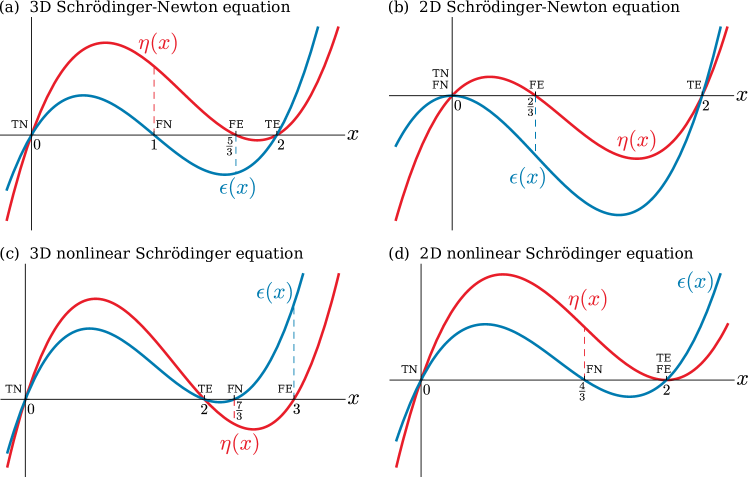
Figure 1: Particle flux $\eta(x)$ (in red) and energy flux $\epsilon(x)$ (in blue) as a function of spectral index $x$ for the limits of the Schrödinger-Helmholtz model. Upper panels for the Schrödinger-Newton model in (a) $d=3$, and (b) in $d=2$. Lower panels for the nonlinear Schrödinger model in (c) $d=3$, and (d) $d=2$. Dashed lines indicate the signs of the fluxes when the spectral index takes the values $x_{\scriptscriptstyle\mathrm{FN}}$ and $x_{\scriptscriptstyle\mathrm{FE}}$.

First we consider the Schrödinger-Newton equations. In both 3D and 2D at the spectral index corresponding to pure energy flux $x_{\scriptscriptstyle\mathrm{FE}}$ we find that $\epsilon$ is negative. On $x_{\scriptscriptstyle\mathrm{FN}}$, the pure particle flux spectrum, we find that $\eta$ is negative in 3D, whereas in 2D there is a degeneracy with the particle equipartition spectrum $x_{\scriptscriptstyle\mathrm{FN}}=x_{\scriptscriptstyle\mathrm{TN}}$ and correspondingly $\eta=0$ there. These findings are in contradiction to the Fjørtoft argument.

For the nonlinear Schrödinger equation in 3D $\epsilon$ is positive at $x_{\scriptscriptstyle\mathrm{FE}}$ and $\eta$ is negative at $x_{\scriptscriptstyle\mathrm{FN}}$. This is in agreement with the Fjørtoft argument. We therefore naively expect that in 3D the Kolmogorov-Zakharov flux cascades are possible. It turns out that the inverse particle Kolmogorov-Zakharov spectrum is realised, with a scale-by-scale transfer of particles to small scales, however the direct energy cascade is nonlocal and the spectrum must be modified to correct a logarithmic divergence in the infrared limit, see refs. (dyachenko1992optical, ; nazarenko2011waveturbbook, ) for details.

For the 2D nonlinear Schrödinger equation the energy flux and equipartition spectra are degenerate $x_{\scriptscriptstyle\mathrm{FE}}=x_{\scriptscriptstyle\mathrm{TE}}$, giving $\epsilon=0$ there, and at the particle flux spectral index $x_{\scriptscriptstyle\mathrm{FN}}$ we find $\eta$ is positive.

These results for the Schrödinger-Newton equations and 2D nonlinear Schrödinger equation are in contradiction to the Fjørtoft argument for a forward energy cascade and inverse particle cascade. However the Fjørtoft argument is robust and predicts that if an initial spectrum evolves, it must push most of the energy towards small scales and particles towards large scales. We therefore conclude that the Schrödinger-Newton Eqs. (3), and the nonlinear Schrödinger Eq. (2) in 2D, do not accomplish this via the Kolmogorov-Zakharov spectra that are determined solely by the values of the flux. To resolve this paradox we develop a simplified theory to reduce the integro-differential kinetic equation to a partial differential equation that is analytically tractable.

II.7 Differential approximation model for wave turbulence

The Kolmogorov-Zakharov solutions of the kinetic equation for the Schrödinger-Newton equations in 3D and 2D, and for the nonlinear Schrödinger equation in 2D, predict the wrong directions for the fluxes as compared to the Fjørtoft argument. Such solutions cannot be realised for any finite scale separation between forcing and dissipation. From experience with other wave turbulence systems we expect that the flux-carrying spectra in these cases are instead close to the zero-flux thermal Rayleigh-Jeans solutions, but with deviations that carry the flux (nazarenko2011waveturbbook, ; PromentOnoratoAsinariNazarenko2012warm, ; connaughton2011mixed, ). These deviations are small deep inside the inertial ranges but become large at the ends, making the spectrum decay rapidly to zero near the dissipation scales. Spectra of this sort are termed “warm” cascades (PromentOnoratoAsinariNazarenko2012warm, ; connaughton2004warm, ; nazarenko2006differential, ; boffetta2009modeling, ). A feature of these solutions is that the thermodynamic potentials $T$ and $\mu$ will be functions of the flux they have to accommodate, and the scales at which the spectrum decays, i.e.,

$$\frac{T}{\mu}=f(\eta,\omega_{\mathrm{min}})$$ (15)

for the inverse cascades and

$$T=g(\epsilon,\omega_{\mathrm{max}})$$ (16)

for direct cascades (nazarenko2011waveturbbook, ; PromentOnoratoAsinariNazarenko2012warm, ; connaughton2011mixed, ), where the functional forms of $f$ and $g$ are to be found, and we have converted from wavenumber to frequency using the dispersion relation $\omega=k^{2}$ (we will continue to refer to “scales” when discussing frequencies as the isotropy of the spectrum allows us to use the dispersion relation to convert between spatial and temporal scales).

To describe warm cascade states we develop a differential approximation model that simplifies the kinetic equation by assuming that interactions are super-local in frequency space ($\omega_{k}\approx\omega_{1}\approx\omega_{2}\approx\omega_{3}$). This allows the collision integral to be reduced to a purely differential operator. Asymptotically-correct stationary solutions of this reduced model can then be found analytically, and these will be qualitatively similar to the solutions for the full kinetic equation (dyachenko1992optical, ; PromentOnoratoAsinariNazarenko2012warm, ; connaughton2011mixed, ; connaughton2004warm, ; nazarenko2006differential, ; boffetta2009modeling, ; LvovNazarenko2006differential, ).

The reduction of the general four-wave kinetic equation to the differential approximation model is done explicitly in Ref. (dyachenko1992optical, ). Here we take a heuristic approach based on the scaling of the kinetic equation and neglect the full calculation of numerical prefactors.

We integrate over angles in $\mathbf{k}$-space and change variables to frequency. The general form of the differential approximation model is then an ordinary differential equation in local conservative form

$$\omega^{d/2-1}\frac{\partial n}{\partial t}=\frac{\partial^{2}R}{\partial\omega^{2}},$$ (17a)

where $$n=n(\omega) \omega$$ is the spectrum expressed as a function of , and the quantity

$$R=S\omega^{\lambda}n^{4}\frac{\partial^{2}}{\partial\omega^{2}}\left(\frac{1}{n}\right)$$ (17b)

is constructed so as to ensure that the Rayleigh-Jeans spectrum is a stationary solution [$\partial_{\omega\omega}(1/n)$ term], the $n^{4}$ term derives from the fact that four-wave interactions are responsible for the spectral evolution, the total $n$ scaling matches the kinetic equation, and $S$ is a constant.

To find $\lambda$ for the systems considered in the present work we examine how the kinetic Eq. (7) scales with $\omega$. Schematically the kinetic equation is

$$\dot{n}=\int\,W^{2}n^{3}\delta(\mathbf{k})\delta(\omega)(\mathrm{d}\mathbf{k})^{3}\sim n^{3}k^{2\beta+2d-2}\sim n^{3}\omega^{\beta+d-1}$$

while the differential approximation (17) scales as

$$\omega^{d/2-1}\dot{n}\sim n^{3}\omega^{\lambda-4}\ .$$

Comparing powers of $\omega$ we find that

$$\lambda=\beta+\frac{3d}{2}+2\ .$$ (18)

II.8 Fluxes in the differential approximation

Comparing Eq. (17a) with (9a) and (9b) we see that the particle and energy fluxes expressed as a function of $\omega$ are, up to a geometrical factor that can be absorbed into $S$,

$$\eta=-\frac{\partial R}{\partial\omega}\qquad\mathrm{and}\qquad\epsilon=-\omega\frac{\partial R}{\partial\omega}+R\ .$$ (19)

respectively.

Putting a power law spectrum $n=\omega^{-x/2}$ into Eqs. (17) and (19) allows us to find expressions for the fluxes. The particle flux is

$$\eta=-\frac{x}{2}\left(\frac{x}{2}-1\right)\left(\beta+\frac{3d}{2}-\frac{3x}{2}\right)S\omega^{\beta+3d/2-3x/2-1}$$

and vanishes when $x=0$ or $x=2$, corresponding to the thermodynamic particle and energy spectral indices of Eqs. (14). The particle flux also vanishes when $x=d+\frac{2\beta}{3}$, corresponding to the energy flux spectral index $x_{\scriptstyle\mathrm{FE}}$ of Eqs. (12a) to (12d). The energy flux is

$$\epsilon=-\frac{x}{2}\left(\frac{x}{2}-1\right)\left(\beta+\frac{3d}{2}-\frac{3x}{2}-1\right)S\omega^{\beta+3d/2-3x/2}$$ (20)

and is again zero for the Rayleigh-Jeans spectra where $x=0$ or $x=2$, and for the constant particle flux (zero energy flux) Kolmogorov-Zakharov spectrum with $x=d+\frac{2\beta}{3}-\frac{2}{3}$.

Thus in the differential approximation model we recover the results of Secs. II.4 and II.5. Furthermore, this model gives a quantitative prediction of $\eta(x)$ and $\epsilon(x)$ for all values of $x$ (to within the limits of the super-local assumption, and the numerical determination of $S$). For example taking $S=1$ and $\omega=1$ we have the cubic functions

$$\eta={} -\frac{x}{2}\left(\frac{x}{2}-1\right)\left(\beta+\frac{3d}{2}-\frac{3x}{2}\right)\,,$$ (21a)

$$\epsilon={} -\frac{x}{2}\left(\frac{x}{2}-1\right)\left(\beta+\frac{3d}{2}-\frac{3x}{2}-1\right)\,,$$ (21b)

that are drawn in Fig. 1, with $\beta=-2$ for the Schrödinger-Newton Eqs. (3) and $\beta=0$ for the nonlinear Schrödinger Eq. (2).

III Turbulent spectra in the Schrödinger-Helmholtz model

III.1 Reconciling with the Fjørtoft argument

Having established the cases in which the Kolmogorov-Zakharov spectra give either the wrong flux directions or zero fluxes for the Schrödinger-Newton and the nonlinear Schrödinger models, we now seek the spectra that give the correct fluxes. To agree with the Fjørtoft argument we require a spectrum for the direct inertial range that carries the constant positive energy flux $\epsilon$ from the forcing scale $\omega_{\mathrm{f}}$ up to the dissipation scale $\omega_{\mathrm{max}}$, but carries no particles. Setting $\eta=\partial_{\omega}R=0$ in eqs. (19) we obtain the ordinary differential equation

$$\epsilon=R=\mathrm{const}>0$$ (22)

in the direct inertial range.

Likewise in the inverse inertial range we require a spectrum that carries the constant negative particle flux $\eta$ from $\omega_{\mathrm{f}}$ to dissipate at $\omega_{\mathrm{min}}$, but carries zero energy. Setting $\epsilon=0$ in Eq. (19) we obtain $\partial_{\omega}R=R/\omega$ and so

$$\eta=-\frac{R}{\omega}=\mathrm{const}<0$$ (23)

in the inverse inertial range.

We now proceed in turn through the 3D and 2D Schrödinger-Newton equations, followed by the 2D nonlinear Schrödinger equation, and use Eqs. (22) and (23) to resolve the predictions from Sec. II.6 that are in conflict with the Fjørtoft argument.

(A full qualitative classification of the single-flux stationary spectra in the differential approximation model for four-wave turbulence is presented in Ref. (grebenev2020dualcascades, ), based on the phase space analysis of an auxiliary dynamical system. Those general results are relevant to the systems under consideration in this paper, however here we will concentrate on the particular functional form of the flux-carrying spectra in the inertial range, and establish the relationships (15), (16) between the thermodynamic potentials and the fluxes, in the spirit of Refs. (nazarenko2011waveturbbook, ; PromentOnoratoAsinariNazarenko2012warm, ; connaughton2011mixed, ).)

III.2 Spectra in the 3D Schrödinger-Newton model

In Sec. II.6 we found that in the 3D Schrödinger-Newton Eqs. (3) both the particle and the energy cascade had the wrong sign on their respective Kolmogorov-Zakharov spectra. We specialise Eq. (18) to this model by setting $\beta=-2$ and $d=3$ and, following Ref. (nazarenko2011waveturbbook, ), we use the ordinary differential Eqs. (22) and (23) to seek warm cascade solutions that carry the fluxes in the directions predicted by Fjørtoft’s argument.

III.2.1 Warm inverse particle cascade in
the 3D Schrödinger-Newton model

The warm cascade is an equilibrium Rayleigh-Jeans spectrum with a small deviation. Thus we propose the spectrum

$$n=\frac{T}{\omega+\mu+\theta(\omega)}$$ (24)

and assume that the disturbance $\theta(\omega)$ is small deep in the inverse inertial range, i.e., $\omega_{\mathrm{min}}\ll\omega\ll\omega_{\mathrm{f}}$. We substitute this into Eqs. (17) and impose the constant-flux condition (23) for the inverse cascade. Linearising with respect to the small disturbance, we obtain the equation

$$\theta^{\prime\prime}(\omega)=-\frac{\eta}{ST^{3}}\frac{(\omega+\mu)^{4}}{\omega^{7/2}}\ .$$

Integrating twice, and noting that $\lvert\eta\rvert$ is negative, yields the following expression for the deviation away from the thermal spectrum that is valid deep in the inertial range

$$\begin{split}\theta(\omega){}=&\frac{\lvert\eta\rvert}{ST^{3}}\left(\frac{4\omega^{5/2}}{15}+\frac{16\mu\omega^{3/2}}{3}\right.\\ &\left.-24\mu^{2}\omega^{1/2}+\frac{16\mu^{3}}{3\omega^{1/2}}+\frac{4\mu^{4}}{15\omega^{3/2}}\right)\,,\end{split}$$ (25)

where we have absorbed the two integration constants by renormalising $T$ and $\mu$.

We can use (25) to obtain a relation between the flux and thermodynamic parameters of the form (15) via the following “approximate matching” argument. We need the warm cascade spectrum to terminate at the dissipation scale $\omega_{\mathrm{min}}$. Therefore near the dissipation scale we expect $\theta(\omega)$ to become significant, compared to the other terms in the denominator of (24), i.e., we expect $\theta(\omega)\sim\omega+\mu$ near $\omega_{\mathrm{min}}$. We put these terms into balance at $\omega_{\mathrm{min}}$ and assume the ordering $\omega_{\mathrm{min}}\ll\mu$. Taking the leading term from Eq. (25), we obtain the flux scaling

$$\left(\frac{T}{\mu}\right)^{3}\sim\frac{4}{15S}\left|\eta\right|\omega_{\mathrm{min}}^{3/2}\ .$$ (26)

Of course this matching procedure is not strictly rigorous as Eq. (25) was derived for small $\theta$ and we are extending it to where $\theta$ is large. Nevertheless, we expect that the scaling relation (26) will give the correct functional relationship between the thermodynamic parameters and the flux and dissipation scale. (Results derived in a similar spirit in other systems give predictions that agree well with direct numerical simulations, see e.g., Ref. (PromentOnoratoAsinariNazarenko2012warm, ).)

Now we examine the structure of the inverse cascade near the dissipation scale. Assuming that the spectrum around $(\omega-\omega_{\mathrm{min}})\ll\omega_{\mathrm{min}}$ is analytic, the condition $n(\omega_{\mathrm{min}})=0$ suggests that the spectrum terminates in a compact front whose leading-order behaviour is of the form $n=A(\omega-\omega_{\mathrm{min}})^{\sigma}$. Again we substitute this ansatz into Eqs. (17), and demand that the flux is carried all the way to the dissipation scale, i.e., we impose the condition (23). Requiring that the flux is frequency independent fixes $A$ and $\sigma$, and we obtain the compact front solution at the dissipation scale

$$n=\left[\frac{9\left|\eta\right|(\omega-\omega_{\mathrm{min}})^{2}}{10S\omega_{\mathrm{min}}^{7/2}}\right]^{1/3}.$$ (27)

We shall find below that the compact front solution is nearly identical near each dissipation range in each model and dimensionality that we examine. This is because the $\sim n^{3}$ scaling of the spectrum in Eqs. (17), and the need for the compact front to vanish at the respective dissipation scale $\omega_{*}$ fixes $\sigma=2/3$. The only difference will be the flux and the power of the respective $\omega_{*}$ in the coefficient, and the sign difference in the power law.

We note that Eq. (25) suggests that $\theta(\omega)$ could again become large at high frequency. Arguing as above, this permits the spectrum to terminate at a compact front at frequency $\omega_{+}>\omega_{\mathrm{min}}$. One could argue likewise for the warm direct energy cascade spectrum, see Eq. (28) below. Indeed all the warm cascade spectra discussed in this paper contain the possibility that they might be bounded by two compact fronts. We discuss this matter in Appendix C.

Using the differential approximation we have shown how the inverse cascade of particles in the 3D Schrödinger-Newton Eqs. (3) is carried by a warm cascade that closely follows a Rayleigh-Jeans spectrum in the inertial range, with a strong deviation near the dissipation scale that gave us an approximate scaling relation between the thermodynamic parameters and the cascade parameters. We also investigated the structure of the spectrum at the dissipation scale and found it to be a compact front with a $\frac{2}{3}$-power law that vanishes at $\omega_{\mathrm{min}}$.

In the rest of this work we will use the same procedures, with the model and dimensionality under consideration giving us the appropriate $\omega$-scaling in the differential approximation, to identify similar features of the cascades. First, we turn to the direct cascade of energy in the 3D Schrödinger-Newton Eqs. (3).

III.2.2 Warm direct energy cascade in the 3D Schrödinger-Newton model

To find a direct cascade of energy for the 3D Schrödinger-Newton equations we again use the warm cascade ansatz (24) and this time impose the constant energy flux condition (22). We go through the same approximate matching procedure as in Sec. III.2.1: we find $\theta(\omega)$ under the assumption that it is small,

$$\begin{split}\theta(\omega){}=&\frac{\epsilon}{ST^{3}}\left(\frac{4\omega^{3/2}}{3}-16\mu\omega^{1/2}\right.\\ &\left.+\frac{8\mu^{2}}{\omega^{1/2}}+\frac{16\mu^{3}}{15\omega^{3/2}}+\frac{4\mu^{4}}{35\omega^{5/2}}\right)\,,\end{split}$$ (28)

where again we have absorbed the two integration constants into $T$ and $\mu$. Extending (28) towards $\omega_{\mathrm{max}}$ where we require it to balance the other terms in the denominator of (24), and assuming $\mu\ll\omega_{\mathrm{max}}$ gives a scaling relation of the type (16)

$$T^{3}\sim\frac{4}{3S}\epsilon\omega_{\mathrm{max}}^{1/2}.$$ (29)

In the immediate vicinity of $\omega_{\mathrm{max}}$ we again expect a compact front. Substituting $n=A(\omega_{\mathrm{max}}-\omega)^{\sigma}$ into (22) gives the leading-order structure

$$n=\left[\frac{9\epsilon(\omega_{\mathrm{max}}-\omega)^{2}}{10S\omega_{\mathrm{max}}^{9/2}}\right]^{1/3}\ .$$ (30)

Again we note that Eq. (28) suggests that $\theta$ can be made large at some low frequency that would lead to a second compact-front cutoff at $\omega_{-}<\omega_{\mathrm{max}}$. All the warm cascade spectra we discuss here have the potential to be terminated at two compact fronts. This is discussed in Appendix C.

III.2.3 Warm dual cascade in the 3D Schrödinger-Newton model

In summary, the results of Secs. III.2.1 and III.2.2 predict that for the 3D Schrödinger-Newton model in the forced-dissipative setup, the movement of particles to large scales and energy to small scales is realised by a dual warm cascade spectrum. This spectrum starts close to the Rayleigh-Jeans distribution (13) near the forcing scale $\omega_{\mathrm{f}}$ and then deviates strongly away, until it vanishes at compact 2/3 power-law fronts at the dissipation scales $\omega_{\mathrm{min}}$ and $\omega_{\mathrm{max}}$.

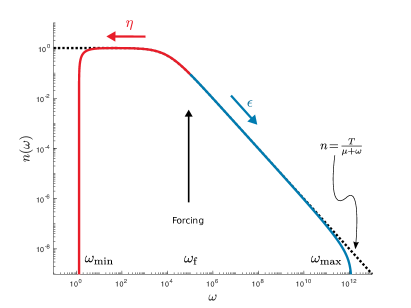
Figure 2: Dual warm cascade in the 3D Schrödinger-Newton equations. The inverse particle cascade, with negative particle flux $\eta$, is shown in red. In blue is the direct energy cascade with positive flux $\epsilon$. The black dashed line is the thermodynamic equipartition spectrum (13). (See main text for parameters.)

We show the dual warm cascade in Fig. 2, which was obtained by numerically integrating Eq. (22) forwards and Eq. (23) backwards from the initial condition that the spectrum and its derivative matched the Rayleigh-Jeans spectrum (13) at $\omega_{\mathrm{f}}=10^{5}$, with $T=\mu=10^{4}$. The warm cascades carry a particle flux $\eta=-3.75$ to large scales and energy flux $\epsilon=\omega_{\mathrm{f}}^{2}\lvert\eta\rvert$ to small scales, and the geometric constant $S=1$.

The dual warm cascade for the 2D Schrödinger-Newton and 2D nonlinear Schrödinger models can be obtained in a similar fashion. They are qualitatively similar to Fig. 2 so we omit displaying them.

III.3 Spectra in the 2D Schrödinger-Newton model

Now we turn to the 2D Schrödinger-Newton Eqs. (3), setting $\beta=-2$ and $d=2$ in Eq. (18). In Sec. II.6 we found that the particle equipartition and cascade spectra coincided, making the particle flux zero, and that the energy flux had the wrong sign.

III.3.1 Log-corrected inverse particle cascade in the 2D Schrödinger-Newton model

The degeneracy between the particle Rayleigh-Jeans and Kolmogorov-Zakharov spectra $n\sim\omega^{0}$ can be lifted by making a logarithmic correction to this spectrum. Substituting the trial solution $n=B\ln^{z}\!\left(\omega/\omega_{\mathrm{min}}\right)$ into Eqs. (17) and enforcing constant negative particle flux (23) that is independent of $\omega$ gives

$$n=\left[\frac{3\left|\eta\right|}{S}\ln\!\left(\frac{\omega}{\omega_{\mathrm{min}}}\right)\right]^{1/3}$$ (31)

to leading order deep in the inverse inertial range.

To find a relation between the thermodynamic parameters and the cascade parameters we carry out the approximate matching procedure described in Sec. III.2.1 at low frequency $\omega\sim\omega_{\mathrm{min}}\ll\mu$, obtaining

$$\left(\frac{T}{\mu}\right)^{3}\sim\frac{\left|\eta\right|}{S}\ln\omega_{\mathrm{min}}.$$ (32)

As $\omega\to\omega_{\mathrm{min}}$ the spectrum in Eq. (31) becomes zero, as we would expect given $\omega_{\mathrm{min}}$ is a dissipation scale. However we note that this is only a qualitative statement as subleading terms will start to dominate in this limit, meaning that Eq. (31) is no longer the correct stationary spectrum there. To obtain the correct leading-order structure near $\omega_{\mathrm{min}}$ we look for a compact front solution and find once again a $2/3$ power law,

$$n=\left[\frac{9\left|\eta\right|(\omega-\omega_{\mathrm{min}})^{2}}{10S\omega_{\mathrm{min}}^{2}}\right]^{1/3}.$$ (33)

III.3.2 Warm direct energy cascade in the 2D Schrödinger-Newton model

To find a forward energy cascade for the 2D Schrödinger-Newton model we again look for a warm cascade, substituting Eq. (24) into (17) and seeking a constant energy flux (22). Solving for the perturbation and matching the deviation to the other terms in the denominator in (24) at $\omega\sim\omega_{\mathrm{max}}\gg\mu$ gives the scaling relation

$$T^{3}\sim\frac{\epsilon\omega_{\mathrm{max}}^{2}}{6S}.$$

The compact front near $\omega_{\mathrm{max}}$ has leading-order form

$$n=\left[\frac{9\epsilon(\omega_{\mathrm{max}}-\omega)^{2}}{10S\omega_{\mathrm{max}}^{3}}\right]^{1/3}.$$ (34)

III.4 Spectra in the 2D nonlinear Schrödinger model

In Sec. II.6 we found that the Kolmogorov-Zakharov particle flux spectrum for the nonlinear Schrödinger model was positive rather than negative, and that the Kolmogorov-Zakharov energy flux spectrum coincides with the Rayleigh-Jeans energy equipartition spectrum. We specialise to the 2D nonlinear Schrödinger Eq. (2) by setting $\beta=0$ and $d=2$ in Eq. (18) and take these issues in turn. (These results recapitulate and extend the discussion in Chapter 15 of Ref. (nazarenko2011waveturbbook, ).)

III.4.1 Warm inverse particle cascade in the 2D nonlinear Schrödinger model

The approximate matching procedure described above gives the scaling relation

$$\left(\frac{T}{\mu}\right)^{3}\sim\frac{\left|\eta\right|}{6S\omega_{\mathrm{min}}^{2}}$$

for the inverse cascade. The compact front solution at the dissipation scale has the structure

$$n=\left[\frac{9\left|\eta\right|(\omega-\omega_{\mathrm{min}})^{2}}{10S\omega_{\mathrm{min}}^{4}}\right]^{1/3}.$$ (35)

III.4.2 Log-corrected direct energy cascade in the 2D nonlinear Schrödinger model

The degeneracy of $n\propto\omega^{-1}$ corresponding to both the Kolmogorov-Zakharov energy flux spectrum and the Rayleigh-Jeans energy equipartition spectrum can be again lifted by making a logarithmic correction. Substituting the spectrum $n=(B/\omega)\ln^{z}\!\left(\omega_{\mathrm{max}}/\omega\right)$ into Eqs. (17) and imposing Eq. (22) we obtain

$$n=\frac{1}{\omega}\left[\frac{3\epsilon\ln(\omega_{\mathrm{max}}/\omega)}{S}\right]^{1/3}\ .$$ (36)

Comparing Eq. (36) to the energy equipartition spectrum $n=T/\omega$ we have a relation of the kind in Eq. (16), namely

$$T^{3}\sim\frac{3\epsilon}{S}\ln\omega_{\mathrm{max}}.$$ (37)

We obtain the same scaling [apart from the factor of 3 on the right-hand side of Eq. (37)] if we assume a warm cascade and carry out the approximate matching procedure as described in Sec. III.2.1. This is natural as the log-corrected solution (36) is of a prescribed form whereas in the warm cascade argument the perturbation $\theta$ is not constrained from the outset, so the two solutions are two different perturbations from the thermal spectrum. However by continuity they should give the same scaling of thermal with cascade parameters, differing only by an $\mathcal{O}(1)$ constant.

As in Sec. III.3.1 the log-corrected spectrum (36) becomes zero at the dissipation scale. However the structure will not be correct here as sub-leading terms would start to become significant. The correct leading-order structure for the front is again the $2/3$ power-law

$$n=\left[\frac{9\epsilon(\omega_{\mathrm{max}}-\omega)^{2}}{10S\omega_{\mathrm{max}}^{5}}\right]^{1/3}\ .$$

III.5 Crossover from warm to Kolmogorov-Zakharov cascade in the 3D Schrödinger-Helmholtz model

As mentioned in Sec. II.6 the dual cascade in the 3D nonlinear Schrödinger limit of (1) is achieved by a scale-invariant Kolmogorov-Zakharov spectrum, rather than the warm cascade discussed in Sec. III.2 for the 3D Schrödinger-Newton limit. Both these two regimes may be accessed if the removal of waveaction from the weakly nonlinear wave content of the system (through dissipation or absorption into the condensate) is situated at larger scales than the cosmological constant which controls the crossover between the two limits of Eqs. (1), i.e., if $\omega_{\mathrm{min}}\ll\Lambda$. We sketch this schematically in Fig. 3(a) when $\omega_{\mathrm{f}}\gg\Lambda$, so the crossover from the Kolmogorov-Zakharov to the warm cascade happens in the inverse inertial range, and in Fig. 3(b) when $\omega_{\mathrm{f}}\ll\Lambda$ and the crossover happens in the direct inertial range.

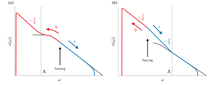
Figure 3: Sketch of the crossover from a warm cascade [which follows closely the thermodynamic spectrum (13) shown in black dashes] to a scale-free cascade, the latter with the Kolmogorov-Zakharov spectral indices shown, in the 3D Schrödinger-Helmholtz equations. The crossover happens around $\omega\approx\Lambda$, with the warm cascade in $\omega\gg\Lambda$ and the Kolmogorov-Zakharov cascade in $\omega\ll\Lambda$. Depending on placement of the forcing scale the crossover happens (a) in the inverse cascade (shown in red) or (b) in the direct cascade (shown in blue).

Note that Fig. 3 is a sketch and not produced directly by using the stationary differential approximation model (19). This is because in the crossover regime $\omega\approx\Lambda$ the interaction coefficient (5d) cannot be put into scale-invariant form. Accurate realisations of Fig. 3 must await direct numerical simulation of Eqs. (1) in future work.

The crossover from a scale-invariant cascade dominated by flux to an equipartition-like spectrum at small scales is common in turbulence, when a flux-dominated spectrum runs into a scale where the flux stagnates and thermalises. The stagnation is due to a mismatch of flux rate between the scale-invariant spectrum and the small-scale processes, whether that be (hyper-)dissipation in hydrodynamic turbulence (connaughton2004warm, ; frisch2008hyperviscosity, ), or a different physical regime such as the crossover from hydrodynamic to Kelvin wave turbulence in superfluids (lvov2007bottlenecksuperfluid, ). Our case here, the crossover from the nonlinear Schrödinger to the Schrödinger-Newton regime, is more like the latter but again the details await further work.

IV Conclusion and outlook

IV.1 Summary and discussion of results

In this work we have developed the theory of weak wave turbulence in the Schrödinger-Helmholtz Eqs. (1), which contain as limits both the nonlinear Schrödinger and Schrödinger-Newton Eqs. (2) and (3). We obtained the kinetic equation for the Schrödinger-Helmholtz model in the case of four-wave turbulence, that is of random fluctuations of the field with no condensate present, and we used the Fjørtoft argument to predict the dual cascade of particles upscale and energy downscale in this model.

Using the differential approximation of the full kinetic equation, we have characterised the statistically steady states of its Schrödinger-Newton and nonlinear Schrödinger limits in the case of a forced-dissipated system. We found that the dual cascade is achieved via a warm spectrum for the Schrödinger-Newton limit in 2D and 3D, and for the nonlinear Schrödinger limit in 2D. For the 3D nonlinear Schrödinger limit the Kolmogorov-Zakharov spectra are responsible for the cascades, and we have schematically illustrated the crossover between the warm and Kolmogorov-Zakharov cascades when both limits of the full Schrödinger-Helmholtz model are accessible.

Finally we found scaling relationships between the thermodynamic parameters and the fluxes and dissipation scales of the type (15) and (16) for these cascades. We have thus characterised the processes by which particles are condensed at the largest scales, and energy sent to small scales, in both limits of the Schrödinger-Helmholtz model. The results for the nonlinear Schrödinger model have appeared in the literature before, but the results for the Schrödinger-Newton model are new and are relevant to the problem of cosmological structure formation in a fuzzy dark matter universe, and to optical systems where nonlocal effects are significant.

For the bulk of this work we considered an open system where forcing matched dissipation. This allowed us to discuss the stationary warm spectra that will realise the dual cascade in the forced-dissipated system. There remains the question of how the dual cascade will be realised in the time-dependent case where turbulence evolves from an initial condition; such a case is far more relevant when discussing the formation of galaxies, and realistic protocols in an optics experiment. Experience with other wave turbulence systems shows that time-dependent cascades are strongly controlled by the capacity of the relevant flux spectra, defined as follows. We consider pushing the dissipation scales towards the extremes $k_{\mathrm{min}}\to 0$ and $k_{\mathrm{max}}\to\infty$. If in this extremal case the integral defining an invariant, cf. (8), converges (or diverges) at the limit towards which that invariant is cascading, then the spectrum is said to have finite (infinite) capacity, respectively. It has been observed elsewhere that for finite capacity systems the cascading invariant fills out the inertial range in the wake of a self-similar front that reaches the dissipation scale in finite time, even in the extremal case, and then reflects back towards the forcing scale, with the Kolmogorov-Zakharov flux spectrum established behind the returning front. By contrast for infinite capacity systems the front takes infinite time to establish in the extremal case (semikoz1995kinetics, ; semikoz1997condensation, ; galtier2000weak, ).

For the small and large-scale limits of the Schrödinger-Helmholtz equations we have found that the flux-carrying spectra are the Rayleigh-Jeans-like warm spectra, except for the nonlinear Schrödinger limit in 3D where they are Kolmogorov-Zakharov spectra. It is easy to check that for all these cases, the inverse particle cascade has finite capacity and the direct cascade has infinite capacity. We therefore expect that in an evolving system the inverse cascade will resemble the stationary spectra we have discussed, and that these spectra will be established in finite time, but will have parameters ($\mu$ and $T$ in the warm case) that vary with time. As for the direct cascade, for an unforced system there is always a $k_{\mathrm{max}}$ sufficiently remote that the energy in any initial condition is insufficient to fill the cascade spectrum. Therefore we do not expect that the direct energy cascade spectrum will be realised generically in systems evolving according to (1), although we might expect to see the cascade when $k_{\mathrm{max}}$ is small enough, and the initial condition contains enough energy to act as a reservoir with which to fill the cascade spectrum.

Our hypotheses above regarding the time-evolving case are in broad agreement with numerical results in the recent study of the 3D Schrödinger-Newton equations by Levkov et al. (levkov2018gravitational, ). They show by direct numerical simulation that, starting from a statistically homogeneous random field, the formation of coherent structures is preceded by a kinetic evolution, after which the structures become inhomogeneous due to a gravitational Jeans instability (the latter collapsed structures are what they call a condensate and the condensation time they report is the time of collapse, terminology we shall adhere to while comparing our study to theirs). Moreover, they argue that this kinetic evolution is governed not by pure flux spectra of Kolmogorov-Zakharov type, but rather by a process of thermalisation. Their conclusion entirely agrees with the scenario of large-scale structure formation via a warm cascade, but the theory we have developed in this work suggests an explanation that is different from the interpretation given in (levkov2018gravitational, ).

First, we can quantitatively demonstrate agreement between the wave turbulence theory of this paper and the numerics of Ref. (levkov2018gravitational, ) by estimating the characteristic timescale $\tau_{\mathrm{kin}}\sim N/\lvert\mathrm{Coll}[n_{\mathbf{k}}]\rvert$ over which Eq. (7) acts, where $N$ is a typical value of the spectrum and $\mathrm{Coll}[n_{\mathbf{k}}]$ is the right-hand side of (7), whose size is estimated in Appendix B, Eq. (48). Taking values from the Gaussian initial spectrum of (levkov2018gravitational, ) we obtain a characteristic kinetic timescale of $\tau_{\mathrm{kin}}\sim$4.3\text{\times}{10}^{5}\text{\,}$$ in dimensionless units. This compares favourably to the condensation timescale of $1.08\text{\times}{10}^{6}\text{\,}$ reported in (levkov2018gravitational, ) for this initial condition: large-scale homogeneous structure forms over a timescale of roughly $2\tau_{\mathrm{kin}}$ before a gravitational instability collapses this structure into a compact object. This lends credence to our kinetic equation capturing the essence of the condensation processes examined by Levkov et al. Furthermore they give timescale estimates for kinetic condensation in dimensional units for two models of self-gravitating bosons, which links our results to astrophysically relevant processes.

The points of difference between this study and Ref. (levkov2018gravitational, ) lie in the nature of the kinetic equations that are used in each. Levkov et al. derive a Landau-type differential kinetic equation by assuming that only boson-boson interactions that are strongly nonlocal in physical space contribute to the dynamics, which leads to small-amplitude scattering, an assumption that becomes more accurate at higher energies. They also imply that the lack of Kolmogorov-Zakharov cascades is due to the nonlocality of the system. By contrast our kinetic equation is derived without restriction to strong nonlocality, and is valid at arbitrary energies. Importantly, we attribute the lack of Kolmogorov-Zakharov cascades to the fact that they give the wrong flux directions, rather than the effects of nonlocality.

Additionally, when we reduce our kinetic equation (7) to the differential approximation model (17), the latter is explicitly constructed to keep the general Rayleigh-Jeans spectrum (13) as a stationary solution. However the only thermodynamic spectrum that solves the differential kinetic equation in Ref. (levkov2018gravitational, ) is the energy equipartition spectrum: (13) with $\mu=0$. The low-energy part of the general Rayleigh-Jeans spectrum is excluded from their solution, yet we argue that this is the part responsible for the dynamical inverse cascade of particles that builds large-scale structure. Despite this, at the condensation time Levkov et al. observe excellent agreement between the spectrum obtained by direct numerical simulation of (3), the spectrum obtained by evolving their kinetic equation, and the low-energy part of the energy equipartition spectrum.

The agreement with the energy equipartition spectrum at the condensation time we explain by noting that $\mu=0$ is indeed the criterion for condensation in the local Eq. (2) (connaughton2005condensation, ), and the arguments are sufficiently general that this criterion should apply universally. As mentioned above, we conjecture that the time-evolving spectra might be Rayleigh-Jeans-like, with time-dependent thermodynamic parameters. As the system evolves towards the condensation time we expect to see $\mu(t)$ shrink $0$, leaving only the energy equipartition spectrum at the condensation time, as observed in (levkov2018gravitational, ). The deviation of the observed spectrum from the thermodynamic one at high energies might be related to the infinite capacity of the direct warm cascade spectrum, meaning that the cascade may have had insufficient time to fill out at the highest frequencies, as mentioned above. Indeed Levkov et al. make reference to this part of the spectrum having a slow thermalisation timescale.

Thus, we summarise that our kinetic equation and its differential approximation is more general than that of Ref. (levkov2018gravitational, ), in terms of not being restricted to highly nonlocal interactions, and containing the general Rayleigh-Jeans spectrum that could explain more features of the evolution in the four-wave kinetic regime. Clearly further work is needed to explore and test these hypotheses.

IV.2 Outlook for wave turbulence in Schrödinger-Helmholtz systems

We now speculate on what further perspectives wave turbulence could bring to the astrophysical and optical systems to which Eqs. (1) apply. Focusing first on the astrophysical application, our results suggest that the first process that starts to accumulate a condensate of dark matter particles at large scales in the early universe is an unsteady weakly nonlinear evolution that bears the hallmark of a warm dual cascade. Following this initial phase of condensation the subsequent evolution would follow the same broad lines as has already been documented in the literature, namely that gravitational collapse into a collection of virialised 3D spheroidal haloes will ensue (levkov2018gravitational, ; mocz2019first, ).

We also conjecture that wave turbulence may have much to say regarding certain other details that have already been noted. For example, the structure of haloes has been reported as a solitonic core that is free of turbulence surrounded by a turbulent envelope (mocz2017galaxyI, ). The exclusion of turbulence from the core is reminiscent of the externally trapped defocusing nonlinear Schrödinger Eq. (2), where wave turbulence combined with wavepacket (Wentzel-Kramers-Brillouin) analysis predicts the refraction of Bogoliubov sound waves towards the edges of the condensate, where transition from the three-wave Bogoliubov wave turbulence to four-wave processes could occur (lvov2003wave, ). On the other hand the virialisation of haloes suggests a condition of critical balance where the linear propagation and nonlinear interaction timescales of waves are equal scale by scale. In that case the weak wave turbulence described here is not applicable and new spectral relations must be found based on the critical balance hypothesis (nazarenko2011waveturbbook, ; nazarenko2011critical, ).

After the formation of haloes the next step of the evolution will be their mutual interaction. As mentioned in Sec. I.3, in nonlinear optics experiments and simulation of Eqs. (3) in one dimension (with six-wave interactions taken into account to break the integrability of the system), it has been observed that a random field creates a condensate via the dual cascade, which then collapses into solitons. These solitons then interact via the exchange of waves and finally merge into one giant soliton that dominates the dynamics (LaurieEtAl2012_1DOpticalWT, ; BortolozzoEtAl2009_OpticalWTCondensnLight, ). It seems plausible that the same phenomenology might carry over to the Schrödinger-Helmholtz equations, and into higher spatial dimensions.

Indeed, in cosmological simulations of binary and multiple halo collisions, scattering events, inelastic collisions, and mergers are all observed (mocz2017galaxyI, ; bernal2006scalar, ; schwabe2016simulations, ; amin2019formation, ). Following such events, subsequent virialisation of the products involves ejection of some of the mass of the haloes (guzman2004evolution, ; guzman2006gravcooling, ). A detailed study of these processes should consider both the weakly nonlinear wave component and the strongly nonlinear haloes, and how the two components interact. Numerical studies could obtain effective collision kernels for those interactions in order to develop a kinetic equation for the “gas” of haloes that results from the collapse of a condensate. We note that work has been done in this spirit in Ref. (amin2019formation, ) but without detailed consideration of the wave component. In our opinion it is crucial to incorporate wave turbulence into the study of the Schrödinger-Helmholtz model to uncover the full richness of the behaviour that this system manifests.

Finally, we expect that all the processes outlined above in the 3D astrophysical case—condensation via the dual cascade, fragmentation by modulational instability, soliton formation, and soliton interaction/merger via the exchange of weakly nonlinear waves—will be qualitatively the same in 2D. This makes them all amenable to direct observation by nonlocal nonlinear optics experiments. As mentioned in Sec. I.2.2 theoretical (navarrete2017spatial, ; paredes2020optics, ) and experimental (Faccio2016_OpticalNewtSchro, ; Beckenstein2015_OpticalNewtSchro, ) comparisons have been made between astrophysical phenomena and experiments in thermo-optic media. To observe the wave turbulence cycle of condensation, collapse, and soliton interaction that we describe here one could also look to using nematic liquid crystals and modifying the one-dimensional experiments of (LaurieEtAl2012_1DOpticalWT, ; BortolozzoEtAl2009_OpticalWTCondensnLight, ) to 2D. Any such experiment would need to have fine control over losses and nonlinearity strength in order to keep within the wave turbulence regime while the condensate is being built up. Liquid crystals are an attractive optical medium in this respect due to several inherently tunable parameters (ferreira2018superfluidity, ) that would assist in achieving conditions relevant to wave turbulence studies.

Appendix A Relation between the cosmological constant and the Jeans swindle

In Sec. I.2.3 we motivated the inclusion of a local term in Eq. (1b) in the dark matter application as representing a cosmological constant (kiessling2003jeans, ), and asserted that this is equivalent to using the “Jeans swindle”. In this Appendix we expand on this statement.

Eq. (3b) is well-posed for spatially infinite domains in which the support of $\rho(\mathbf{x})=\lvert\psi(\mathbf{x})\rvert^{2}$ is compact, but if one seeks an equilibrium with spatially-constant $V$ and $\rho$ the only solution is the trivial null solution (an empty domain). The Jeans swindle (BinneyTremaine1987_GalacDynBook, ) is the ad hoc replacement of $V$ in Eq. (3a) with $\tilde{V}$ that solves $\nabla^{2}\tilde{V}=\gamma\tilde{\rho}$, where the tildes refer to fluctuations of quantities about a nonzero equilibrium, whose existence is entirely paradoxical. In a periodic domain $\Omega=\mathbb{T}^{d}_{L}$ of side $L$ the equivalent problem is that Eq. (3b) can only be satisfied when $\Omega$ is empty, as can be seen by integrating over $\Omega$, and using the divergence theorem and the periodic boundary conditions. The Jeans swindle is then implemented by replacing (3b) with

$$\nabla^{2}\tilde{V}=\gamma\left(\rho-\langle\rho\rangle_{\Omega}\right)$$ (38)

where the box average of the number density $\langle\rho\rangle_{\Omega}=L^{-d}\int_{\Omega}\rho\,\mathrm{d}\mathbf{x}$ is the equilibrium solution, and one solves only for $\tilde{V}$.

It is shown in Ref. (kiessling2003jeans, ) in the infinite-domain case that the Jeans swindle can formally be justified by considering the Helmholtz-like Eq. (1b) instead of Eq. (3b), as the former is well-posed without the restriction of the right-hand side needing to integrate to zero, and then taking the limit $\Lambda\to 0$. For the case of the periodic boundary we simply note that averaging (1b) gives $\langle V\rangle_{\Omega}=-\gamma\langle\rho\rangle_{\Omega}/\Lambda$. Substitution back into (1b) and writing $V=\tilde{V}+\langle V\rangle_{\Omega}$ recovers Eq. (38) in the limit $\Lambda\to 0$.

Appendix B Wave turbulence in inhomogeneous systems

In the main body of this paper we have applied the theory of weak wave turbulence to the Schrödinger-Helmholtz system, and described the initial stage of wave condensation via the dual cascade in a forced-dissipated setup. Crucial to this analysis is the assumption that the system is statistically spatially homogeneous, as only then can the dynamical variables, such as the spectrum and linear frequency, be characterised solely by time or axial distance $t$ and wavenumber $\mathbf{k}$. However for inhomogeneous systems these quantities may vary with spatial position $\mathbf{x}$. This brings into play physical effects that are not present in homogeneous systems and that are described by a different dynamical equation. In this Appendix we discuss the extension of wave turbulence theory to inhomogeneous systems and make simple estimates of the conditions under which the processes outlined in this paper will be the dominant dynamical processes.

To take into account inhomogeneities of the wave field we define a local spectrum that can now vary with spatial position, with characteristic spatial scale $D$, via the Wigner transform of the $\psi(\mathbf{x},t)$ field (alber1978effects, ):

$$n_{\mathbf{k}}(\mathbf{x},t)=\int\!\langle\psi(\mathbf{x}-\mathbf{y}/2,t)\,\psi^{*}\!(\mathbf{x}+\mathbf{y}/2,t)\rangle e^{-i\mathbf{y}\cdot\mathbf{k}}\,d\mathbf{y}\,.$$ (39)

Let $K$ be a characteristic wavenumber associated with the spectrum. If $DK\gg 1$ a Wentzel-Kramers-Brillouin analysis gives the following Vlasov-like equation of motion for the local spectrum (see, e.g., (alber1978effects, ; zakharov1985hamiltonian, ; dyachenko1992wave-vortex, ; lvov1977spatially, ; hall2002statistical, ; onorato2003landau, ; picozzi2007towards, ; levkov2018gravitational, )):

$$\frac{\partial n_{\mathbf{k}}}{\partial t}+\nabla_{\!\mathbf{k}}\tilde{\omega}_{\mathbf{k}}\cdot\nabla_{\!\mathbf{x}}n_{\mathbf{k}}-\nabla_{\!\mathbf{x}}\tilde{\omega}_{\mathbf{k}}\cdot\nabla_{\!\mathbf{k}}n_{\mathbf{k}}=\mathrm{Coll[n_{\mathbf{k}}]}\,.$$ (40)

The term $\mathrm{Coll}[n_{\mathbf{k}}]$ on the right-hand side of Eq. (40) is the collision integral of the wave kinetic equation (7) which describes spectral evolution via nonlinear wave interactions.

The left-hand side of (40) is the Liouville operator describing the motion of wavepackets through phase $(\mathbf{k},\mathbf{x})$ space, in which trajectories are given by Hamilton’s equations. The latter are $\partial_{t}\mathbf{x}=\nabla_{\!\mathbf{k}}\tilde{\omega}_{\mathbf{k}}$ and $\partial_{t}\mathbf{k}=-\nabla_{\!\mathbf{x}}\tilde{\omega}_{\mathbf{k}}$, where the effective Hamiltonian is the renormalised dispersion relation $\tilde{\omega}_{\mathbf{k}}$ which, as we shall shortly discuss, is a function of the local spectrum. If the collision integral vanishes, wavepackets move ballistically in phase space in a manner that conserves waveaction. As they move across the inhomogeneous wave field, e.g., through a turbulent patch, the amplitude of the spectrum changes and therefore $\tilde{\omega}_{\mathbf{k}}$ changes. In this manner wavepackets can be distorted as they move, leading to a redistribution of the spectrum and an exchange of energy between the wavepackets and the background turbulence (zakharov1985hamiltonian, ; dyachenko1992wave-vortex, ; hall2002statistical, ; onorato2003landau, ).

The distortion of wavepackets brings about two effects: either wavepackets are dispersed [second term on the left-hand side of (40), noting that $\nabla_{\!\mathbf{k}}\tilde{\omega}_{\mathbf{k}}=\mathbf{v}_{\mathrm{g}}$, the group velocity], or in the case of a focusing nonlinearity such as the gravitational one considered in this paper, the wavepacket can become unstable and bunch up in physical space (third term). As we justify below, these collapsing events are an incoherent version of the monochromatic modulational instability, and lead to the formation of compact strongly-nonlinear structures, studied in deep water gravity waves in Ref. (onorato2003landau, ), and in 1D local (hall2002statistical, ) and nonlocal optical turbulence (picozzi2011incoherent, ). These collapses were also observed in the 3D Schrödinger-Newton equations in their dark matter context (levkov2018gravitational, ), after a period of evolution governed by four-wave kinetics, such as we describe in the main body of this paper (see Sec. IV.1). It is thus important to distinguish when processes associated with inhomogeneity will occur faster than processes due to four-wave interaction. Below we derive conditions to evaluate which of these two types of processes dominate the dynamics.

B.0.1 Renormalised dispersion relation

For any nonlinear equation with even-wave interactions of the type $M\leftrightarrow M$, such as the Schrödinger-Helmholtz equations (of type $2\leftrightarrow 2$), the linear dispersion relation $\omega_{\mathbf{k}}$ is modified by the nonlinearity (nazarenko2011waveturbbook, ). This can be seen in Eq. (5c)where the diagonal terms in the nonlinear Hamiltonian give a contribution whose effect is to shift the linear frequency by $\omega_{\scriptscriptstyle\mathrm{NL}}$, i.e., the dispersion relation is renormalised to

$$\tilde{\omega}_{\mathbf{k}}=\omega_{\mathbf{k}}+\omega_{\scriptscriptstyle\mathrm{NL}}\,.$$

This frequency shift is the leading effect of the nonlinearity, and does not lead to interaction between wave modes.

For the Schrödinger-Helmholtz equations the nonlinear frequency correction is

$$\omega_{\scriptscriptstyle\mathrm{NL}}(\mathbf{k})=-\gamma\sum_{\mathbf{k}_{1}}\left(\frac{1}{\lvert\mathbf{k}-\mathbf{k}_{1}\rvert^{2}+\Lambda}+\frac{1}{\Lambda}\right)\lvert\psi_{1}\rvert^{2}$$ (41)

and depends on both $\mathbf{k}$ and the spectrum. When the spectrum is spatially dependent, as in (39), then the renormalised frequency also varies in space, leading to the distortion of wavepackets described above.

We can conveniently estimate the size of $\omega_{\scriptscriptstyle\mathrm{NL}}$ in the case of weak inhomogeneity $DK\gg 1$. Then in physical space Eq. (41) is replaced by

$$\omega_{\scriptscriptstyle\mathrm{NL}}(\mathbf{x},t)=-\gamma\int\!G_{\ell_{*}}\!(\mathbf{x}-\mathbf{y})\mathcal{N}(\mathbf{y},t)\,d\mathbf{y}$$ (42)

(picozzi2007towards, ), where $\mathcal{N}(\mathbf{x},t)=(2\pi)^{-d}\int\!n_{\mathbf{k}}(\mathbf{x},t)\,d\mathbf{k}=\langle\lvert\psi(\mathbf{x},t)\rvert^{2}\rangle$ is the average local level of fluctuations, whose typical amplitude we denote $N$. Here $G_{\ell_{*}}\!(\mathbf{x}-\mathbf{y})$ is the Green’s function for Eq. (1b). It is useful to extract the explicit dependence on $\ell_{*}=1/\sqrt{\Lambda}$ by the scaling space as $\mathbf{x}=\ell_{*}\bm{\xi}$ and defining $G(\bm{\xi})$ as the normalised Green’s function satisfying $(\nabla^{2}_{\bm{\xi}}-1)G(\bm{\xi})=\delta^{(d)}(\bm{\xi})$, and that integrates to unity. Doing so we find $G(\bm{\xi})=\ell_{*}^{d-2}G_{\ell_{*}}(\mathbf{x})$. (For self-consistency, passing to the local limit requires that $\tilde{\gamma}=\gamma\ell_{*}^{2}\to\mathrm{const}$.) We approximate the convolution in (42) by multiplying the average fluctuation level $N$ with the volume of the $d$-ball of size $\ell_{*}$. Neglecting geometrical factors and the sign we obtain

$$\omega_{\scriptscriptstyle\mathrm{NL}}\sim 2\gamma\ell_{*}^{2}N.$$ (43)

For $l_{*}K\ll 1$ Eq. (41) reduces to the well-known value for the nonlinear Schrödinger equation $-2\tilde{\gamma}\sum_{\mathbf{k}}\langle\lvert\psi_{\mathbf{k}}\rvert^{2}\rangle$, so the estimate in (43) becomes exact.

We now provide estimates on the various terms in Eq. (40) in order to determine when the wavepacket collapse due to inhomogeneity will dominate over either dispersion, or four-wave nonlinear interactions.

B.1 Incoherent modulational instability

We assume an isotropic spectrum that has spectral width $\Delta K$ about the representative wavenumber $K$. Thus, in terms of the measure of the average fluctuations $N$ and neglecting geometric factors, the spectrum can be estimated as

$$n_{\mathbf{k}}\sim\frac{N}{K^{d-1}\Delta K}\,.$$ (44)

With estimates (43) and (44) we can estimate the sizes of the second and third terms on the left-hand side of (40). The second term describes the dispersion of wavepackets, which is a stabilising process. Noting that the linear frequency $\omega_{\mathbf{k}}=k^{2}$, that $\omega_{\scriptscriptstyle\mathrm{NL}}$ is $\mathbf{k}$-independent, and that the inhomogeneity of the spectrum has characteristic size $D$, we estimate

$$\nabla_{\!\mathbf{k}}\tilde{\omega}_{\mathbf{k}}\cdot\nabla_{\!\mathbf{x}}n_{\mathbf{k}}\sim\frac{N}{DK^{d-2}\Delta K}\,.$$ (45)

Turning to the focusing term, we note that $\nabla_{\!\mathbf{x}}\tilde{\omega}_{\mathbf{k}}=\nabla_{\!\mathbf{x}}\omega_{\scriptscriptstyle\mathrm{NL}}$ as the linear frequency is $\mathbf{x}$-independent. The spectrum varies over length $D$, however the convolution in (42) “smears out” the variations of the spectrum over the length $\ell_{*}$, meaning that $\omega_{\scriptscriptstyle\mathrm{NL}}$ will vary over a length $\max(D,\ell_{*})$. Additionally the spectrum has a $\mathbf{k}$-space width of $\Delta K$ by assumption, so we can approximate the gradient in $\nabla_{\!\mathbf{k}}n_{\mathbf{k}}$ by $1/\Delta K$. Bringing these considerations together, we estimate the focusing term as

$$\nabla_{\!\mathbf{x}}\tilde{\omega}_{\mathbf{k}}\cdot\nabla_{\!\mathbf{k}}n_{\mathbf{k}}\sim\frac{\gamma\ell_{*}^{2}N^{2}}{\max(D,\ell_{*})K^{d-1}(\Delta K)^{2}}\,.$$ (46)

Comparing (45) and (46) we find that wavepacket collapse into incoherent solitons is favoured over wave dispersion when

$$\frac{D}{\max(D,\ell_{*})}\frac{\tilde{\gamma}N}{K\Delta K}>1\,.$$ (47)

To justify the assertion that these collapse events are the result of an incoherent modulational, (or Benjamin-Feir) instability, we note that the latter has been extensively studied in the 1D local nonlinear Schrödinger equation, for example in the context of extreme ocean waves (onorato2013rogue, ). In the oceanic literature an important dimensionless number has been identified that controls the tendency for polychromatic wavepackets to destabilise and form strongly nonlinear structures such as rogue waves: the Benjamin-Feir Index (BFI) (onorato2003landau, ; janssen2003nonlinear, ). In the notation we have established in this Appendix, this is

$$BFI=\sqrt{\frac{\tilde{\gamma}N}{K^{2}}}\,,$$

with the modulational instability triggering the formation of nonlinear structures when $BFI>1$ (janssen2003nonlinear, ). However our condition (47) for inhomogenity on scales greater than the nonlocality length ($D>\ell_{*}$) and with a spectrum whose width is of the same order as the characteristic wavenumber ($\Delta K\sim K$) is just $BFI^{2}>1$ for wavepacket collapse. Thus we conclude that the ratio on the left-hand side of (47) contains the same physics as the BFI, so we identify the third term in Eq. (40) with modulational instability and wavepacket collapse. Note that (47) is valid for both local and nonlocal nonlinearities, indicating that our condition is a generalisation of the BFI to the nonlocal case, and for the spectra of arbitrary width $\Delta K$.

B.2 Kinetic regime

The derivation of the wave kinetic equation requires that the nonlinearity is small in the original equation of motion. Quantitatively this means that the linear wave period is much smaller than the characteristic timescale for nonlinear evolution (nazarenko2011waveturbbook, ), or in other words $\lvert\omega_{\mathbf{k}}n_{\mathbf{k}}\rvert\gg\lvert\mathrm{Coll}[n_{\mathbf{k}}]\rvert$. We estimate the collision integral as

$$\mathrm{Coll}[n_{\mathbf{k}}]\sim\frac{\gamma^{2}N^{3}}{(K^{2}+1/\ell_{*}^{2})^{2}K^{d+2}}\,,$$ (48)

giving the first condition for wave turbulence

$$(\gamma N)^{2}\ll\frac{(K^{2}+1/\ell_{*}^{2})^{2}K^{5}}{\Delta K}\,.$$ (49)

In inhomogeneous domains, wave turbulence processes will only dominate if in Eq. (40) the collision integral is larger than the focusing term that leads to wavepacket collapse, i.e., $\lvert\mathrm{Coll}[n_{\mathbf{k}}]\rvert>\lvert\nabla_{\!\mathbf{x}}\tilde{\omega}_{\mathbf{k}}\cdot\nabla_{\!\mathbf{k}}n_{\mathbf{k}}\rvert$. This gives a second condition for wave turbulence when the kinetic regime dominates over wavepacket collapse:

$$\frac{1}{\max(D,\ell_{*})}\frac{\ell_{*}^{2}(K^{2}+1/\ell_{*}^{2})^{2}K^{3}}{\gamma N(\Delta K)^{2}}<1\,.$$ (50)

We now examine what our conditions (47), (49) and (50) imply about the applicability of the kinetic regime.

B.2.1 Kinetic regime in the local limit

For Eq. (40) to be valid, and for the nonlinearity to be local, we have $D\gg 1/K\gg\ell_{*}$. In this limit, condition (49) becomes $(\tilde{\gamma}N)^{2}\ll K^{5}/\Delta K$, and the condition for the modulational instability to be stable [i.e., (47) with the ordering reversed] is $\tilde{\gamma}N<K(\Delta K)$. If the spectrum is broad ($\Delta K\sim K$) then the conditions for weak nonlinearity and modulational stability become identical, $(\tilde{\gamma}N)^{2}\ll K^{4}$, which agrees with the physical intuition that for weak wave turbulence processes one must not have the spectrum collapsing into strongly nonlinear objects.

In the local limit condition (50) becomes $K^{3}/D(\Delta K)^{2}<\tilde{\gamma}N$. Thus for wave turbulence to be the dominant process the nonlinearity must satisfy the double inequality

$$\frac{K^{3}}{D(\Delta K)^{2}}<\tilde{\gamma}N<\min\!\left(K(\Delta K),\frac{K^{5/2}}{(\Delta K)^{1/2}}\right)\,.$$ (51)

These inequalities are violated when either the spectrum is too narrow, or the inhomogeneity length is too short. If $\Delta K$ is small then no matter how large $D$ is, the system is still vulnerable to modulational instability via the first term on the right-hand side of (51), and if the spectrum is broad but $D\to 1/K$ the system again becomes modulationally unstable from the left-hand side of (51), as both sides of the inequality approach the same value.

We thus conclude that wave turbulence in the Schrödinger-Helmholtz equations in their local limit requires that the spectrum is sufficiently broad everywhere, and that the inhomogeneity length of the spectrum is sufficiently long.

B.2.2 Kinetic regime in the nonlocal limit

Validity of (40) and a nonlocal nonlinearity both require $D,\ell_{*}\gg 1/K$. We now consider the ordering $\ell_{*}\sim D$ or $\ell_{*}\gg D$. These give $K^{6}/(\Delta K)^{2}\ll\gamma N$ for condition (50), whereas condition (49) becomes $(\gamma N)^{2}\ll K^{9}/\Delta K$. For a broad spectrum this means that $\gamma N$ is both much smaller and much greater than $K^{8}$, which is impossible (the violation of the inequalities is worse for a narrow spectrum).

We conclude that nonlocal wave turbulence is not possible when $\ell_{*}\sim D$ or $\ell_{*}\gg D$. Instead, The ordering $D\gg\ell_{*}\gg 1/K$ allows for wave turbulence for sufficiently large $D$.

Appendix C Bimodal cascade spectra in the differential approximation model

In Sec. III.2 we noted that Eqs. (25) and (28) permitted the deviation away from the Rayleigh-Jeans spectrum $\theta(\omega)$ to become large at both low and high frequencies for both the inverse and direct cascades. This led to the intriguing possibility that we could have a warm inverse cascade spectrum, which carries only particles, arising from the cutoff at $\omega_{+}$, becoming large at intermediate $\omega$ and terminating at the cutoff at $\omega_{\mathrm{min}}$. Similarly one could imagine that the warm direct cascade of energy might exist between $\omega_{-}$ and $\omega_{\mathrm{max}}$, terminating at compact fronts at those frequencies. For both of these to be realised the combined spectrum would have two maxima. The frequency where the two cascades met would then be the forcing scale, i.e., $\omega_{\mathrm{f}}=\omega_{+}=\omega_{-}$, and the forcing would be such that all the particles were swept upscale and the energy downscale with the spectrum at $\omega_{\mathrm{f}}$ vanishing. This scenario is illustrated in Fig. 4.

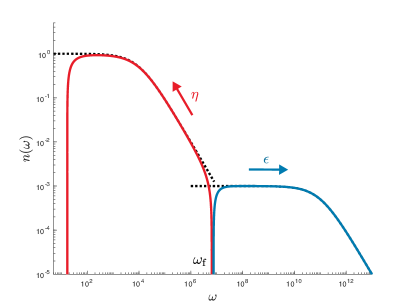
Figure 4: Double-peaked spectra representing a solution of the differential approximation model where particles are swept upscale (red curve) and energy downscale (blue curve) from forcing at $\omega_{\mathrm{f}}$ at a zero value for the spectrum. Black dashed lines represent the two different thermodynamic spectra that match the middle of the two peaks of the spectrum. For parameters see main text.

[To obtain the direct cascade, shown in blue in Fig. 4, we have integrated (22) forwards to $\omega_{\mathrm{max}}$ and backwards to $\omega_{-}$ from a spectrum and its derivative matching Eq. (13) at $\omega=10^{12}$ with $T=10^{8}$ and $\mu=10^{11}$. Likewise to obtain the inverse cascade shown in red, we integrated (23) backwards to $\omega_{\mathrm{min}}$ and forwards to $\omega_{+}$ from a spectrum and its derivative matching Eq. (13) at $\omega=10^{5}$ with $T=\mu=10^{4}$. The fluxes were $\eta=-150$ and $\epsilon=\omega_{\mathrm{f}}^{2}\lvert\eta\rvert$ with $\omega_{\mathrm{f}}\approx\omega_{-}\approx\omega_{+}=6.44\times 10^{6}$. In Fig. 4 we have chosen parameters to slightly separate $\omega_{-}$ and $\omega_{+}$ for clarity.]

We argue here that this scenario, although technically possible within the differential approximation, is implausible for more realistic models like the wave kinetic equation (7) or the original dynamical equation itself [the Schrödinger-Helmholtz system (1) or its limits]. Note that this possibility is common to all the warm cascade spectra we discuss here. Following on from Sec. III.2 we take the concrete example of the Schrödinger-Newton model in 3D, but similar arguments can be made for either the Schrödinger-Newton model or nonlinear Schrödinger model in 2D. The argument proceeds by seeking compatibility with wide inertial ranges, $\omega_{\mathrm{min}}\ll\omega_{+}$ for the inverse cascade and $\omega_{-}\ll\omega_{\mathrm{max}}$ for the direct cascade.

First considering the inverse particle cascade, Eq. (25) and the requirement that there exists a range of $\omega>\omega_{\mathrm{min}}$ for which $\theta(\omega)$ is small, gives the ordering $\omega_{\mathrm{min}}\ll\mu$. This ordering gave the relation (26) between flux and thermodynamic parameters. Now, a cutoff at $\omega_{+}$ implies that in that vicinity the deviation must become comparable to the other terms in the denominator of the warm spectrum (24). We set $\theta(\omega_{+})\sim\mu+\omega_{+}$ here. If we then let either $\omega_{+}\sim\mu$ or $\omega_{+}\ll\mu$ and substitute (26) then we obtain $\omega_{+}\sim\omega_{\mathrm{min}}$, which is not compatible with a wide inertial range. A scale separation between forcing and dissipation is only possible if the we have the ordering $\omega_{\mathrm{min}}\ll\mu\ll\omega_{+}$ for the inverse cascade.

Next we consider the direct energy cascade. Eq. (28) for the deviation, and the requirement that it must be small for some $\omega<\omega_{\mathrm{max}}$ gives the ordering $\mu\ll\omega_{\mathrm{max}}$. From this we obtained the relation (29). If we have a low-frequency cutoff at $\omega_{-}$ then near there it must match the other terms in the denominator of (24). We set $\theta(\omega_{-})\sim\mu+\omega_{-}$ and consider $\omega_{-}\sim\mu$ and $\omega_{-}\gg\mu$. Substituting (29) gives $\omega_{-}\sim\omega_{\mathrm{max}}$ for these two cases, which is not compatible with a wide inertial range. Therefore for the direct cascade we must have $\omega_{-}\ll\mu\ll\omega_{\mathrm{max}}$.

Thus if we seek a double-peaked “flux-sweeping” spectrum with the inverse and direct warm cascades joining at $\omega_{\mathrm{f}}$ and the spectrum being zero there, then the cascades could not share the same thermodynamic parameters, as $\mu$ must lie deep within the inertial ranges of both cascades. Indeed, to realise such a spectrum in Fig. 4 we have had to choose very different sets of thermodynamic parameters for each inertial range. This is technically possible within the differential approximation, as each steady cascade is described by a second order ordinary differential Eq. (22) or Eq. (23), which only requires for its solution the value of the spectrum and its derivative at the forcing scale.

However when considering a fuller model one must consider a more realistic forcing protocol, for example in simulations setting the spectrum to be drawn from a particular distribution at a certain level in a narrow range around $\omega_{\mathrm{f}}$ at each timestep. This sets the amplitude and derivative of the spectrum at the forcing scale at the same prescribed value for both cascades, corresponding to prescription of the thermodynamic parameters $T$ and $\mu$ that both cascades share. It is therefore hard to imagine a scenario of forcing which could realise the double-peaked spectrum in a more realistic model like Eqs. (1) or Eq. (7). For example the four-wave collision integral in Eq. (7) has the effect of smoothing out irregularities in the spectrum, and so we expect that any stationary solution will be at least continuous and differentiable. In this respect, this discussion stands as a cautionary example that the differential approximation includes exotic solutions like the double-peaked spectrum of Fig. 4, that a more physically relevant model would not permit.

- [1] Vladimir E. Zakharov, Victor S. L’vov, and Gregory Falkovich. Kolmogorov spectra of turbulence I: Wave turbulence. Springer Series in Nonlinear Dynamics. Springer, 1992.
- [2] Sergey Nazarenko. Wave turbulence, volume 825 of Lecture Notes in Physics. Springer, 2011.
- [3] Lev Pitaevskii and Sandro Stringari. Bose-Einstein Condensation and Superfluidity, volume 164 of International series of monographs on physics. Oxford University Press, 2016.
- [4] E. P. Gross. Structure of a quantized vortex in boson systems. Il Nuovo Cimento, 20(3):454–477, 1961.
- [5] Lev P. Pitaevskii. Vortex lines in an imperfect Bose gas. Sov. Phys. JETP, 13(2):451–454, 1961.
- [6] A. C. Newell and J. V. Moloney. Nonlinear Optics. ATIMS Series. Addison-Wesley, Redwood City, CA, 1992.
- [7] Robert W. Boyd. Nonlinear optics. Academic press, 3 edition, 2008.
- [8] G. B. Whitham. Linear and Nonlinear Waves, volume 42 of Pure and Applied Mathematics: A Wiley-Interscience Series of Texts, Monographs and Tracts. John Wiley & Sons, New York, 1999.
- [9] David J. E. Marsh. Axion cosmology. Phys. Rep., 643:1–79, 2016.
- [10] Jens C. Niemeyer. Small-scale structure of fuzzy and axion-like dark matter. Prog. Part. Nucl. Phys., 113:103787, 2020.
- [11] Wayne Hu, Rennan Barkana, and Andrei Gruzinov. Fuzzy cold dark matter: The wave properties of ultralight particles. Phys. Rev. Lett., 85(6):1158–1161, 2000.
- [12] Abril Suárez, Victor H. Robles, and Tonatiuh Matos. A review on the scalar field/Bose-Einstein condensate dark matter model. In Claudia Moreno González, José Edgar Madriz Aguilar, and Luz Marina Reyes Barrera, editors, Accelerated Cosmic Expansion, pages 107–142, Cham, 2014. Springer International Publishing.
- [13] Pierre-Henri Chavanis. Self-gravitating Bose-Einstein Condensates. In Xavier Calmet, editor, Quantum Aspects of Black Holes, chapter 6, pages 151–194. Springer International Publishing, Cham, 2015.
- [14] Lam Hui, Jeremiah P. Ostriker, Scott Tremaine, and Edward Witten. Ultralight scalars as cosmological dark matter. Phys. Rev. D, 95(4):043541, 2017.
- [15] Elisa G. M. Ferreira. Ultra-light dark matter. arXiv preprint arXiv:2005.03254, 2020.
- [16] M. R. Baldeschi, G. B. Gelmini, and R. Ruffini. On massive fermions and bosons in galactic halos. Phys. Lett. B, 122(3-4):221–224, 1983.
- [17] Jae-weon Lee and In-gyu Koh. Galactic halos as boson stars. Phys. Rev. D, 53(4):2236–2239, 1996.
- [18] Hsi-Yu Schive, Tzihong Chiueh, and Tom Broadhurst. Cosmic structure as the quantum interference of a coherent dark wave. Nat. Phys., 10(7):496–499, 2014.
- [19] Akhilesh Kumar Verma, Rahul Pandit, and Marc E. Brachet. The formation of compact objects at finite temperatures in a dark-matter-candidate self-gravitating bosonic system. arXiv preprint arXiv:1912.10172, 2019.
- [20] J. M. Overduin and P. S. Wesson. Dark matter and background light. Phys. Rep., 402:267–406, 2004.
- [21] P. J. E. Peebles and Bharat Ratra. The cosmological constant and dark energy. Rev. Mod. Phys., 75(2):559–606, 2003.
- [22] Volker Springel, Simon D. M. White, Adrian Jenkins, Carlos S. Frenk, Naoki Yoshida, Liang Gao, Julio Navarro, Robert Thacker, Darren Croton, John Helly, et al. Simulations of the formation, evolution and clustering of galaxies and quasars. Nature, 435(7042):629–636, 2005.
- [23] D. H. Weinberg, J. S. Bullock, F. Governato, R. Kuzio de Naray, and Peter A. H. G. Cold dark matter: Controversies on small scales. Proc. Natl. Acad. Sci. U. S. A., 112(40):12249–12255, 2015.
- [24] James S. Bullock and Michael Boylan-Kolchin. Small-scale challenges to the CDM paradigm. Annu. Rev. Astron. Astrophys, 55:343–387, 2017.
- [25] T. Harko. Bose-Einstein condensation of dark matter solves the core/cusp problem. J. Cosmol. Astropart. Phys., 2011(05):022, 2011.
- [26] David J. E. Marsh and Ana-Roxana Pop. Axion dark matter, solitons and the cusp–core problem. Mon. Not. R. Astron. Soc., 451(3):2479–2492, 2015.
- [27] Monica Colpi, Stuart L. Shapiro, and Ira Wasserman. Boson stars: Gravitational equilibria of self-interacting scalar fields. Phys. Rev. Lett., 57(20):2485–2488, 1986.
- [28] Philip Mocz, Mark Vogelsberger, Victor H. Robles, Jesús Zavala, Michael Boylan-Kolchin, Anastasia Fialkov, and Lars Hernquist. Galaxy formation with BECDM—I. Turbulence and relaxation of idealized haloes. Mon. Not. R. Astron. Soc., 471(4):4559–4570, 2017.
- [29] Philip Mocz, Anastasia Fialkov, Mark Vogelsberger, Fernando Becerra, Mustafa A. Amin, Sownak Bose, Michael Boylan-Kolchin, Pierre-Henri Chavanis, Lars Hernquist, Lachlan Lancaster, et al. First star-forming structures in fuzzy cosmic filaments. Phys. Rev. Lett., 123(14):141301, 2019.
- [30] Philip Mocz, Anastasia Fialkov, Mark Vogelsberger, Fernando Becerra, Xuejian Shen, Victor H. Robles, Mustafa A. Amin, Jesús Zavala, Michael Boylan-Kolchin, Sownak Bose, Federico Marinacci, Pierre-Henri Chavanis, Lachlan Lancaster, and Lars Hernquist. Galaxy formation with BECDM—II. Cosmic filaments and first galaxies. Mon. Not. R. Astron. Soc., 494(2):2027–2044, 04 2020.
- [31] M. D. Iturbe Castillo, J. J. Sánchez-Mondragón, and S. Stepanov. Formation of steady-state cylindrical thermal lenses in dark stripes. Opt. Lett., 21(20):1622–1624, 1996.
- [32] Iam-Choon Khoo. Liquid Crystals. John Wiley & Sons, 2 edition, 2007.
- [33] Allan W. Snyder and D. John Mitchell. Accessible solitons. Science, 276(5318):1538–1541, 1997.
- [34] Claudio Conti, Marco Peccianti, and Gaetano Assanto. Route to nonlocality and observation of accessible solitons. Phys. Rev. Lett., 91(7):073901, 2003.
- [35] Carmel Rotschild, Oren Cohen, Ofer Manela, Mordechai Segev, and Tal Carmon. Solitons in nonlinear media with an infinite range of nonlocality: first observation of coherent elliptic solitons and of vortex-ring solitons. Phys. Rev. Lett., 95(21):213904, 2005.
- [36] Carmel Rotschild, Barak Alfassi, Oren Cohen, and Mordechai Segev. Long-range interactions between optical solitons. Nat. Phys., 2(11):769–774, 2006.
- [37] Víctor M. Pérez-García, Vladimir V. Konotop, and Juan J. García-Ripoll. Dynamics of quasicollapse in nonlinear schrödinger systems with nonlocal interactions. Phys. Rev. E, 62(3):4300, 2000.
- [38] Ole Bang, Wieslaw Krolikowski, John Wyller, and Jens Juul Rasmussen. Collapse arrest and soliton stabilization in nonlocal nonlinear media. Phys. Rev. E, 66(4):046619, 2002.
- [39] Marco Peccianti, Claudio Conti, and Gaetano Assanto. Optical modulational instability in a nonlocal medium. Phys. Rev. E, 68(2):025602, 2003.
- [40] Neda Ghofraniha, Claudio Conti, Giancarlo Ruocco, and Stefano Trillo. Shocks in nonlocal media. Phy. Rev. Lett., 99(4):043903, 2007.
- [41] G. Xu, D. Vocke, D. Faccio, J. Garnier, Thomas Roger, Stefano Trillo, and A. Picozzi. From coherent shocklets to giant collective incoherent shock waves in nonlocal turbulent flows. Nat. Commun., 6(1):8131, 2015.
- [42] Thomas Roger, Calum Maitland, Kali Wilson, Niclas Westerberg, David Vocke, Ewan M. Wright, and Daniele Faccio. Optical analogues of the Newton-Schrödinger equation and boson star evolution. Nat. Commun., 7:13492, 2016.
- [43] Rivka Bekenstein, Ran Schley, Maor Mutzafi, Carmel Rotschild, and Mordechai Segev. Optical simulations of gravitational effects in the Newton-Schrödinger system. Nat. Phys., 11:872–878, 2015.
- [44] Alvaro Navarrete, Angel Paredes, José R Salgueiro, and Humberto Michinel. Spatial solitons in thermo-optical media from the nonlinear Schrödinger-Poisson equation and dark-matter analogs. Phys. Rev. A, 95(1):013844, 2017.
- [45] Angel Paredes, David N Olivieri, and Humberto Michinel. From optics to dark matter: A review on nonlinear Schrödinger–Poisson systems. Phys. D, 403:132301, 2020.
- [46] Michael K.-H. Kiessling. The “Jeans swindle”: a true story — mathematically speaking. Adv. Appl. Math., 31(1):132–149, 2003.
- [47] James Binney and Scott Tremaine. Galactic Dynamics. Princeton Series in Astrophysics. Princeton University Press, 2 edition, 2008.
- [48] W. F. Vinen and J. J. Niemela. Quantum turbulence. J. Low Temp. Phys., 128(5):167–231, 2002.
- [49] Carlo F. Barenghi, Russell J. Donnelly, and W. F. Vinen. Quantized Vortex Dynamics and Superfluid Turbulence, volume 571 of Lecture Notes in Physics. Springer-Verlag, 2001.
- [50] Michikazu Kobayashi and Makoto Tsubota. Quantum turbulence in a trapped Bose-Einstein condensate. Physical Review A, 76(4):045603, 2007.
- [51] Giorgio Krstulovic and Marc Brachet. Dispersive bottleneck delaying thermalization of turbulent bose-einstein condensates. Phys. Rev. Lett., 106(11):115303, 2011.
- [52] Marios C. Tsatsos, Pedro E. S. Tavares, André Cidrim, Amilson R. Fritsch, Mônica A. Caracanhas, F. Ednilson A. dos Santos, Carlo F. Barenghi, and Vanderlei S. Bagnato. Quantum turbulence in trapped atomic Bose-Einstein condensates. Phys. Rep., 622:1–52, 2016.
- [53] Makoto Tsubota, Kazuya Fujimoto, and Satoshi Yui. Numerical Studies of Quantum Turbulence. J. Low Temp. Phys., 188(5-6):119–189, 2017.
- [54] Nicolás P. Müller, Marc-Etienne Brachet, Alexandros Alexakis, and Pablo D. Mininni. Abrupt transition between three-dimensional and two-dimensional quantum turbulence. Phys. Rev. Lett., 124(13):134501, 2020.
- [55] Jason Laurie, Umberto Bortolozzo, Sergey Nazarenko, and Stefania Residori. One-dimensional optical wave turbulence: Experiment and theory. Phys. Rep., 514(4):121–175, 2012.
- [56] S. Dyachenko, A. C. Newell, A. Pushkarev, and V. E. Zakharov. Optical turbulence: weak turbulence, condensates and collapsing filaments in the nonlinear Schrödinger equation. Phys. D, 57(1):96–160, 1992.
- [57] A. Picozzi, J. Garnier, T. Hansson, P. Suret, S. Randoux, G. Millot, and D. N. Christodoulides. Optical wave turbulence: Towards a unified nonequilibrium thermodynamic formulation of statistical nonlinear optics. Phys. Rep., 542(1):1–132, 2014.
- [58] Catherine Sulem and Pierre-Louis Sulem. The Nonlinear Schrödinger Equation: Self-Focusing and Wave Collapse, volume 139 of Applied Mathematical Sciences. Springer-Verlag, New York, 1999.
- [59] Victor S. L’vov and Sergey Nazarenko. Weak turbulence of Kelvin waves in superfluid He. Low Temp. Phys., 36(8-9):785–791, 2010.
- [60] Umberto Bortolozzo, Jason Laurie, Sergey Nazarenko, and Stefania Residori. Optical wave turbulence and the condensation of light. J. Opt. Soc. Am. B, 26(12):2280–2284, 2009.
- [61] D. G. Levkov, A. G. Panin, and I. I. Tkachev. Gravitational Bose-Einstein condensation in the kinetic regime. Phys. Rev. Lett., 121(15):151301, 2018.
- [62] Yeontaek Choi, Yuri V. Lvov, and Sergey Nazarenko. Probability densities and preservation of randomness in wave turbulence. Phys. Lett. A, 332(3-4):230–238, 2004.
- [63] Yeontaek Choi, Yuri V. Lvov, and Sergey Nazarenko. Joint statistics of amplitudes and phases in wave turbulence. Phys. D, 201(1-2):121–149, 2005.
- [64] Yeontaek Choi, Yuri V. Lvov, and Sergey Nazarenko. Wave turbulence. In Recent developments in fluid dynamics, page 225, Kepala, India, 2004. Transworld Research Network.
- [65] Ragnar Fjørtoft. On the changes in the spectral distribution of kinetic energy for two-dimensional, nondivergent flow. Tellus, 5(3):225–230, 1953.
- [66] Yuri Lvov, Sergey Nazarenko, and Robert West. Wave turbulence in Bose-Einstein condensates. Phys. D, 184(1-4):333–351, 2003.
- [67] A.N. Kolmogorov. The local structure of turbulence in incompressible viscous fluid for very large Reynolds numbers. Proc. R. Soc. Lond. A, 434:9–13, 1991.
- [68] Colm Connaughton, Sergey Nazarenko, and Alan C. Newell. Dimensional analysis and weak turbulence. Phys. D, 184(1-4):86–97, 2003.
- [69] Davide Proment, Miguel Onorato, Pietro Asinari, and Sergey Nazarenko. Warm cascade states in a forced-dissipated Boltzmann gas of hard spheres. Phys. D, 241(5):600–615, 2012.
- [70] Colm Connaughton and Rachel McAdams. Mixed flux-equipartition solutions of a diffusion model of nonlinear cascades. Europhys. Lett. EPL, 95(2):24005, 2011.
- [71] Colm Connaughton and Sergey Nazarenko. Warm cascades and anomalous scaling in a diffusion model of turbulence. Phys. Rev. Lett., 92(4):044501, 2004.
- [72] Sergey Nazarenko. Differential approximation for Kelvin wave turbulence. JETP Lett., 83(5):198–200, 2006.
- [73] G. Boffetta, A. Celani, D. Dezzani, J. Laurie, and S. Nazarenko. Modeling Kelvin wave cascades in superfluid helium. J. Low Temp. Phys., 156(3-6):193–214, 2009.
- [74] V. S. L’vov and S. Nazarenko. Differential model for 2D turbulence. JETP Lett., 83(12):541–545, 2006.
- [75] V. N. Grebenev, S. B. Medvedev, S. V. Nazarenko, and B. V. Semisalov. Steady states in dual-cascade wave turbulence. J. Phys. A, 53(36):365701, 2020.
- [76] Uriel Frisch, Susan Kurien, Rahul Pandit, Walter Pauls, Samriddhi Sankar Ray, Achim Wirth, and Jian-Zhou Zhu. Hyperviscosity, Galerkin truncation, and bottlenecks in turbulence. Phys. Rev. Lett., 101(14):144501, 2008.
- [77] Victor S. L’vov, Sergei V. Nazarenko, and Oleksii Rudenko. Bottleneck crossover between classical and quantum superfluid turbulence. Phys. Rev. B, 76(2):024520, 2007.
- [78] D. V. Semikoz and I. I. Tkachev. Kinetics of Bose condensation. Phys. Rev. Lett., 74(16):3093–3097, 1995.
- [79] D. V. Semikoz and I. I. Tkachev. Condensation of bosons in the kinetic regime. Phys. Rev. D, 55(2):489–502, 1997.
- [80] S. Galtier, S. V. Nazarenko, Alan C. Newell, and A. Pouquet. A weak turbulence theory for incompressible magnetohydrodynamics. J. Plasma Phys., 63(5):447–488, 2000.
- [81] Colm Connaughton, Christophe Josserand, Antonio Picozzi, Yves Pomeau, and Sergio Rica. Condensation of classical nonlinear waves. Phys. Rev. Lett., 95(26):263901, 2005.
- [82] Sergei V. Nazarenko and Alexander A. Schekochihin. Critical balance in magnetohydrodynamic, rotating and stratified turbulence: towards a universal scaling conjecture. J. of Fluid Mech., 677:134–153, 2011.
- [83] Argelia Bernal and F Siddhartha Guzmán. Scalar field dark matter: Head-on interaction between two structures. Phys. Rev. D, 74(10):103002, 2006.
- [84] Bodo Schwabe, Jens C. Niemeyer, and Jan F. Engels. Simulations of solitonic core mergers in ultralight axion dark matter cosmologies. Phys. Rev. D, 94(4):043513, 2016.
- [85] Mustafa A. Amin and Philip Mocz. Formation, gravitational clustering, and interactions of nonrelativistic solitons in an expanding universe. Phys. Rev. D, 100(6):063507, 2019.
- [86] F. Siddhartha Guzmán and L. Arturo Ureña-López. Evolution of the Schrödinger-Newton system for a self-gravitating scalar field. Phys. Rev. D, 69(12):124033, 2004.
- [87] F. Siddhartha Guzmán and L. Arturo Ureña-López. Gravitational cooling of self-gravitating Bose condensates. Astrophys. J., 645(2):814–819, 2006.
- [88] Tiago D. Ferreira, Nuno A. Silva, and A. Guerreiro. Superfluidity of light in nematic liquid crystals. Phys. Rev. A, 98(2):023825, 2018.
- [89] I. E. Alber. The effects of randomness on the stability of two-dimensional surface wavetrains. Proc. R. Soc. London, Ser. A, 363(1715):525–546, 1978.
- [90] V. E. Zakharov, S. L. Musher, and A. M. Rubenchik. Hamiltonian approach to the description of non-linear plasma phenomena. Phys. Rep., 129(5):285–366, 1985.
- [91] A. I. Dyachenko, S. V. Nazarenko, and V. E. Zakharov. Wave-vortex dynamics in drift and -plane turbulence. Phys. Lett. A, 165(4):330–334, 1992.
- [92] V. S. Lvov and A. M. Rubenchik. Spatially non-uniform singular weak turbulence spectra. Soviet Physics-JETP, 45(1):67–74, 1977.
- [93] B. Hall, M. Lisak, D. Anderson, R. Fedele, and V. E. Semenov. Statistical theory for incoherent light propagation in nonlinear media. Phys. Rev. E, 65(3):035602, 2002.
- [94] Miguel Onorato, Alfred Osborne, Renato Fedele, and Marina Serio. Landau damping and coherent structures in narrow-banded 1 + 1 deep water gravity waves. Phys. Rev. E, 67(4):046305, 2003.
- [95] Antonio Picozzi. Towards a nonequilibrium thermodynamic description of incoherent nonlinear optics. Opt. Express, 15(14):9063–9083, 2007.
- [96] A. Picozzi and J. Garnier. Incoherent soliton turbulence in nonlocal nonlinear media. Phys. Rev. Lett., 107(23):233901, 2011.
- [97] M. Onorato, S. Residori, U. Bortolozzo, A. Montina, and F. T. Arecchi. Rogue waves and their generating mechanisms in different physical contexts. Phys. Rep., 528(2):47–89, 2013.
- [98] P. A. E. M. Janssen. Nonlinear four-wave interactions and freak waves. J. Phys. Oceanogr., 33(4):863–884, 2003.