A weight-dependent local correlation density-functional approximation for ensembles

Abstract

We report a local, weight-dependent correlation density-functional approximation that incorporates information about both ground and excited states in the context of density-functional theory for ensembles (eDFT). This density-functional approximation for ensembles is specially designed for the computation of single and double excitations within Gross–Oliveira–Kohn (GOK) DFT (i.e., eDFT for neutral excitations), and can be seen as a natural extension of the ubiquitous local-density approximation in the context of ensembles. The resulting density-functional approximation, based on both finite and infinite uniform electron gas models, automatically incorporates the infamous derivative discontinuity contributions to the excitation energies through its explicit ensemble weight dependence. Its accuracy is illustrated by computing single and double excitations in one-dimensional many-electron systems in the weak, intermediate and strong correlation regimes. Although the present weight-dependent functional has been specifically designed for one-dimensional systems, the methodology proposed here is general, i.e., directly applicable to the construction of weight-dependent functionals for realistic three-dimensional systems, such as molecules and solids.

I Introduction

Over the last two decades, density-functional theory (DFT) Hohenberg and Kohn (1964); Kohn and Sham (1965); Parr and Yang (1989) has become the method of choice for modeling the electronic structure of large molecular systems and materials. The main reason is that, within DFT, the quantum contributions to the electronic repulsion energy — the so-called exchange-correlation (xc) energy — is rewritten as a functional of the electron density $n\equiv n(\boldsymbol{r})$, the latter being a much simpler quantity than the many-electron wave function. The complexity of the many-body problem is then transferred to the xc density functional. Despite its success, the standard Kohn-Sham (KS) formulation of DFT Kohn and Sham (1965) (KS-DFT) suffers, in practice, from various deficiencies. Woodcock, Schaefer, and Schreiner (2002); Tozer (2003); Tozer et al. (1999); Dreuw, Weisman, and Head-Gordon (2003); Sobolewski and Domcke (2003); Dreuw and Head-Gordon (2004); Tozer and Handy (1998, 2000); Casida et al. (1998); Casida and Salahub (2000); Tapavicza et al. (2008); Levine et al. (2006) The description of strongly multiconfigurational ground states (often referred to as “strong correlation problem”) still remains a challenge. Gori-Giorgi and Seidl (2010); Fromager (2015); Gagliardi et al. (2017) Another issue, which is partly connected to the previous one, is the description of low-lying quasi-degenerate states.

The standard approach for modeling excited states in a DFT framework is linear-response time-dependent DFT (TDDFT). Runge and Gross (1984); Casida (1995); Casida and Huix-Rotllant (2012) In this case, the electronic spectrum relies on the (unperturbed) pure-ground-state KS picture, which may break down when electron correlation is strong. Moreover, in exact TDDFT, the xc energy is in fact an xc action Vignale (2008) which is a functional of the time-dependent density $n\equiv n(\boldsymbol{r}_{,}t)$ and, as such, it should incorporate memory effects. Standard implementations of TDDFT rely on the adiabatic approximation where these effects are neglected. Dreuw and Head-Gordon (2005) In other words, the xc functional is assumed to be local in time. Casida (1995); Casida and Huix-Rotllant (2012) As a result, double electronic excitations (where two electrons are simultaneously promoted by a single photon) are completely absent from the TDDFT spectrum, thus reducing further the applicability of TDDFT. Maitra et al. (2004); Cave et al. (2004); Mazur and Włodarczyk (2009); Romaniello et al. (2009); Sangalli et al. (2011); Mazur et al. (2011); Huix-Rotllant et al. (2011); Elliott et al. (2011); Maitra (2012); Sundstrom and Head-Gordon (2014); Loos et al. (2019)

When affordable (i.e., for relatively small molecules), time-independent state-averaged wave function methods B. O. Roos et al. (1996); Andersson et al. (1990); Angeli, Cimiraglia, and Malrieu (2001); Angeli et al. (2001); Angeli, Cimiraglia, and Malrieu (2002); Helgaker, Jørgensen, and Olsen (2013) can be employed to fix the various issues mentioned above. The basic idea is to describe a finite (canonical) ensemble of ground and excited states altogether, i.e., with the same set of orbitals. Interestingly, a similar approach exists in DFT. Referred to as Gross–Oliveira–Kohn (GOK) DFT, Gross, Oliveira, and Kohn (1988a, b); Oliveira, Gross, and Kohn (1988) it was proposed at the end of the 80’s as a generalization of Theophilou’s DFT for equiensembles. Theophilou (1979) In GOK-DFT, the ensemble xc energy is a functional of the density and a function of the ensemble weights. Note that, unlike in conventional Boltzmann ensembles, Pastorczak, Gidopoulos, and Pernal (2013) the ensemble weights (each state in the ensemble is assigned a given and fixed weight) are allowed to vary independently in a GOK ensemble. The weight dependence of the xc functional plays a crucial role in the calculation of excitation energies. Gross, Oliveira, and Kohn (1988b); Yang et al. (2014); Deur, Mazouin, and Fromager (2017); Deur and Fromager (2019); Senjean and Fromager (2018, ) It actually accounts for the derivative discontinuity contribution to energy gaps. Levy (1995); Perdew and Levy (1983)

Even though GOK-DFT is in principle able to describe near-degenerate situations and multiple-electron excitation processes, it has not been given much attention until quite recently. Franck and Fromager (2014); Borgoo, Teale, and Helgaker (2015); Kazaryan, Heuver, and Filatov (2008); Gould and Dobson (2013); Gould and Toulouse (2014); Filatov, Huix-Rotllant, and Burghardt (2015); Filatov (2015a, b); Gould and Pittalis (2017); Deur, Mazouin, and Fromager (2017); Gould, Kronik, and Pittalis (2018); Gould and Pittalis (2019); Sagredo and Burke (2018); Ayers, Levy, and Nagy (2018); Deur et al. (2018); Deur and Fromager (2019); Kraisler and Kronik (2013, 2014); Alam, Knecht, and Fromager (2016); Alam et al. (2017); Nagy (1998, 2001); Nagy, Liu, and Bartolloti (2005); Pastorczak, Gidopoulos, and Pernal (2013); Pastorczak and Pernal (2014); Pribram-Jones et al. (2014); Yang, Mori-Sánchez, and Cohen (2013); Yang et al. (2014, 2017); Senjean et al. (2015, 2016); Senjean and Fromager (2018); Smith, Pribram-Jones, and Burke (2016) One of the reason is the lack, not to say the absence, of reliable density-functional approximations for ensembles. The most recent works dealing with this particular issue are still fundamental and exploratory, as they rely either on simple (but nontrivial) model systems Carrascal et al. (2015); Deur, Mazouin, and Fromager (2017); Deur et al. (2018); Deur and Fromager (2019); Senjean et al. (2015, 2016); Senjean and Fromager (2018); Sagredo and Burke (2018); Senjean and Fromager ; Fromager (2020); Gould and Pittalis (2019) or atoms. Yang et al. (2014, 2017); Gould and Pittalis (2020) Despite all these efforts, it is still unclear how weight dependencies can be incorporated into density-functional approximations. This problem is actually central not only in GOK-DFT but also in conventional (ground-state) DFT as the infamous derivative discontinuity problem that occurs when crossing an integral number of electrons can be recast into a weight-dependent ensemble one. Senjean and Fromager (2018, )

The present work is an attempt to address the ensemble weight dependence problem in GOK-DFT, with the ambition to turn the theory, in the forthcoming future, into a (low-cost) practical computational method for modeling excited states in molecules and extended systems. Starting from the ubiquitous local-density approximation (LDA), we design a weight-dependent ensemble correction based on a finite uniform electron gas from which density-functional excitation energies can be extracted. The present density-functional approximation for ensembles, which can be seen as a natural extension of the LDA, will be referred to as eLDA in the remaining of this paper. As a proof of concept, we apply this general strategy to ensemble correlation energies (that we combine with ensemble exact exchange energies) in the particular case of strict one-dimensional (1D) spin-polarized systems. Loos and Gill (2012, 2013); Loos (2014); Loos, Ball, and Gill (2014) In other words, the Coulomb interaction used in this work corresponds to particles which are strictly restricted to move within a 1D sub-space of three-dimensional space. Despite their simplicity, 1D models are scrutinized as paradigms for quasi-1D materials Schulz (1993); Fogler (2005) such as carbon nanotubes Bockrath et al. (1999); Ishii et al. (2003); Deshpande and Bockrath (2008) or nanowires. Meyer and Matveev (2009); Deshpande et al. (2010) This description of 1D systems also has interesting connections with the exotic chemistry of ultra-high magnetic fields (such as those in white dwarf stars), where the electronic cloud is dramatically compressed perpendicular to the magnetic field. Schmelcher and Cederbaum (1990); Lange et al. (2012); Schmelcher (2012) In these extreme conditions, where magnetic effects compete with Coulombic forces, entirely new bonding paradigms emerge. Schmelcher and Cederbaum (1990, 1997); Tellgren, Soncini, and Helgaker (2008); Tellgren, Helgaker, and Soncini (2009); Lange et al. (2012); Schmelcher (2012); Boblest, Schimeczek, and Wunner (2014); Stopkowicz et al. (2015)

The paper is organized as follows. Exact and approximate formulations of GOK-DFT are discussed in Sec. II, with a particular emphasis on the extraction of individual energy levels. In Sec. III, we detail the construction of the weight-dependent local correlation functional specially designed for the computation of single and double excitations within GOK-DFT. Computational details needed to reproduce the results of the present work are reported in Sec. IV. In Sec. V, we illustrate the accuracy of the present eLDA functional by computing single and double excitations in 1D many-electron systems in the weak, intermediate and strong correlation regimes. Finally, we draw our conclusions in Sec. VI. Atomic units are used throughout.

II Theory

II.1 GOK-DFT

In this section we give a brief review of GOK-DFT and discuss the extraction of individual energy levels Deur and Fromager (2019); Fromager (2020) with a particular focus on exact individual exchange energies. Let us start by introducing the GOK ensemble energy Gross, Oliveira, and Kohn (1988a)

$$E_{\text{}}^{{\boldsymbol{w}}}=\sum_{K\geq 0}w_{K}E_{\text{}}^{(K)},$$ (1)

where the $K$th energy level $E_{\text{}}^{(K)}$ [$K=0$ refers to the ground state] is the eigenvalue of the electronic Hamiltonian $\hat{H}=\hat{h}+\hat{W}_{\text{ee}}$, where

$$\hat{h}=\sum_{i=1}^{N}\quantity[-\frac{1}{2}\nabla_{i}^{2}+v_{\text{ne}}(\boldsymbol{r}_{i})]$$ (2)

is the one-electron operator describing kinetic and nuclear attraction energies, and $\hat{W}_{\rm ee}$ is the electron repulsion operator. The (positive) ensemble weights $w_{K}$ decrease with increasing index $K$. They are normalized, i.e.,

$$w_{0}=1-\sum_{K>0}w_{K},$$ (3)

so that only the weights ${\boldsymbol{w}}\equiv\quantity(w_{1},w_{2},\ldots,w_{K},\ldots)$ assigned to the excited states can vary independently. For simplicity we will assume in the following that the energies are not degenerate. Note that the theory can be extended to multiplets simply by assigning the same ensemble weight to all degenerate states.Gross, Oliveira, and Kohn (1988b) In the KS formulation of GOK-DFT, which is simply referred to as KS ensemble DFT (KS-eDFT) in the following, the ensemble energy is determined variationally as follows:Gross, Oliveira, and Kohn (1988b)

$$E_{\text{}}^{{\boldsymbol{w}}}=\min_{\hat{\Gamma}^{{\boldsymbol{w}}}}\quantity{\Tr[\hat{\Gamma}^{{\boldsymbol{w}}}\hat{h}]+E_{\text{Hx}}^{{\boldsymbol{w}}}\quantity[n_{\hat{\Gamma}^{{\boldsymbol{w}}}}]+E_{\text{c}}^{{\boldsymbol{w}}}\quantity[n_{\hat{\Gamma}^{{\boldsymbol{w}}}}]},$$ (4)

where $\Tr$ denotes the trace and the trial ensemble density matrix operator reads

$$\hat{\Gamma}^{{\boldsymbol{w}}}=\sum_{K\geq 0}w_{K}\outerproduct*{\Phi^{(K)}}{\Phi^{(K)}}.$$ (5)

The KS determinants [or configuration state functions Gould and Pittalis (2017)] $\Phi^{(K)}$ are all constructed from the same set of ensemble KS orbitals that are variationally optimized. The trial ensemble density in Eq. (4) is simply the weighted sum of the individual KS densities, i.e.,

$$n_{\hat{\Gamma}^{{\boldsymbol{w}}}}(\boldsymbol{r})=\sum_{K\geq 0}w_{K}n_{\Phi^{(K)}}(\boldsymbol{r}).$$ (6)

As readily seen from Eq. (4), both Hartree-exchange (Hx) and correlation (c) energies are described with density functionals that are weight dependent. We focus in the following on the (exact) Hx part, which is defined as Gould and Pittalis (2017)

$$E_{\text{Hx}}^{{\boldsymbol{w}}}[n]=\sum_{K\geq 0}w_{K}\matrixelement*{\Phi^{(K),{\boldsymbol{w}}}[n]}{\hat{W}_{\text{ee}}}{\Phi^{(K),{\boldsymbol{w}}}[n]},$$ (7)

where the KS wavefunctions fulfill the ensemble density constraint

$$\sum_{K\geq 0}w_{K}n_{\Phi^{(K),{\boldsymbol{w}}}[n]}(\boldsymbol{r})=n(\boldsymbol{r}).$$ (8)

The (approximate) description of the correlation part is discussed in Sec. III.

In practice, the ensemble energy is not the most interesting quantity, and one is more concerned with excitation energies or individual energy levels (for geometry optimizations, for example). As pointed out recently in Ref. Deur and Fromager, 2019, the latter can be extracted exactly from a single ensemble calculation as follows:

$$E_{\text{}}^{(I)}=E_{\text{}}^{{\boldsymbol{w}}}+\sum_{K>0}\quantity(\delta_{IK}-w_{K})\partialderivative{E_{\text{}}^{{\boldsymbol{w}}}}{w_{K}},$$ (9)

where, according to the normalization condition of Eq. (3),

$$\partialderivative{E_{\text{}}^{{\boldsymbol{w}}}}{w_{K}}=E_{\text{}}^{(K)}-E_{\text{}}^{(0)}\equiv\Omega_{\text{}}^{(K)}$$ (10)

corresponds to the $K$th excitation energy. According to the variational ensemble energy expression of Eq. (4), the derivative with respect to $w_{K}$ can be evaluated from the minimizing weight-dependent KS wavefunctions $\Phi^{(K)}\equiv\Phi^{(K),{\boldsymbol{w}}}$ as follows:

$$\begin{split}\partialderivative{E_{\text{}}^{{\boldsymbol{w}}}}{w_{K}}&=\matrixelement*{\Phi^{(K)}}{\hat{h}}{\Phi^{(K)}}-\matrixelement*{\Phi^{(0)}}{\hat{h}}{\Phi^{(0)}}\\ &+\Bigg{\{}\int\functionalderivative{E_{\text{Hx}}^{{\boldsymbol{w}}}[n]}{n(\boldsymbol{r})}\quantity[n_{\Phi^{(K)}}(\boldsymbol{r})-n_{\Phi^{(0)}}(\boldsymbol{r})]d\boldsymbol{r}+\partialderivative{E_{\text{Hx}}^{{\boldsymbol{w}}}[n]}{w_{K}}\\ &+\int\functionalderivative{E_{\text{c}}^{{\boldsymbol{w}}}[n]}{n(\boldsymbol{r})}\quantity[n_{\Phi^{(K)}}(\boldsymbol{r})-n_{\Phi^{(0)}}(\boldsymbol{r})]d\boldsymbol{r}+\partialderivative{E_{\text{c}}^{{\boldsymbol{w}}}[n]}{w_{K}}\Bigg{\}}_{n=n_{\hat{\Gamma}^{{\boldsymbol{w}}}}}.\end{split}$$ (11)

The Hx contribution from Eq. (11) can be recast as

$$\left.\partialderivative{\xi_{K}}\quantity(E_{\text{Hx}}^{\boldsymbol{\xi}}[n^{\boldsymbol{\xi},\boldsymbol{\xi}}]-E_{\text{Hx}}^{{\boldsymbol{w}}}[n^{{\boldsymbol{w}},\boldsymbol{\xi}}])\right|_{\boldsymbol{\xi}={\boldsymbol{w}}},$$ (12)

where $\boldsymbol{\xi}\equiv(\xi_{1},\xi_{2},\ldots,\xi_{K},\ldots)$ and the auxiliary double-weight ensemble density reads

$$n^{{\boldsymbol{w}},\boldsymbol{\xi}}(\boldsymbol{r})=\sum_{K\geq 0}w_{K}n_{\Phi^{(K),\boldsymbol{\xi}}}(\boldsymbol{r}).$$ (13)

Since, for given ensemble weights ${\boldsymbol{w}}$ and $\boldsymbol{\xi}$, the ensemble densities $n^{\boldsymbol{\xi},\boldsymbol{\xi}}$ and $n^{{\boldsymbol{w}},\boldsymbol{\xi}}$ are obtained from the same KS potential (which is unique up to a constant), it comes from the exact expression in Eq. (7) that

$$E_{\text{Hx}}^{\boldsymbol{\xi}}[n^{\boldsymbol{\xi},\boldsymbol{\xi}}]=\sum_{K\geq 0}\xi_{K}\matrixelement*{\Phi^{(K),\boldsymbol{\xi}}}{\hat{W}_{\text{ee}}}{\Phi^{(K),\boldsymbol{\xi}}},$$ (14)

and

$$E_{\text{Hx}}^{{\boldsymbol{w}}}[n^{{\boldsymbol{w}},\boldsymbol{\xi}}]=\sum_{K\geq 0}w_{K}\matrixelement*{\Phi^{(K),\boldsymbol{\xi}}}{\hat{W}_{\text{ee}}}{\Phi^{(K),\boldsymbol{\xi}}}.$$ (15)

This yields, according to Eqs. (11) and (12), the simplified expression

$$\begin{split}\partialderivative{E_{\text{}}^{{\boldsymbol{w}}}}{w_{K}}&=\matrixelement*{\Phi^{(K)}}{\hat{H}}{\Phi^{(K)}}-\matrixelement*{\Phi^{(0)}}{\hat{H}}{\Phi^{(0)}}\\ &+\quantity{\int\functionalderivative{E_{\text{c}}^{{\boldsymbol{w}}}[n]}{n({\boldsymbol{r}})}\quantity[n_{\Phi^{(K)}}(\boldsymbol{r})-n_{\Phi^{(0)}}(\boldsymbol{r})]+\partialderivative{E_{\text{c}}^{{\boldsymbol{w}}}[n]}{w_{K}}}_{n=n_{\hat{\Gamma}^{{\boldsymbol{w}}}}}d\boldsymbol{r}.\end{split}$$ (16)

Since, according to Eqs. (4) and (7), the ensemble energy can be evaluated as

$$E_{\text{}}^{{\boldsymbol{w}}}=\sum_{K\geq 0}w_{K}\matrixelement*{\Phi^{(K)}}{\hat{H}}{\Phi^{(K)}}+E_{\text{c}}^{{\boldsymbol{w}}}[n_{\hat{\Gamma}^{{\boldsymbol{w}}}}],$$ (17)

with $\Phi^{(K)}=\Phi^{(K),{\boldsymbol{w}}}$ [note that, when the minimum is reached in Eq. (4), $n_{\hat{\Gamma}^{{\boldsymbol{w}}}}=n^{{\boldsymbol{w}},{\boldsymbol{w}}}$], we finally recover from Eqs. (6) and (9) the exact expression of Ref. Fromager, 2020 for the $I$th energy level:

$$\begin{split}E_{\text{}}^{(I)}&=\matrixelement*{\Phi^{(I)}}{\hat{H}}{\Phi^{(I)}}+E_{\text{c}}^{{{\boldsymbol{w}}}}[n_{\hat{\Gamma}^{{\boldsymbol{w}}}}]\\ &+\int\functionalderivative{E_{\text{c}}^{{\boldsymbol{w}}}[n_{\hat{\Gamma}^{{\boldsymbol{w}}}}]}{n(\boldsymbol{r})}\quantity[n_{\Phi^{(I)}}(\boldsymbol{r})-n_{\hat{\Gamma}^{{\boldsymbol{w}}}}(\boldsymbol{r})]d\boldsymbol{r}\\ &+\sum_{K>0}\quantity(\delta_{IK}-w_{K})\left.\partialderivative{E_{\text{c}}^{{\boldsymbol{w}}}[n]}{w_{K}}\right|_{n=n_{\hat{\Gamma}^{{\boldsymbol{w}}}}}.\end{split}$$ (18)

Note that, when ${\boldsymbol{w}}=0$, the ensemble correlation functional reduces to the conventional (ground-state) correlation functional $E_{\rm c}[n]$. As a result, the regular KS-DFT expression is recovered from Eq. (18) for the ground-state energy:

$$E_{\text{}}^{(0)}=\matrixelement*{\Phi^{(0)}}{\hat{H}}{\Phi^{(0)}}+E_{\text{c}}[n_{\Phi^{(0)}}],$$ (19)

or, equivalently,

$$E_{\text{}}^{(0)}=\matrixelement*{\Phi^{(0)}}{\hat{H}[n_{\Phi^{(0)}}]}{\Phi^{(0)}},$$ (20)

where the density-functional Hamiltonian reads

$$\hat{H}[n]=\hat{H}+\sum^{N}_{i=1}\left(\functionalderivative{E_{\text{c}}[n]}{n(\boldsymbol{r}_{i})}+C_{\rm c}[n]\right),$$ (21)

and

$$C_{\rm c}[n]=\dfrac{E_{\text{c}}[n]-\int\functionalderivative{E_{\text{c}}[n]}{n(\boldsymbol{r})}n(\boldsymbol{r})d\boldsymbol{r}}{\int n(\boldsymbol{r})d\boldsymbol{r}}$$ (22)

is the correlation component of Levy–Zahariev’s constant shift in potential.Levy and Zahariev (2014) Similarly, the excited-state ($I>0$) energy level expressions can be recast as follows:

$$E_{\text{}}^{(I)}=\matrixelement*{\Phi^{(I)}}{\hat{H}[n_{\Phi^{(0)}}]}{\Phi^{(I)}}+\left.\partialderivative{E_{\text{c}}^{{\boldsymbol{w}}}[n_{\Phi^{(0)}}]}{w_{I}}\right|_{{\boldsymbol{w}}=0}.$$ (23)

As readily seen from Eqs. (21) and (22), introducing any constant shift $\delta E_{\text{c}}[n_{\Phi^{(0)}}]/\delta n({\bf r})\rightarrow\delta E_{\text{c}}[n_{\Phi^{(0)}}]/\delta n({\bf r})+C$ into the correlation potential leaves the density-functional Hamiltonian $\hat{H}[n]$ (and therefore the individual energy levels) unchanged. As a result, in this context, the correlation derivative discontinuities induced by the excitation process Levy (1995) will be fully described by the correlation ensemble derivatives [second term on the right-hand side of Eq. (23)].

II.2 One-electron reduced density matrix formulation

For implementation purposes, we will use in the rest of this work (one-electron reduced) density matrices as basic variables, rather than Slater determinants. As the theory is applied later on to spin-polarized systems, we drop spin indices in the density matrices, for convenience. If we expand the ensemble KS orbitals (from which the determinants are constructed) in an atomic orbital (AO) basis,

$$\phi_{p}(\boldsymbol{r})=\sum_{\mu}c_{\mu p}\chi_{\mu}(\boldsymbol{r}),$$ (24)

then the density matrix of the determinant $\Phi^{(K)}$ can be expressed as follows in the AO basis:

$$\boldsymbol{\Gamma}^{(K)}\equiv\Gamma_{\mu\nu}^{(K)}=\sum_{\varphi_{p}\in(K)}c_{\mu p}c_{\nu p},$$ (25)

where the summation runs over the orbitals that are occupied in $\Phi^{(K)}$. The electron density of the $K$th KS determinant can then be evaluated as follows:

$$n_{\boldsymbol{\Gamma}^{(K)}}(\boldsymbol{r})=\sum_{\mu\nu}\chi_{\mu}(\boldsymbol{r})\Gamma_{\mu\nu}^{(K)}\chi_{\nu}(\boldsymbol{r}),$$ (26)

while the ensemble density matrix and the ensemble density read

$$\boldsymbol{\Gamma}^{{\boldsymbol{w}}}=\sum_{K\geq 0}w_{K}\boldsymbol{\Gamma}^{(K)}\equiv\Gamma_{\mu\nu}^{{\boldsymbol{w}}}=\sum_{K\geq 0}w_{K}\Gamma_{\mu\nu}^{(K)},$$ (27)

and

$$n_{\boldsymbol{\Gamma}^{{\boldsymbol{w}}}}(\boldsymbol{r})=\sum_{\mu\nu}\chi_{\mu}(\boldsymbol{r})\Gamma_{\mu\nu}^{{\boldsymbol{w}}}\chi_{\nu}(\boldsymbol{r}),$$ (28)

respectively. The exact individual energy expression in Eq. (18) can then be rewritten as

$$\begin{split}E_{\text{}}^{(I)}&=\Tr[\boldsymbol{\Gamma}^{(I)}\boldsymbol{h}]+\frac{1}{2}\Tr[\boldsymbol{\Gamma}^{(I)}\boldsymbol{G}\boldsymbol{\Gamma}^{(I)}]+E_{\text{c}}^{{{\boldsymbol{w}}}}[n_{\boldsymbol{\Gamma}^{{\boldsymbol{w}}}}]\\ &+\int\functionalderivative{E_{\text{c}}^{{\boldsymbol{w}}}[n_{\boldsymbol{\Gamma}^{{\boldsymbol{w}}}}]}{n(\boldsymbol{r})}\quantity[n_{\boldsymbol{\Gamma}^{(I)}}(\boldsymbol{r})-n_{\boldsymbol{\Gamma}^{{\boldsymbol{w}}}}(\boldsymbol{r})]d\boldsymbol{r}\\ &+\sum_{K>0}\quantity(\delta_{IK}-w_{K})\left.\partialderivative{E_{\text{c}}^{{\boldsymbol{w}}}[n]}{w_{K}}\right|_{n=n_{\boldsymbol{\Gamma}^{{\boldsymbol{w}}}}},\end{split}$$ (29)

where

$$\boldsymbol{h}\equiv h_{\mu\nu}=\matrixelement*{\chi_{\mu}}{\hat{h}}{\chi_{\nu}}$$ (30)

denotes the matrix of the one-electron integrals. The exact individual Hx energies are obtained from the following trace formula

$$\Tr[\boldsymbol{\Gamma}^{(K)}\boldsymbol{G}\boldsymbol{\Gamma}^{(L)}]=\sum_{\mu\nu\lambda\sigma}\Gamma_{\mu\nu}^{(K)}G_{\mu\nu\lambda\sigma}\Gamma_{\lambda\sigma}^{(L)},$$ (31)

where the antisymmetrized two-electron integrals read

$$\boldsymbol{G}\equiv G_{\mu\nu\lambda\sigma}=(\mu\nu||\lambda\sigma)=(\mu\nu|\lambda\sigma)-(\mu\sigma|\lambda\nu),$$ (32)

with

$$(\mu\nu|\lambda\sigma)=\iint\frac{\chi_{\mu}(\boldsymbol{r}_{1})\chi_{\nu}(\boldsymbol{r}_{1})\chi_{\lambda}(\boldsymbol{r}_{2})\chi_{\sigma}(\boldsymbol{r}_{2})}{\absolutevalue{\boldsymbol{r}_{1}-\boldsymbol{r}_{2}}}d\boldsymbol{r}_{1}d\boldsymbol{r}_{2}.$$ (33)

II.3 Approximations

In the following, GOK-DFT will be applied to 1D spin-polarized systems where Hartree and exchange energies cannot be separated. For that reason, we will substitute the Hartree–Fock (HF) density-matrix-functional interaction energy,

$$W_{\text{HF}}[\boldsymbol{\Gamma}]=\frac{1}{2}\Tr[\boldsymbol{\Gamma}\boldsymbol{G}\boldsymbol{\Gamma}],$$ (34)

for the Hx density-functional energy in the variational energy expression of Eq. (4), thus leading to the following approximation:

$$\boldsymbol{\Gamma}^{{\boldsymbol{w}}}\rightarrow\operatorname*{arg\,min}_{\boldsymbol{\gamma}^{{\boldsymbol{w}}}}\quantity{\Tr[\boldsymbol{\gamma}^{{\boldsymbol{w}}}\boldsymbol{h}]+W_{\text{HF}}[\boldsymbol{\gamma}^{{\boldsymbol{w}}}]+E_{\text{c}}^{{\boldsymbol{w}}}[n_{\boldsymbol{\gamma}^{{\boldsymbol{w}}}}]}.$$ (35)

The minimizing ensemble density matrix in Eq. (35) fulfills the following stationarity condition

$$\boldsymbol{F}^{{\boldsymbol{w}}}\boldsymbol{\Gamma}^{{\boldsymbol{w}}}\boldsymbol{S}=\boldsymbol{S}\boldsymbol{\Gamma}^{{\boldsymbol{w}}}\boldsymbol{F}^{{\boldsymbol{w}}},$$ (36)

where $\boldsymbol{S}\equiv S_{\mu\nu}=\innerproduct*{\chi_{\mu}}{\chi_{\nu}}$ is the overlap matrix and the ensemble Fock-like matrix reads

$$\boldsymbol{F}^{{\boldsymbol{w}}}\equiv F_{\mu\nu}^{{\boldsymbol{w}}}=h_{\mu\nu}^{{\boldsymbol{w}}}+\sum_{\lambda\sigma}G_{\mu\nu\lambda\sigma}\Gamma_{\lambda\sigma}^{{\boldsymbol{w}}},$$ (37)

with

$$h_{\mu\nu}^{{\boldsymbol{w}}}=h_{\mu\nu}+\int\chi_{\mu}(\boldsymbol{r})\functionalderivative{E_{\text{c}}^{{\boldsymbol{w}}}[n_{\boldsymbol{\Gamma}^{{\boldsymbol{w}}}}]}{n(\boldsymbol{r})}\chi_{\nu}(\boldsymbol{r})d\boldsymbol{r}.$$ (38)

Note that, within the approximation of Eq. (35), the ensemble density matrix is optimized with a non-local exchange potential rather than a density-functional local one, as expected from Eq. (4). This procedure is actually general, i.e., applicable to not-necessarily spin-polarized and real (higher-dimensional) systems. As readily seen from Eq. (34), inserting the ensemble density matrix into the HF interaction energy functional introduces unphysical ghost-interaction errors Gidopoulos, Papaconstantinou, and Gross (2002); Pastorczak and Pernal (2014); Alam, Knecht, and Fromager (2016); Alam et al. (2017); Gould and Pittalis (2017) as well as curvature:Alam, Knecht, and Fromager (2016); Alam et al. (2017)

$$\begin{split}W_{\text{HF}}[\boldsymbol{\Gamma}^{{\boldsymbol{w}}}]&=\frac{1}{2}\sum_{K\geq 0}w_{K}^{2}\Tr[\boldsymbol{\Gamma}^{(K)}\boldsymbol{G}\boldsymbol{\Gamma}^{(K)}]\\ &+\sum_{L>K\geq 0}w_{K}w_{L}\Tr[\boldsymbol{\Gamma}^{(K)}\boldsymbol{G}\boldsymbol{\Gamma}^{(L)}].\end{split}$$ (39)

The ensemble energy is of course expected to vary linearly with the ensemble weights [see Eq. (1)]. The explicit linear weight dependence of the ensemble Hx energy is actually restored when evaluating the individual energy levels on the basis of Eq. (29).

Turning to the density-functional ensemble correlation energy, the following ensemble local-density approximation (eLDA) will be employed

$$E_{\text{c}}^{{\boldsymbol{w}}}[n]\approx\int n(\boldsymbol{r})\epsilon_{\text{c}}^{{\boldsymbol{w}}}(n(\boldsymbol{r}))d\boldsymbol{r},$$ (40)

where the weight-dependent ensemble correlation energy per particle will have the general expression

$$\epsilon_{\text{c}}^{{\boldsymbol{w}}}(n)=\sum_{K\geq 0}w_{K}\overline{\epsilon}_{\text{c}}^{(K)}(n).$$ (41)

Note that, at this level of approximation, which is expected to be exact for any uniform system, the density-functional correlation components $\overline{\epsilon}_{\text{c}}^{(K)}(n)$ are weight-independent, unlike in the exact theory. Fromager (2020) As discussed further in Sec. III, these components can be extracted from a finite uniform electron gas model for which density-functional correlation excitation energies can be computed. Note also that, here, only the correlation part of the energy will be treated at the DFT level while we rely on HF for the exchange part. This is different from the usual context where both exchange and correlation are treated at the LDA level which provides key error compensation features. As shown in Sec. V, moving from the pure ground-state picture to an equiensemble one can actually improve the ground-state energy significantly within such a scheme, thus highlighting a major difference between conventional and GOK DFT calculations.

The resulting KS-eLDA ensemble energy obtained via Eq. (35) reads

$$E_{\text{eLDA}}^{{\boldsymbol{w}}}=\Tr[\boldsymbol{\Gamma}^{{\boldsymbol{w}}}\boldsymbol{h}]+W_{\text{HF}}[\boldsymbol{\Gamma}^{{\boldsymbol{w}}}]+\int\epsilon_{\text{c}}^{{\boldsymbol{w}}}(n_{\boldsymbol{\Gamma}^{{\boldsymbol{w}}}}(\boldsymbol{r}))n_{\boldsymbol{\Gamma}^{{\boldsymbol{w}}}}(\boldsymbol{r})d\boldsymbol{r}.$$ (42)

Combining Eq. (29) with Eq. (40) leads to our final expression of the KS-eLDA energy levels

$$\begin{split}E_{\text{{eLDA}}}^{(I)}=E_{\text{HF}}^{(I)}+\Xi_{\text{c}}^{(I)}+\Upsilon_{\text{c}}^{(I)},\end{split}$$ (43)

where

$$E_{\text{HF}}^{(I)}=\Tr[\boldsymbol{\Gamma}^{(I)}\boldsymbol{h}]+\frac{1}{2}\Tr[\boldsymbol{\Gamma}^{(I)}\boldsymbol{G}\boldsymbol{\Gamma}^{(I)}]$$ (44)

is the analog for ground and excited states (within an ensemble) of the HF energy, and

$$\begin{split}\Xi_{\text{c}}^{(I)}&=\int\epsilon_{\text{c}}^{{\boldsymbol{w}}}(n_{\boldsymbol{\Gamma}^{{\boldsymbol{w}}}}(\boldsymbol{r}))n_{\boldsymbol{\Gamma}^{(I)}}(\boldsymbol{r})d\boldsymbol{r}\\ &+\int n_{\boldsymbol{\Gamma}^{{\boldsymbol{w}}}}(\boldsymbol{r})\quantity[n_{\boldsymbol{\Gamma}^{(I)}}(\boldsymbol{r})-n_{\boldsymbol{\Gamma}^{{\boldsymbol{w}}}}(\boldsymbol{r})]\left.\partialderivative{\epsilon_{\text{c}}^{{{\boldsymbol{w}}}}(n)}{n}\right|_{n=n_{\boldsymbol{\Gamma}^{{\boldsymbol{w}}}}(\boldsymbol{r})}d\boldsymbol{r},\\ \end{split}$$ (45)

$$\Upsilon_{\text{c}}^{(I)}=\int\sum_{K>0}\quantity(\delta_{IK}-w_{K})n_{\boldsymbol{\Gamma}^{{\boldsymbol{w}}}}(\boldsymbol{r})\left.\partialderivative{\epsilon_{\text{c}}^{{\boldsymbol{w}}}(n)}{w_{K}}\right|_{n=n_{\boldsymbol{\Gamma}^{{\boldsymbol{w}}}}(\boldsymbol{r})}d\boldsymbol{r}.$$ (46)

One may naturally wonder about the physical content of the above correlation energy expressions. It is in fact difficult to readily distinguish from Eqs. (45) and (46) purely (uncoupled) individual contributions from mixed ones. For that purpose, we may consider a density regime which has a weak deviation from the uniform one. In such a regime, where eLDA is a reasonable approximation, the deviation of the individual densities from the ensemble one will be small. As a result, we can Taylor expand the density-functional correlation contributions around the $I$th KS state density $n_{\boldsymbol{\Gamma}^{(I)}}(\boldsymbol{r})$, so that the second term on the right-hand side of Eq. (43) can be simplified as follows through first order in $n_{\boldsymbol{\Gamma}^{{\boldsymbol{w}}}}(\boldsymbol{r})-n_{\boldsymbol{\Gamma}^{(I)}}(\boldsymbol{r})$:

$$\Xi_{\text{c}}^{(I)}=\int\epsilon_{\text{c}}^{{\boldsymbol{w}}}(n_{\boldsymbol{\Gamma}^{(I)}}(\boldsymbol{r}))n_{\boldsymbol{\Gamma}^{(I)}}(\boldsymbol{r})d\boldsymbol{r}+\order{[n_{\boldsymbol{\Gamma}^{{\boldsymbol{w}}}}(\boldsymbol{r})-n_{\boldsymbol{\Gamma}^{(I)}}(\boldsymbol{r})]^{2}}.$$ (47)

Therefore, it can be identified as an individual-density-functional correlation energy where the density-functional correlation energy per particle is approximated by the ensemble one for all the states within the ensemble. This perturbation expansion is of course less relevant for (more realistic) systems that exhibit significant deviations from the uniform density regime. Nevertheless, it gives more insight into the eLDA approximation and it becomes useful when it comes to rationalize its performance, as illustrated in Sec. V.
Let us stress that, to the best of our knowledge, eLDA is the first density-functional approximation that incorporates ensemble weight dependencies explicitly, thus allowing for the description of derivative discontinuities [see Eq. (23) and the comment that follows] via the third term on the right-hand side of Eq. (43). According to the decomposition of the ensemble correlation energy per particle in Eq. (41), the latter can be recast

$$\Upsilon_{\text{c}}^{(I)}=\int\quantity[\overline{\epsilon}_{\text{c}}^{(I)}(n_{\boldsymbol{\Gamma}^{{\boldsymbol{w}}}}(\boldsymbol{r}))-\epsilon_{\text{c}}^{{\boldsymbol{w}}}(n_{\boldsymbol{\Gamma}^{{\boldsymbol{w}}}}(\boldsymbol{r}))]n_{\boldsymbol{\Gamma}^{{\boldsymbol{w}}}}(\boldsymbol{r})d\boldsymbol{r},$$ (48)

thus leading to the following Taylor expansion through first order in $n_{\boldsymbol{\Gamma}^{{\boldsymbol{w}}}}(\boldsymbol{r})-n_{\boldsymbol{\Gamma}^{(I)}}(\boldsymbol{r})$:

$$\begin{split}\Upsilon_{\text{c}}^{(I)}&=\int\quantity[\overline{\epsilon}_{\text{c}}^{(I)}(n_{\boldsymbol{\Gamma}^{(I)}}(\boldsymbol{r}))-\epsilon_{\text{c}}^{{\boldsymbol{w}}}(n_{\boldsymbol{\Gamma}^{(I)}}(\boldsymbol{r}))]n_{\boldsymbol{\Gamma}^{(I)}}(\boldsymbol{r})d\boldsymbol{r}\\ &+\int\Bigg{[}n_{\boldsymbol{\Gamma}^{(I)}}(\boldsymbol{r})\left.\left(\partialderivative{\overline{\epsilon}_{\text{c}}^{{(I)}}(n)}{n}-\partialderivative{\epsilon_{\text{c}}^{{{\boldsymbol{w}}}}(n)}{n}\right)\right|_{n=n_{\boldsymbol{\Gamma}^{(I)}}(\boldsymbol{r})}\\ &+\overline{\epsilon}_{\text{c}}^{(I)}(n_{\boldsymbol{\Gamma}^{(I)}}(\boldsymbol{r}))-\epsilon_{\text{c}}^{{\boldsymbol{w}}}(n_{\boldsymbol{\Gamma}^{(I)}}(\boldsymbol{r}))\Bigg{]}\quantity[n_{\boldsymbol{\Gamma}^{{\boldsymbol{w}}}}(\boldsymbol{r})-n_{\boldsymbol{\Gamma}^{(I)}}(\boldsymbol{r})]d\boldsymbol{r}\\ &+\order{[n_{\boldsymbol{\Gamma}^{{\boldsymbol{w}}}}(\boldsymbol{r})-n_{\boldsymbol{\Gamma}^{(I)}}(\boldsymbol{r})]^{2}}.\end{split}$$ (49)

As readily seen from Eqs. (47) and (49), the role of the correlation ensemble derivative contribution $\Upsilon_{\text{c}}^{(I)}$ is, through zeroth order, to substitute the expected individual correlation energy per particle for the ensemble one.

Let us finally mention that, while the weighted sum of the individual KS-eLDA energy levels delivers a ghost-interaction-corrected (GIC) version of the KS-eLDA ensemble energy, i.e.,

$$\begin{split}E_{\text{GIC-eLDA}}^{{\boldsymbol{w}}}&=\sum_{I\geq 0}w_{I}E_{\text{{eLDA}}}^{(I)}\\ &=E_{\text{eLDA}}^{{\boldsymbol{w}}}-W_{\text{HF}}[\boldsymbol{\Gamma}^{{\boldsymbol{w}}}]+\sum_{I\geq 0}w_{I}W_{\text{HF}}[\boldsymbol{\Gamma}^{(I)}],\end{split}$$ (50)

the excitation energies computed from the KS-eLDA individual energy level expressions in Eq. (43) can be simplified as follows:

$$\begin{split}\Omega_{\text{eLDA}}^{(I)}&=\Omega_{\text{HF}}^{(I)}\\ &+\int\quantity[\epsilon_{\text{c}}^{{{\boldsymbol{w}}}}(n)+n\partialderivative{\epsilon_{\text{c}}^{{{\boldsymbol{w}}}}(n)}{n}]_{n=n_{\boldsymbol{\Gamma}^{{\boldsymbol{w}}}}(\boldsymbol{r})}\quantity[n_{\boldsymbol{\Gamma}^{(I)}}(\boldsymbol{r})-n_{\boldsymbol{\Gamma}^{(0)}}(\boldsymbol{r})]d\boldsymbol{r}\\ &+\Delta_{\text{c}}^{(I)},\end{split}$$ (51)

where the HF-like excitation energies, $\Omega_{\text{HF}}^{(I)}=E_{\text{HF}}^{(I)}-E_{\text{HF}}^{(0)}$, are determined from a single set of ensemble KS orbitals and

$$\Delta_{\text{c}}^{(I)}=\int n_{\boldsymbol{\Gamma}^{{\boldsymbol{w}}}}(\boldsymbol{r})\left.\partialderivative{\epsilon_{\text{c}}^{{\boldsymbol{w}}}(n)}{w_{I}}\right|_{n=n_{\boldsymbol{\Gamma}^{{\boldsymbol{w}}}}(\boldsymbol{r})}d\boldsymbol{r}$$ (52)

is the eLDA correlation ensemble derivative contribution to the $I$th excitation energy.

III Density-functional approximations for ensembles

III.1 Paradigm

Most of the standard local and semi-local density-functional approximations rely on the infinite uniform electron gas model (also known as jellium). Parr and Yang (1989); Loos and Gill (2016) One major drawback of the jellium paradigm, when it comes to develop density-functional approximations for ensembles, is that the ground and excited states are not easily accessible like in a molecule. Gill and Loos (2012); Loos and Gill (2012); Loos (2014); Loos, Ball, and Gill (2014); Agboola et al. (2015); Loos (2017) Moreover, because the infinite uniform electron gas model is a metal, it is gapless, which means that both the fundamental and optical gaps are zero. From this point of view, using finite uniform electron gases, Loos and Gill (2011); Gill and Loos (2012) which have, like an atom, discrete energy levels and non-zero gaps, can be seen as more relevant in this context. Loos (2014); Loos, Ball, and Gill (2014); Loos (2017) However, an obvious drawback of using finite uniform electron gases is that the resulting density-functional approximation for ensembles will inexorably depend on the number of electrons in the finite uniform electron gas (see below). Here, we propose to construct a weight-dependent LDA functional for the calculation of excited states in 1D systems by combining finite uniform electron gases with the usual infinite uniform electron gas paradigm.

As a finite uniform electron gas, we consider the ringium model in which electrons move on a perfect ring (i.e., a circle) but interact through the ring. Loos and Gill (2012, 2013); Loos, Ball, and Gill (2014) The most appealing feature of ringium regarding the development of functionals in the context of GOK-DFT is the fact that both ground- and excited-state densities are uniform, and therefore equal. As a result, the ensemble density will remain constant (and uniform) as the ensemble weights vary. This is a necessary condition for being able to model the correlation ensemble derivatives [last term on the right-hand side of Eq. (18)]. Moreover, it has been shown that, in the thermodynamic limit, the ringium model is equivalent to the ubiquitous infinite uniform electron gas paradigm. Loos (2013); Loos and Gill (2013) Let us stress that, in a finite uniform electron gas like ringium, the interacting and noninteracting densities match individually for all the states within the ensemble (these densities are all equal to the uniform density), which means that so-called density-driven correlation effects Gould and Pittalis (2019, 2020); Senjean and Fromager ; Fromager (2020) are absent from the model. Here, we will consider the most simple ringium system featuring electronic correlation effects, i.e., the two-electron ringium model.

The present weight-dependent density-functional approximation is specifically designed for the calculation of excited-state energies within GOK-DFT. To take into account both single and double excitations simultaneously, we consider a three-state ensemble including: (i) the ground state ($I=0$), (ii) the first singly-excited state ($I=1$), and (iii) the first doubly-excited state ($I=2$) of the (spin-polarized) two-electron ringium system. To ensure the GOK variational principle, Gross, Oliveira, and Kohn (1988a) the triensemble weights must fulfil the following conditions: Deur and Fromager (2019) $0\leq w_{2}\leq 1/3$ and $w_{2}\leq w_{1}\leq(1-w_{2})/2$, where $w_{1}$ and $w_{2}$ are the weights associated with the singly- and doubly-excited states, respectively. All these states have the same (uniform) density $n=2/(2\pi R)$, where $R$ is the radius of the ring on which the electrons are confined. We refer the interested reader to Refs. Loos and Gill, 2012, 2013; Loos, Ball, and Gill, 2014 for more details about this paradigm. Generalization to a larger number of states is straightforward and is left for future work.

Table 1: Parameters of the weight-dependent correlation density-functional approximations defined in Eq. (53).

State	$I$	$a_{1}^{(I)}$	$a_{2}^{(I)}$	$a_{3}^{(I)}$
Ground state	$0$	$-0.0137078$	$0.0538982$	$0.0751740$
Singly-excited state	$1$	$-0.0238184$	$0.00413142$	$0.0568648$
Doubly-excited state	$2$	$-0.00935749$	$-0.0261936$	$0.0336645$

III.2 Weight-dependent correlation functional

Based on highly-accurate calculations (see supplementary material for additional details), one can write down, for each state, an accurate analytical expression of the reduced (i.e., per electron) correlation energy Loos and Gill (2013); Loos (2014) via the following Padé approximant

$$\epsilon_{\text{c}}^{(I)}(n)=\frac{a_{1}^{(I)}\,n}{n+a_{2}^{(I)}\sqrt{n}+a_{3}^{(I)}},$$ (53)

where the $a_{k}^{(I)}$’s are state-specific fitting parameters provided in Table 1. The value of $a_{1}^{(I)}$ is obtained via the exact high-density expansion of the correlation energy. Loos and Gill (2013); Loos (2014) Equation (53) provides three state-specific correlation density-functional approximations based on a two-electron system. Combining these, one can build the following three-state weight-dependent correlation density-functional approximation:

$$\tilde{\epsilon}_{\rm c}^{\boldsymbol{w}}(n)=(1-w_{1}-w_{2})\epsilon_{\text{c}}^{(0)}(n)+w_{1}\epsilon_{\text{c}}^{(1)}(n)+w_{2}\epsilon_{\text{c}}^{(2)}(n).$$ (54)

III.3 LDA-centered functional

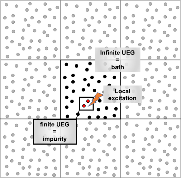
Figure 1: Schematic view of the “embedding” scheme: the two-electron finite uniform electron gas (the impurity) is embedded in the infinite uniform electron gas (the bath). The electronic excitation occurs locally, i.e., on the impurity.

One of the main driving force behind the popularity of DFT is its “universal” nature, as xc density functionals can be applied to any electronic system. Obviously, the two-electron-based density-functional approximation for ensemble defined in Eq. (54) does not have this feature as it does depend on the number of electrons constituting the finite uniform electron gas. However, one can partially cure this dependency by applying a simple “embedding” scheme (illustrated in Fig. 1) in which the two-electron finite uniform electron gas (the impurity) is embedded in the infinite uniform electron gas (the bath). The weight-dependence of the correlation functional is then carried exclusively by the impurity [i.e., the functional defined in Eq. (54)], while the remaining correlation effects are provided by the bath (i.e., the usual LDA correlation functional). Following this simple strategy, which can be further theoretically justified by the generalized adiabatic connection formalism for ensembles (GACE) originally derived by Franck and Fromager, Franck and Fromager (2014) we propose to shift the two-electron-based density-functional approximation for ensemble defined in Eq. (54) as follows:

$$\tilde{\epsilon}_{\rm c}^{\boldsymbol{w}}(n)\rightarrow{\epsilon_{\text{c}}^{{\boldsymbol{w}}}(n)}=(1-w_{1}-w_{2})\overline{\epsilon}_{\text{c}}^{(0)}(n)+w_{1}\overline{\epsilon}_{\text{c}}^{(1)}(n)+w_{2}\overline{\epsilon}_{\text{c}}^{(2)}(n),$$ (55)

where

$$\overline{\epsilon}_{\text{c}}^{(I)}(n)=\epsilon_{\text{c}}^{(I)}(n)+\epsilon_{\text{c}}^{\text{LDA}}(n)-\epsilon_{\text{c}}^{(0)}(n).$$ (56)

In the following, we will use the LDA correlation functional that has been specifically designed for 1D systems in Ref. Loos, 2013:

$$\epsilon_{\text{c}}^{\text{LDA}}(n)=a_{1}^{\text{LDA}}F\quantity[1,\frac{3}{2},a_{3}^{\text{LDA}},\frac{a_{1}^{\text{LDA}}(1-a_{3}^{\text{LDA}})}{a_{2}^{\text{LDA}}}{n}^{-1}],$$ (57)

where $F(a,b,c,x)$ is the Gauss hypergeometric function, Olver et al. (2010) and

$$a_{1}^{\text{LDA}} =-\frac{\pi^{2}}{360},$$ (58a)

$$a_{2}^{\text{LDA}} =\frac{3}{4}-\frac{\ln{2\pi}}{2},$$ (58b)

$$a_{3}^{\text{LDA}} =2.408779.$$ (58c)

Note that the strategy described in Eq. (55) is general and can be applied to real (higher-dimensional) systems. In order to make the connection with the GACE formalism Franck and Fromager (2014); Deur, Mazouin, and Fromager (2017) more explicit, one may recast Eq. (55) as

$$\begin{split}{\epsilon_{\text{c}}^{{\boldsymbol{w}}}(n)}&=\epsilon_{\text{c}}^{\text{LDA}}(n)\\ &+w_{1}\quantity[\epsilon_{\text{c}}^{(1)}(n)-\epsilon_{\text{c}}^{(0)}(n)]+w_{2}\quantity[\epsilon_{\text{c}}^{(2)}(n)-\epsilon_{\text{c}}^{(0)}(n)],\end{split}$$ (59)

or, equivalently,

$${\epsilon_{\text{c}}^{{\boldsymbol{w}}}(n)}=\epsilon_{\text{c}}^{\text{LDA}}(n)+\sum_{K>0}\int_{0}^{w_{K}}\quantity[\epsilon_{\text{c}}^{(K)}(n)-\epsilon_{\text{c}}^{(0)}(n)]d\xi_{K},$$ (60)

where the $K$th correlation excitation energy (per electron) is integrated over the ensemble weight $\xi_{K}$ at fixed (uniform) density $n$. Equation (60) nicely highlights the centrality of the LDA in the present density-functional approximation for ensembles. In particular, ${\epsilon_{\text{c}}^{(0,0)}(n)}=\epsilon_{\text{c}}^{\text{LDA}}(n)$. Consequently, in the following, we name this correlation functional “eLDA” as it is a natural extension of the LDA for ensembles. Finally, we note that, by construction,

$${\partialderivative{\epsilon_{\text{c}}^{{\boldsymbol{w}}}(n)}{w_{J}}=\epsilon_{\text{c}}^{(J)}(n)-\epsilon_{\text{c}}^{(0)}(n).}$$ (61)

IV Computational details

Having defined the eLDA functional in the previous section [see Eq. (59)], we now turn to its validation. Our testing playground for the validation of the eLDA functional is the ubiquitous “electrons in a box” model where $N$ electrons are confined in a 1D box of length $L$, a family of systems that we call $N$-boxium in the following. In particular, we investigate systems where $L$ ranges from $\pi/8$ to $8\pi$ and $2\leq N\leq 7$. These inhomogeneous systems have non-trivial electronic structure properties which can be tuned by varying the box length. For small $L$, the system is weakly correlated, while strong correlation effects dominate in the large-$L$ regime. Rogers and Loos (2017); Rogers, Ball, and Loos (2016) The one-electron density in these two regimes of correlation is represented in Fig. 2.

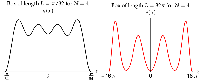
Figure 2: Ground-state one-electron density $n(x)$ of 4-boxium (i.e., $N=4$) for $L=\pi/32$ (left) and $L=32\pi$ (right). In the weak correlation regime (small box length), the one-electron density is much more delocalized and uniform than in the strong correlation regime (large box length), where a Wigner crystal starts to appear. Rogers and Loos (2017); Rogers, Ball, and Loos (2016)

We use as basis functions the (orthonormal) orbitals of the one-electron system, i.e.,

$$\chi_{\mu}(x)=\begin{cases}\sqrt{2/L}\cos(\mu\pi x/L),&\mu\text{ is odd,}\\ \sqrt{2/L}\sin(\mu\pi x/L),&\mu\text{ is even,}\end{cases}$$ (62)

with $\mu=1,\ldots,K$ and $K=30$ for all calculations. The convergence threshold $\tau=\max{\absolutevalue{\boldsymbol{F}^{{\boldsymbol{w}}}\boldsymbol{\Gamma}^{{\boldsymbol{w}}}\boldsymbol{S}-\boldsymbol{S}\boldsymbol{\Gamma}^{{\boldsymbol{w}}}\boldsymbol{F}^{{\boldsymbol{w}}}}}$ [see Eq. (36)] of the KS-DFT self-consistent calculation is set to $10^{-5}$. In order to compute the various density-functional integrals that cannot be performed in closed form, a 51-point Gauss-Legendre quadrature is employed.

In order to test the present eLDA functional we perform various sets of calculations. To get reference excitation energies for both the single and double excitations, we compute full configuration interaction (FCI) energies with the Knowles-Handy FCI program described in Ref. Knowles and Handy, 1989. For the single excitations, we also perform time-dependent LDA (TDLDA) calculations [i.e., TDDFT with the LDA functional defined in Eq. (57)]. Its Tamm-Dancoff approximation version (TDA-TDLDA) is also considered. Dreuw and Head-Gordon (2005)

Concerning the ensemble calculations, two sets of weight are tested: the zero-weight (ground-state) limit where ${\boldsymbol{w}}=(0,0)$ and the equi-triensemble (or equal-weight state-averaged) limit where ${\boldsymbol{w}}=(1/3,1/3)$. Note that a zero-weight calculation does correspond to a ground-state KS calculation with $100\%$ exact exchange and LDA correlation.

V Results and discussion

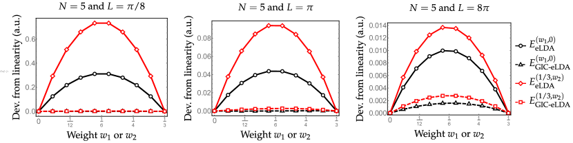
Figure 3: Deviation from linearity of the weight-dependent KS-eLDA ensemble energy $E_{\text{eLDA}}^{(w_{1},w_{2})}$ with (dashed lines) and without (solid lines) ghost-interaction correction (GIC) for 5-boxium (i.e., $N=5$) with a box of length $L=\pi/8$ (left), $L=\pi$ (center), and $L=8\pi$ (right).

First, we discuss the linearity of the computed (approximate) ensemble energies. To do so, we consider 5-boxium with box lengths of $L=\pi/8$, $L=\pi$, and $L=8\pi$, which correspond (qualitatively at least) to the weak, intermediate, and strong correlation regimes, respectively. The deviation from linearity of the three-state ensemble energy $E_{\text{}}^{(w_{1},w_{2})}$ (i.e., the deviation from the linearly-interpolated ensemble energy) is represented in Fig. 3 as a function of $w_{1}$ or $w_{2}$ while fulfilling the restrictions on the ensemble weights to ensure the GOK variational principle [i.e., $0\leq w_{2}\leq 1/3$ and $w_{2}\leq w_{1}\leq(1-w_{2})/2$]. More precisely, we follow a continuous path that connects ground-state [${\boldsymbol{w}}=(0,0)$] and equiensemble [${\boldsymbol{w}}=(1/3,1/3)$] calculations. For convenience, we use two connected paths. The first one, for which $w_{2}=0$ and $0\leq w_{1}\leq 1/3$, relies on the biensemble while the second one is defined as follows: $w_{1}=1/3$ and $0\leq w_{2}\leq 1/3$. To illustrate the magnitude of the ghost-interaction error, we report the KS-eLDA ensemble energy with and without GIC as explained above [see Eqs. (42) and (50)]. As one can see in Fig. 3, without GIC, the ensemble energy becomes less and less linear as $L$ gets larger, while the GIC reduces the curvature of the ensemble energy drastically. It is important to note that, even though the GIC removes the explicit quadratic Hx terms from the ensemble energy, a non-negligible curvature remains in the GIC-eLDA ensemble energy when the electron correlation is strong. The latter ensemble energy is computed as the weighted sum of the individual KS-eLDA energies [see Eq. (50)]. Therefore, its curvature can only originate from the weight dependence of the individual energies. Note that such a dependence does not exist in the exact theory. Here, the individual density-functional eLDA correlation energies exhibit an explicit linear and quadratic dependence on the weights, as discussed further in the next paragraph. Note also that the individual KS-eLDA energies may gain an additional (implicit) dependence on the weights through the optimization of the ensemble KS orbitals in the presence of ghost-interaction errors [see Eqs. (35) and (39)].

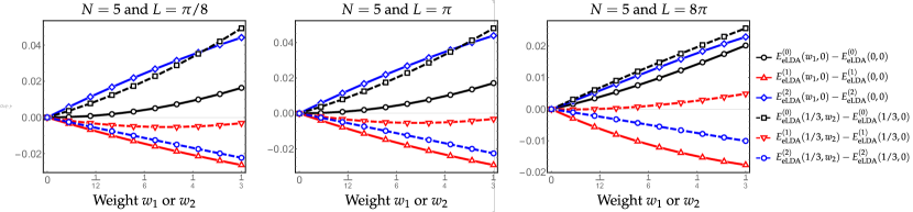
Figure 4: KS-eLDA individual energies, $E_{\text{eLDA}}^{(0)}$ (black), $E_{\text{eLDA}}^{(1)}$ (red), and $E_{\text{eLDA}}^{(2)}$ (blue), as functions of the weights $w_{1}$ (solid) and $w_{2}$ (dashed) for 5-boxium (i.e., $N=5$) with a box of length $L=\pi/8$ (left), $L=\pi$ (center), and $L=8\pi$ (right).

Figure 4 reports the behavior of the three KS-eLDA individual energies as functions of the weights. Unlike in the exact theory, we do not obtain straight horizontal lines when plotting these energies, which is in agreement with the curvature of the GIC-eLDA ensemble energy discussed previously. The variations in the ensemble weights are essentially linear or quadratic. This can be rationalized as follows. As readily seen from Eqs. (43) and (44), the individual HF-like energies do not depend explicitly on the weights, which means that the above-mentioned variations originate from the eLDA correlation functional [second and third terms on the right-hand side of Eq. (43)]. If, for analysis purposes, we consider the Taylor expansions around the uniform density regime in Eqs. (47) and (49), contributions with an explicit weight dependence still remain after summation. As both the ensemble density and the ensemble correlation energy per particle vary linearly with the weights ${\boldsymbol{w}}$ [see Eqs. (27), (28), and (41)], the latter contributions will contain both linear and quadratic terms in ${\boldsymbol{w}}$, as evidenced by Eq. (49) [see the second term on the right-hand side].
Interestingly, the individual energies do not vary in the same way depending on the state considered and the value of the weights. On one hand, we see for example that, within the biensemble (i.e., $w_{2}=0$), the energies of the ground and second excited-state increase with respect to the first-excited-state weight $w_{1}$, thus showing that, in this case, we “deteriorate” these states by optimizing the orbitals for the ensemble, rather than for each state separately. The singly excited state is, on the other hand, stabilized in the biensemble, which is reasonable as the weight associated with this state increases. For the triensemble, as $w_{2}$ increases, the energy of the ground state increases, while the energy of the first excited state remains stable with a slight increase at large $L$. The second excited state is obviously stabilized by the increase of its weight in the ensemble. These are all very sensible observations.
Let us finally stress that the (well-known) poor performance of the combined 100% HF-exchange/LDA correlation scheme in ground-state [i.e., ${\boldsymbol{w}}=(0,0)$] DFT, where the correlation energy is overestimated, is substantially improved for the ground state within the equiensemble [${\boldsymbol{w}}=(1/3,1/3)$] (see the supplementary material for further details). This is a remarkable and promising result. A similar improvement is observed for the first excited state, at least in the weak correlation regime, without deteriorating too much the second-excited-state energy.

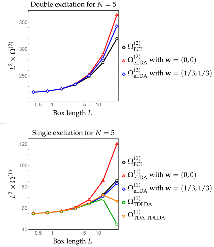
Figure 5: Excitation energies (multiplied by $L^{2}$) associated with the single excitation $\Omega_{\text{}}^{(1)}$ (bottom) and double excitation $\Omega_{\text{}}^{(2)}$ (top) of 5-boxium for various methods and box lengths $L$. Graphs for additional values of $N$ can be found as supplementary material.

Figure 5 reports the excitation energies (multiplied by $L^{2}$) for various methods and box lengths in the case of 5-boxium (i.e., $N=5$). Similar graphs are obtained for the other $N$ values and they can be found in the supplementary material alongside the numerical data associated with each method. For small $L$, the single and double excitations can be labeled as “pure”, as revealed by a thorough analysis of the FCI wavefunctions. In other words, each excitation is dominated by a sole, well-defined reference Slater determinant. However, when the box gets larger (i.e., as $L$ increases), there is a strong mixing between the different excitation degrees. In particular, the single and double excitations strongly mix, which makes their assignment as single or double excitations more disputable. Loos et al. (2019) This can be clearly evidenced by the weights of the different configurations in the FCI wave function.

As shown in Fig. 5, all methods provide accurate estimates of the excitation energies in the weak correlation regime (i.e., small $L$). When the box gets larger, they start to deviate. For the single excitation, TDLDA is extremely accurate up to $L=2\pi$, but yields more significant errors at larger $L$ by underestimating the excitation energies. TDA-TDLDA slightly corrects this trend thanks to error compensation. Concerning the eLDA functional, our results clearly evidence that the equiweight [i.e., ${\boldsymbol{w}}=(1/3,1/3)$] excitation energies are much more accurate than the ones obtained in the zero-weight limit [i.e., ${\boldsymbol{w}}=(0,0)$]. This is especially true, in the strong correlation regime, for the single excitation which is significantly improved by using equal weights. The effect on the double excitation is less pronounced. Overall, one clearly sees that, with equal weights, KS-eLDA yields accurate excitation energies for both single and double excitations. This conclusion is verified for smaller and larger numbers of electrons (see supplementary material). Except for the two-electron system where we observe cases of underestimation, eLDA usually overestimates double excitations, as evidenced by the numerical data gathered in the supplementary material.

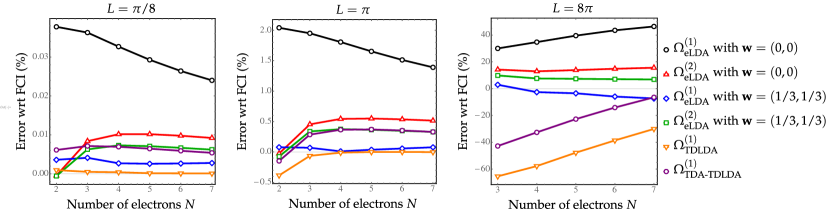
Figure 6: Error with respect to FCI in single and double excitation energies for $N$-boxium for various methods and electron numbers $N$ at $L=\pi/8$ (left), $L=\pi$ (center), and $L=8\pi$ (right).

For the same set of methods, Fig. 6 reports the error (in %) in excitation energies (as compared to FCI) as a function of $N$ for three values of $L$ ($\pi/8$, $\pi$, and $8\pi$). We draw similar conclusions as above: irrespectively of the number of electrons, the eLDA functional with equal weights is able to accurately model single and double excitations, with a very significant improvement brought by the equiensemble KS-eLDA orbitals as compared to their zero-weight (i.e., conventional ground-state) analogs. As a rule of thumb, in the weak and intermediate correlation regimes, we see that the single excitation obtained from equiensemble KS-eLDA is of the same quality as the one obtained in the linear response formalism (such as TDLDA). On the other hand, the double excitation energy only deviates from the FCI value by a few tenth of percent. Moreover, we note that, in the strong correlation regime (right graph of Fig. 6), the single excitation energy obtained at the equiensemble KS-eLDA level remains in good agreement with FCI and is much more accurate than the TDLDA and TDA-TDLDA excitation energies which can deviate by up to $60\%$. This also applies to the double excitation, the discrepancy between FCI and equiensemble KS-eLDA remaining of the order of a few percents in the strong correlation regime. These observations nicely illustrate the robustness of the GOK-DFT scheme in any correlation regime for both single and double excitations. This is definitely a very pleasing outcome, which additionally shows that, even though we have designed the eLDA functional based on a two-electron model system, the present methodology is applicable to any 1D electronic system, i.e., a system that has more than two electrons.

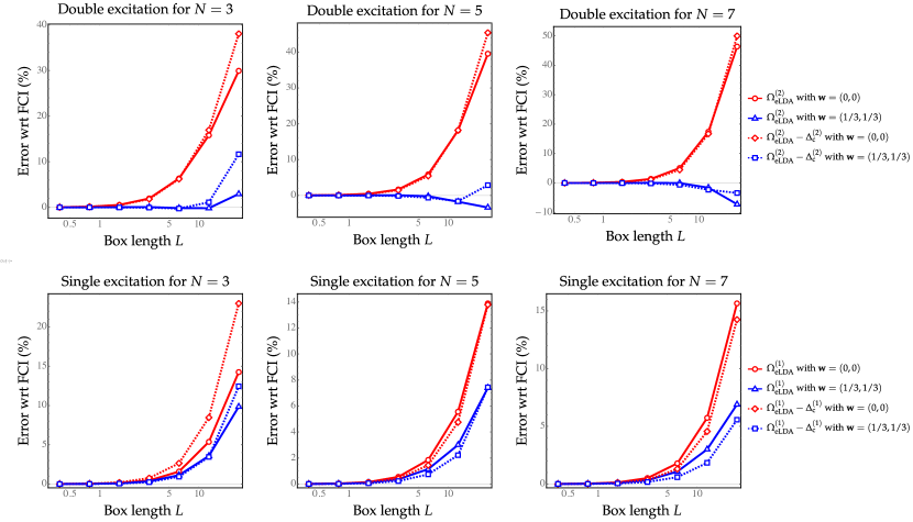
Figure 7: Error with respect to FCI (in %) associated with the single excitation $\Omega_{\text{}}^{(1)}$ (bottom) and double excitation $\Omega_{\text{}}^{(2)}$ (top) as a function of the box length $L$ for 3-boxium (left), 5-boxium (center), and 7-boxium (right) at the KS-eLDA level with and without the contribution of the ensemble correlation derivative $\Delta_{\text{c}}^{(I)}$. Zero-weight (i.e., $w_{1}=w_{2}=0$, red lines) and equiweight (i.e., $w_{1}=w_{2}=1/3$, blue lines) calculations are reported.

It is also interesting to investigate the influence of the correlation ensemble derivative contribution $\Delta_{\text{c}}^{(I)}$ to the $I$th excitation energy [see Eq. (52)]. In our case, both single ($I=1$) and double ($I=2$) excitations are considered. To do so, we have reported in Fig. 7, for $N=3$, $5$, and $7$, the error percentage (with respect to FCI) as a function of the box length $L$ on the excitation energies obtained at the KS-eLDA level with and without $\Delta_{\text{c}}^{(I)}$ [i.e., the last term in Eq. (51)]. We first stress that although for $N=3$ both single and double excitation energies are systematically improved (as the strength of electron correlation increases) when taking into account the correlation ensemble derivative, this is not always the case for larger numbers of electrons. For 3-boxium, in the zero-weight limit, the correlation ensemble derivative is significantly larger for the single excitation as compared to the double excitation; the reverse is observed in the equal-weight triensemble case. However, for 5- and 7-boxium, it hardly influences the double excitation (except when the correlation is strong), and slightly deteriorates the single excitation in the intermediate and strong correlation regimes. This non-systematic behavior in terms of the number of electrons might be a consequence of how we constructed eLDA. Indeed, as mentioned in Sec. III, the weight dependence of the eLDA functional is based on a two-electron finite uniform electron gas. Incorporating a $N$-dependence in the functional through the curvature of the Fermi hole, in the spirit of Ref. Loos, 2017, would be valuable in this respect. This is left for future work. Interestingly, for the single excitation in 3-boxium, the magnitude of the correlation ensemble derivative is substantially reduced when switching from a zero-weight to an equal-weight calculation, while giving similar excitation energies, even in the strongly correlated regime. A possible interpretation is that, at least for the single excitation, equiensemble orbitals partially remove the burden of modelling properly the correlation ensemble derivative. This conclusion does not hold for larger numbers of electrons ($N=5$ or $7$), possibly because eLDA extracts density-functional correlation ensemble derivatives from a two-electron uniform electron gas, as mentioned previously. For the double excitation, the ensemble derivative remains important, even in the equiensemble case. To summarize, the equiensemble calculation is always more accurate than a zero-weight (i.e., a conventional ground-state DFT) one, with or without including the ensemble derivative correction. Note that the second term on the right-hand side of Eq. (51), which involves the weight-dependent correlation potential and the density difference between ground and excited states, has a negligible effect on the excitation energies (results not shown).

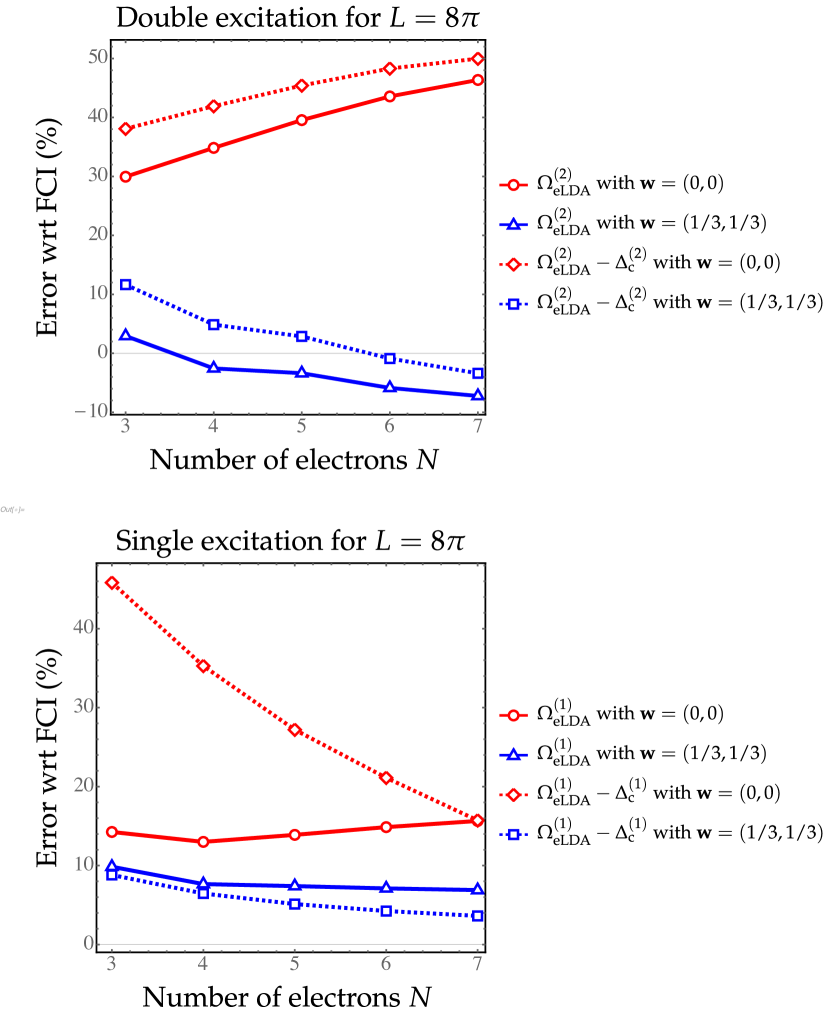
Figure 8: Error with respect to FCI in single and double excitation energies for $N$-boxium (with a box length of $L=8\pi$) as a function of the number of electrons $N$ at the KS-eLDA level with and without the contribution of the ensemble correlation derivative $\Delta_{\text{c}}^{(I)}$. Zero-weight (i.e., $w_{1}=w_{2}=0$, red lines) and equiweight (i.e., $w_{1}=w_{2}=1/3$, blue lines) calculations are reported.

Finally, in Fig. 8, we report the same quantities as a function of the electron number for a box of length $8\pi$ (i.e., in the strong correlation regime). The difference between the solid and dashed curves undoubtedly show that the correlation ensemble derivative has a rather significant impact on the double excitation (around $10\%$) with a slight tendency of worsening the excitation energies in the case of equal weights, as the number of electrons increases. It has a rather large influence (which decreases with the number of electrons) on the single excitation energies obtained in the zero-weight limit, showing once again that the usage of equal weights has the benefit of significantly reducing the magnitude of the correlation ensemble derivative.

VI Concluding remarks

A local and ensemble-weight-dependent correlation density-functional approximation (eLDA) has been constructed in the context of GOK-DFT for spin-polarized triensembles in 1D. The approach is general and can be extended to real (three-dimensional) systems Loos and Gill (2009a, b, 2010a, 2010b); Loos (2017) and larger ensembles in order to model excited states in molecules and solids. Work is currently in progress in this direction.

Unlike any standard functional, eLDA incorporates derivative discontinuities through its weight dependence. The latter originates from the finite uniform electron gas on which eLDA is (partially) based. The KS-eLDA scheme, where exact individual exchange energies are combined with the eLDA correlation functional , delivers accurate excitation energies for both single and double excitations, especially when an equiensemble is used. In the latter case, the same weights are assigned to each state belonging to the ensemble. The improvement on the excitation energies brought by the KS-eLDA scheme is particularly impressive in the strong correlation regime where usual methods, such as TDLDA, fail. We have observed that, although the correlation ensemble derivative has a non-negligible effect on the excitation energies (especially for the single excitations), its magnitude can be significantly reduced by performing equiweight calculations instead of zero-weight calculations.

Let us finally stress that the present methodology can be extended to other types of ensembles like, for example, the $N$-centered ones, Senjean and Fromager (2018, ) thus allowing for the design of a LDA-type functional for the calculation of ionization potentials, electron affinities, and fundamental gaps. Like in the present eLDA, such a functional would incorporate the infamous derivative discontinuity contribution to the fundamental gap through its explicit weight dependence. We hope to report on this in the near future.

Supplementary material

See supplementary material for the additional details about the construction of the functionals, raw data and additional graphs.

Data availability statement

The data that supports the findings of this study are available within the article [and its supplementary material].