Factorization of Antenna Efficiency of Aperture-type antenna: Beam Coupling and Two Spillovers

Abstract

Antenna efficiency is one of the most important figures-of-merit of a radio telescope for observations especially at millimeter wavelengths or shorter wavelengths, even for a multibeam radio telescope. To analyze a system with a beam waveguide, a lossless antenna consisting of two apertures in series is considered in the frame of the scalar wave approximation. We found that the antenna efficiency can be evaluated with the field distribution over the second aperture, and that the antenna efficiency is factorized into three factors: efficiencies of beam coupling, transmission spillover, and reception spillover. The factorization is applicable to general aperture-type antennas with beam waveguides, and can relate the aperture efficiency to the pupil function. We numerically confirmed our factorization with an optical simulation. This evaluation enables us to manage the aberrations and is useful in design of multibeam radio telescopes.

I Introduction

A radio telescope is a directional antenna dedicated to observing extremely weak signals which come from the universe. Single-dish radio telescopes with a single pencil beam have been developed well so far and the theory describing a single-beam radio telescope is well-established. It enables us to design a single-beam telescope with a finer beam shape, wider frequency range, and higher sensitivity. Radio astronomers and astrophysicists, however, are now eager to survey a large area of the sky, e.g. [1, 2, 3], and make a statistically significant study, e.g. [4, 5, 6]. These demands lead us to develop multibeam telescopes equipped with detector arrays with a large number of pixels.

The antenna efficiency of an aperture-type antenna [7], is one of the most important properties of a radio telescope [8], especially at millimeter wavelengths or shorter wavelengths. It is known to be related to the aperture shape and illumination (e.g [9, 10, 11, 12] ) and is decomposed into subefficiencies of spillover, polarization, illumination taper, and phase [13]. If a fundamental-mode Gaussian beam is employed for an axisymmetric telescope, the spillover efficiency and the illumination taper efficiency are a function of the illumination edge taper [14] and it is easy to calculate them by hand. The polarization and phase efficiencies are designed to be nearly unity, though degradation of these efficiencies can result from feed illumination non-uniformity in polarization and phase caused by aberrations of telescope optics.

Optimizing feed position can cancel out the tip/tilt and defocus for a telescope with a few beams. For a multibeam system with a detector array of thousands of pixels, however, it is difficult to adjust the characteristics of each feed. Moreover, the displacement of off-axis feeds from the focus normally causes aberrations [15, 16]. To manage aberration of such a system, freeform surfaces and reimaging optics can be used (e.g., [17]) and the analysis of aberration is essential in polarization and phase for higher efficiencies. The key concept is the pupil [18], because the aberration is defined there as the distortion of the wavefront. The field distribution over the pupil plane, the pupil function, holds the information of the distortion induced by the imaging system. Thus, it is desirable to relate the antenna efficiency and the pupil function to design an efficient multibeam radio telescope.

In this paper, we will unveil that the antenna efficiency can be written with the pupil function. In section II, we begin with the definition of the antenna efficiency [7] to consider a dual-reflector antenna, and derive an expression of the antenna efficiency of an obliquely incident case. The intrinsic relationship between the antenna efficiency and the beam coupling efficiency [19] is shown. In section III, the consideration of the same dual-reflector system as a receiving one leads us to the efficiency evaluation at the second aperture. It turns out that the antenna efficiency can be written as the product of the beam coupling efficiency, the spillover efficiency of the feed beam, and the spillover efficiency of the incident beam. We verify the factorization with numerical simulation in Section IV, which is followed by some discussion on the new factor, its relation to the pupils, and the application of the factorization to antenna design in Section V.

II Antenna Efficiency of Antenna with two apertures in series

Single-dish radio telescopes typically have a large reflector to achieve high directivity and a beam waveguide to couple the incident radiation to the feed. Most radio telescopes employ a dual-reflector antenna such as Cassegrain, Gregorian, and Dragone telescope [20, 21], which is sometimes followed by an additional optical system. Thus, we focus on the dual-reflector antenna. If a telescope is composed of more than three mirrors, the discussion below can be applied easily.

Each reflector can be regarded as a combination of an equivalent aperture and lens, and the dual-reflector system can be regarded as an antenna with two apertures in series (Fig. 1). To be precise, an equivalent aperture can be specified for each mirror, which is included in the aperture plane perpendicular to the telescope axis. The equivalent apertures of the primary and secondary mirrors are labeled as $A_{1}$ and $A_{2}$, respectively, and their corresponding aperture planes are $P_{1}$ and $P_{2}$, respectively. The equivalent lens of a mirror represents the phase modification by the mirror. We assume that the components are passive, linear, and lossless, and that the reflectors are much larger than the operation wavelength and work as an ideal one-way beam waveguide. We also assume that the beam of the antenna in transmitting mode comes only from the antenna aperture $A_{1}$; this assumption is not essential but makes the derivation simple (See the last paragraph of this section). We do not consider aperture blocking here; the effect of blockage should be taken into account separately as the usual manner (e.g. [10]). A perfect polarization match is assumed for simplicity.

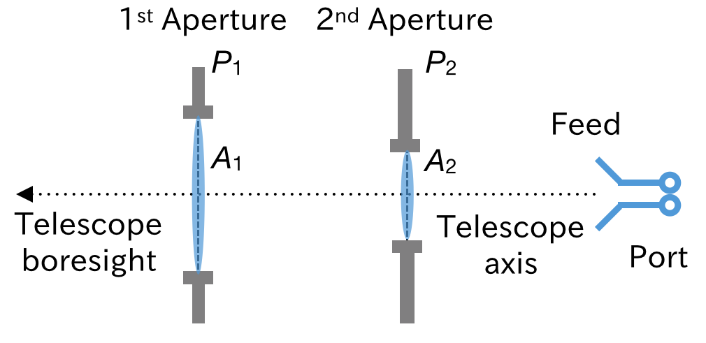
Figure 1: Antenna with two apertures in series. When the feed is on the telescope axis, the feed and its beam are called ‘on-axis’. Otherwise they are called ‘off-axis’.

The system works as a transmitting antenna when the antenna is equipped with a transmitter at its port as shown in Fig. 2 (a). We first summarize some antenna properties in the IEEE standard [7]. The antenna efficiency of this antenna is

$$\eta_{\mathrm{ant}}:=A_{\mathrm{eff}}/|A_{1}|,$$ (1)

where $A_{\mathrm{eff}}$ is the effective aperture area of the antenna and $|A_{1}|$ is the area of $A_{1}$. The effective aperture area satisfies the fundamental relation of a reciprocal antenna operating at wavelength $\lambda$,

$$\eta_{\mathrm{rad}}D_{\mathrm{pk}}=\frac{4\pi}{\lambda^{2}}A_{\mathrm{eff}},$$ (2)

where $\eta_{\mathrm{rad}}$ is the radiation efficiency and $D_{\mathrm{pk}}$ is the peak directivity. The standard directivity of the system is

$$D_{\mathrm{std}}=\frac{4\pi}{\lambda^{2}}|A_{1}|.$$ (3)

Dividing (2) by (3) gives the relation [22]:

$$\eta_{\mathrm{ant}}=\eta_{\mathrm{rad}}\eta_{\mathrm{ap}},$$ (4)

where

$$\eta_{\mathrm{ap}}:=D_{\mathrm{pk}}/D_{\mathrm{std}}$$ (5)

is the aperture illumination efficiency of this antenna.

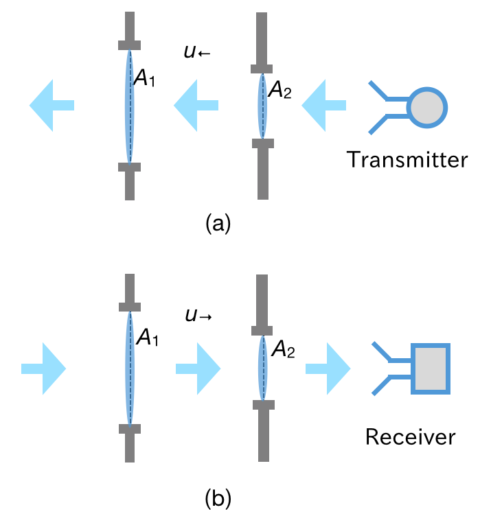
Figure 2: Antenna with two apertures in operation. (a) transmission. (b) reception.

The directivity can be written with the field distribution on $A_{1}$ explicitly. For an on-axis feed, whose electrical boresight is perpendicular to $A_{1}$, the expression is as follows [23],

$$D_{\mathrm{pk}}=\frac{4\pi}{\lambda^{2}}\frac{\left|\int_{A_{1}}u_{\leftarrow}(p)\mathrm{d}^{2}p\right|^{2}}{\int_{A_{1}}|u_{\leftarrow}(p)|^{2}\mathrm{d}^{2}p},$$ (6)

where $u_{\leftarrow}(p)$ is the complex electric field at position $p$ excited by the transmitting antenna with the scalar wave approximation. Thus, the aperture illumination efficiency (5) for the on-axis feed is written as

$$\eta_{\mathrm{ap}}=\frac{1}{|A_{1}|}\frac{\left|\int_{A_{1}}u_{\leftarrow}(p)\mathrm{d}^{2}p\right|^{2}}{\int_{A_{1}}|u_{\leftarrow}(p)|^{2}\mathrm{d}^{2}p}.$$ (7)

The expression (7) relates to the coupling between the beam from the feed and the incident plane wave [19]. Let $u_{\rightarrow}$ be the complex electric field excited by a uniform plane wave incoming from the electrical boresight. The beam coupling efficiency between $u_{\rightarrow}$ and $u_{\leftarrow}$ at $A_{1}$ is defined as

$$\eta_{\mathrm{bcp},1}:=\frac{\left|\int_{A_{1}}u_{\rightarrow}(p)u_{\leftarrow}(p)\mathrm{d}^{2}p\right|^{2}}{\int_{A_{1}}|u_{\rightarrow}(p)|^{2}\mathrm{d}^{2}p\cdot\int_{A_{1}}|u_{\leftarrow}(p)|^{2}\mathrm{d}^{2}p}.$$ (8)

The last subscript of $\eta_{\mathrm{bcp},1}$ denotes that this efficiency is defined and calculated at $A_{1}$. When the direction of $u_{\rightarrow}$ is perpendicular to $A_{1}$, the right-hand side of (8) reduces to (7) because $u_{\rightarrow}(p)$ is a constant over $A_{1}$. The beam coupling efficiency introduced here is an equivalent in scalar wave to the coupling efficiency between the incident beam and the feed pattern in [24]. In general, coupling efficiency of vector wave can be factorized into three factors: polarization ($\eta_{\mathrm{pol}}$), amplitude, and phase [19]. Here we assumed $\eta_{\mathrm{pol}}=1$ so that we can use scalar wave description. The amplitude and phase efficiency can be written as

$$\eta_{\mathrm{ill}} :=\frac{\left(\int_{A_{1}}|u_{\rightarrow}(p)||u_{\leftarrow}(p)|\mathrm{d}^{2}p\right)^{2}}{\int_{A_{1}}|u_{\rightarrow}(p)|^{2}\mathrm{d}^{2}p\cdot\int_{A_{1}}|u_{\leftarrow}(p)|^{2}\mathrm{d}^{2}p},$$ (9)

$$\eta_{\mathrm{\phi}} :=\frac{\left|\int_{A_{1}}u_{\rightarrow}(p)u_{\leftarrow}(p)\mathrm{d}^{2}p\right|^{2}}{\left(\int_{A_{1}}|u_{\rightarrow}(p)||u_{\leftarrow}(p)|\mathrm{d}^{2}p\right)^{2}},$$ (10)

which satisfies $\eta_{\mathrm{bcp},1}=\eta_{\mathrm{pol}}\eta_{\mathrm{ill}}\eta_{\mathrm{\phi}}$. These subefficiencies correspond to those in [13].

Since we need to deal with both on-axis and off-axis feeds of a multibeam telescope, we will consider the case where the electrical boresight of a feed is not necessarily perpendicular to $A_{1}$. We take the equivalent aperture perpendicular to the electrical boresight, $A_{1}^{\prime}$, so that the directivity can be calculated with the expression based on (6) by replacing $A_{1}$ with $A_{1}^{\prime}$. The standard directivity and aperture illumination efficiency with respect to $A_{1}^{\prime}$ are $D_{\mathrm{std}}^{\prime}=4\pi|A_{1}^{\prime}|/\lambda^{2}$ and

$$\eta_{\mathrm{ap}}^{\prime}:=\frac{D_{\mathrm{pk}}}{D_{\mathrm{std}}^{\prime}}=\frac{1}{|A_{1}^{\prime}|}\frac{\left|\int_{A_{1}^{\prime}}u_{\leftarrow}(p^{\prime})\mathrm{d}^{2}p^{\prime}\right|^{2}}{\int_{A_{1}^{\prime}}|u_{\leftarrow}(p^{\prime})|^{2}\mathrm{d}^{2}p^{\prime}},$$ (11)

respectively. These quantities on $A_{1}$ and $A_{1}^{\prime}$ are related by the following equations:

$$D_{\mathrm{std}}=D_{\mathrm{std}}^{\prime}/\cos\theta\quad\text{and}\quad\eta_{\mathrm{ap}}=\eta_{\mathrm{ap}}^{\prime}\cos\theta,$$ (12)

where $\theta$ is the angle between the electrical boresight and the reference boresight, since $|A_{1}^{\prime}|=|A_{1}|\cos\theta$. The aperture illumination efficiency on $A_{1}^{\prime}$ equals the beam coupling efficiency between $u_{\rightarrow}$ and $u_{\leftarrow}$ at $A_{1}^{\prime}$,

$$\eta_{\mathrm{bcp},1^{\prime}}:=\frac{\left|\int_{A_{1}^{\prime}}u_{\rightarrow}(p^{\prime})u_{\leftarrow}(p^{\prime})\mathrm{d}^{2}p^{\prime}\right|^{2}}{\int_{A_{1}^{\prime}}|u_{\rightarrow}(p^{\prime})|^{2}\mathrm{d}^{2}p^{\prime}\cdot\int_{A_{1}^{\prime}}|u_{\leftarrow}(p^{\prime})|^{2}\mathrm{d}^{2}p^{\prime}}.$$ (13)

The last subscript of $\eta_{\mathrm{bcp},1^{\prime}}$ denotes that this efficiency is defined and calculated at $A_{1}^{\prime}$. The value of $\eta_{\mathrm{bcp},1^{\prime}}$ can be approximated by $\eta_{\mathrm{bcp},1}$ when $|\theta|\ll 1$ because the correspondence between position $p$ in $A_{1}$ and $p^{\prime}$ in $A_{1}^{\prime}$ gives $\cos\theta\mathrm{d}^{2}p=\mathrm{d}^{2}p^{\prime}$ and

$$\begin{split}|u_{\rightarrow}(p)|^{2}&=|u_{\rightarrow}(p^{\prime})|^{2},\\ |u_{\leftarrow}(p)|^{2}&=|u_{\leftarrow}(p^{\prime})|^{2},\\ u_{\rightarrow}(p)u_{\leftarrow}(p)&=u_{\rightarrow}(p^{\prime})u_{\leftarrow}(p^{\prime}).\end{split}$$ (14)

These equations come from the fact that the position dependence of $|u_{\rightarrow}|$ and $|u_{\leftarrow}|$ are weak and that $u_{\rightarrow}$ and $u_{\leftarrow}$ have almost the same wavefront shape propagating in directions opposite to each other. Under this approximation the equation $\eta_{\mathrm{bcp},1}=\eta_{\mathrm{bcp},1^{\prime}}$ can be obtained from (8) and (13). Then the aperture illumination efficiency on $A_{1}$ can be expressed in terms of the field distribution over $A_{1}$,

$$\eta_{\mathrm{ap}}=\eta_{\mathrm{bcp},1}\cos\theta.$$ (15)

That is, the aperture illumination efficiency is the product of the beam coupling efficiency at the first aperture and the inclination factor $\cos\theta$. Further detailed analysis for inclined beams can be found in [25].

The power radiated by the feed is spilled over at the second and first apertures. We call this spillover ‘transmission spillover’ to distinguish it from another kind of spillover described in §III. The transmission spillover efficiencies at these apertures are given by

$$\eta_{\mathrm{sp},{2}\leftarrow{\mathrm{tx}}} :=\frac{\int_{A_{\mathrm{2}}^{\prime}}|u_{\leftarrow}(p^{\prime})|^{2}\mathrm{d}^{2}p^{\prime}}{\int_{P_{\mathrm{2}}^{\prime}}|u_{\leftarrow}(p^{\prime})|^{2}\mathrm{d}^{2}p^{\prime}}=\frac{\int_{A_{\mathrm{2}}}|u_{\leftarrow}(p)|^{2}\mathrm{d}^{2}p}{\int_{P_{\mathrm{2}}}|u_{\leftarrow}(p)|^{2}\mathrm{d}^{2}p},$$ (16)

$$\eta_{\mathrm{sp},{1}\leftarrow{2}} :=\frac{\int_{A_{1}^{\prime}}|u_{\leftarrow}(p^{\prime})|^{2}\mathrm{d}^{2}p^{\prime}}{\int_{P_{1}^{\prime}}|u_{\leftarrow}(p^{\prime})|^{2}\mathrm{d}^{2}p^{\prime}}=\frac{\int_{A_{\mathrm{1}}}|u_{\leftarrow}(p)|^{2}\mathrm{d}^{2}p}{\int_{P_{\mathrm{1}}}|u_{\leftarrow}(p)|^{2}\mathrm{d}^{2}p},$$ (17)

respectively, where $A_{2}^{\prime}$ is the equivalent aperture of the secondary mirror perpendicular to the feed’s beam axis corresponding to the electrical boresight. The middle expression of these equations represents the exact power ratio while the right-hand side follows under the same approximation as in (14). In other words, the beam inclination does not change the spillover efficiencies [25]. The total transmission spillover efficiency, which includes spillover at both apertures, can be written as

$$\eta_{\mathrm{sp}}=\eta_{\mathrm{sp},{1}\leftarrow{2}}\eta_{\mathrm{sp},{2}\leftarrow{\mathrm{tx}}}=\frac{\int_{A_{1}^{\prime}}|u_{\leftarrow}(p^{\prime})|^{2}\mathrm{d}^{2}p^{\prime}}{\int_{P_{2}^{\prime}}|u_{\leftarrow}(p^{\prime})|^{2}\mathrm{d}^{2}p^{\prime}}.$$ (18)

Here we used the conservation of the beam total power, $\int_{P_{1}^{\prime}}|u_{\leftarrow}(p^{\prime})|^{2}\mathrm{d}^{2}p^{\prime}=\int_{A_{2}^{\prime}}|u_{\leftarrow}(p^{\prime})|^{2}\mathrm{d}^{2}p^{\prime}$. Since the power reaching $A_{1}$ equals to the power radiated from the antenna, the radiation efficiency of the antenna equals the total transmission spillover efficiency, $\eta_{\mathrm{rad}}=\eta_{\mathrm{sp}}$. Thus, using (4), the antenna efficiency of this system is expressed as

$$\eta_{\mathrm{ant}}=\eta_{\mathrm{sp},{1}\leftarrow{2}}\eta_{\mathrm{sp},{2}\leftarrow{\mathrm{tx}}}\eta_{\mathrm{bcp},1}\cos\theta.$$ (19)

Note that the expression (6), (7), and equation $\eta_{\mathrm{rad}}=\eta_{\mathrm{sp}}$ are based on the assumption on beam and antenna aperture. However, the factorization (19) is valid for dual-reflector antennas because the antenna efficiency does not depend on the destination of radiation spilled over from the antenna aperture, emitted to the sky or terminated in the telescope, unless there is no far-sidelobe which points to the antenna boresight.

III Reception Spillover

When the antenna is equipped with a receiver at its port, the system works as a receiving antenna, as shown in Fig. 2 (b). The power of the uniform plane wave entering the system is defined by the first aperture. The wave diffracted by $A_{1}$ propagates to $P_{2}$ and a portion of its power passes through $A_{2}$. The rest of the power is spilled out and does not pass through $A_{2}$; this power loss can be regarded as a spillover of the radiation entering the system and we call it ‘reception spillover’. We can define an efficiency of the reception spillover at the second aperture as

$$\eta_{\mathrm{sp},{1}\rightarrow{2}}:=\eta_{\mathrm{sp},{1^{\prime}}\rightarrow{2}}\cdot\eta_{\mathrm{sp},{1}\rightarrow{1^{\prime}}}=\frac{\int_{A_{2}^{\prime}}|u_{\rightarrow}(p^{\prime})|^{2}\mathrm{d}^{2}p^{\prime}}{\int_{A_{1}}|u_{\rightarrow}(p)|^{2}\mathrm{d}^{2}p},$$ (20)

where

$$\eta_{\mathrm{sp},{1^{\prime}}\rightarrow{2}} :=\frac{\int_{A_{2}^{\prime}}|u_{\rightarrow}(p^{\prime})|^{2}\mathrm{d}^{2}p^{\prime}}{\int_{P_{2}^{\prime}}|u_{\rightarrow}(p^{\prime})|^{2}\mathrm{d}^{2}p^{\prime}}=\frac{\int_{A_{2}}|u_{\rightarrow}(p)|^{2}\mathrm{d}^{2}p}{\int_{P_{2}}|u_{\rightarrow}(p)|^{2}\mathrm{d}^{2}p},$$ (21)

$$\eta_{\mathrm{sp},{1}\rightarrow{1^{\prime}}} :=\frac{\int_{A_{1}^{\prime}}|u_{\rightarrow}(p^{\prime})|^{2}\mathrm{d}^{2}p^{\prime}}{\int_{A_{1}}|u_{\rightarrow}(p)|^{2}\mathrm{d}^{2}p}=\frac{|A_{1}^{\prime}|}{|A_{1}|}=\cos\theta.$$ (22)

The first factor $\eta_{\mathrm{sp},{1^{\prime}}\rightarrow{2}}$ is the ratio of the power passing through $A_{2}$ to the power reached to $P_{2}$, similar to (16) and (17). The second factor $\eta_{\mathrm{sp},{1}\rightarrow{1^{\prime}}}$ is the ratio of the power passing through the first aperture for the off-axis beam to that for the on-axis beam and can be regarded as the efficiency of reception spillover at $A_{1}^{\prime}$ with respect to $A_{1}$. To obtain the right-hand side of (20), the conservation of the beam total power $\int_{P_{2}^{\prime}}|u_{\rightarrow}(p^{\prime})|^{2}\mathrm{d}^{2}p^{\prime}=\int_{A_{1}^{\prime}}|u_{\rightarrow}(p^{\prime})|^{2}\mathrm{d}^{2}p^{\prime}$ is used.

We can define the beam coupling efficiency between $u_{\rightarrow}$ and $u_{\leftarrow}$ at the second aperture similar to (8) and (13),

$$\eta_{\mathrm{bcp},2} :=\frac{\left|\int_{A_{2}}u_{\rightarrow}(p)u_{\leftarrow}(p)\mathrm{d}^{2}p\right|^{2}}{\int_{A_{2}}|u_{\rightarrow}(p)|^{2}\mathrm{d}^{2}p\cdot\int_{A_{2}}|u_{\leftarrow}(p)|^{2}\mathrm{d}^{2}p}$$ (23)

$$\eta_{\mathrm{bcp},2^{\prime}} :=\frac{\left|\int_{A_{2}^{\prime}}u_{\rightarrow}(p^{\prime})u_{\leftarrow}(p^{\prime})\mathrm{d}^{2}p^{\prime}\right|^{2}}{\int_{A_{2}^{\prime}}|u_{\rightarrow}(p^{\prime})|^{2}\mathrm{d}^{2}p^{\prime}\cdot\int_{A_{2}^{\prime}}|u_{\leftarrow}(p^{\prime})|^{2}\mathrm{d}^{2}p^{\prime}},$$ (24)

respectively. Note that the fields $u_{\rightarrow}$ and $u_{\leftarrow}$ are not necessarily a plane wave. With the same argument done for $\eta_{\mathrm{bcp},1}$ and $\eta_{\mathrm{bcp},1^{\prime}}$ in §II, we can obtain $\eta_{\mathrm{bcp},2}=\eta_{\mathrm{bcp},2^{\prime}}$. The numerators of (13) and (24) are equal as a result of the beam coupling theorem applied to $A_{1}^{\prime}$ and $A_{2}^{\prime}$ (See Appendix),

$$\int_{A_{1}^{\prime}}u_{\rightarrow}(p^{\prime})u_{\leftarrow}(p^{\prime})\mathrm{d}^{2}p^{\prime}=\int_{A_{2}^{\prime}}u_{\rightarrow}(p^{\prime})u_{\leftarrow}(p^{\prime})\mathrm{d}^{2}p^{\prime}.$$ (25)

Then, we can obtain the following identity from (13), (17), (21), (24), (25), and the beam total power conservation,

$$\eta_{\mathrm{bcp},1}\cdot\eta_{\mathrm{sp},{1}\leftarrow{2}}=\eta_{\mathrm{sp},{1^{\prime}}\rightarrow{2}}\cdot\eta_{\mathrm{bcp},2}.$$ (26)

Now we can factorize the antenna efficiency with the reception spillover efficiency, by substituting (26) into (19): $\eta_{\mathrm{ant}}=\eta_{\mathrm{sp},{1^{\prime}}\rightarrow{2}}\cdot\eta_{\mathrm{bcp},2}\cdot\eta_{\mathrm{sp},{2}\leftarrow{\mathrm{tx}}}\cos\theta$. The inclination factor $\cos\theta$ can be regarded as the reception spillover efficiency $\eta_{\mathrm{sp},{1}\rightarrow{1^{\prime}}}$ and the following expression is obtained:

$$\eta_{\mathrm{ant}}=\eta_{\mathrm{sp},{1}\rightarrow{2}}\cdot\eta_{\mathrm{bcp},2}\cdot\eta_{\mathrm{sp},{2}\leftarrow{\mathrm{tx}}}.$$ (27)

That is, the antenna efficiency is the product of three efficiencies of reception spillover, beam coupling, and transmission spillover evaluated at the second aperture.

In addition, the factorization at the first aperture (19) can be written in the same form,

$$\eta_{\mathrm{ant}}=\eta_{\mathrm{sp},{1}\rightarrow{1^{\prime}}}\cdot\eta_{\mathrm{bcp},1}\cdot\eta_{\mathrm{sp}}.$$ (28)

IV Verification

We verify our factorization (27) and (28) numerically which allow evaluation of the antenna efficiency with a beam coupling efficiency, with simple telescope models as a demonstration. We calculate the efficiencies using the field distribution on mirrors based on physical optics, and compare them with the efficiencies obtained directly from the definition (1) and (5). The operation frequency of the telescope models was set to 300 GHz.

IV-A Example: Gregorian telescope models

We prepared three models of the axisymmetric classical Gregorian telescope: 1) telescope with a single beam, 2) telescope whose pupil is located at the primary mirror, and 3) telescope whose pupil is located at the secondary mirror. The diameters of the primary mirrors were set to 300 mm to keep the same standard directivity (59.491 dBi). Other common geometrical parameters are shown in Table I. This design can be described with parameters of [26]; $F$, $L_{\mathrm{m}}$, $L_{\mathrm{s}}$, $a$, $f$ are 400, 100, 400, 250, and 150 mm, respectively. The difference among the models lies in the secondary mirror size, which results in the different sizes of the pupils, as shown in Table II. The secondary mirror sizes were determined with ray-tracing to transmit the rays reflected at the primary for Model 1 and to transmit the rays through the pupil to provide a 1-degree field-of-view for Models 2 and 3. Figure 3 shows Model 2 as an example. The feeds were put on the system axis for all models, and a 1-degree off-axis position for Models 2 and 3. Thus, we have 5 cases to consider (cf. Table III). The beam waists were placed so that the radius of curvature of the beam wavefront at the secondary mirror become identical with the distance between the secondary mirror and the focus.

To determine the antenna properties and the field distribution on the mirrors for the five cases, we used the physical optics (PO) simulation software GRASP [27]. The telescope for each case in the PO simulation was operated in both transmitting and receiving modes, where the blocking by the secondary mirror and the feed was not taken into account. A uniform plane wave entered the telescope from the electrical boresight for the receiving mode while a fundamental-mode Gaussian beam was emitted by the feed for the transmitting mode. We set the Gaussian beam size for all cases so that the edge taper of the secondary mirror (Model 1) or the exit pupil (Models 2 and 3), $T_{\mathrm{e}}$, is 13 dB.

TABLE I: Common parameters of telescope models

	Radius of	Conic	Distance to
	curvature	constant	next surface
	[mm]	–	[mm]
Primary	$-800$	$-1$	$-500$
Secondary	$160$	$-0.36$	$400$
Focal plane	$200$	0	–

TABLE II: Diameters of elements in Gregorian telescope models

	Primary	Secondary	Entrance	Exit
	Mirror	Mirror	Pupil	Pupil
Model	[mm]	[mm]	[mm]	[mm]
1) Single beam	300	74.4	-	-
2) Pupil at primary	300	92.0	300	57.3
3) Pupil at secondary	300	57.5	230.5	57.5

Figure 3: The optical design for the Gregorian telescope whose pupil is located at the primary mirror (Model 2). The vertical dashed-dotted line at $z\approx 200$ mm represents the exit pupil of this system.

The antenna properties determined with the PO simulation in the transmitting mode are shown in Table III. The transmission spillover efficiencies are derived from the power radiated by the feed and the power entering the corresponding mirror. The peak directivity and the effective aperture area are derived from the peak gain. The fiducial aperture illumination efficiency $\eta_{\mathrm{ap}}$ and the fiducial antenna efficiency $\eta_{\mathrm{ant}}$ are given by (5) and (1), respectively. We can confirm that the values in Table III satisfy (4). The $\eta_{\mathrm{sp},{1}\leftarrow{2}}$ values of Model 3 are almost unity since the feed beam truncated by the secondary mirror is fully covered by the primary mirror and the loss is due to higher-order diffraction. The conventional formula for the spillover efficiency and the illumination taper efficiency [28, 14] gives

$$\eta_{\mathrm{sp}} =1-e^{-2\alpha}\approx 0.94988,$$ (29)

$$\eta_{\mathrm{ill}} =\frac{2\left(1-e^{-\alpha}\right)^{2}}{\alpha\left(1-e^{-2\alpha}\right)}\approx 0.84742,$$ (30)

respectively, where $\alpha=(T_{\mathrm{e}}\ln 10)/20\approx 1.4967$ is the beam truncation parameter. The $\eta_{\mathrm{sp}}$ values in Table III are close to the value in (29). The $\eta_{\mathrm{ill}}$ values of Models 1 and 2 are close to the value in (30) while those of Model 3 are significantly smaller than it. This degradation indicates that only a part of the primary mirror is illuminated by the feed beam in Model 3 as expected. The values in Table III are a reference for the discussion in the next section.

TABLE III: Antenna properties of model telescopes

	$\eta_{\mathrm{sp},{2}\leftarrow{\mathrm{tx}}}$	$\eta_{\mathrm{sp},{1}\leftarrow{2}}$	$\eta_{\mathrm{sp}}$	$D_{\mathrm{pk}}$	$\eta_{\mathrm{ap}}$	$A_{\mathrm{eff}}$	$\eta_{\mathrm{ant}}$
Case				[dBi]		[mm2]
1) Single beam	0.9529	0.9871	0.9406	58.294	0.8069	53647	0.7590
2-1) Pupil at primary, on axis	0.9876	0.9571	0.9452	58.604	0.8624	57620	0.8152
2-2) Pupil at primary, off axis	0.9801	0.9649	0.9456	58.490	0.8398	56123	0.7941
3-1) Pupil at secondary, on axis	0.9517	0.9955	0.9474	56.369	0.5143	34444	0.4873
3-2) Pupil at secondary, off axis	0.9513	0.9921	0.9438	56.265	0.5041	33625	0.4758

IV-B Factors with beam coupling efficiency

We calculated the antenna efficiency for each case, using the beam coupling efficiencies (8) and (23) from the simulated electric field distribution on each mirror, where for the integrand in the numerator we used the inner product of the electric field vectors. Including them, all the factors in the factorization of the antenna efficiency, (27) and (28), are listed in Table IV. The antenna efficiencies evaluated at $A_{1}$ and $A_{2}$ are denoted by $\eta_{\mathrm{ant};1}$ and $\eta_{\mathrm{ant};2}$, respectively. The transmission spillover efficiencies are adopted from Table III. The reception spillover efficiencies are derived from the power accepted by the primary mirror at normal incidence and the power reflected by the corresponding mirror, which are obtained with the PO simulation in the receiving mode. The antenna efficiencies obtained from the beam coupling efficiency agree well with the fiducial value for all cases (better than 0.1%).

TABLE IV: Efficiencies of reception spillover, beam coupling, and transmission spillover

	Primary mirror				Secondary mirror
Case	$\eta_{\mathrm{ant};1}$	$\eta_{\mathrm{sp},{1}\rightarrow{1^{\prime}}}$	$\eta_{\mathrm{bcp},1}$	$\eta_{\mathrm{sp}}$	$\eta_{\mathrm{ant};2}$	$\eta_{\mathrm{sp},{1}\rightarrow{2}}$	$\eta_{\mathrm{bcp},2}$	$\eta_{\mathrm{sp},{2}\leftarrow{\mathrm{tx}}}$
1	0.7590	1.0000	0.8069	0.9406	0.7581	0.9313	0.8542	0.9529
2-1	0.8152	1.0000	0.8624	0.9452	0.8156	0.9793	0.8434	0.9876
2-2	0.7940	0.9998	0.8398	0.9456	0.7938	0.9695	0.8354	0.9801
3-1	0.4874	1.0000	0.5144	0.9474	0.4871	0.6410	0.7985	0.9517
3-2	0.4754	0.9998	0.5038	0.9438	0.4756	0.6050	0.8263	0.9513

The factors in Table IV allow us to evaluate some effects on the antenna efficiency. The reception spillover efficiency at the primary mirror $\eta_{\mathrm{sp},{1}\rightarrow{1^{\prime}}}$ are unity or $\cos 1^{\circ}$. Almost all the beam coupling efficiency $\eta_{\mathrm{bcp},1}$ and $\eta_{\mathrm{bcp},2}$ are close to the illumination taper efficiency given by (30). Exceptionally, $\eta_{\mathrm{bcp},1}$ of Model 3 have completely different values from $\eta_{\mathrm{ill}}$ in (30) since they include the effect of partial illumination of the antenna aperture. The reception spillover efficiencies at the secondary mirror $\eta_{\mathrm{sp},{1}\rightarrow{2}}$ of Models 1 and 2 decrease by several percents because of diffraction though geometrical optics predicts unity. In contrast, the $\eta_{\mathrm{sp},{1}\rightarrow{2}}$ values of Model 3 are significantly lower because some of the energy entering $A_{1}$ is spilled out at $A_{2}$ which truncates the entering beam as the stop. These values confirm that the partial illumination of the antenna aperture and the reception spillover is closely related. In short, $\eta_{\mathrm{bcp},2}$ represents the degree of matching between the incident beam and the feed beam, and $\eta_{\mathrm{sp},{1}\rightarrow{2}}$ represents the degree of the reception spillover, while $\eta_{\mathrm{bcp},1}$ includes both effects because $A_{1}$ is not a pupil in Model 3.

V Discussion

V-A Reception spillover efficiency

We found that the antenna efficiency of the aperture type can be factorized at an aperture into three factors: the beam coupling efficiency, the transmission spillover efficiency, and the reception spillover efficiency. The reception spillover has not been pointed out explicitly in previous works as far as we know. This is probably because the reception spillover efficiency of a single-beam radio telescope can reach almost unity by setting the size of the reflectors to fit the sole beam, and can be negligible as a factor of the antenna efficiency. Further, one can design a multibeam radio telescope free from reception spillover except for the beam inclination effect when it has only one aperture, or more generally when its entrance pupil is located at its first optical element. Otherwise, the reception spillover should be taken into account.

The reception spillover at the entrance pupil can be interpreted geometrically. Figure 4 shows a schematic view of a multibeam Cassegrain telescope. Beam edges are drawn as straight lines according to geometrical optics. In this example, the secondary mirror as a stop defines the edge of every beam from the sky to the focal plane. The exit pupil is the secondary mirror itself, and the entrance pupil is its image made by the primary mirror. Thus, there exist the rays that reflect at the primary mirror but do not hit the secondary mirror. The reception spillover efficiency at the entrance pupil indicates how much the energy entering the system can pass through all the optical components in the system.

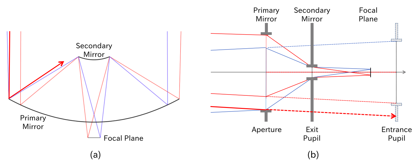
Figure 4: Multibeam Cassegrain telescope whose secondary mirror works as a stop: (a) schematic view and (b) beam propagation. Rays at the beam edge are shown (thin lines). A ray spilled by the secondary mirror (entrance pupil) is also shown (arrows with thick lines).

V-B Application to multibeam telescope design

The beam coupling efficiency and the transmission and reception spillover efficiencies can be utilized in design of multibeam radio telescopes. Though the beam coupling efficiency can be calculated at any aperture in the system, the best position for this purpose is at a pupil. This is because all the beams illuminate the same region in a pupil plane and a pupil is fully illuminated by definition. In addition, the amplitude distributions of the beam field on the pupils are similar to each other [29], which means that the powers passing through the pupils are equal. Thus, as a result of the beam coupling theorem, all the beam coupling efficiencies on the pupils become the same, which we write as $\eta_{\mathrm{bcp},\mathrm{pup}}$. We can choose one of the pupils to calculate $\eta_{\mathrm{bcp},\mathrm{pup}}$. The reception spillover efficiency from the first aperture to a pupil and the transmission spillover efficiency from the feed to a pupil are also invariant on the pupils. The former can be calculated most easily at the entrance pupil and the latter at the exit pupil, written as $\eta_{\mathrm{sp},\mathrm{ent}}$ and $\eta_{\mathrm{sp},\mathrm{ext}}$, respectively. Now we can write the factorization of the antenna efficiency at the pupils as follows:

$$\eta_{\mathrm{ant}}=\eta_{\mathrm{sp},\mathrm{ent}}\cdot\eta_{\mathrm{bcp},\mathrm{pup}}\cdot\eta_{\mathrm{sp},\mathrm{ext}}.$$ (31)

This factorization separates the contribution of beam coupling from two spillovers. This separation is useful because the effect of aberrations appear mainly in the beam coupling, especially in polarization and phase.

The three factors in (31) can be obtained with PO simulations in the transmitting and receiving modes as shown in Sect. IV. Here let us consider a simple way to calculate them for a system with circular apertures with some approximation. When a telescope has no aberrations and a fundamental-mode Gaussian beam is employed as a feed, $\eta_{\mathrm{bcp},\mathrm{pup}}$ and $\eta_{\mathrm{sp},\mathrm{ext}}$ are given by the conventional formula of the taper efficiency (30) and the spillover efficiency (29), respectively. If the diffraction from the first element to the entrance pupil is negligible, $\eta_{\mathrm{sp},\mathrm{ent}}$ given by geometrical optics is the ratio of the areas of the telescope aperture and the entrance pupil. This simplification provides a way of approximately estimating the three factors with the edge taper as a parameter.

This method is applied to the cases of Models 2 and 3 in Sect. IV, and the obtained values are shown in Table V. For the normal incident cases, the entrance pupil spillover efficiencies are $(300/300)^{2}$ (Model 2, whose pupil is at the primary mirror) and $(230.5/300)^{2}$ (Model 3, whose pupil is at the secondary mirror). For the obliquely incident cases, they are obtained by multiplying $\cos 1^{\circ}$ by the $\eta_{\mathrm{sp},\mathrm{ent}}$ values of the normal incident cases. The exit pupil spillover efficiencies and beam coupling efficiencies have the values in (29) and (30), respectively. The product of the three factors, $\eta_{\mathrm{ant};\mathrm{pup}}$, are compared with the fiducial values in Table III. The last column of Table V shows that this coarse calculation can provide estimation with an accuracy of 1%, which is sufficient in designing a radio telescope in most cases. There are some potential causes of this discrepancy, e.g., diffraction, aberrations, and polarization, although this topic is beyond the scope of this paper.

TABLE V: Estimated entrance pupil spillover and antenna efficiencies from the designing parameters at pupil

Case	$\eta_{\mathrm{sp},\mathrm{ent}}$	$\eta_{\mathrm{ant};\mathrm{pup}}$	$\eta_{\mathrm{ant};\mathrm{pup}}-\eta_{\mathrm{ant}}$
2-1) Pupil at primary, on axis	1.0000	0.8049	$-0.0102$
2-2) Pupil at primary, off axis	0.9998	0.8048	$+0.0107$
3-1) Pupil at secondary, on axis	0.5902	0.4752	$-0.0121$
3-2) Pupil at secondary, off axis	0.5903	0.4743	$-0.0015$

VI Conclusion

We presented an evaluation of the antenna efficiency of an aperture type antenna using the field distribution over an aperture in the beam waveguide. The expression has three factors: the reception spillover efficiency, the beam coupling efficiency, and the transmission spillover efficiency. The factorization is found by introducing the reception spillover efficiency. We verified the factorization by the PO simulations. The new factorization in this work provides not only a way to calculate the antenna efficiency from the electric fields on any optical component but also a way to relate the antenna efficiency with the pupil function, which is closely linked to the aberrations.

Appendix A Beam Coupling Theorem

In this appendix a theorem on beam coupling in lossless beam waveguides is presented; the equation (25) is an immediate consequence of this theorem. We consider here a beam transfer in a general beam waveguide between any two apertures perpendicular to the beam axis, namely $A_{1}$ and $A_{2}$ included in planes $P_{1}$ and $P_{2}$, respectively. There are two states of one-way propagation as shown in Fig. 5. In the state of propagation from $A_{1}$ to $A_{2}$, $A_{1}$ is illuminated by a source on the left and a complex electric field distribution $u_{\rightarrow,{1}}$ is excited. This becomes the input to the region between the two aperture planes. It propagates from $A_{1}$ to $A_{2}$, resulting in the distribution on $A_{2}$, $u_{\rightarrow,{2}}$. In the state of propagation from $A_{2}$ to $A_{1}$, a field distribution $u_{\leftarrow,{2}}$ on $A_{2}$ excited by a source on the right generates a beam field whose distribution on $A_{1}$ is $u_{\leftarrow,{1}}$. In this system under a certain condition, the following equation holds:

$$\int_{A_{1}}u_{\rightarrow,{1}}(p)u_{\leftarrow,{1}}(p)\mathrm{d}^{2}p=\int_{A_{2}}u_{\rightarrow,{2}}(p)u_{\leftarrow,{2}}(p)\mathrm{d}^{2}p.$$ (32)

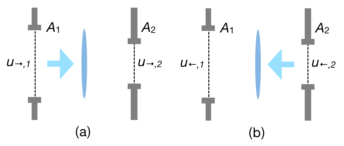
Figure 5: Beam propagation between two apertures in a beam waveguide: (a) from $A_{1}$ to $A_{2}$, (b) from $A_{2}$ to $A_{1}$. There can be phase modifiers between the two apertures.

In what follows the condition of the theorem is described. Since the resultant field can be determined by the input field, we can write

$$u_{\rightarrow,{2}}=\mathcal{P}_{1\rightarrow 2}(u_{\rightarrow,{1}}),\quad\text{and}\quad u_{\leftarrow,{1}}=\mathcal{P}_{1\leftarrow 2}(u_{\leftarrow,{2}})$$ (33)

where $\mathcal{P}_{1\rightarrow 2}$ and $\mathcal{P}_{1\leftarrow 2}$ are operators that converts the input field on one aperture to the resultant field on the other. Let us introduce a notation representing a surface integral of two beam fields $v$ and $w$:

$$\begin{split}\langle v,w\rangle_{1}&:=\int_{P_{1}}v(p)w^{*}(p)\mathrm{d}^{2}p,\\ \langle v,w\rangle_{2}&:=\int_{P_{2}}v(p)w^{*}(p)\mathrm{d}^{2}p.\end{split}$$ (34)

We consider only beams with a finite power passing through a finite aperture, and thus the integrals have a finite value. Two properties of the propagation operators $\mathcal{P}_{1\rightarrow 2}$ and $\mathcal{P}_{1\leftarrow 2}$ are considered: the energy conservation

$$\langle v,w\rangle_{1}=\langle\mathcal{P}_{1\rightarrow 2}(v),\mathcal{P}_{1\rightarrow 2}(w)\rangle_{2}$$ (35)

and the time reversal symmetry

$$\mathcal{P}_{1\rightarrow 2}(v^{*})=\mathcal{P}_{1\leftarrow 2}^{-1}(v)^{*}$$ (36)

for any beam field $v$ and $w$. If the propagation operators $\mathcal{P}_{1\rightarrow 2}$ and $\mathcal{P}_{1\leftarrow 2}$ which satisfies (35) and (36) relates the input fields $u_{\rightarrow,{1}}$ and $u_{\leftarrow,{2}}$ and the resultant fields $u_{\rightarrow,{2}}$ and $u_{\leftarrow,{1}}$ by (33), then

$$\langle u_{\rightarrow,{1}},u_{\leftarrow,{1}}^{*}\rangle_{1}=\langle u_{\rightarrow,{2}},u_{\leftarrow,{2}}^{*}\rangle_{2}.$$ (37)

This equation is equivalent to (32).

Here is the proof of (37).

$$\begin{split}\langle u_{\rightarrow,{1}},u_{\leftarrow,{1}}^{*}\rangle_{1}&=\langle\mathcal{P}_{1\rightarrow 2}(u_{\rightarrow,{1}}),\mathcal{P}_{1\rightarrow 2}(u_{\leftarrow,{1}}^{*})\rangle_{2}\\ &=\langle u_{\rightarrow,{2}},\mathcal{P}_{1\rightarrow 2}(u_{\leftarrow,{1}}^{*})\rangle_{2}\\ &=\langle u_{\rightarrow,{2}},\mathcal{P}_{1\leftarrow 2}^{-1}(u_{\leftarrow,{1}})^{*}\rangle_{2}\\ &=\langle u_{\rightarrow,{2}},u_{\leftarrow,{2}}^{*}\rangle_{2},\end{split}$$

where the first equality follows from (35), the second from the first equation of (33), the third from (36), and the last from the second equation of (33).

Now let us confirm that the propagation through a lossless beam waveguide satisfies the condition (35) and (36). The propagation through a lossless beam waveguide can be decomposed into two kinds of operation: beam propagation in a uniform media or vacuum from a plane to another plane and modification of beam phase.

Beam propagation is governed by the Helmholtz equation and can be described by the Rayleigh-Sommerfeld diffraction, the Fresnel diffraction, or the Fraunhofer diffraction, according to the approximation used [18]. In any case, the energy conservation and the time reversal symmetry hold.

Beam phase modification is implemented by lens or curved mirrors. In this case, the apertures $A_{1}$ and $A_{2}$ are taken at just before and after the element which modifies the beam phase. The effect of the element can be expressed using a function $m(p)$ as

$$u_{\rightarrow,{2}}(p)=m(p)u_{\rightarrow,{1}}(p)\ \text{and}\ u_{\leftarrow,{1}}(p)=m(p)u_{\leftarrow,{2}}(p),$$ (38)

where $|m(p)|^{2}=1$. Then, the operators representing the phase modification by the element $\mathcal{M}_{1\rightarrow 2}$ and $\mathcal{M}_{1\leftarrow 2}$ are $(\mathcal{M}_{1\rightarrow 2}(v))(p)=m(p)v(p)$ and $(\mathcal{M}_{1\leftarrow 2}(w))(p)=m(p)w(p)$, respectively. We can prove the energy conservation of $\mathcal{M}_{1\rightarrow 2}$ as follows.

$$\begin{split}\langle\mathcal{M}_{1\rightarrow 2}(v),\mathcal{M}_{1\rightarrow 2}(w)\rangle_{2}&=\int_{P_{2}}m(p)^{*}v(p)^{*}m(p)w(p)\mathrm{d}^{2}p\\ &=\int_{P_{1}}v(p)^{*}w(p)\mathrm{d}^{2}p\\ &=\langle v,w\rangle_{1}.\end{split}$$

The time reversal symmetry of $\mathcal{M}_{1\rightarrow 2}$ and $\mathcal{M}_{1\leftarrow 2}$ can be shown as follows.

$$\begin{split}(\mathcal{M}_{1\rightarrow 2}(w))(p)^{*}&=m(p)^{*}w(p)^{*}\\ &=w(p)^{*}/m(p)\\ &=(\mathcal{M}_{1\leftarrow 2}^{-1}(w^{*}))(p).\end{split}$$

Therefore both the kinds of operators satisfy the condition (35) and (36). We can easily see that when two operators satisfy the condition, then their composition also satisfies the condition. This completes the proof of the theorem.

M. Nagai received the M.S. degrees in physics from the University of Tokyo in 2005 and the Ph.D. degree in physics from the University of Tokyo in 2008. From 2010 to 2012, he was a researcher in Institute of Particle and Nuclear Studies, High Energy Accelerator Research Organization (KEK). From 2012 to 2017, he was with Observational Astrophysics Laboratory, University of Tsukuba. Since 2017, he has been a Specially Appointed Research Staff of Advanced Technology Center, NAOJ. His research interests include radio astronomy, observational cosmology, design of radio telescopes, characterization and calibration methods for radio telescopes.

H. Imada received the M.S. degrees in physics from University of Tsukuba in 2013 and the Ph.D. degree in physics from University of Tsukuba in 2016. From 2016 to 2018, he was a researcher in Institute of Space and Astronautical Science (ISAS), Japan Aerospace Exploration Agency (JAXA). From 2018 to 2020, he was a researcher in Université Paris-Saclay, CNRS/IN2P3, IJCLab in Orsay, France, formerly Laboratoire de l’Accélérateur Linéaire (LAL). He moved to Kavli Institute for Physics and Mathematics of the Universe (WPI), The University of Tokyo Institutes for Advanced Study, The University of Tokyo, in 2020. He has moved to NAOJ as an antenna scientist in the ALMA project since October, 2020. His research interests include observational cosmology, optical theory for a radio telescope, and numerical simulation of an optical system.

T. Okumura received the M.S. degrees in physics from University of Tsukuba in 2017 and the Ph.D. degree in physics from University of Tsukuba in 2020.

References

- [1] K. Kohno, Y. Tamura, A. Inoue, R. Kawabe, T. Oshima, B. Hatsukade, T. Takekoshi, Y. Yoshimura, H. Umehata, H. Dannerbauer, C. Cicone, and F. Bertoldi, “Exploration and characterization of the earliest epoch of galaxy formation: beyond the re-ionization era,” Astro2020: Decadal Survey on Astronomy and Astrophysics, vol. 2020, p. 402, May 2019.
- [2] H. Dannerbauer, E. van Kampen, J. Afonso, P. Andreani, F. A. Battaia, F. Bertoldi, C. Casey, C.-C. Chen, D. L. Clements, C. De Breuck, B. Frye, J. Geach, K. Harrington, M. Hayashi, S. Jin, P. Klaassen, K. Kohno, M. D. Lehnert, I. Matute, T. Mroczkowski, A. Noble, C. Pappalardo, Y. Tamura, and J. Zavala, “Mapping Galaxy Clusters in the Distant Universe,” BAAS, vol. 51, no. 3, p. 293, May 2019.
- [3] J. Geach, M. Banerji, F. Bertoldi, M. Bethermin, C. M. Casey, C.-C. Chen, D. L. Clements, C. Cicone, F. Combes, C. Conselice, A. Cooray, K. Coppin, E. Daddi, H. Dannerbauer, R. Dave, M. Doherty, J. S. Dunlop, A. Edge, D. Farrah, M. Franco, G. Fuller, T. Garratt, W. Gear, T. R. Greve, E. Hatziminaoglou, C. C. Hayward, R. J. Ivison, R. Kawabe, P. Klaassen, K. K. Knudsen, K. Kohno, M. Koprowski, C. D. P. Lagos, G. E. Magdis, B. Magnelli, S. L. McGee, M. Michalowski, T. Mroczkowski, O. Noroozian, D. Narayanan, S. Oliver, D. Riechers, W. Rujopakarn, D. Scott, S. Serjeant, M. W. L. Smith, M. Swinbank, Y. Tamura, P. van der Werf, E. van Kampen, A. Verma, J. Vieira, J. Wagg, F. Walter, L. Wang, A. Wootten, and M. S. Yun, “The case for a ’sub-millimeter SDSS’: a 3D map of galaxy evolution to z 10,” BAAS, vol. 51, no. 3, p. 549, May 2019.
- [4] K. Abazajian, G. Addison, P. Adshead, Z. Ahmed, S. W. Allen, D. Alonso, M. Alvarez, A. Anderson, K. S. Arnold, C. Baccigalupi, K. Bailey, D. Barkats, D. Barron, P. S. Barry, J. G. Bartlett, R. Basu Thakur, N. Battaglia, E. Baxter, R. Bean, C. Bebek, A. N. Bender, B. A. Benson, E. Berger, S. Bhimani, C. A. Bischoff, L. Bleem, S. Bocquet, K. Boddy, M. Bonato, J. R. Bond, J. Borrill, F. R. Bouchet, M. L. Brown, S. Bryan, B. Burkhart, V. Buza, K. Byrum, E. Calabrese, V. Calafut, R. Caldwell, J. E. Carlstrom, J. Carron, T. Cecil, A. Challinor, C. L. Chang, Y. Chinone, H.-M. S. Cho, A. Cooray, T. M. Crawford, A. Crites, A. Cukierman, F.-Y. Cyr-Racine, T. de Haan, G. de Zotti, J. Delabrouille, M. Demarteau, M. Devlin, E. Di Valentino, M. Dobbs, S. Duff, A. Duivenvoorden, C. Dvorkin, W. Edwards, J. Eimer, J. Errard, T. Essinger-Hileman, G. Fabbian, C. Feng, S. Ferraro, J. P. Filippini, R. Flauger, B. Flaugher, A. A. Fraisse, A. Frolov, N. Galitzki, S. Galli, K. Ganga, M. Gerbino, M. Gilchriese, V. Gluscevic, D. Green, D. Grin, E. Grohs, R. Gualtieri, V. Guarino, J. E. Gudmundsson, S. Habib, G. Haller, M. Halpern, N. W. Halverson, S. Hanany, K. Harrington, M. Hasegawa, M. Hasselfield, M. Hazumi, K. Heitmann, S. Henderson, J. W. Henning, J. C. Hill, R. Hlozek, G. Holder, W. Holzapfel, J. Hubmayr, K. M. Huffenberger, M. Huffer, H. Hui, K. Irwin, B. R. Johnson, D. Johnstone, W. C. Jones, K. Karkare, N. Katayama, J. Kerby, S. Kernovsky, R. Keskitalo, T. Kisner, L. Knox, A. Kosowsky, J. Kovac, E. D. Kovetz, S. Kuhlmann, C.-l. Kuo, N. Kurita, A. Kusaka, A. Lahteenmaki, C. R. Lawrence, A. T. Lee, A. Lewis, D. Li, E. Linder, M. Loverde, A. Lowitz, M. S. Madhavacheril, A. Mantz, F. Matsuda, P. Mauskopf, J. McMahon, M. McQuinn, P. D. Meerburg, J.-B. Melin, J. Meyers, M. Millea, J. Mohr, L. Moncelsi, T. Mroczkowski, S. Mukherjee, M. Münchmeyer, D. Nagai, J. Nagy, T. Namikawa, F. Nati, T. Natoli, M. Negrello, L. Newburgh, M. D. Niemack, H. Nishino, M. Nordby, V. Novosad, P. O’Connor, G. Obied, S. Padin, S. Pandey, B. Partridge, E. Pierpaoli, L. Pogosian, C. Pryke, G. Puglisi, B. Racine, S. Raghunathan, A. Rahlin, S. Rajagopalan, M. Raveri, M. Reichanadter, C. L. Reichardt, M. Remazeilles, G. Rocha, N. A. Roe, A. Roy, J. Ruhl, M. Salatino, B. Saliwanchik, E. Schaan, A. Schillaci, M. M. Schmittfull, D. Scott, N. Sehgal, S. Shandera, C. Sheehy, B. D. Sherwin, E. Shirokoff, S. M. Simon, A. Slosar, R. Somerville, D. Spergel, S. T. Staggs, A. Stark, R. Stompor, K. T. Story, C. Stoughton, A. Suzuki, O. Tajima, G. P. Teply, K. Thompson, P. Timbie, M. Tomasi, J. I. Treu, M. Tristram, G. Tucker, C. Umiltà, A. e. van Engelen, J. D. Vieira, A. G. Vieregg, M. Vogelsberger, G. Wang, S. Watson, M. White, N. Whitehorn, E. J. Wollack, W. L. Kimmy Wu, Z. Xu, S. Yasini, J. Yeck, K. W. Yoon, E. Young, and A. Zonca, “CMB-S4 Science Case, Reference Design, and Project Plan,” arXiv e-prints, p. arXiv:1907.04473, Jul 2019.
- [5] M. Hazumi, P. Ade, Y. Akiba, D. Alonso, K. Arnold, J. Aumont, C. Baccigalupi, D. Barron, S. Basak, S. Beckman et al., “Litebird: A satellite for the studies of b-mode polarization and inflation from cosmic background radiation detection,” Journal of Low Temperature Physics, vol. 194, no. 5-6, pp. 443–452, 2019.
- [6] K. S. Karkare, P. Ade, Z. Ahmed, K. D. Alexander, M. Amiri, D. Barkats, S. Benton, C. A. Bischoff, J. Bock, H. Boenish et al., “Optical characterization of the BICEP3 CMB polarimeter at the South Pole,” in Millimeter, Submillimeter, and Far-Infrared Detectors and Instrumentation for Astronomy VIII, vol. 9914. International Society for Optics and Photonics, 2016, p. 991430.
- [7] “Ieee standard for definitions of terms for antennas,” IEEE Std 145-2013 (Revision of IEEE Std 145-1993), pp. 1–50, March 2014.
- [8] J. D. Kraus, Antennas. New York, McGraw-Hill, 1950.
- [9] C. A. Balanis, Aperture Antennas. In: Antenna theory : analysis and design. NJ: Wiley-Interscience, 2005, pp. 653–738.
- [10] J. W. Baars, Antenna characteristics in practical applications. In: The Paraboloidal Reflector Antenna in Radio Astronomy and Communication: Theory and Practice. New York, NY: Springer New York, 2007, pp. 55–108. [Online]. Available: https://doi.org/10.1007/978-0-387-69734-5_4
- [11] J. Cheng, Fundamentals of Radio Telescopes In: The Principles of Astronomical Telescope Design. New York, NY: Springer New York, 2009, pp. 339–376. [Online]. Available: https://doi.org/10.1007/b105475_6
- [12] W. L. Stutzman and G. A. Thiele, Aperture Antennas. In: Antenna Theory and Design. New York, John Wiley & Sons, 2013, pp. 344–432.
- [13] P. . Kildal, “Factorization of the feed efficiency of paraboloids and cassegrain antennas,” IEEE Transactions on Antennas and Propagation, vol. 33, no. 8, pp. 903–908, August 1985.
- [14] P. F. Goldsmith, “Radiation patterns of circular apertures with gaussian illumination,” International Journal of Infrared and Millimeter Waves, vol. 8, no. 7, pp. 771–781, Jul 1987. [Online]. Available: http://dx.doi.org/10.1007/BF01013128
- [15] C. Dragone, “A first-order treatment of aberrations in cassegrainian and gregorian antennas,” IEEE Transactions on Antennas and Propagation, vol. 30, no. 3, pp. 331–339, 1982.
- [16] ——, “First-order correction of aberrations in cassegrainian and gregorian antennas,” IEEE Transactions on Antennas and Propagation, vol. 31, no. 5, pp. 764–775, 1983.
- [17] T. Tsuzuki, T. Nitta, H. Imada, M. Seta, N. Nakai, S. Sekiguchi, and Y. Sekimoto, “Design of wide-field Nasmyth optical system for a submillimeter camera,” Journal of Astronomical Telescopes, Instruments, and Systems, vol. 1, no. 2, pp. 1 – 8, 2015. [Online]. Available: https://doi.org/10.1117/1.JATIS.1.2.025002
- [18] M. Born and E. Wolf, Principles of Optics: Electromagnetic Theory of Propagation, Interference and Diffraction of Light, Sixth Edition. Cambridge University Press, Cambridge, 1997.
- [19] P. Goldsmith, Quasioptical Systems: Gaussian Beam Quasioptical Propogation and Applications, ser. IEEE Press Series on RF and Microwave Technology. Wiley, 1998.
- [20] P. Hannan, “Microwave antennas derived from the cassegrain telescope,” IRE Transactions on Antennas and Propagation, vol. 9, no. 2, pp. 140–153, March 1961.
- [21] C. Dragone, “Offset multireflector antennas with perfect pattern symmetry and polarization discrimination,” The Bell System Technical Journal, vol. 57, no. 7, pp. 2663–2684, Sep. 1978.
- [22] K. F. Warnick, “Antenna Efficiency and the Genius of the IEEE Standard for Antenna Terms [Education Column],” IEEE Antennas and Propagation Magazine, vol. 54, no. 4, pp. 236–237, Aug 2012.
- [23] S. Silver, Microwave Antenna Theory and Design, ser. Massachusetts Institute of Technology Radiation Laboratory Series. McGraw-Hill Book Company, 1949.
- [24] S. E. Schwarz, “Efficiency of quasi-optical couplers,” International Journal of Infrared and Millimeter Waves, vol. 5, no. 12, pp. 1517–1525, Dec 1984. [Online]. Available: https://doi.org/10.1007/BF01040503
- [25] M. Ng Mou Kehn and L. Shafai, “Characterization of dense focal plane array feeds for parabolic reflectors in achieving closely overlapping or widely separated multiple beams,” Radio Science, vol. 44, no. 3, 2009. [Online]. Available: https://agupubs.onlinelibrary.wiley.com/doi/abs/10.1029/2008RS003953
- [26] C. Granet, “Designing axially symmetric cassegrain or gregorian dual-reflector antennas from combinations of prescribed geometric parameters,” IEEE Antennas and Propagation Magazine, vol. 40, no. 2, pp. 76–82, 1998.
- [27] TICRA Engineering Consultants, ““Reference Manual for GRASP8”,” 2003.
- [28] J. W. Lamb, “Quasioptical coupling of Gaussian beam systems to large Cassegrain antennas,” International Journal of Infrared and Millimeter Waves, vol. 7, pp. 1511–1536, Oct. 1986.
- [29] H. Imada, M. Nagai, M. Kino, M. Seta, S. Ishii, and N. Nakai, “Condition of optical systems independent of frequency for wide field-of-view radio telescopes,” IEEE Transactions on Terahertz Science and Technology, vol. 5, no. 1, pp. 57–63, Jan 2015.