Motion Planning for Quadrupedal Locomotion: Coupled Planning, Terrain Mapping and Whole-Body Control

Abstract

Planning whole-body motions while taking into account the terrain conditions is a challenging problem for legged robots since the terrain model might produce many local minima. Our coupled planning method uses stochastic and derivatives-free search to plan both foothold locations and horizontal motions due to the local minima produced by the terrain model. It jointly optimizes body motion, step duration and foothold selection, and it models the terrain as a cost-map. Due to the novel attitude planning method, the horizontal motion plans can be applied to various terrain conditions. The attitude planner ensures the robot stability by imposing limits to the angular acceleration. Our whole-body controller tracks compliantly trunk motions while avoiding slippage, as well as kinematic and torque limits. Despite the use of a simplified model, which is restricted to flat terrain, our approach shows remarkable capability to deal with a wide range of non-coplanar terrains. The results are validated by experimental trials and comparative evaluations in a series of terrains of progressively increasing complexity.

I Introduction

Legged robots can deliver substantial advantages in real-world environments by offering mobility that is unmatched by wheeled counterparts. Nonetheless, most legged robots are still confined to structured terrain. One of the main reasons is the difficulty on generating complex dynamic motions while considering the terrain conditions. Due to this complexity, many legged locomotion approaches focus on terrain-blind methods with instantaneous actions [e.g. 1, 2, 3]. These heuristic approaches assume that reactive actions are enough to ensure the robot stability under unperceived terrain conditions. Unfortunately, these approaches cannot tackle all types of terrain, in particular terrains with big discontinuities. Such difficulties have limited the use of legged systems to specific terrain topologies.

Trajectory optimization with contacts has gained attention in the legged robotics community [4, 5, 6]. It aims to overcome the drawbacks of terrain-blind approaches by considering a horizon of future events (e.g. body movements and foothold locations). It could potentially improve the robot stability given a certain terrain. However, in spite of the promising benefits, most of the works are focused on flat conditions or on simulation. For instance, these trajectory optimization methods do not incorporate any terrain-risk model. This model serves to quantify the footstep difficulty and uncertainty. Nonetheless, it is not yet clear how to properly incorporate this model inside a trajectory optimization framework. Reason why terrain models are often used only for foothold planning (decoupled approach) [e.g. 7, 8].

I-A Contribution

To address challenging terrain locomotion, we extend our previous planning method [9] in two ways. First, we propose a novel robot attitude planning method that heuristically adapts trunk orientation while still guaranteeing the robot’s stability. Our approach establishes limits in the angular acceleration that keep the estimated Centroidal Moment Pivot (CMP) inside the support region. With our attitude planner, the robot can cross challenging terrain with height elevation changes. It allows the robot to navigate over stairs and ramps, as shown in the experimental and simulation trials. Second, we propose a terrain model (based on log-barrier functions) that robustly describes feasible footstep locations. This work presents first experimental studies on how both models influence the legged locomotion over challenging terrain. The paper presents an exhaustive comparison of the coupled planning described in this work against a decoupled planning method proposed in [10, 11]. For doing so, we integrate online terrain mapping, state estimation and whole-body control. This article is an extension of earlier results [9] presented at the IEEE International Conference on Robotics and Automation (ICRA) 2017.

The remainder of the paper is structured as follows: after discussing previous research in the field of dynamic whole-body locomotion (Section II) we briefly describe our decoupled planner method, which we use for comparison. Next, we introduce our locomotion framework in Section III. We describe our coupled planning method (Section IV) and how the terrain model is formulated in our trajectory optimization. Section V briefly describes a controller designed for dynamic motions. This controller improves the tracking performance and the robustness of the locomotion by passivity-based control paradigm. In Section VI, VII we evaluate the performance of our locomotion framework, and provide comparison with our decoupled planner, in real-world experimental trials and simulations. Finally, Section VIII summarizes this work.

II Related work

In environments where smooth and continuous support is available (floors, fields, roads, etc.), exact foot placement is not crucial in the locomotion process. Typically, legged robots are free to move with a gaited strategy, which only considers the balancing problem. The early work of Marc Raibert [12] crystallized these principles of dynamic locomotion and balancing. Going beyond the flat terrain, the Spot and SpotMini quadrupeds are a recent extension of this work. While SpotMini is able to traverse irregular terrain using a reactive controller, we believe that (as there is no published work) the footholds are not planned in advance. Similar performance can be seen on the Hydraulically actuated Quadruped (HyQ) robot, that is able to overcome obstacles with reactive controllers [2, 13] and/or step reflexes [14, 15].

The main limitation of those gaited approaches is that they quickly reach the robot limits (e.g. torque limits) in environments with complex geometry: large gaps, stairs or rubble, etc. Furthermore, in these environments, the robot often can afford only few possible discrete footholds. Reason why it is important to carefully select footholds that do not impose a particular gaited strategy. Towards this direction, the DARPA Learning Locomotion Challenge stimulated the development of strategies that handle a variety of terrain conditions. It resulted in a number of successful control architectures [7, 8] that plan [16, 17, 18] and execute footsteps [19] in a predefined set of challenging terrains. Roughly speaking, these approaches are able to compute foothold locations by using tree-search algorithms, and to learn the terrain cost-map from user demonstrations [20].

Legged locomotion can also be formulated as an optimal control problem. However, most works do not consider the contact location and timings [e.g. 21, 22, 23] due to the requirement of having a smooth formulation. The contact location and timings are often planned using heuristic rules with partial guarantee of dynamic feasibility [24, 25]. Using these rules, it is possible to avoid the combinatorial complexity and the excessive computation time of more formal approaches ([e.g. 26, 27, 28, 29]). Even though recent works have reduced the computation time by a few orders of magnitude [e.g. 5, 6], they are still limited to offline planning and they require a convex model of the terrain. In the following subsection, we briefly describe our previous decoupled planning method, which will be used as baseline to compare against our new coupled planning method.

II-A Decoupled planning

In our previous decoupled planning locomotion framework [10, 11], the sequence of footholds was selected by computing an approximate body path. It builds body-state graph that quantifies the cost given a set of primitive actions towards a goal. Then, it chooses locally the locations of the footholds. Finally, it generates a body trajectory that ensures dynamic stability and achieves the planned foothold sequence. For that, we used two fifth-order polynomials to describe the horizontal Center of Mass (CoM) motion. The stable horizontal motion is computed using a cart-table model. For more details the reader can refer to [10, 11].

III Locomotion Framework

Figure 1: Overview of the locomotion framework. Horizontal optimization computes simultaneously the CoM and footholds $(\mathbf{x}_{com}^{d},\mathbf{\dot{x}}_{com}^{d},\mathbf{x}_{sw}^{d},\mathbf{\dot{x}}_{sw}^{d})$ given a terrain cost-map $\mathbf{T}$. The attitude planner adapts the trunk orientation $(\mathbf{R}^{d},\bm{\omega}^{d},\bm{\dot{\omega}}^{d})$ given a terrain height-map $\mathbf{H}$. This results in a stable motion that is tracked by the whole-body controller. The virtual model allows us to compliantly track the desired CoM motion, and the controller computes an instantaneous whole-body motion $(\mathbf{\bm{\ddot{q}}}^{*},\mathbf{\bm{\lambda}}^{*})$ that satisfies all robot constraints. The optimized motion is then mapped into desired feed-forward torques $\mathbf{\bm{\tau}}^{d}$. To address unpredictable events, we use a joint impedance controller with low stiffness which tracks the desired joint commands $(\mathbf{q}^{d}_{j},\mathbf{\dot{q}}_{j}^{d})$. Finally, a state estimator provides an estimation of the trunk pose and twist $(\mathbf{x}_{com},\mathbf{\dot{x}}_{com},\bm{\omega},\bm{\dot{\omega}})$. It uses IMU and kinematics (leg odometry), and stereo vision (visual odometry).

In this section, we give an overview of the main components of our locomotion framework (Section III-B), after a quick description of the HyQ robot (Section III-A).

III-A The HyQ robot

HyQ is a 85 kg hydraulically actuated quadruped robot [30]. It is fully torque-controlled and equipped with precision joint encoders, a depth camera (Asus Xtion), a MultiSense SL sensor and an Inertial Measurement Unit (MicroStrain). HyQ measures approx. 1.0 m$\times$0.5 m$\times$0.98 m (length $\times$ width $\times$ height). The leg extension length ranges from 0.339-0.789 m and the hip-to-hip distance is 0.75 m (in the sagittal plane). It has two onboard computers: a Intel i5 processor with Real Time (RT) Linux (Xenomai) patch, and a Intel i5 processor with Linux. The Xenomai PC handles the low-level control (hydraulic-actuator control) at 1 kHz and communicates with the proprioceptive sensors through EtherCAT boards. Additionally, this PC runs the high-level (whole-body) controller at 250 Hz. Both RT threads (i.e. low- and high- level controllers) communicate through shared memory. On the other hand, the non-RT PC processes the exteroceptive sensors to generate the terrain map and then compute the plans. These motion plans are sent to the whole-body controller (i.e. the RT PC) through a RT-friendly communication.

III-B Framework components

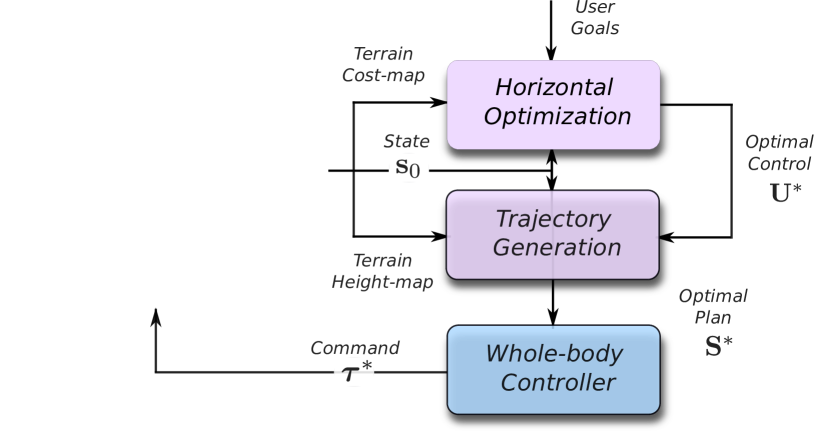
Our locomotion framework is composed by three main modules: motion planning, whole-body control, and mapping and estimation (Fig. 1). The horizon optimization computes the CoM motion and footholds to satisfy robot stability and to deal with terrain conditions (Section IV-C). To handle terrain heights, our attitude planner adapts the trunk orientation as described in Section IV-A1. We build onboard a terrain cost-map and height-map which are used by the horizontal and attitude planners, respectively (Section IV-B).

The whole-body controller has been designed to compliantly track motion plans (Section V). It consists of a virtual model, a joint impedance controller and a whole-body optimization. The virtual model converts a desired motion into a desired wrench. We additionally compensate for gravity to improve motion tracking. Then, a whole-body optimization computes the joint accelerations and the contact forces that satisfy all the robot constraints (torque limits, kinematic limits and friction cone). This output is mapped into desired feed-forward torque commands. To address unpredictable events (e.g. slippage and contact instability), we include a joint impedance controller with low stiffness. Finally, the torque commands are tracked by a torque controller [31].

The state estimation receives updates from proprioceptive sensors (IMU, torque sensors and encoders) as well as from exteroceptive sensors (stereo vision and LiDAR). Faster updates (1 kHz) are obtained using leg odometry [32]. To correct drift, we fused at low frequencies visual odometry: optical flow and LiDAR registration [33]. The terrain mapping builds locally the cost-map and height-map using the depth camera (Asus Xtion). With this, we obtain an accurate trunk position and terrain normals which are needed for the whole-body controller.

IV Motion planning

We consider locomotion to be a coupled planning problem of CoM motions and footholds (see Fig. 2). First, we jointly generate the CoM trajectory and the swing-leg trajectory using a sequence of parametric preview models and the terrain height-map (Section IV-A). Then, in Section IV-C, we optimize a sequence of control parameters, given the terrain cost-map, which defines a horizontal motion of the CoM.

Key novelties, with regards to previous work in [9], are the inclusion of the terrain model in the optimization problem, as a duality cost-constraint, and the development of an attitude planning method. The terrain model allows us to navigate in various terrain conditions without the need for re-tuning. The attitude planner allows the robot to maintain stability in terrain with different elevations. Our coupled planning approach allows us to optimize step timing and to exploit the simplified dynamics for foothold selection, an important improvement from our previous above-mentioned decoupled planning method.

Figure 2: Overview of our coupled motion and foothold planning framework [9]. We compute offline an optimal sequence of control parameters $\mathbf{\bm{U}}^{*}$ given the user’s goals, the actual state $\mathbf{\bm{s}}_{0}$ and the terrain cost-map. Given this optimal control sequence, we generate the optimal plan $\mathbf{\bm{S}}^{*}$, that uses trunk attitude planning to adapt to the changes in the terrain elevation. Lastly, the whole-body controller calculates the joint torques $\bm{\tau}$ that satisfy friction-cone constraints. (Figure from [9].)

IV-A Trajectory generation

We generate the horizontal CoM trajectory and the 2D foothold locations using a sequence of low-dimensional preview models (Section IV-A1). An optimization will provide a sequence of control parameters for these models, that will form the horizontal CoM trajectory. Not specifying the vertical motion for the CoM allows us to decouple the CoM and trunk attitude planning. In a second step, to achieve dynamic adaptation to changes in the terrain elevation, we proposed a novel approach based on the maximum allowed angular accelerations (Section IV-A1).

IV-A1 Preview model

Preview models are low-dimensional (reduced) representations that are useful to describe and capture different locomotion behaviors, such as walking and trotting, and provide an overview of the motion [34, 35]. With a reduced model we can still generate complex locomotion behaviors and their transitions; furthermore, we can integrate it with reactive control techniques. In the literature, different models that capture the legged locomotion dynamics such as point-mass, inverted pendulum, cart-table, or contact wrench have been studied by [36, 37].

Our cart-table with flywheel model (preview model) allows us to decouple the CoM motion from the trunk attitude (Fig. 3). To do not affect the Center of Pressure (CoP) stability condition, we need to keep the CMP inside the support region. With the cart-table model, the horizontal optimization computes a sequence of control that keeps –within a safety margin– the CoP inside the support polygon. The attitude planner corrects the robot orientation in such a way that the CMP position stays inside the support region. This is possible due to the flywheel model allows us to predict the CMP position given the trunk angular acceleration. Note that high centroidal moments (e.g. due to high trunk angular acceleration) can hamper the CoP stability condition e.g. causing that the CMP moves out of the support polygon [38] and making the robot losing its capability to balance.

Figure 3: A trajectory obtained from a low-dimensional model given a sequence of optimized control parameters. The colored spheres represent the CoM and CoP positions of the terminal states of each motion phase. The CoP spheres lie inside the support polygon (same color is used). Note that color indicates the phase (from yellow to red), and the control parameters are computed from the terrain cost-map in grey-scale. The trunk adaptation is based on the estimated support planes in each phase. Since the control parameters are expressed in the horizontal frame (frame that coincides with the base frame but aligned with gravity), the horizontal CoM trajectories and the trunk attitude are decoupled. (Figure from [9])

Horizontal CoM motion

In our previous work [10], we have observed that, in each locomotion phase, the CoP has an approximately linear displacement (see Fig. 8 from [10]), i.e.:

$$\mathbf{\bm{p}}^{H}(t)=\mathbf{\bm{p}}^{H}_{0}+\frac{\delta\mathbf{\bm{p}}^{H}}{T}t,$$ (1)

where $\mathbf{\bm{p}}^{H}=(x^{H},y^{H})\in\mathbb{R}^{2}$ is the horizontal CoP position, $\delta\mathbf{\bm{p}}^{H}\in\mathbb{R}^{2}$ the horizontal CoP displacement and $T$ is the phase duration. The $(\cdot)^{H}$ apex means that the vectors are expressed in the horizontal frame. As shown in [34], it possible, using a cart-table model, to derive an analytical expression for the horizontal CoM trajectory whenever it is assumed a linear displacement of the CoP:

$$\mathbf{\bm{x}}^{H}(t)=\bm{\beta}_{1}e^{\omega t}+\bm{\beta}_{2}e^{-\omega t}+\mathbf{\bm{p}}^{H}_{0}+\frac{\delta\mathbf{\bm{p}}^{H}}{T}t,$$ (2)

where the model coefficients $\bm{\beta}_{1,2}\in\mathbb{R}^{2}$ depend on the actual state $\mathbf{\bm{s}}_{0}$ (horizontal CoM position $\mathbf{\bm{x}}^{H}_{0}\in\mathbb{R}^{2}$ and velocity $\dot{\mathbf{\bm{x}}}^{H}_{0}\in\mathbb{R}^{2}$, and CoP position), the CoM height $h$, the phase duration $T$, and the horizontal CoP displacement $\delta{\mathbf{\bm{p}}}$:

$$\bm{\beta}_{1}=(\mathbf{\bm{x}}^{H}_{0}-\mathbf{\bm{p}}^{H}_{0})/2+(\dot{\mathbf{\bm{x}}}^{H}_{0}T-\delta{\mathbf{\bm{p}}}^{H})/(2\omega T),$$

$$\bm{\beta}_{2}=(\mathbf{\bm{x}}^{H}_{0}-\mathbf{\bm{p}}^{H}_{0})/2-(\dot{\mathbf{\bm{x}}}^{H}_{0}T-\delta{\mathbf{\bm{p}}}^{H})/(2\omega T),$$

with $\omega=\sqrt{g/h}$ and $g$ is the gravity acceleration.

Trunk attitude

The robot requires to adapt its trunk attitude when the terrain elevation varies. As naive heuristic, we could always try to align the trunk with respect to the estimated support plane. However, blindly following the heuristics can lead to big changes in the orientation. In this case big moments might move the CMP out of the support polygon, thus invalidating the CoP condition for stability and making the robot lose control authority. To address this issue, we propose to limit the attitude adaptation by introducing bounds that can guarantee the motion stability. For that, we observe that, for a cart-table with flywheel model, the CMP $\mathbf{\bm{m}}\in\mathbb{R}^{3}$ is linked to the CoP $\mathbf{\bm{p}}\in\mathbb{R}^{3}$  [39, 38] as:

$${\color[rgb]{0,0,0}\mathbf{\bm{m}}=\mathbf{\bm{p}}+\Delta}$$ (3)

where $\Delta$ is the shift resulting from applying moment to the CoM:

$$\Delta_{x} =\tau_{{com}_{y}}/mg,$$ (4)

$$\Delta_{y} ={\color[rgb]{0,0,0}-}\tau_{{com}_{x}}/mg,$$

and $\tau_{com_{y}}$, $\tau_{com_{x}}$ are the horizontal components of the moment about the CoM. Then, thanks to the simplified flywheel model we can also link these moments to angular accelerations of the CoM, i.e. $\bm{\tau}_{com}=\mathcal{I}\dot{\bm{\omega}}$. Re-writing Eq. (4) in vectorial form we have:

$${\color[rgb]{0,0,0}\Delta=\frac{\mathcal{I}\dot{\bm{\omega}}\times{\mathbf{\bm{\hat{e}}}_{z}}}{mg}.}$$ (5)

where $\mathcal{I}\in\mathbb{R}^{3\times 3}$ is the time-invariant inertial tensor approximation (e.g. for a default joint configuration) of the centroidal inertia matrix of the robot, and $\mathbf{\bm{\hat{e}}}_{z}$ is z basis vector of the inertial frame.

Under the flywheel assumption, we can keep the CMP inside the support polygon by limiting the angular acceleration of the trunk to $\dot{\bm{\omega}}_{max}$, where this value is computed from a safety margin $r$ defined in the trajectory optimization (see Section IV-C3) as:

$$r={\color[rgb]{0,0,0}\Big{\|}\frac{(\mathcal{I}\dot{\bm{\omega}}_{max})\times{\mathbf{\bm{\hat{e}}}_{z}}}{mg}\Big{\|}.}$$ (6)

With this, we can adapt the trunk attitude without affecting the stability of the robot. To summarize we want to align the trunk to the estimated support plane. However, the level of alignment is limited by the maximum allowed angular accelerations, in the frontal and the transverse plane (i.e. $\dot{\omega}_{x}$ and $\dot{\omega}_{y}$), computed from Eq. (6) given a user-defined $r$ margin.

We employ cubic polynomial splines to describe the trunk attitude motion (frontal and transverse). The attitude adaptation can be achieved in more than one phase. Indeed, the required angular displacement may not be possible without exceeding the allowed angular accelerations.

Trunk height

We do not consider vertical dynamics during the CoM generation, instead we assume that the trunk height is constant throughout the motion. For non-coplanar footholds, we use an estimate of the support area which provides the height of the CoP point. With this, the sequence of parameters expressed in the horizontal plane are still valid, i.e. they do not affect the robot stability.

IV-A2 Preview schedule

Describing legged locomotion is possible using a sequence of different preview models — a preview schedule. Using this, we can define different foothold sequences by enabling or disabling different phases in our optimization process, i.e. with phase duration equals zero $(T_{i}=0)$. In the preview schedule, we build up a sequence of control parameters $\mathbf{U}$ from stance $\mathbf{\bm{u}}^{st}$ and foot-swing $\mathbf{\bm{u}}^{sw}_{i}$ phases as follows:

$$\mathbf{\bm{U}}=\begin{bmatrix}\mathbf{\bm{u}}^{st/sw}_{1}&\cdots&\mathbf{\bm{u}}^{st/sw}_{n}\end{bmatrix},$$ (7)

in which the phases are defined as $\mathbf{\bm{u}}^{st}_{i}=\begin{bmatrix}T_{i}&\delta\mathbf{\bm{p}}^{H}_{i}\end{bmatrix}$ stance phase where all legs are on the ground and $\mathbf{\bm{u}}^{sw}_{i}=\begin{bmatrix}T_{i}&\delta\mathbf{\bm{p}}^{H}_{i}&\delta\mathbf{\bm{f}}^{l}_{i}\end{bmatrix}$, swing phase, where at least one leg is in swing. $n$ is the number of phases, $l$ is the swing foot, $T_{i}$ is the phase duration and $\delta\mathbf{\bm{f}}_{i}^{l}$ is the relative foothold location (i.e. foot-shift) described w.r.t. the stance frame (Fig. 4). The stance frame is computed from a default posture of the robot. Note that the foothold locations do not affect the CoM dynamics since our model neglects the leg masses and the angular dynamics (cart-table model). In addition, due to the fact that the foot location is an optimization variable that affects the shape of the polygon used as stability constraint for the Zero Moment Point (ZMP), we have the product of two optimization variables, hence the problem becomes non-linear.

The horizontal CoM trajectory is computed from a sequence of phase duration and CoP displacements $\{T_{i},\delta\mathbf{\bm{p}}_{i}^{H}\}$, and its height is kept constant according to the estimated support polygon. Note that the trunk attitude adaption depends on the safety margin and the footstep heights (computed from the terrain height-map). In short, the CoM trajectory can be represented as follows:

$${\color[rgb]{0,0,0}\mathbf{\bm{S}}=\{\mathbf{\bm{s}}_{1},\cdots,\mathbf{\bm{s}}_{N}\}=\mathbf{\bm{f}}(\mathbf{\bm{s}}_{0},\mathbf{\bm{U}},r)}$$ (8)

where the preview state $\mathbf{\bm{s}}=\begin{bmatrix}\mathbf{\bm{x}}&\dot{\mathbf{\bm{x}}}&\mathbf{\bm{p}}&\mathbf{\bm{\sigma}}\end{bmatrix}$ is defined by the CoM position and velocity $(\mathbf{\bm{x}},\dot{\mathbf{\bm{x}}})$, CoP position $\mathbf{\bm{p}}$ and the stance support region $\mathbf{\bm{\sigma}}$, which is defined by the active feet described by $\mathbf{U}$. For simplicity, we have described only the initial preview states of each phase in Eq. (8). It is possible to recover any state because $\mathbf{\bm{f}}(\cdot)$ describes the time-continuous CoM dynamics. Using preview models it is important to reduce the number of decision variables (through control parameters).

We are focused on finding a minimum and safer sequence of footsteps given a certain terrain condition. Therefore we need to include the terrain model. A terrain model often is non-convex and not necessary differentiable. If incorporated in an optimization problem this can create plenty of local minima, then stochastic optimization is a promising choice as a solver (more details in Section IV-C). In the following we will provide the description of the terrain model.

Figure 4: Sketch of different variables and frames used in our optimization. The foot-shift $\delta\mathbf{\bm{f}}^{LF}$ is described w.r.t. the stance frame, its bounds are defined by the foothold region (the pink rectangle). The stance frame is calculated from the default posture and expressed w.r.t. the base frame. (Figure modified from [9].)

IV-B Terrain cost-map

Our terrain model is represented by the terrain cost-map. This quantifies how desirable it is to place a foot at a specific location. The cost value for each pixel in the map is computed using geometric terrain features such as height deviation, slope and curvature [40]. These values are computed as a weighted linear combination of the individual features $T(x,y)=\mathbf{\bm{w}}^{T}\mathbf{\bm{T}}(x,y)$, where $\mathbf{\bm{w}}$ and $\mathbf{\bm{T}}(x,y)$ are the weights and feature cost values, respectively. The total cost value is normalized, where 0 and 1 represent the minimum and maximum risk to step in, respectively. The weight vector describes the importance of the different features. Each feature is computed through piece-wise functions that resemble the log-barrier constraint as described in the equations of Section IV-B2, IV-B3. With this, we have extended the off-the-shelf solver to address constrained problems (see Section IV-C for more details). Below the log-barrier function for each feature is described.

IV-B1 Height deviation

The height deviation cost penalizes footholds close to large drop-offs; for instance, this cost is important for crossing gaps or stepping stones. In fact, staying far away from large drop-offs is beneficial because inaccuracies in the execution of footsteps can cause the robot to step into gaps or banned areas. The height deviation feature $f_{h}$ is computed using the standard deviation around a defined neighborhood.

IV-B2 Slope

The slope reflects the local surface normal in a neighborhood around the cell. The normals are computed using Principal Component Analysis (PCA) on the set of nearest neighbors. A high slope value will increase the chance of slipping even in cases where the friction cone is considered, e.g. due to inaccuracies in the friction coefficient or estimated surface normal. Slope cost increases for larger slope values, while small slopes have zero cost as they are approximately flat. We consider the worst possible slope $s_{max}$ occurs when the terrain is very steep (approximately 70^∘).

We map the height deviation and slope features $f$ into cost values through the following piece-wise function:

$$T_{f}(x,y)=\begin{cases}0&f\leq f_{flat}\\ -\ln\Big{(}1-\frac{f(x,y)}{f_{max}-f_{flat}}\Big{)}&f_{flat}<f<f_{max}\\ T_{max}&f\geq f_{max}\end{cases}$$

where $f_{flat}$ is a threshold that defines the flat conditions, $f_{max}$ the maximum allowed feature value, and $T_{max}$ is the maximum cost value. Note that $f_{max}$ defines the barrier of the log function.

IV-B3 Curvature

The curvature describes the contact stability of a given foothold location. For instance, terrain with mild curvature (curvature between $c=6$ to $c=9$) is preferable to flat terrain since it reduces the possibility of slipping, as it has a bowl-like structure. Thus, the cost is equal to zero in those conditions. On the other hand, high and low curvature values represent a narrow crack structure ($c>9=c_{\max}$) or edge structure ($c<-6=c_{\min}$) in which the foot can get stuck in or can slip, respectively. We use the following piece-wise function to compute the cost value from a curvature value $c$:

$$T_{c}(x,y)=\begin{cases}T_{max}-\ln\Big{(}\frac{c(x,y)-c_{\min}}{c_{\max}-c_{\min}}\Big{)}&c_{crack}<c<c_{mild}^{-}\\ 0&c_{mild}^{-}<c<c_{mild}^{+}\\ T_{max}&c\leq c_{crack},\\ \end{cases}$$

where $c_{crack}=-6$, $c_{mild}^{-}=6$, $c_{mild}^{+}=9$ and $c_{\max}=9$. A description of different curvature values can be found in [8]. The barriers are defined by $c_{crack}$ and $c_{mild}$.

IV-C Horizontal trajectory optimization

The trajectory optimization computes an optimal sequence of control parameters $\mathbf{\bm{U}}^{*}$ used for the generation of the horizontal trajectories for the CoM (Section IV-A). We compute the entire plan by solving a finite-horizon trajectory optimization problem for each phase (similarly to a receding horizon strategy). The horizon is described by a predefined number of preview schedules $N$ with $n$ phases (e.g. our locomotion cycle (schedule) has 6 phases). Our method presents several advantages to address challenging terrain locomotion. It enables the robot to generate desired behaviors that anticipate future terrain conditions, which results in smoother transitions between phases. Note that the optimal solution $\mathbf{\bm{U}}^{*}$ is defined as explained in Section IV-A2.

Compared with [34], our trajectory optimization method 1) uses a terrain cost-map model for foothold selection, 2) defines non-linear inequalities constraints for the CoP position, and 3) guarantees the robot stability against changes in the terrain elevation. Additionally, in contrast to  [34], we have defined a single cost function that tracks desired walking velocities, without enforcing the tracking of a specific step time and distance.

IV-C1 Problem formulation

Given an initial state $\mathbf{\bm{s}}_{0}$, we optimize a sequence of control parameters inside a predefined horizon, and apply only the optimal control of the current phase. Given the desired user commands (trunk velocities), a sequence of control parameters $\mathbf{\bm{U}}^{*}$ are computed solving an unconstrained optimization problem:

$$\mathbf{\bm{U}}^{*}=\operatorname*{\arg\!\min}_{\mathbf{\bm{U}}}\sum_{j}\omega_{j}g_{j}({\color[rgb]{0,0,0}\mathbf{\bm{s}}_{0},\mathbf{\bm{U}},r}).$$ (9)

We solve this trajectory optimization problem using the Covariance Matrix Adaptation Evolution Strategy (CMA-ES) [41]. CMA-ES is capable of handling optimization problems that have multiple local minima and discontinuous gradients. An important feature since the terrain cost-map introduces multiple local minima and gradient discontinuity. We use soft-constraints as these provide the required freedom to search in the landscape of our optimization problem. The cost functions or soft-constraints ${\color[rgb]{0,0,0}g_{j}(\mathbf{\bm{s}}_{0},\mathbf{\bm{U}},r)}$ describe: 1) the user command as desired walking velocity and travel direction, 2) the energy, 3) the terrain cost, 4) a soft-constraint to ensure stability (i.e. the CoP condition), and 5) a soft-constraint that ensures the coupling between the horizontal and vertical dynamics, where the horizontal dynamics are described by Eq. (2).

IV-C2 Cost functions

We use the average walking velocity to track the user velocity command. We evaluate the desired velocity command for the entire planning horizon $Nn$ as follows:

$$g_{velocity}=\bigg{(}\dot{\mathbf{\bm{x}}}^{H}_{desired}-\frac{\mathbf{\bm{x}}^{H}_{Nn}-\mathbf{\bm{x}}^{H}_{0}}{\sum_{i=1}^{Nn}{\color[rgb]{0,0,0}T_{i}}}\bigg{)}^{2},$$ (10)

where $\dot{\mathbf{\bm{x}}}^{H}_{desired}\in\mathbb{R}^{2}$ is the desired horizontal velocity, $\mathbf{\bm{x}}^{H}_{Nn}$ is the terminal CoM position, $\mathbf{\bm{x}}^{H}_{0}$ is the actual CoM position, and $T_{i}$ is the duration of $i^{th}$ phase. Note that $\mathbf{\bm{x}}^{H}_{Nn}$ is the latest state that we consider in the planning horizon.

We use an estimated measure of the energy needed to move the robot from one place to another which we call the Estimated Locomotion Cost (ELC). Minimizing the ELC reduces the energy consumption for traversing a given terrain. Since joint torques and velocities are not available in our optimization, we approximate the robot kinetic energy with a single point-mass system (i.e. $\mathcal{K}=\frac{1}{2}m\dot{\mathbf{\bm{x}}}^{2}$). Thus, we compute the total cost along the phases by:

$$g_{elc}=\sum_{i=1}^{Nn}ELC(\dot{\mathbf{\bm{x}}}),$$ (11)

where $ELC(\dot{\mathbf{\bm{x}}})\triangleq\frac{\mathcal{K}}{mgd}$ with $d$ equal to the travel distance in the $xy$ plane.

IV-C3 Soft-constraints

To negotiate different terrains (Fig. 5), we compute onboard the cost-map as described in Section IV-B. Thus, given a foot-shift and CoM position, we can obtain the cost at the correspondent foothold location $(x,y)$ as:

$$g_{terrain}=\mathbf{\bm{w}}^{T}\mathbf{\bm{T}}(x,y),$$ (12)

where $\mathbf{\bm{w}}$ and $\mathbf{\bm{T}}(x,y)$ are the weights and the vector of cost values of every feature at the location $(x,y)$, respectively. Note that each feature is computed as explained in Section IV-B, and they define log-barrier constraints on the terrain. We use a cell grid resolution of 2 cm, a half of the robot’s foot size. As in [11], we demonstrated that this coarse map is a good trade-off in terms of computation time and information resolution for foothold selection. We cannot guarantee convexity in the terrain costmap, which has to be considered in our optimization process.

As mentioned in Section IV-A1, in order to ensure a certain motion freedom for the control of the attitude, we keep the CoP trajectory inside a polygon that it is shrunk by a margin $r$ with respect to the support polygon. We use a set of non-linear inequality constraints to describe the shrunk support region:

$$\mathbf{\bm{L}}(\mathbf{\bm{\sigma}}{\color[rgb]{0,0,0},r})^{T}\begin{bmatrix}\mathbf{\bm{p}}\\ 1\end{bmatrix}>\mathbf{\bm{0}},$$ (13)

where $\mathbf{\bm{L}}(\cdot)\in\mathbb{R}^{l\times 3}$ are the coefficients of the $l$ lines, $\mathbf{\bm{\sigma}}$ the support region defined from the foothold locations, and $\mathbf{\bm{p}}$ the CoP position. Note that it is a nonlinear constraint as we include the foothold positions as decision variables.

Due to the cart-table model assumes a constant height, the consistency between the CoM and CoP motion is ensured by imposing the following soft-constraint:

$$h=\|\mathbf{\bm{x}}-\mathbf{\bm{p}}\|$$ (14)

where $h$ is the cart-table height that describes the default height of the robot, and $\mathbf{\bm{x}}$ and $\mathbf{\bm{p}}$ are the CoM and CoP positions, respectively. This soft-constraint penalizes the artificial increment of the CoM horizontal position that appears when the decoupling with the vertical motion becomes inaccurate (see Eq. (2)).

We impose both soft-constraints (i.e. Eq. (13), (14)) only in the initial and terminal state of each phase. This is sufficient because the stability and the coupling will be guaranteed in the entire phase too. Note that, for the stability constraint, the support polygon remains a convex hull as the possible foothold locations cannot cross its geometric center. We ensure this by limiting the foothold search region, i.e. by bounding the foot-shift (see Fig. 4). These soft-constraints are described using quadratic penalization.

Figure 5: A cost-map allows the robot to negotiate different terrain conditions while following the desired user commands. The cost-map is computed from onboard sensors as described in Section IV-B. The cost values are continuous and represented in color scale, where blue is the minimum and red is the maximum cost. (Figure from [9].)

V Whole-body controller

The tracking of the reference trajectories for the CoM ($\mathbf{\bm{x}}_{com}^{d},\mathbf{\bm{\dot{x}}}_{com}^{d},\mathbf{\bm{\ddot{x}}}_{com}^{d}$), the trunk orientation ($\boldsymbol{R}^{d},\boldsymbol{\omega}^{d},\boldsymbol{\dot{\omega}}^{d}$) and the swing motions ($\mathbf{\bm{x}}_{sw}^{d},\mathbf{\bm{\dot{x}}}_{sw}^{d}$) is ensured by a whole-body controller (i.e. trunk controller). This computes the feed-forward joint torques $\mathbf{\bm{\tau}}_{ff}^{d}$ necessary to achieve a desired motion without violating friction, torques ($\mathbf{\bm{\tau}}_{max,min}$) or kinematic limits ($\mathbf{\bm{q}}_{max,min}$). To fulfill these additional constraints we exploit the redundancy in the mapping between the joint space ($\in\mathbb{R}^{n}$) and the body task ($\in\mathbb{R}^{6}$). To address unpredictable events (e.g. limit foot divergence in the case of slippage on an unknown surface), an impedance controller computes in parallel the feedback joint torques $\mathbf{\bm{\tau}}_{fb}$ from the desired joint motion $(\mathbf{q}^{d}_{j},\dot{\mathbf{q}}^{d}_{j})$. This controller receives position/velocity set-points that are consistent with the body motion to prevent conflicts with the trunk controller. In nominal operations the biggest contribution is generated by the feed-forward torques, i.e. by the trunk controller.

This controller has been previously drafted in [5] and subsequently presented in detail in [42]. Our controller extends previous work on whole-body control, in particular [43, 44]. In this section we briefly summarize its main characteristics. We cast the controller as an optimization problem, in which, by incorporating the full dynamics of the legged robot, all of its Degree of Freedoms (DoFs) are exploited to spread the desired motion tasks globally to all the joints.

Although the usage of a reduced model (e.g. a centroidal model) can be convenient for planning purposes, in control, it is important to consider the dynamics of all the joints when dealing with dynamic motions (as shown in Section VI). In these cases, the effect of the leg dynamics is no longer negligible and must be considered to achieve good tracking.

With this whole-body controller, the robot achieves faster dynamic motions in real-time, see [42], when compared with our previous quasi-static controller [15]. The block diagram of the trunk controller is shown in Fig. 1. A virtual model generates the reference centroidal wrench $\mathbf{\bm{W}}_{imp}$ necessary to track the reference trajectories. The problem is formulated as a Quadratic Programming (QP) with the generalized accelerations and contact forces as decision variables, i.e. $\mathbf{x}=[\ddot{\mathbf{q}}^{T},\bm{\lambda}^{T}]^{T}\in\mathbb{R}^{6+n+3n_{l}}$ where $n_{l}$ is the number of end-effectors in contact:

$$\mathbf{x}^{*}=\operatorname*{\arg\!\min}_{\mathbf{x}=(\ddot{\mathbf{q}},\bm{\lambda})} \|\mathbf{\bm{W}}_{com}-\mathbf{\bm{W}}_{com}^{d}\|^{2}_{\mathbf{\bm{Q}}}+\|\mathbf{x}\|_{\mathbf{\bm{R}}}^{2}$$ (15)

s.t. $$\mathbf{M}\ddot{\mathbf{q}}+\mathbf{h}=\mathbf{S}\bm{\tau}+\mathbf{J}_{c}^{T}\bm{\lambda},$$ (dynamics)

$$\mathbf{J}_{c}\ddot{\mathbf{q}}+\dot{\mathbf{J}}_{c}\dot{\mathbf{q}}=\mathbf{0},$$ (stance)

$$\mathbf{R}\bm{\lambda}\leq\mathbf{\mathbf{r}},$$ (friction)

$$\mathbf{\bar{\ddot{q}}}\leq\mathbf{\ddot{q}}\leq\mathbf{\underline{\ddot{q}}},$$ (kinematics)

$$\mathbf{\bar{\bm{\tau}}}\leq\mathbf{M}\ddot{\mathbf{q}}+\mathbf{h}-\mathbf{J}_{c}^{T}\bm{\lambda}\leq\mathbf{\underline{\bm{\tau}}},$$ (torque)

where $\mathbf{M}$ is the joint-space inertial matrix, $\mathbf{J}_{c}$ is the contact Jacobian, $\mathbf{h}$ is the force vector that accounts Coriolis, centrifugal, and gravitational forces, $(\mathbf{R},\mathbf{r})$ describe the linearized friction cone, $(\mathbf{\bar{\ddot{q}}},\mathbf{\underline{\ddot{q}}})$ are acceleration bounds defined given the current robot configuration [42], and $(\mathbf{\bar{\bm{\tau}}},\mathbf{\underline{\bm{\tau}}})$ describe the torque limits.

The first term of the cost function (15) penalizes the tracking error at the wrench level, while the second one is a regularization factor to keep the solution bounded or to pursue additional criteria. Both costs are quadratic-weighted terms. All the constraints are linear: the equality constraints encode dynamic consistency, the stance condition and the swing task. While the inequality constraints encode friction, torque, and kinematic limits. Then the optimal acceleration and forces $\mathbf{x}^{*}$ are mapped into desired feed-forward joint torques $\bm{\tau}_{ff}^{d}\in\mathbb{R}^{n}$ using the actuated part of the full dynamics. Finally, the feed-forward torques $\bm{\tau}_{ff}^{d}$ are summed with the joint PD torques (i.e. feedback torques $\bm{\tau}_{fb}$) to form the desired torque command $\bm{\tau}^{d}$, which is sent to a low-level joint-torque controller.

A terrain mapping module provides, as inputs to the whole-body controller, an estimate of the friction coefficient $\mu$ and of the normal to the terrain $\hat{n}_{t}$ at each contact location [45]. Finally a state estimation module fuses inertial, visual and odometry information to get the current floating-base position and velocity w.r.t. the inertial frame [33].

VI Experimental Results

To understand the advantages of our locomotion framework, we first compare the decoupled and coupled approaches in different challenging terrains (e.g. stepping stones, pallet, stairs and gap). We use as test-cases for the comparison the decoupled planner presented in [10]. After that, we show how the modulation of the trunk attitude handles heights variations in the terrain. Subsequently, we analyze the effect of the terrain cost-map in our coupled planner. We study how different weighting choices result in different behaviors without affecting significantly the robot stability and the ELC. Finally we demonstrate the capabilities of our complete locomotion framework (i.e. coupled planner, whole-body controller, terrain mapping and state estimation) by crossing terrains with various slopes and obstacles. All the experimental results are in the accompanying video or in Youtube.

VI-A Motion planning: decoupled vs coupled approach

TABLE I: Number of footholds, average walking speed and normalized ELC for different challenging terrains without changes in the elevation for our coupled (Coup.) and decoupled (Dec.) planners. We normalize the ELC with respect to the walking velocity to easily compare results across different motion speeds. All the results are computed from simulations.

	# of Footholds				Avg. Speed [cm/s]				ELC / speed [s/cm]
Terrain	Coup.	Dec.	Ratio		Coup.	Dec.	Ratio		Coup.	Dec.	Ratio
S. Stones	31	38	0.82		11.16	6.29	1.77		13.20	11.43	1.15
Pallet	35	36	0.97		9.23	6.92	1.33		13.21	11.70	1.13
Stairs	21	23	0.91		12.79	11.26	1.14		10.22	6.24	1.63
Gap	18	24	0.75		12.76	9.00	1.42		9.05	6.84	1.32

Figure 6: Snapshots of experimental trials used to evaluate the performance of our trajectory optimization framework. (a) crossing a gap of 25 cm length while climbing up 6 cm. (b) crossing a gap of 25 cm length while climbing down 12 cm. (c) crossing a set of 7 stepping stones. (d) crossing a sparse set of stepping stones with different elevations (6 cm). To watch the video, click the figure.

VI-A1 Decoupled planner setup

The swing and stance duration are predefined since they cannot be optimized. The footstep planner explores partially a set of candidate footholds using the terrain-aware heuristic function [11]. These duration are tuned for every terrain and, range from 0.5 to 0.7 s and from 0.05 to 1.4 s for the swing and stance phases, respectively. However, it is not always possible to compute a set of polynomial’s coefficients (CoM trajectory) that satisfies the dynamic stability for some footstep sequences. Thus, unfortunately, step and swing duration need to be hand-tuned depending on the footstep sequence itself.

VI-A2 Coupled planner setup

The same weight values for the cost functions are used for all the results presented in Table I (i.e. 300, 30 and 10 for the human velocity commands, terrain, and energy, respectively). We did not re-tune these weights for a different experiment, as it was sometimes necessary with the decoupled planner. This shows a greater generality with respect to the decoupled planner. We add a quadratic penalization, when the terrain cost $\mathbf{T}(x,y)$ is higher then 0.8 (i.e. 80% of its maximum value).

For this kind of problems, it is not trivial to define a good initialization trajectory (i.e. to warm-start the optimizer). However, since our solver uses stochastic search, this is not so critical and we decided not to do it. We used the same stability margin and angular acceleration (as in Section VI-B) for the trunk attitude planner, and the horizon is $N=1$, i.e. 1 locomotion cycle or 4 steps.

VI-A3 Increment of the success rate

The foothold error is on average around 2 cm, half than in the decoupled planner case. Note that these results are obtained with the state estimation algorithm proposed in [33]. The coupled planner dramatically increases the success of the stepping stones trials to 90%; up over 30% with respect to the decoupled planner [10]. We define as success when the robot crosses the terrain, e.g. it does not make a step in the gap, and does not reach its torque and kinematic limits. In Table I we report the number of footholds, the average trunk speed, and the ELC for simulations made with our coupled and decoupled planners in different challenging terrains. The coupled planner also increases the walking velocity of least 14% and up to 63%, while also modulating the trunk attitude. The number of footholds is also reduced of 14% on average. Jointly optimizing the motion and footholds reduces the number of steps because it considers the robot dynamics for the foothold selection. Note that the trunk speed and the success rate increased even with terrain elevation changes (e.g. gap and stepping stones). The ELC is higher for our coupled planner; however, this is an effect of higher walking velocities and of the tuning of the cost function. This is expected even if we normalized the ELC with respect to the walking velocity. Note that as velocity increases the kinetic energy rises quadratically with a consequent affect on the ELC. We also found that the tuning of the ELC cost does not affect the stability and the foothold selection.

VI-A4 Computation time

An important drawback of including the terrain cost-map is that it increases substantially the computation time. In fact for our planners, this increases from 2-3 s to 10-15 min, for more details about the computation time of the decoupled planner see [11]. The main reason is that we use a stochastic search which estimates the gradient (see [41]). Instead, for the decoupled planner, we use a tree-search algorithm (i.e. Anytime Repairing A* (ARA*)) with a heuristic function that guides the solution towards a shortest path, not the safest one, which allows us to formulate the CoM motion planning through a QP program. For more details about the footstep planner, used in the decoupled planning approach, see [11].

VI-A5 Crossing challenging terrains

Trunk attitude adaptation tends to overextend the legs, especially in challenging terrains, as bigger motions are required. To avoid kinematic limits, we define a foot search region. This ensures kinematic feasibility for terrain height difference of up to 12 cm (coupled planner), in Fig. 6a, b. Note that in the decoupled case we had to define a more conservative foot search region (i.e. in the footstep planner) than in the coupled one, making very challenging to cross gaps or stepping stones with height variations. Indeed, crossing the terrain in Fig. 6a-d is only possible using the coupled planner since we managed to increase the foothold region from (20 cm$\times$23.5 cm) to (34 cm$\times$28 cm). Note that the decoupled planning requires smaller foothold regions due to the fact that only considers the robot’s kinematics.

For all our optimizations, we define a stability margin of $r=$0.1 m (introduced in Section IV-A1) which is a good trade-off between modeling error and allowed trunk attitude adjustment.

VI-B Trunk attitude planning

The cart-table model neglects the angular dynamics and therefore cannot be used to control the robot’s attitude. However, with a flywheel extension as proposed for our attitude planning approach, we could generate stable motions while changing the robot attitude (e.g. stair climbing as in Fig. 7). In this section, we showcase the automatic trunk attitude modulation during a dynamic walk on the HyQ robot (Fig. 8a).

Figure 7: An optimized sequence of control parameters for stair climbing. As in previous experiments, we use the same optimization weight values for the entire course of the motion. The step heights are 14 cm. To watch the video, click the figure.

To experimentally validate the attitude modulation method, we plan a fast dynamic walk with a trunk velocity of 18 cm/s, and an initial trunk attitude of 0.17 and 0.22 radians in roll and pitch, respectively. We do not use the terrain cost-map to generate the corresponding footholds, thus the resulting feet locations come from the dynamics of walking itself, while maximizing the stability of the gait. We compute the maximum allowed angular acceleration given the trunk inertia matrix of HyQ, from Eq. (6), which results in 0.11 rad/s² as the maximum diagonal element. The trunk attitude planner uses this maximum allowed acceleration to align the trunk and support plane through cubic polynomial splines ( Section IV-A1).

(a) Dynamic walking and trunk modulation

(b) CoM tracking performance

(c) Trunk attitude modulation

Figure 8: (a) Dynamic attitude modulation on the HyQ robot. The initial trunk attitude is 0.17 and 0.22 radians in roll and pitch, respectively. (b) Body tracking when walking and dynamically modulating the trunk attitude. The planned CoM (magenta) and the executed trajectory (white) are shown together with the sequence of support polygons, CoP and CoM positions. Note that each phase is identified with a specific color. (c) A lateral view of the same motion shows the attitude correction (sequence of frames), and the cart-table displacement. We use the RGB color convention for drawing the different frames. In (b)-(c) the brown, yellow, green and blue trajectories represent the Left-Front (LF), Right-Front (RF), Left-Hind (LH) and Right-Hind (RH) foot trajectories, respectively.

Figure 9: The effect of changing terrain weight values when crossing a gap of 25 cm. The cost-map is computed only using the height deviation feature (top); the red points represent the discretization of the continuous cost function (1 cm). The cost values are represented using gray scale, where white and black are the minimum and maximum cost values, respectively. A higher value in the terrain weight describes a higher risk for foothold locations near the borders of the gap. An appropriate weight allows the robot to cross the gap (middle). In contrast, an increment of 200% in the weight penalizes excessively footholds close to the gap and as result the robot cannot cross the gap as kinematic limits are exceeded (bottom).

The resulting behavior shows the HyQ robot successfully walking while changing its trunk roll and pitch angles. The trunk attitude planner adjusts the roll and pitch angles given the estimated support region at each phase. Fig. 8b shows the CoM tracking performance for an initial trunk attitude of 0.17 rad and 0.22 rad in roll and pitch, respectively. Fig. 8c shows that the entire attitude modulation is accomplished in the first 6 phases (i.e. one locomotion cycle or four steps with two support phases). Because our attitude planner keeps the CMP inside the support region, the HyQ robot successfully crosses terrains with different heights as shown in Fig. 6a-d. The stability margin is the same for all the experiments in this paper ($r=0.1$ m).

VI-C Motion planning and terrain mapping

Different weighting choices on the terrain cost-map produce different behaviors, as described by Eq. (12). For simplicity, we analyze the effect of these weights in gap crossing. We observe two different plans which are only influenced by the terrain weight in the cost function (Fig. 9). Strongly penalizing the terrain cost-map results in the robot not being able to cross the gap due to its kinematic limits (Fig. 9(bottom)). By reducing the terrain weight, we observe that the coupled planner selects footholds closer to the gap border, which allows the robot to cross the space (Fig. 9(top)). The terrain weight mainly influences the foothold selection, and does not influence the stability or the ELC. Finally, we observed that the computational cost is not affected by the terrain geometry.

Figure 10: Crossing a terrain that combines elements of the previous cases; first a ramp of $10$ degree, then a gap of 15 cm and finally a step with 15 cm height change. Execution of the planned motion with the HyQ robot (top). Visualization of the terrain cost-map, friction cone and GRFs (bottom). The color for the friction cone and GRFs are magenta and purple, respectively. To watch the video, click the figure.

VI-D Whole-body control, state estimation and terrain mapping

The whole-body controller successfully tracks the planned motion without violating friction, torques or kinematics constraints Fig. 10(bottom). A key aspect is that our controller follows the desired wrenches computed from the motion plan, giving priority to the above constraints. This is important because our coupled planner does not consider the non-coplanar contact condition and friction cone (since the used cart-table model that neglects them). With this approach, the robot can (1) climb in simulation ramps up to $20$ degrees in similar friction conditions to real experiments ($\mu=0.7$) and (2) handle unpredictable contact interactions as shown in Fig. 7.

The terrain surface normals are computed online from vision. The friction coefficient used in these trials (i.e. simulation and experiments) is $0.7$, which is a conservative estimate of the real contact conditions. Fig. 11 shows the tracking performance against errors in the state estimation and terrain mapping. The tracking error is mainly due to low-frequency corrections of the estimated pose.

Figure 11: HyQ crossing a terrain that combines elements of all previous cases. (Top): CoM tracking performance, desired (blue) and executed (black) motions. (Bottom): applied torque command along the course of the motion. At $t=$14 sec, the planned motion produced a movement that reached the torque limits; however, the controller applies a torque command inside the robot’s limits. In fact, the tracking error increases at approximately $x=$1.25 m, and is reduced in the next steps.

VII Discussion

VII-A Motion planning: decoupled vs coupled approach

Coupled motion and foothold planning include dynamics in foothold selection. This is critical to both increase the range of possible foothold locations and to adjust the step duration. Both of these parameters allow the robot to cross a wider range of terrains. We noted that the coupled planner handles different terrain heights more easily because of the joint optimization process. Crossing gaps with various elevations exposed the limitation of decoupled methods, since this is more prune to hit the kinematic limits (see Fig. 6a). However, an important drawback of coupled foothold and motion planning is the increase in computation time compared to decoupled planning. It is possible to reduce the computation time by describing the foothold using integer variables [25, 5], but this would limit the number of feasible convex regions. Instead the coupled planning uses a terrain model that considers a broader range of challenging environments because of the “continuous” cost-map. In any case, the computation time remains longer for coupled planning as we presented in [5].

Optimizing the step timing has not shown a clear benefit in our experimental results. We argue that step timing is important to find feasible solutions when there is a small friction coefficient or the risk of reaching torque limits, i.e. a slower motion is needed to satisfy both constraints. However, the cart-table model does not consider these constraints, which in practice makes the time optimization not useful for reduced dynamics.

We have tested, in simulation, our locomotion framework up to 208 steps on flat terrain (Fig. 12) and up to 50 steps in non-flat terrain (Fig. 7). The modeling errors on the cart-table with flywheel approximation are easily handled by the whole-body controller. In addition, the swing trajectory are expressed in the base frame, so errors in the state estimation affect little the stability. However, unexpected events can compromise the stability (e.g. unstable footsteps, moving obstacles, state estimation errors as a result of slippage, etc) and re-planning might be needed. According to our experience, it is recommended to optimize at least one cycle of locomotion since we do not know the CoM travel direction and velocity in an individual step. For all the experiments, we plan 4 steps ahead and it was not needed a longer horizon. We planned 6 and 8 steps ahead without any significant improvement in the motion. To compute the whole motion, we solve different trajectory optimization problems in receding fashion.

Figure 12: Optimizing 208 steps from 52 trajectory optimization problems. In each optimization problem the step timing, foothold locations and CoM trajectory for 4 steps in advance with different velocity commands are computed. The color describes different step phases of the planned motion.

VII-B Trunk attitude planning

The cart-table model estimates the CoP position, yet it neglects the angular components of the body motion that can lead to inaccuracies in the CoP estimation. This can affect the stability particular when there is a change in height e.g. climbing/descending gaps or stairs, crossing uneven stepping stones, etc. To systematically address these effects without affecting the stability, a relationship was obtained between the torques applied to the CoM and the displacement of the CoP. Later, we connected the stability margin by assuming a time-invariant inertial tensor approximation of the inertia matrix. Experimental results with the HyQ robot validated this method for challenging terrain locomotion. The method developed in this paper can be applied to other legged systems, such as humanoids.

Our attitude planner does not aim to control angular momentum, instead we propose 1) to use a heuristic for trunk orientation and 2) to guarantee the robot stability under mild assumptions. To handle the zero-dynamics instabilities (described in [46]), our whole-body controller tracks the desired robot orientation computed by the trunk attitude planner. However, we argue that a more effective robot attitude planner will require to consider the limb dynamics (full dynamics) and to account for future events (planning). It is clearly crystallized in the cat-falling motion, when the momenta conservation defines a nonholonomic constraint on the angular momentum (for more details see [47]). This is the reason why recent works have been focused on efficient full-body optimization (e.g. [23, 48, 49].

VII-C The effect of the terrain cost-map

Considering the terrain topology increases the complexity of the trajectory optimization problem. Moreover, optimizing the step duration introduces many local minima in the problem landscape. To address these issues, a low-dimensional parameterized model is used which allows us to use stochastic-based search. Note that stochastic-based search becomes quickly intractable when the problem dimension increases. Even though our problem is non-convex, we reduce the number of required footholds by an average of 13.75% compared to our convex decoupled planner (Table I). The terrain cost-map increases the robustness of the planned motion. Indeed, the selected footsteps are far from risky regions, and this is very important to increase robustness because tracking errors always produce variation on the executed footstep.

VII-D Considering terrain with slopes

Higher walking speed increases the probability of foot-slippage. When one or more of the feet slip backwards, or when a foot is only slightly loaded, might result in a poor tracking. Both events are more likely to happen in a terrain with different elevations due to errors in the state estimation or noise in the exteroceptive sensors. Including friction-cone and foot unloading / loading constraints, in the whole-body optimization, has been shown to help mitigate the poor tracking. We demonstrated experimentally that is possible to navigate a wide range of terrain slopes without considering the friction cone stability in the planning level (only at the controller level).

VII-E Terrain mapping and state estimation

Estimating the state of the robot with a level of accuracy suitable for planned motions is a challenging task. Reliable state estimation is crucial, as accurate foot placement directly depends on the robot’s base pose estimate. The estimate is also used to compute the desired torque commands through a virtual model. The major sources of error for inertial-legged state estimation are IMU gyro bias and foot slippage. These produce a pose estimate drift, which cannot be completely eliminated by the contact state estimate [32] (or with proprioceptive sensing). Pose drift particularly affects the desired torques computed from the whole-body optimization. To eliminate it, we fused high frequency (1 kHz) proprioceptive sources (inertial and leg odometry) with low frequency exteroceptive updates (0.5 Hz for LiDAR registration, 10 Hz for optical flow) in a combined Extended Kalman Filter [33]. We noticed that the drift accumulated, in between the high frequency proprioceptive updates and the low frequency exteroceptive updates, affected the experimental performance. In practice, to cope with this problem, we reduced the compliance of our whole-body controller (by increasing the proportional gains).

VIII Conclusion

In this paper, we presented a new framework for dynamic whole-body locomotion on challenging terrain. We extended our previous planning approach from [9] by modeling the terrain through log-barrier functions in the numerical optimization. In addition, we proposed a novel robot attitude planning algorithm. Using this, we could optimize both the CoM motion and footholds in the horizontal frame, and allow the robot to adapt its trunk orientation. We demonstrated in experimental trials and simulations that the assumptions on the attitude planner avoided instability under significant terrain elevation changes (up to 12 $cm$). We compared coupled and decoupled planning and highlighted the advantages and disadvantages of them. In our test-case planners, we used the same method for quantifying the terrain difficulty (i.e. terrain cost-map). We showed that reduced models for motion planning (such as cart-table with flywheel) together with whole-body control are still suitable for a wide range of challenging scenarios. We used the full dynamic model only in our real-time whole-body controller to avoid slippage, and hitting torque and kinematic limits. The online terrain mapping allowed our controller to avoid slippage on the trialled terrain surfaces. We presented results, validated by experimental trials and comparative evaluations, in a series of terrains of progressively increasing complexity.

Carlos Mastalli received the Ph.D. degree on “Planning and Execution of Dynamic Whole-Body Locomotion on Challenging Terrain” from Istituto Italiano di Tecnologia, Genoa, Italy, in April 2017. He is currently a Research Associate in the University of Edinburgh with Alan Turing fellowship. His research combines the formalism of model-base approach with the exploration of vast robot’s data for robot locomotion. From 2017 to 2019, he was a postdoc in the Gepetto Team at LAAS-CNRS. Previously, he completed his Ph.D. on “Planning and Execution of Dynamic Whole-Body Locomotion on Challenging Terrain” in April 2017 at Istituto Italiano di Tecnologia. He is also improved significantly the locomotion framework of the HyQ robot. His has contributions in optimal control, motion planning, whole-body control and machine learning for legged locomotion.

Ioannis Havoutis received the M.Sc. in Artificial Intelligence and Ph.D. in Informatics degrees from the University of Edinburgh, Edinburgh, U.K. He is a Lecturer in Robotics at the University of Oxford. He is part of the Oxford Robotics Institute and a co-lead of the Dynamic Robot Systems group. His focus is on approaches for dynamic whole-body motion planning and control for legged robots in challenging domains. From 2015 to 2017, he was a postdoc at the Robot Learning and Interaction Group, at the Idiap Research Institute. Previously, from 2011 to 2015, he was a senior postdoc at the Dynamic Legged System lab the Istituto Italiano di Tecnologia. He holds a Ph.D. and M.Sc. from the University of Edinburgh.

Michele Focchi received the B.Sc. and M.Sc. degrees in control system engineering from Politecnico di Milano, Milan, Italy, in 2004 and 2007, respectively, and the Ph.D. degree in robotics in 2013. He is currently a Researcher at the Advanced Robotics department, Istituto Italiano di Tecnologia. He received both the B.Sc. and the M.Sc. in Control System Engineering from Politecnico di Milano in 2004 and 2007, respectively. In 2009 he started to develop a novel concept of air-pressure driven micro-turbine for power generation in which he obtained an international patent. In 2013, he got a Ph.D. degree in Robotics, where he developed low-level controllers for the Hydraulically Actuated Quadruped (HyQ) robot. Currently his research interests are dynamic planning, optimization, locomotion in unstructured/cluttered environments, stair climbing, model identification and whole-body control.

Darwin G. Caldwell (Senior Member, IEEE) received the B.Sc. and Ph.D. degrees in robotics from University of Hull, Hull, U.K., in 1986 and 1990, respectively, and the M.Sc. degree in management from University of Salford, Salford, U.K., in 1996. He is a founding Director at the Istituto Italiano di Tecnologia in Genoa, Italy, and a Honorary Professor at the Universities of Sheffield, Manchester, Bangor, Kings College, London and Tianjin University China. His research interests include innovative actuators, humanoid and quadrupedal robotics and locomotion (iCub, HyQ and COMAN), haptic feedback, force augmentation exoskeletons, dexterous manipulators, biomimetic systems, rehabilitation and surgical robotics, telepresence and teleoperation procedures. He is the author or co-author of over 450 academic papers, and 17 patents and has received awards and nominations from several international journals and conferences.

Claudio Semini received a M.Sc. degree in Electrical Engineering and Information Technology from ETH Zurich, Switzerland, in 2005. He is the Head of the Dynamic Legged Systems (DLS) laboratory at Istituto Italiano di Tecnologia (IIT). From 2004 to 2006, he first visited the Hirose Laboratory at Tokyo Tech, and later the Toshiba R&D Center, Japan. During his doctorate from 2007 to 2010 at the IIT, he developed the hydraulic quadruped robot HyQ and worked on its control. After a postdoc with the same department, in 2012, he became the Head of the DLS lab. His research interests include the construction and control of versatile, hydraulic legged robots for real-world environments.

References

- Wensing and Orin [2013] P. M. Wensing and D. E. Orin, “Generation of dynamic humanoid behaviors through task-space control with conic optimization,” in IEEE Int. Conf. Rob. Autom. (ICRA), 2013.
- Barasuol et al. [2013] V. Barasuol, J. Buchli, C. Semini, M. Frigerio, E. R. De Pieri, and D. G. Caldwell, “A Reactive Controller Framework for Quadrupedal Locomotion on Challenging Terrain,” in IEEE Int. Conf. Rob. Autom. (ICRA), 2013.
- Dario Bellicoso et al. [2017] C. Dario Bellicoso, F. Jenelten, P. Fankhauser, C. Gehring, J. Hwangbo, and M. Hutter, “Dynamic locomotion and whole-body control for quadrupedal robots,” in IEEE/RSJ Int. Conf. Intell. Rob. Sys. (IROS), 2017.
- Dai and Tedrake [2016] H. Dai and R. Tedrake, “Planning Robust Walking Motion on Uneven Terrain via Convex Optimization,” in IEEE Int. Conf. Hum. Rob. (ICHR), 2016.
- Aceituno-Cabezas et al. [2017] B. Aceituno-Cabezas, C. Mastalli, H. Dai, M. Focchi, A. Radulescu, D. G. Caldwell, J. Cappelletto, J. C. Grieco, G. Fernandez-Lopez, and C. Semini, “Simultaneous Contact, Gait and Motion Planning for Robust Multi-Legged Locomotion via Mixed-Integer Convex Optimization,” IEEE Robot. Automat. Lett. (RA-L), 2017.
- Winkler et al. [2018] A. W. Winkler, D. C. Bellicoso, M. Hutter, and J. Buchli, “Gait and trajectory optimization for legged systems through phase-based end-effector parameterization,” IEEE Robot. Automat. Lett. (RA-L), vol. 3, 2018.
- Kolter et al. [2008] J. Z. Kolter, M. P. Rodgers, and A. Y. Ng, “A control architecture for quadruped locomotion over rough terrain,” in IEEE Int. Conf. Rob. Autom. (ICRA), 2008.
- Kalakrishnan et al. [2010a] M. Kalakrishnan, J. Buchli, P. Pastor, M. Mistry, and S. Schaal, “Learning, planning, and control for quadruped locomotion over challenging terrain,” The Int. J. of Rob. Res. (IJRR), vol. 30, 2010.
- Mastalli et al. [2017] C. Mastalli, M. Focchi, I. Havoutis, A. Radulescu, S. Calinon, J. Buchli, D. G. Caldwell, and C. Semini, “Trajectory and Foothold Optimization using Low-Dimensional Models for Rough Terrain Locomotion,” in IEEE Int. Conf. Rob. Autom. (ICRA), 2017, pp. 236–258.
- Winkler et al. [2015] A. Winkler, C. Mastalli, I. Havoutis, M. Focchi, D. G. Caldwell, and C. Semini, “Planning and Execution of Dynamic Whole-Body Locomotion for a Hydraulic Quadruped on Challenging Terrain,” in IEEE Int. Conf. Rob. Autom. (ICRA), 2015.
- Mastalli et al. [2015] C. Mastalli, A. Winkler, I. Havoutis, D. G. Caldwell, and C. Semini, “On-line and On-board Planning and Perception for Quadrupedal Locomotion,” in IEEE Conf. on Techn. for Pract. Rob. Apps. (TEPRA), 2015.
- Raibert [1986] M. H. Raibert, Legged robots that balance. MIT press Cambridge, MA, 1986, vol. 3.
- Havoutis et al. [2013] I. Havoutis, J. Ortiz, S. Bazeille, V. Barasuol, C. Semini, and D. G. Caldwell, “Onboard Perception-Based Trotting and Crawling with the Hydraulic Quadruped Robot (HyQ),” in IEEE/RSJ Int. Conf. Intell. Rob. Sys. (IROS), 2013.
- Focchi et al. [2013] M. Focchi, V. Barasuol, I. Havoutis, C. Semini, D. G. Caldwell, V. Barasuol, and J. Buchli, “Local Reflex Generation for Obstacle Negotiation in Quadrupedal Locomotion,” in Int. Conf. on Climb. and Walk. Rob. and the Supp. Techn. for Mob. Mach. (CLAWAR), 2013.
- Focchi et al. [2017] M. Focchi, A. del Prete, I. Havoutis, R. Featherstone, D. G. Caldwell, and C. Semini, “High-slope terrain locomotion for torque-controlled quadruped robots,” Autom. Robots., vol. 41, 2017.
- Pongas et al. [2007] D. Pongas, M. Mistry, and S. Schaal, “A robust quadruped walking gait for traversing rough terrain,” in IEEE Int. Conf. Rob. Autom. (ICRA), 2007.
- Zucker et al. [2011] M. Zucker, N. Ratliff, M. Stolle, J. Chestnutt, J. A. Bagnell, C. G. Atkeson, and J. Kuffner, “Optimization and learning for rough terrain legged locomotion,” The Int. J. of Rob. Res. (IJRR), vol. 30, 2011.
- Shkolnik et al. [2011] A. Shkolnik, M. Levashov, I. R. Manchester, and R. Tedrake, “Bounding on rough terrain with the LittleDog robot,” The Int. J. of Rob. Res. (IJRR), vol. 30, 2011.
- Rebula et al. [2007] J. R. Rebula, P. D. Neuhaus, B. V. Bonnlander, M. J. Johnson, and J. E. Pratt, “A controller for the littledog quadruped walking on rough terrain,” in IEEE Int. Conf. Rob. Autom. (ICRA), 2007.
- Kalakrishnan et al. [2010b] M. Kalakrishnan, J. Buchli, P. Pastor, M. Mistry, and S. Schaal, “Fast, robust quadruped locomotion over challenging terrain,” in IEEE Int. Conf. Rob. Autom. (ICRA), 2010.
- Carpentier and Mansard [2018] J. Carpentier and N. Mansard, “Multi-contact Locomotion of Legged Robots,” IEEE Trans. Robot. (TRO), 2018.
- Ponton et al. [2016] B. Ponton, A. Herzog, S. Schaal, and L. Righetti, “A Convex Model of Momentum Dynamics for Multi-Contact Motion Generation,” in IEEE Int. Conf. Hum. Rob. (ICHR), 2016.
- Budhiraja et al. [2018] R. Budhiraja, J. Carpentier, C. Mastalli, and N. Mansard, “Differential Dynamic Programming for Multi-Phase Rigid Contact Dynamics,” in IEEE Int. Conf. Hum. Rob. (ICHR), 2018.
- Tonneau et al. [2018] S. Tonneau, A. D. Prete, J. Pettré, C. Park, D. Manocha, and N. Mansard, “An efficient acyclic contact planner for multiped robots,” IEEE Trans. Robot. (TRO), 2018.
- Deits and Tedrake [2014] R. Deits and R. Tedrake, “Footstep Planning on Uneven Terrain with Mixed-Integer Convex Optimization,” in IEEE Int. Conf. Hum. Rob. (ICHR), 2014.
- Tassa and Todorov [2010] Y. Tassa and E. Todorov, “Stochastic Complementarity for Local Control of Discontinuous Dynamics,” in Rob.: Sci. Sys. (RSS), 2010.
- Mordatch et al. [2012] I. Mordatch, E. Todorov, and Z. Popović, “Discovery of complex behaviors through contact-invariant optimization,” ACM Trans. Graph., vol. 31, 2012.
- Posa et al. [2013] M. Posa, C. Cantu, and R. Tedrake, “A direct method for trajectory optimization of rigid bodies through contact,” The Int. J. of Rob. Res. (IJRR), vol. 33, 2013.
- Dai et al. [2014] H. Dai, A. Valenzuela, and R. Tedrake, “Whole-body Motion Planning with Simple Dynamics and Full Kinematics,” in IEEE Int. Conf. Hum. Rob. (ICHR), 2014, pp. 295–302.
- Semini et al. [2011] C. Semini, N. G. Tsagarakis, E. Guglielmino, M. Focchi, F. Cannella, and D. G. Caldwell, “Design of HyQ – a Hydraulically and Electrically Actuated Quadruped Robot,” IMechE Part I: J. of Sys. Cont. Eng., vol. 225, pp. 831–849, 2011.
- Boaventura et al. [2012] T. Boaventura, M. Focchi, M. Frigerio, J. Buchli, C. Semini, G. A. Medrano-Cerda, and D. G. Caldwell, “On the role of load motion compensation in high-performance force control,” in IEEE/RSJ Int. Conf. Intell. Rob. Sys. (IROS), 2012.
- Camurri et al. [2017] M. Camurri, M. Fallon, S. Bazeille, A. Radulescu, V. Barasuol, D. G. Caldwell, and C. Semini, “Probabilistic Contact Estimation and Impact Detection for State Estimation of Quadruped Robots,” IEEE Robot. Automat. Lett. (RA-L), 2017.
- Nobili et al. [2017] S. Nobili, M. Camurri, V. Barasuol, M. Focchi, D. G. Caldwell, C. Semini, and M. Fallon, “Heterogeneous Sensor Fusion for Accurate State Estimation of Dynamic Legged Robots,” in Rob.: Sci. Sys. (RSS), 2017.
- Mordatch et al. [2010] I. Mordatch, M. de Lasa, and A. Hertzmann, “Robust physics-based locomotion using low-dimensional planning,” ACM Trans. Graph., vol. 29, 2010.
- Kajita et al. [2003] S. Kajita, F. Kanehiro, K. Kaneko, K. Fujiwara, K. Harada, K. Yokoi, and H. Hirukawa, “Biped walking pattern generation by using preview control of zero-moment point,” in IEEE Int. Conf. Rob. Autom. (ICRA), 2003.
- Full and Koditschek [1999] R. Full and D. Koditschek, “Templates and anchors: neuromechanical hypotheses of legged locomotion on land,” J. Exp. Bio., vol. 202, 1999.
- Orin et al. [2013] D. E. Orin, A. Goswami, and S. H. Lee, “Centroidal dynamics of a humanoid robot,” Autom. Robots., vol. 35, 2013.
- Popovic et al. [2005] M. B. Popovic, A. Goswami, and H. Herr, “Ground Reference Points in Legged Locomotion: Definitions, Biological Trajectories and Control Implications,” The Int. J. of Rob. Res. (IJRR), vol. 24, 2005.
- Koolen et al. [2012] T. Koolen, T. de Boer, J. Rebula, A. Goswami, and J. Pratt, “Capturability-based analysis and control of legged locomotion, Part 1: Theory and application to three simple gait models,” The Int. J. of Rob. Res. (IJRR), vol. 31, 2012.
- Kolter et al. [2009] J. Z. Kolter, Y. Kim, and A. Y. Ng, “Stereo vision and terrain modeling for quadruped robots,” in IEEE Int. Conf. Rob. Autom. (ICRA), 2009.
- Hansen [2014] N. Hansen, “CMA-ES: A Function Value Free Second Order Optimization Method,” in PGMO COPI 2014, 2014, pp. 479–501.
- Fahmi et al. [2019] S. Fahmi, C. Mastalli, M. Focchi, D. G. Caldwell, and C. Semini, “Passive Whole-Body Control for Quadruped Robots: Experimental Validation Over Challenging Terrain,” IEEE Robot. Automat. Lett. (RA-L), 2019.
- Ott et al. [2011] C. Ott, M. A. Roa, and G. Hirzinger, “Posture and balance control for biped robots based on contact force optimization,” in IEEE Int. Conf. Hum. Rob. (ICHR), 2011.
- Henze et al. [2017] B. Henze, A. Dietrich, M. A. Roa, and C. Ott, “Multi-contact balancing of humanoid robots in confined spaces: Utilizing knee contacts,” in IEEE/RSJ Int. Conf. Intell. Rob. Sys. (IROS), 2017.
- Mastalli et al. [2019] C. Mastalli, I. Havoutis, M. Focchi, and C. Semini, “Terrain mapping for legged locomotion over challenging terrain,” Istituto Italiano di Tecnologia (IIT), Tech. Rep., 2019.
- Nava et al. [2016] G. Nava, F. Romano, F. Nori, and D. Pucci, “Stability analysis and design of momentum-based controllers for humanoid robots,” in IEEE/RSJ Int. Conf. Intell. Rob. Sys. (IROS), 2016.
- Wieber [2005] P.-B. Wieber, “Holonomy and nonholonomy in the dynamics of articulated motion,” in Proc. on Fast Mot. in Bio. Rob., 2005.
- Herzog et al. [2016] A. Herzog, S. Schaal, and L. Righetti, “Structured contact force optimization for kino-dynamic motion generation,” in IEEE/RSJ Int. Conf. Intell. Rob. Sys. (IROS), 2016.
- Mastalli et al. [2020] C. Mastalli, R. Budhiraja, W. Merkt, G. Saurel, B. Hammoud, M. Naveau, J. Carpentier, L. Righetti, S. Vijayakumar, and N. Mansard, “Crocoddyl: An Efficient and Versatile Framework for Multi-Contact Optimal Control,” in IEEE Int. Conf. Rob. Autom. (ICRA), 2020.
Glossary
- ARA*
- Anytime Repairing A*
- CMA-ES
- Covariance Matrix Adaptation Evolution Strategy
- CMP
- Centroidal Moment Pivot
- CoM
- Center of Mass
- CoP
- Center of Pressure
- DoFs
- Degree of Freedoms
- GRFs
- Ground Reaction Forces
- HyQ
- Hydraulically actuated Quadruped
- LF
- Left-Front
- LH
- Left-Hind
- ELC
- Estimated Locomotion Cost
- PCA
- Principal Component Analysis
- QP
- Quadratic Programming
- RF
- Right-Front
- RH
- Right-Hind
- RT
- Real Time
- ZMP
- Zero Moment Point
![[Uncaptioned image]](/html/2003.05481/assets/figs/cmastalli.jpg) |