institutetext: aPRISMA+ Cluster of Excellence & Mainz Institute of Theoretical Physics,
Johannes Gutenberg-Universität Mainz, 55099 Mainz, Germany
institutetext: bSISSA International School for Advanced Studies, Via Bonomea 265, 34136, Trieste, Italyinstitutetext: cPhysics Department, Sam Houston State University, Huntsville, TX 77431, USA

The impact of flavour data on global fits of the MFV SMEFT

Rafael Aoudea    Tobias Hurtha    Sophie Rennerb    and William Shepherdc aoude@uni-mainz.de hurth@uni-mainz.de srenner@sissa.it shepherd@shsu.edu
Abstract

We investigate the information that can be gained by including flavour data in fits of the Standard Model Effective Field Theory (SMEFT) with the assumption of Minimal Flavour Violation (MFV), allowing - as initial conditions at the high scale - leading terms in spurionic Yukawas only. Starting therefore from a theory with no tree level flavour changing neutral currents at the scale of new physics, we calculate effects in flavour changing processes at one loop, and the resulting constraints on linear combinations of SMEFT coefficients, consistently parameterising the electroweak parameters and the CKM within the SMEFT. By doing a global fit including electroweak, Higgs and low energy precision measurements among others, we show that flavour observables put strong constraints on previously unconstrained operator directions. The addition of flavour data produces four independent constraints at order TeV or above on otherwise flat directions; reducing to three when complete U(3)5𝑈superscript35U(3)^{5} flavour symmetry is assumed. Our findings demonstrate that flavour remains a stringent test for models of new physics, even in the most flavourless scenario.

preprint: MITP/20-012 01/2020/SISSA

1 Introduction

As the particle physics community looks forward to the upcoming LHC run, with the ultimate promise of vastly increased statistics but not significantly increased energy, attention has shifted toward developing an understanding of the subtle effects that new physics beyond the direct reach of the LHC could still have on precision measurements, using Effective Field Theory (EFT) techniques. To constrain the large number of parameters in the Standard Model Effective Field Theory (SMEFT), as many observables as possible should be used. As well as LHC measurements, we have precise data from LEP measurements, Standard Model-forbidden process experiments, high-precision measurements like parity-violating electron scattering experiments, and flavour physics experiments. Many of these have already been incorporated into EFT fits, but flavour observables have generically been applied only to explicitly flavour-symmetry violating new physics scenarios.

Explicit flavour violation is in fact so well-constrained by flavour data111See Ref. Silvestrini:2018dos for bounds on flavour-changing SMEFT operators from meson mixing that models which do not somehow protect themselves from generating sizeable contributions to these processes usually must be significantly heavier than the mass range at which new physics is expected to resolve the Higgs naturalness problem. Many models or simplified frameworks which are invoked to address naturalness concerns (and to be measurable at the LHC, either through direct production or indirect effects) are thus constructed to be “Minimally Flavour Violating” DAmbrosio:2002vsn ; i.e. with new sources of flavour and CP violation only proportional to the Standard Model (SM) Yukawa matrices. This hypothesis ensures the flavour structure is similar to that in the SM, and thus significantly lowers the scale of new physics needed to be consistent with measurements in the flavour sector.

Given that the tree level contributions to flavour observables must be strongly suppressed for TeV-scale new physics, it is necessary to understand the effects at loop level. These are unavoidable even in models with no new sources of flavour breaking; loops involving W𝑊W bosons will always induce flavour-changing neutral currents even from flavourless interactions. In this article, we explore these loop level contributions in detail, within the framework of the MFV SMEFT. Every operator is multiplied by the minimum number of spurionic Yukawa matrices needed to make it formally invariant under the U(3)5𝑈superscript35U(3)^{5} flavour symmetry, which means that we begin with a theory containing no tree level flavour-changing neutral currents (FCNCs) at the scale of new physics ΛΛ\Lambda. We call these initial conditions at the high scale within the MFV framework also ‘leading MFV’ in the following. This assumption has two main motivations: one, that it allows for an approximation of the minimum, baseline effects that can be expected to be seen in flavour observables if physics beyond the Standard Model (BSM) exists; and two, that it is often used already in global SMEFT fits to electroweak and LHC data, so the value of flavour information can be analysed in this context. By calculating the one loop matching at the electroweak scale, FCNCs are generated and these operators are constrained via their effects in flavour for the first time. In this way new loop level connections are uncovered between Higgs and electroweak processes and flavour observables.

The matching of flavour-singlet operators to didjl+lsubscript𝑑𝑖subscript𝑑𝑗superscript𝑙superscript𝑙d_{i}\to d_{j}l^{+}l^{-}, didjγsubscript𝑑𝑖subscript𝑑𝑗𝛾d_{i}\to d_{j}\gamma and down-type meson mixing processes was calculated in Hurth:2019ula ; here we provide the matching also of operators which are necessarily Yukawa-weighted in order to be formally U(3)5𝑈superscript35U(3)^{5} symmetric. We also provide the full one-loop matching under our flavour assumptions to didjν¯νsubscript𝑑𝑖subscript𝑑𝑗¯𝜈𝜈d_{i}\to d_{j}\bar{\nu}\nu processes. We note that the full one-loop matching for arbitrary flavour structures has been completed in Dekens:2019ept , and we cross-check our results against theirs as appropriate. The additional steps provided by our calculations (including transforming to a physical mass basis, including the effects of SMEFT operators on input measurements, and providing a consistent CKM treatment) allow our results to be directly compared with measurements and straightforwardly incorporated into SMEFT fits.

In the next section, we lay out the flavour structure of the leading MFV SMEFT under our assumptions. In Section 3 we discuss the observables which we consider here to derive our constraints and present the linear combinations of SMEFT Wilson coefficients which contribute to those observables. We perform a simple global fit in Section 4 to demonstrate the impact of flavour data, and discuss our findings in Section 5. We present details of our novel treatment of the CKM matrix for the leading MFV SMEFT, analytic results of the Yukawa-weighted operator matching and the relevant matching calculations for processes with final-state neutrino pairs, as well as numerical results for all matching calculations, in the Appendices.

2 Conventions and notation for the MFV SMEFT

We apply the MFV framework as follows. We assume that the SMEFT Lagrangian respects a U(3)5𝑈superscript35U(3)^{5} flavour symmetry (as well as CP invariance), broken only by the Yukawa matrices Yusubscript𝑌𝑢Y_{u}, Ydsubscript𝑌𝑑Y_{d} and Yesubscript𝑌𝑒Y_{e}. Specifically, if the flavour symmetry is written

U(3)q×U(3)u×U(3)d×U(3)l×U(3)e𝑈subscript3𝑞𝑈subscript3𝑢𝑈subscript3𝑑𝑈subscript3𝑙𝑈subscript3𝑒U(3)_{q}\times U(3)_{u}\times U(3)_{d}\times U(3)_{l}\times U(3)_{e} (1)

under which the SM fields are charged as

q𝑞\displaystyle q (3,1,1,1,1),u(1,3,1,1,1),d(1,1,3,1,1),formulae-sequencesimilar-toabsent31111formulae-sequencesimilar-to𝑢13111similar-to𝑑11311\displaystyle\sim(3,1,1,1,1),~{}~{}~{}u\sim(1,3,1,1,1),~{}~{}~{}d\sim(1,1,3,1,1),
l𝑙\displaystyle l (1,1,1,3,1),e(1,1,1,1,3),formulae-sequencesimilar-toabsent11131similar-to𝑒11113\displaystyle\sim(1,1,1,3,1),~{}~{}~{}e\sim(1,1,1,1,3), (2)

then the Yukawas are assigned spurionic charges as follows

Yu(3,3¯,1,1,1),Yd(3,1,3¯,1,1),Ye(1,1,1,3,3¯),formulae-sequencesimilar-tosubscript𝑌𝑢3¯3111formulae-sequencesimilar-tosubscript𝑌𝑑31¯311similar-tosubscript𝑌𝑒1113¯3Y_{u}\sim(3,\bar{3},1,1,1),~{}~{}~{}Y_{d}\sim(3,1,\bar{3},1,1),~{}~{}~{}Y_{e}\sim(1,1,1,3,\bar{3}), (3)

such that the Yukawa terms of the SM Lagrangian are rendered formally flavour symmetric;

YukYuH~q¯uYdHq¯dYeHl¯e+h.c..formulae-sequencesubscript𝑌𝑢~𝐻¯𝑞𝑢subscript𝑌𝑑𝐻¯𝑞𝑑subscript𝑌𝑒𝐻¯𝑙𝑒subscript𝑌𝑢𝑘𝑐\mathcal{L}_{Yuk}\supset-Y_{u}\tilde{H}\bar{q}u-Y_{d}H\bar{q}d-Y_{e}H\bar{l}e+h.c.. (4)

We work in the Warsaw basis Grzadkowski:2010es of dimension 6 SMEFT operators, and define the Wilson coefficients to be dimensionful and implicitly containing a 1/Λ21superscriptΛ21/\Lambda^{2} suppression, where ΛΛ\Lambda is the scale of new physics.

As a boundary condition at the scale ΛΛ\Lambda, for the coefficient of each SMEFT operator we take only the lowest order terms in the symmetry breaking parameters Yusubscript𝑌𝑢Y_{u} and Ydsubscript𝑌𝑑Y_{d} that are needed to construct a singlet under the U(3)5𝑈superscript35U(3)^{5} symmetry, taking all higher order coefficients to be zero at this scale. To illustrate this, we can take the example of the operator QHq(1)=(HiDμH)(q¯iγμqj)superscriptsubscript𝑄𝐻𝑞1superscript𝐻𝑖subscript𝐷𝜇𝐻subscript¯𝑞𝑖superscript𝛾𝜇subscript𝑞𝑗Q_{Hq}^{(1)}=(H^{\dagger}i\overleftrightarrow{D}_{\mu}H)(\bar{q}_{i}\gamma^{\mu}q_{j}). Since this operator can be made into a U(3)5𝑈superscript35U(3)^{5} singlet by contracting the two quark doublet indices, the lowest order coefficient here requires no Yukawa insertions and is simply δijCHq(1)subscript𝛿𝑖𝑗superscriptsubscript𝐶𝐻𝑞1\delta_{ij}C_{Hq}^{(1)}. On the other hand, the operator QuB=H~(q¯iσμνuj)Bμνsubscript𝑄𝑢𝐵~𝐻subscript¯𝑞𝑖superscript𝜎𝜇𝜈subscript𝑢𝑗subscript𝐵𝜇𝜈{Q_{uB}=\tilde{H}(\bar{q}_{i}\sigma^{\mu\nu}u_{j})B_{\mu\nu}} requires an up-type Yukawa contracted between the two quark fields in order to achieve a U(3)5𝑈superscript35U(3)^{5} singlet, and the lowest order coefficient is CuB(Yu)ijsubscript𝐶𝑢𝐵subscriptsubscript𝑌𝑢𝑖𝑗C_{uB}\,(Y_{u})_{ij}.222We refer the reader to Ref. Faroughy:2020ina for a detailed counting of MFV SMEFT operators, at different orders in the spurionic Yukawas.

These flavour assumptions for the SMEFT coefficients ensure that the location of the CKM matrix within the quark doublet is not physical in this theory (as it isn’t in the SM). Nevertheless, for concreteness of notation, we define the quark doublet as

q=(uLVdL),𝑞matrixsubscript𝑢𝐿𝑉subscript𝑑𝐿q=\begin{pmatrix}u_{L}\\ Vd_{L}\end{pmatrix}, (5)

where V𝑉V is the Standard Model CKM matrix. This allows us to define Yukawa matrices which are diagonal in the quark mass basis, Y^usubscript^𝑌𝑢\hat{Y}_{u} and Y^dsubscript^𝑌𝑑\hat{Y}_{d}, in terms of the matrices Yusubscript𝑌𝑢Y_{u} and Ydsubscript𝑌𝑑Y_{d} above, as follows

YuY^u,YdVY^d.formulae-sequencesubscript𝑌𝑢subscript^𝑌𝑢subscript𝑌𝑑𝑉subscript^𝑌𝑑Y_{u}\equiv\hat{Y}_{u},~{}~{}~{}~{}~{}Y_{d}\equiv V\,\hat{Y}_{d}. (6)

Furthermore, we work under the approximation that the only non-zero entries of the diagonalised Yukawa matrices are the top and bottom Yukawa couplings, ytsubscript𝑦𝑡y_{t} and ybsubscript𝑦𝑏y_{b}, and that all Wilson coefficients are real. We present various quark flavour structures that occur in the SMEFT, and explore the result of our leading MFV flavour assumptions on their coefficients, in Table 1. We separate the Yukawas from the Wilson coefficients Casubscript𝐶𝑎C_{a}, such that all Yukawa suppressions are explicit. This also implies that while operators can be thought of as having flavour indices (which are contracted with those of Yukawa and/or CKM matrices), SMEFT Wilson coefficients in our notation do not.333This should be kept in mind if our results are to be used in global fits, since some references instead absorb the Yukawas into the Wilson coefficients, such that they are defined as the full expressions in the last column of Table 1.

A few operators have flavour indices which can be contracted in two different ways under the flavour symmetry (with both contractions requiring the same minimum number of Yukawa insertions). Examples include the Qll=(l¯pγμlr)(l¯sγμlt)subscript𝑄𝑙𝑙subscript¯𝑙𝑝subscript𝛾𝜇subscript𝑙𝑟subscript¯𝑙𝑠superscript𝛾𝜇subscript𝑙𝑡Q_{ll}=\left(\bar{l}_{p}\gamma_{\mu}l_{r}\right)\left(\bar{l}_{s}\gamma^{\mu}l_{t}\right) and Qquqd(1)=(q¯iαuj)ϵαβ(q¯kβdl)superscriptsubscript𝑄𝑞𝑢𝑞𝑑1subscriptsuperscript¯𝑞𝛼𝑖subscript𝑢𝑗subscriptitalic-ϵ𝛼𝛽subscriptsuperscript¯𝑞𝛽𝑘subscript𝑑𝑙Q_{quqd}^{(1)}=\left(\bar{q}^{\alpha}_{i}u_{j}\right)\epsilon_{\alpha\beta}(\bar{q}^{\beta}_{k}d_{l}) operators. For these operators we have two independent Wilson coefficients, which we distinguish as primed or unprimed as follows; if a pair of Lorentz-contracted fields have their flavour indices contracted together (either via a Kronecker delta or a Yukawa matrix), the corresponding Wilson coefficient is unprimed, whereas if the contractions of the flavour indices and the Lorentz indices do not match up in this way, the Wilson coefficient has a prime. This is illustrated by the last two examples in Table 1.

Transformation under Example Operator Coefficient with
U(3)q×U(3)u×U(3)d𝑈subscript3𝑞𝑈subscript3𝑢𝑈subscript3𝑑U(3)_{q}\times U(3)_{u}\times U(3)_{d} operator coefficient only ybsubscript𝑦𝑏y_{b}, ytsubscript𝑦𝑡y_{t} nonzero
(3¯3,1,1)tensor-product¯3311(\bar{3}\otimes 3,1,1) (HiDμH)(q¯iγμqj)superscript𝐻𝑖subscript𝐷𝜇𝐻subscript¯𝑞𝑖superscript𝛾𝜇subscript𝑞𝑗(H^{\dagger}i\overleftrightarrow{D}_{\mu}H)(\bar{q}_{i}\gamma^{\mu}q_{j})~{} CHq(1)δijsuperscriptsubscript𝐶𝐻𝑞1subscript𝛿𝑖𝑗C_{Hq}^{(1)}\,\delta_{ij} CHq(1)δijsuperscriptsubscript𝐶𝐻𝑞1subscript𝛿𝑖𝑗C_{Hq}^{(1)}\,\delta_{ij}
(3¯,3,1)¯331(\bar{3},3,1) (q¯iσμνuj)Bμνsubscript¯𝑞𝑖superscript𝜎𝜇𝜈subscript𝑢𝑗subscript𝐵𝜇𝜈(\bar{q}_{i}\sigma^{\mu\nu}u_{j})B_{\mu\nu} CuB(Yu)ijsubscript𝐶𝑢𝐵subscriptsubscript𝑌𝑢𝑖𝑗C_{uB}\,(Y_{u})_{ij} CuBytδi3δj3subscript𝐶𝑢𝐵subscript𝑦𝑡subscript𝛿𝑖3subscript𝛿𝑗3C_{uB}\,y_{t}\delta_{i3}\delta_{j3}
(3¯,1,3)¯313(\bar{3},1,3) (q¯iσμνdj)Bμνsubscript¯𝑞𝑖superscript𝜎𝜇𝜈subscript𝑑𝑗subscript𝐵𝜇𝜈(\bar{q}_{i}\sigma^{\mu\nu}d_{j})B_{\mu\nu} CdB(Yd)ijsubscript𝐶𝑑𝐵subscriptsubscript𝑌𝑑𝑖𝑗C_{dB}\,(Y_{d})_{ij} CdBybVibδj3subscript𝐶𝑑𝐵subscript𝑦𝑏subscript𝑉𝑖𝑏subscript𝛿𝑗3C_{dB}\,y_{b}V_{ib}\delta_{j3}
(1,3¯,3)1¯33(1,\bar{3},3) i(H~DμH)(u¯iγμdj)𝑖superscript~𝐻subscript𝐷𝜇𝐻subscript¯𝑢𝑖superscript𝛾𝜇subscript𝑑𝑗i(\tilde{H}^{\dagger}D_{\mu}H)(\bar{u}_{i}\gamma^{\mu}d_{j}) CHud(YuYd)ijsubscript𝐶𝐻𝑢𝑑subscriptsubscriptsuperscript𝑌𝑢subscript𝑌𝑑𝑖𝑗C_{Hud}\,(Y^{\dagger}_{u}Y_{d})_{ij} CHudytybVtbδi3δj3subscript𝐶𝐻𝑢𝑑subscript𝑦𝑡subscript𝑦𝑏subscript𝑉𝑡𝑏subscript𝛿𝑖3subscript𝛿𝑗3C_{Hud}\,y_{t}y_{b}V_{tb}\delta_{i3}\delta_{j3}
(3¯33¯3,1,1)tensor-product¯33¯3311(\bar{3}\otimes 3\otimes\bar{3}\otimes 3,1,1) (q¯iγμqj)(q¯kγμql)subscript¯𝑞𝑖subscript𝛾𝜇subscript𝑞𝑗subscript¯𝑞𝑘superscript𝛾𝜇subscript𝑞𝑙\left(\bar{q}_{i}\gamma_{\mu}q_{j}\right)\left(\bar{q}_{k}\gamma^{\mu}q_{l}\right) Cqq(1)δijδklsuperscriptsubscript𝐶𝑞𝑞1subscript𝛿𝑖𝑗subscript𝛿𝑘𝑙C_{qq}^{(1)}\,\delta_{ij}\delta_{kl} Cqq(1)δijδklsuperscriptsubscript𝐶𝑞𝑞1subscript𝛿𝑖𝑗subscript𝛿𝑘𝑙C_{qq}^{(1)}\,\delta_{ij}\delta_{kl}
Cqq(1)δilδkjsuperscriptsubscript𝐶𝑞𝑞1subscript𝛿𝑖𝑙subscript𝛿𝑘𝑗C_{qq}^{(1)\prime}\,\delta_{il}\delta_{kj} Cqq(1)δilδkjsuperscriptsubscript𝐶𝑞𝑞1subscript𝛿𝑖𝑙subscript𝛿𝑘𝑗C_{qq}^{(1)\prime}\,\delta_{il}\delta_{kj}
(3¯3¯,3,3)tensor-product¯3¯333(\bar{3}\otimes\bar{3},3,3) (q¯iαuj)ϵαβ(q¯kβdl)subscriptsuperscript¯𝑞𝛼𝑖subscript𝑢𝑗subscriptitalic-ϵ𝛼𝛽subscriptsuperscript¯𝑞𝛽𝑘subscript𝑑𝑙(\bar{q}^{\alpha}_{i}u_{j})\epsilon_{\alpha\beta}(\bar{q}^{\beta}_{k}d_{l}) Cquqd(1)(Yu)ij(Yd)klsuperscriptsubscript𝐶𝑞𝑢𝑞𝑑1subscriptsubscript𝑌𝑢𝑖𝑗subscriptsubscript𝑌𝑑𝑘𝑙C_{quqd}^{(1)}\,(Y_{u})_{ij}(Y_{d})_{kl} Cquqd(1)ytybVkbδi3δj3δl3superscriptsubscript𝐶𝑞𝑢𝑞𝑑1subscript𝑦𝑡subscript𝑦𝑏subscript𝑉𝑘𝑏subscript𝛿𝑖3subscript𝛿𝑗3subscript𝛿𝑙3C_{quqd}^{(1)}\,y_{t}y_{b}V_{kb}\delta_{i3}\delta_{j3}\delta_{l3}
Cquqd(1)(Yu)kj(Yd)ilsuperscriptsubscript𝐶𝑞𝑢𝑞𝑑1subscriptsubscript𝑌𝑢𝑘𝑗subscriptsubscript𝑌𝑑𝑖𝑙\,C_{quqd}^{(1)\prime}\,(Y_{u})_{kj}(Y_{d})_{il} Cquqd(1)ytybVibδk3δj3δl3superscriptsubscript𝐶𝑞𝑢𝑞𝑑1subscript𝑦𝑡subscript𝑦𝑏subscript𝑉𝑖𝑏subscript𝛿𝑘3subscript𝛿𝑗3subscript𝛿𝑙3C_{quqd}^{(1)\prime}\,y_{t}y_{b}V_{ib}\delta_{k3}\delta_{j3}\delta_{l3}
Table 1: Structure of Lagrangian coefficients for operators with quark flavour indices. The coefficients in the final column are given in the flavour basis defined by Eqns. (5) and (6). All columns apart from the last are flavour-basis-independent (if no assumptions are made about the diagonality of the Yukawa matrices).

Taking only the leading term of an expansion in powers of Yukawas for the Wilson coefficients at ΛΛ\Lambda can be justified under the supposition that the BSM physics generating each operator does not have new flavour changing interactions. This can be seen by inspection of tree-level matching results of generic extensions of the SM onto the SMEFT, see e.g. deBlas:2017xtg . If the full BSM Lagrangian is U(3)5𝑈superscript35U(3)^{5} symmetric, with only the SM Yukawas as flavour breaking spurions, then the resulting SMEFT coefficients at the scale ΛΛ\Lambda will follow the pattern we have here, with many operator coefficients flavour-diagonal and universal. The Yukawa-weighted coefficients (e.g. for the quark dipole operators, and CHudsubscript𝐶𝐻𝑢𝑑C_{Hud} and Qquqd(1,8)superscriptsubscript𝑄𝑞𝑢𝑞𝑑18Q_{quqd}^{(1,8)}) can arise from the tree-level matching of new physics involving vector-like quarks or additional scalars, whose couplings to quarks must be proportional to SM Yukawas if they are to be formally U(3)5𝑈superscript35U(3)^{5} symmetric.

However, in many UV completions in terms of flavour symmetric BSM physics, the coefficients of the Yukawa-weighted operators are loop suppressed. We nevertheless include these coefficients in our calculations for two reasons: firstly they are often included in global SMEFT fits. Secondly, these operators do not induce tree level FCNCs, so they fulfill our brief of not being already strongly constrained by flavour at tree level. In our later analysis we allow for the possibility that the Yukawa weighted operators are negligible by performing two fits, both with and without these operators.

Once these tree level boundary conditions are set at ΛΛ\Lambda, loops involving SM Yukawa interactions will generate further flavour violation, leading to familiar MFV patterns of flavour changing neutral currents below the electroweak scale, typically of the form
yt2VtiVtjdiγμPLdjsuperscriptsubscript𝑦𝑡2superscriptsubscript𝑉𝑡𝑖subscript𝑉𝑡𝑗subscript𝑑𝑖superscript𝛾𝜇subscript𝑃𝐿subscript𝑑𝑗y_{t}^{2}\,V_{ti}^{*}V_{tj}\,d_{i}\gamma^{\mu}P_{L}d_{j} and suppressed by a loop factor. These are explicitly calculated in our approach, via leading log running from ΛΛ\Lambda to mWsubscript𝑚𝑊m_{W} and one loop matching from the SMEFT onto the WET at mWsubscript𝑚𝑊m_{W}. In Ref. Hurth:2019ula , we presented matching calculations for all U(3)5𝑈superscript35U(3)^{5}-singlet SMEFT operators (without Yukawa factors) to operators of the Weak Effective Theory (the EFT of the SM fields below the electroweak scale) mediating didjl+lsubscript𝑑𝑖subscript𝑑𝑗superscript𝑙superscript𝑙d_{i}\to d_{j}l^{+}l^{-}, didjγsubscript𝑑𝑖subscript𝑑𝑗𝛾d_{i}\to d_{j}\gamma and didj¯djdi¯subscript𝑑𝑖¯subscript𝑑𝑗subscript𝑑𝑗¯subscript𝑑𝑖d_{i}\bar{d_{j}}\to d_{j}\bar{d_{i}} processes. Here, in Appendix B we present similar matching calculations for all the SMEFT operators which require quark Yukawa insertions under our flavour assumptions. These operators are listed in Table 2, along with the processes of interest to this analysis to which they contribute; they include dipole operators, Yukawa-like operators with extra Higgs fields, one Higgs-fermion mixed current operator which gives rise to a W±superscript𝑊plus-or-minusW^{\pm} boson right-handed coupling, and scalar-current four-quark operator. We also calculate the matching of all the SMEFT operators we consider to didjν¯νsubscript𝑑𝑖subscript𝑑𝑗¯𝜈𝜈d_{i}\to d_{j}\bar{\nu}\nu processes, in Appendix C.

Operator didjγsubscript𝑑𝑖subscript𝑑𝑗𝛾d_{i}\to d_{j}\gamma didjl+lsubscript𝑑𝑖subscript𝑑𝑗superscript𝑙superscript𝑙d_{i}\to d_{j}l^{+}l^{-} didjν¯νsubscript𝑑𝑖subscript𝑑𝑗¯𝜈𝜈d_{i}\to d_{j}\,\bar{\nu}\nu Meson mixing
ytQuH33subscript𝑦𝑡subscriptsuperscript𝑄33𝑢𝐻y_{t}Q^{33}_{uH} - - - -
ybVibQdHi3subscript𝑦𝑏subscript𝑉𝑖𝑏subscriptsuperscript𝑄𝑖3𝑑𝐻y_{b}V_{ib}Q^{i3}_{dH} - - - -
ytQuG33subscript𝑦𝑡subscriptsuperscript𝑄33𝑢𝐺y_{t}Q^{33}_{uG} - - -
ytQuW33subscript𝑦𝑡subscriptsuperscript𝑄33𝑢𝑊y_{t}Q^{33}_{uW}
ytQuB33subscript𝑦𝑡subscriptsuperscript𝑄33𝑢𝐵y_{t}Q^{33}_{uB} - -
ybVibQdGi3subscript𝑦𝑏subscript𝑉𝑖𝑏subscriptsuperscript𝑄𝑖3𝑑𝐺y_{b}V_{ib}Q^{i3}_{dG} - - - -
ybVibQdWi3subscript𝑦𝑏subscript𝑉𝑖𝑏subscriptsuperscript𝑄𝑖3𝑑𝑊y_{b}V_{ib}Q^{i3}_{dW} - - -
ybVibQdBi3subscript𝑦𝑏subscript𝑉𝑖𝑏subscriptsuperscript𝑄𝑖3𝑑𝐵y_{b}V_{ib}Q^{i3}_{dB} - - - -
ybytVtbQHudsubscript𝑦𝑏subscript𝑦𝑡subscript𝑉𝑡𝑏subscript𝑄𝐻𝑢𝑑y_{b}y_{t}V_{tb}Q_{Hud} - - -
ytybVkbQquqd(1)33k3subscript𝑦𝑡subscript𝑦𝑏subscript𝑉𝑘𝑏subscriptsuperscript𝑄133𝑘3𝑞𝑢𝑞𝑑y_{t}y_{b}V_{kb}Q^{(1)33k3}_{quqd} - - -
ytybVkbQquqd(8)33k3subscript𝑦𝑡subscript𝑦𝑏subscript𝑉𝑘𝑏subscriptsuperscript𝑄833𝑘3𝑞𝑢𝑞𝑑y_{t}y_{b}V_{kb}Q^{(8)33k3}_{quqd} - - -
ytybVibQquqd(1)i333subscript𝑦𝑡subscript𝑦𝑏subscript𝑉𝑖𝑏subscriptsuperscript𝑄1𝑖333𝑞𝑢𝑞𝑑y_{t}y_{b}V_{ib}Q^{(1)i333}_{quqd} - - -
ytybVibQquqd(8)i333subscript𝑦𝑡subscript𝑦𝑏subscript𝑉𝑖𝑏subscriptsuperscript𝑄8𝑖333𝑞𝑢𝑞𝑑y_{t}y_{b}V_{ib}Q^{(8)i333}_{quqd} - - -
Table 2: All operators which are brought into flavour symmetric form with insertions of ytsubscript𝑦𝑡y_{t} and/or ybsubscript𝑦𝑏y_{b}. Tick marks indicate that the operator in that row contributes to the flavour-violating process of interest in that column.

3 Connecting to flavour observables

Establishing the impact of SMEFT effects on flavour observables is a multi-step process, driven primarily by the different mass scales of relevance to the problem. We define the SMEFT Wilson coefficients at the scale of new physics ΛΛ\Lambda, then find their impact on scales below the electroweak scale through one-loop matching to the Hamiltonian operators of the Weak Effective Theory (WET),444also known as the “Low-Energy Effective Theory” or LEFT where the top quark and electroweak bosons have been integrated out of the theory. The leading-log effects of SMEFT running and mixing between ΛΛ\Lambda and the electroweak scale are rederived as a part of the matching calculations and checked explicitly against the SMEFT anomalous dimension matrix. The WET Wilson Coefficients must then be run from the electroweak scale down to the scale of interest for any given flavour observable in order to be used straightforwardly.

On top of this, we take into account the effects of SMEFT operators which change the definition of Lagrangian parameters in terms of measured inputs. We present matching results in two common input schemes in which the electroweak input measurements are respectively {αem,mZ,GF}subscript𝛼emsubscript𝑚𝑍subscript𝐺𝐹\left\{\alpha_{\text{em}},m_{Z},G_{F}\right\} and {mW,mZ,GF}subscript𝑚𝑊subscript𝑚𝑍subscript𝐺𝐹\left\{m_{W},m_{Z},G_{F}\right\}. For details of the procedure we refer to Section 3 of our previous paper Hurth:2019ula and references therein. It is necessary to include these effects in order to end up with results written in terms of measured known quantities (or equivalently, in terms of the usual SM values of the gauge, Yukawa and mass parameters). Since we work consistently to O(1/Λ2)𝑂1superscriptΛ2O(1/\Lambda^{2}), parameters which are already multiplying dimension 6 SMEFT coefficients in the results are unaffected by the input scheme choice. As well as electroweak parameters, SMEFT operators can also enter into measurements that are used to fix the CKM parameters. Under the flavour symmetry assumptions, it is possible to choose a subset of measurements in which the SMEFT effects drop out, and therefore the CKM can be defined as unshifted by SMEFT coefficients at O(1/Λ2)𝑂1superscriptΛ2O(1/\Lambda^{2}), at the price of slightly less precision than full SM CKM fits. Details of this are given below in Sec. 3.3, where we present a new CKM determination.

The flavour observables we consider are justified on the grounds of their (well-known) sensitivity to heavy new physics. We select observables based on processes with a down-type flavour changing neutral current, restricting attention to the theoretically well-understood (semi-)leptonic and photonic meson decays, and meson mixing. We also use one measurement of semi-leptonic charged current decays. As we will see, the leading MFV SMEFT only enters a limited number of WET Wilson coefficients, so we use the measurements which provide the strongest constraints on these. Up-type FCNCs uiujsubscript𝑢𝑖subscript𝑢𝑗u_{i}\to u_{j} will also exist, but their amplitude will be suppressed by O(mb2/mt2)𝑂superscriptsubscript𝑚𝑏2superscriptsubscript𝑚𝑡2O(m_{b}^{2}/m_{t}^{2}) compared to the down-type FCNCs, due to the GIM mechanism. On top of this, theory uncertainties are generically larger for D𝐷D meson processes as compared to those involving B𝐵B mesons. For both reasons, up-type FCNC processes are less promising for constraining the MFV SMEFT.

The observables we will use to constrain down-type FCNCs are mostly B𝐵B decay and mixing observables. This is because equivalent kaon observables are generally afflicted with large and uncertain long-distance contributions, making them less suitable for constraining heavy new physics. Exceptions are the “golden channels” KLπ0ν¯νsubscript𝐾𝐿superscript𝜋0¯𝜈𝜈K_{L}\to\pi^{0}\bar{\nu}\nu and K+π+ν¯νsuperscript𝐾superscript𝜋¯𝜈𝜈K^{+}\to\pi^{+}\bar{\nu}\nu, and the mixing observable ϵKsubscriptitalic-ϵ𝐾\epsilon_{K}, which we include in our analysis.

3.1 Effective theory below the electroweak scale

The matching calculations presented in Appendices B and C and Ref. Hurth:2019ula provide the Wilson coefficients of the WET defined at the electroweak scale in terms of the Wilson coefficients of the SMEFT at a renomalization scale μ𝜇\mu. Here we collect the relevant Hamiltonians that define the WET Wilson coefficients.

The WET effective Hamiltonian for didjl+lsubscript𝑑𝑖subscript𝑑𝑗superscript𝑙superscript𝑙d_{i}\to d_{j}l^{+}l^{-} and didjγsubscript𝑑𝑖subscript𝑑𝑗𝛾d_{i}\to d_{j}\gamma transitions to which the flavour-symmetric SMEFT matches is

effll4GF2[1(4π)2VtdjVtdii=310Cididj𝒪ididj+q=u,cVqdjVqdi(C1didj𝒪1q,didj+C2didj𝒪2q,didj)],4subscript𝐺𝐹2delimited-[]1superscript4𝜋2superscriptsubscript𝑉𝑡subscript𝑑𝑗subscript𝑉𝑡subscript𝑑𝑖superscriptsubscript𝑖310superscriptsubscript𝐶𝑖subscript𝑑𝑖subscript𝑑𝑗subscriptsuperscript𝒪subscript𝑑𝑖subscript𝑑𝑗𝑖subscript𝑞𝑢𝑐superscriptsubscript𝑉𝑞subscript𝑑𝑗subscript𝑉𝑞subscript𝑑𝑖superscriptsubscript𝐶1subscript𝑑𝑖subscript𝑑𝑗subscriptsuperscript𝒪𝑞subscript𝑑𝑖subscript𝑑𝑗1superscriptsubscript𝐶2subscript𝑑𝑖subscript𝑑𝑗subscriptsuperscript𝒪𝑞subscript𝑑𝑖subscript𝑑𝑗2subscriptsuperscript𝑙𝑙eff\mathcal{H}^{ll}_{\text{eff}}\supset\frac{4G_{F}}{\sqrt{2}}\left[-\frac{1}{(4\pi)^{2}}V_{td_{j}}^{*}V_{td_{i}}\sum_{i=3}^{10}C_{i}^{d_{i}d_{j}}\mathcal{O}^{d_{i}d_{j}}_{i}+\sum_{q=u,c}V_{qd_{j}}^{*}V_{qd_{i}}\,(C_{1}^{d_{i}d_{j}}\mathcal{O}^{q,\,d_{i}d_{j}}_{1}+C_{2}^{d_{i}d_{j}}\mathcal{O}^{q,\,d_{i}d_{j}}_{2})\right], (7)

with the operators of relevance to this analysis given by

𝒪1q,didjsubscriptsuperscript𝒪𝑞subscript𝑑𝑖subscript𝑑𝑗1\displaystyle\mathcal{O}^{q,\,d_{i}d_{j}}_{1} =(d¯iαγμPLqβ)(q¯βγμPLdjα),absentsuperscriptsubscript¯𝑑𝑖𝛼subscript𝛾𝜇subscript𝑃𝐿superscript𝑞𝛽superscript¯𝑞𝛽superscript𝛾𝜇subscript𝑃𝐿superscriptsubscript𝑑𝑗𝛼\displaystyle=(\bar{d}_{i}^{\alpha}\gamma_{\mu}P_{L}q^{\beta})(\bar{q}^{\beta}\gamma^{\mu}P_{L}d_{j}^{\alpha}),
𝒪2q,didjsubscriptsuperscript𝒪𝑞subscript𝑑𝑖subscript𝑑𝑗2\displaystyle\mathcal{O}^{q,\,d_{i}d_{j}}_{2} =(d¯iαγμPLqα)(q¯βγμPLdjβ),absentsuperscriptsubscript¯𝑑𝑖𝛼subscript𝛾𝜇subscript𝑃𝐿superscript𝑞𝛼superscript¯𝑞𝛽superscript𝛾𝜇subscript𝑃𝐿superscriptsubscript𝑑𝑗𝛽\displaystyle=(\bar{d}_{i}^{\alpha}\gamma_{\mu}P_{L}q^{\alpha})(\bar{q}^{\beta}\gamma^{\mu}P_{L}d_{j}^{\beta}),
𝒪7didjsubscriptsuperscript𝒪subscript𝑑𝑖subscript𝑑𝑗7\displaystyle\mathcal{O}^{d_{i}d_{j}}_{7} =emdi(dj¯σμνPRdi)Fμν,absent𝑒subscript𝑚subscript𝑑𝑖¯subscript𝑑𝑗superscript𝜎𝜇𝜈subscript𝑃𝑅subscript𝑑𝑖subscript𝐹𝜇𝜈\displaystyle=em_{d_{i}}\left(\bar{d_{j}}\sigma^{\mu\nu}P_{R}d_{i}\right)F_{\mu\nu},
𝒪8didjsubscriptsuperscript𝒪subscript𝑑𝑖subscript𝑑𝑗8\displaystyle\mathcal{O}^{d_{i}d_{j}}_{8} =gsmdi(dj¯σμνTAPRdi)GμνA,absentsubscript𝑔𝑠subscript𝑚subscript𝑑𝑖¯subscript𝑑𝑗superscript𝜎𝜇𝜈superscript𝑇𝐴subscript𝑃𝑅subscript𝑑𝑖superscriptsubscript𝐺𝜇𝜈𝐴\displaystyle=g_{s}m_{d_{i}}\left(\bar{d_{j}}\sigma^{\mu\nu}T^{A}P_{R}d_{i}\right)G_{\mu\nu}^{A},
𝒪9didjsubscriptsuperscript𝒪subscript𝑑𝑖subscript𝑑𝑗9\displaystyle\mathcal{O}^{d_{i}d_{j}}_{9} =e2(dj¯γμPLdi)(¯γμ),absentsuperscript𝑒2¯subscript𝑑𝑗superscript𝛾𝜇subscript𝑃𝐿subscript𝑑𝑖¯subscript𝛾𝜇\displaystyle=e^{2}\left(\bar{d_{j}}\gamma^{\mu}P_{L}d_{i}\right)\left(\bar{\ell}\gamma_{\mu}\ell\right),
𝒪10didjsubscriptsuperscript𝒪subscript𝑑𝑖subscript𝑑𝑗10\displaystyle\mathcal{O}^{d_{i}d_{j}}_{10} =e2(dj¯γμPLdi)(¯γμγ5).absentsuperscript𝑒2¯subscript𝑑𝑗superscript𝛾𝜇subscript𝑃𝐿subscript𝑑𝑖¯subscript𝛾𝜇subscript𝛾5\displaystyle=e^{2}\left(\bar{d_{j}}\gamma^{\mu}P_{L}d_{i}\right)\left(\bar{\ell}\gamma_{\mu}\gamma_{5}\ell\right). (8)

where α𝛼\alpha, β𝛽\beta are colour indices. This set of operators is identical to those present in the matching of the SM alone (note the absence of any right-handed current, primed operators) as a result of the flavour symmetry imposed.

The WET effective Hamiltonian for didjν¯νsubscript𝑑𝑖subscript𝑑𝑗¯𝜈𝜈d_{i}\to d_{j}\bar{\nu}\nu transitions to which the flavour-symmetric SMEFT matches is

effνν4GF21(4π)2e2sin2θWVtdjVtdiCLdidj(d¯jγμPLdi)(ν¯kγμ(1γ5)νk).4subscript𝐺𝐹21superscript4𝜋2superscript𝑒2superscript2subscript𝜃𝑊superscriptsubscript𝑉𝑡subscript𝑑𝑗subscript𝑉𝑡subscript𝑑𝑖superscriptsubscript𝐶𝐿subscript𝑑𝑖subscript𝑑𝑗subscript¯𝑑𝑗superscript𝛾𝜇subscript𝑃𝐿subscript𝑑𝑖subscript¯𝜈𝑘superscript𝛾𝜇1superscript𝛾5subscript𝜈𝑘subscriptsuperscript𝜈𝜈eff\mathcal{H}^{\nu\nu}_{\text{eff}}\supset-\frac{4G_{F}}{\sqrt{2}}\frac{1}{(4\pi)^{2}}\frac{e^{2}}{\sin^{2}\theta_{W}}V_{td_{j}}^{*}V_{td_{i}}\,C_{L}^{d_{i}d_{j}}\left(\bar{d}_{j}\gamma^{\mu}P_{L}d_{i}\right)\left(\bar{\nu}_{k}\gamma^{\mu}(1-\gamma^{5})\nu_{k}\right). (9)

Finally, the WET effective Hamiltonian governing meson mixing is

effmixsuperscriptsubscripteffmix\displaystyle\mathcal{H}_{\text{eff}}^{\text{mix}} GF2mW216π2(dj¯αγμPLdiα)(dj¯βγμPLdiβ)superscriptsubscript𝐺𝐹2superscriptsubscript𝑚𝑊216superscript𝜋2superscript¯subscript𝑑𝑗𝛼superscript𝛾𝜇subscript𝑃𝐿superscriptsubscript𝑑𝑖𝛼superscript¯subscript𝑑𝑗𝛽superscript𝛾𝜇subscript𝑃𝐿superscriptsubscript𝑑𝑖𝛽absent\displaystyle\supset\frac{G_{F}^{2}m_{W}^{2}}{16\pi^{2}}\left(\bar{d_{j}}^{\alpha}\gamma^{\mu}P_{L}d_{i}^{\alpha}\right)(\bar{d_{j}}^{\beta}\gamma^{\mu}P_{L}d_{i}^{\beta})
×(λt2C1,mixdidj(xt)+λc2C1,mixdidj(xc)+2λcλtC1,mixdidj(xt,xc)),absentsuperscriptsubscript𝜆𝑡2subscriptsuperscript𝐶subscript𝑑𝑖subscript𝑑𝑗1𝑚𝑖𝑥subscript𝑥𝑡superscriptsubscript𝜆𝑐2subscriptsuperscript𝐶subscript𝑑𝑖subscript𝑑𝑗1𝑚𝑖𝑥subscript𝑥𝑐2subscript𝜆𝑐subscript𝜆𝑡subscriptsuperscript𝐶subscript𝑑𝑖subscript𝑑𝑗1𝑚𝑖𝑥subscript𝑥𝑡subscript𝑥𝑐\displaystyle\times\left(\lambda_{t}^{2}\,C^{d_{i}d_{j}}_{1,mix}(x_{t})+\lambda_{c}^{2}\,C^{d_{i}d_{j}}_{1,mix}(x_{c})+2\,\lambda_{c}\lambda_{t}\,C^{d_{i}d_{j}}_{1,mix}(x_{t},x_{c})\right), (10)

where α𝛼\alpha and β𝛽\beta are colour indices, and λk=VkdjVkdisubscript𝜆𝑘superscriptsubscript𝑉𝑘subscript𝑑𝑗subscript𝑉𝑘subscript𝑑𝑖\lambda_{k}=V_{kd_{j}}^{*}V_{kd_{i}}. The coefficients C1,mixdidjsubscriptsuperscript𝐶subscript𝑑𝑖subscript𝑑𝑗1𝑚𝑖𝑥C^{d_{i}d_{j}}_{1,mix} are functions of xk=mk2/mW2subscript𝑥𝑘superscriptsubscript𝑚𝑘2superscriptsubscript𝑚𝑊2x_{k}=m_{k}^{2}/m_{W}^{2}, and only the first term λt2C1,mixdidj(xt)superscriptsubscript𝜆𝑡2subscriptsuperscript𝐶subscript𝑑𝑖subscript𝑑𝑗1𝑚𝑖𝑥subscript𝑥𝑡\lambda_{t}^{2}\,C^{d_{i}d_{j}}_{1,mix}(x_{t}) is non-negligible in the case of Bssubscript𝐵𝑠B_{s} (and Bdsubscript𝐵𝑑B_{d}) mixing.

3.2 Matching results

Our analytical matching results from the SMEFT to the WET are given in Appendices B and C, and Ref. Hurth:2019ula . For convenience, we also provide the matching in numerical form as follows:

Cα(WET)(mW)subscriptsuperscript𝐶WET𝛼subscript𝑚𝑊\displaystyle C^{(\text{WET})}_{\alpha}(m_{W}) =k(Nαk(1)logmWμ+Nαk(2))Ck(SMEFT)(Λ)TeV2absentsubscript𝑘subscriptsuperscript𝑁1𝛼𝑘subscript𝑚𝑊𝜇subscriptsuperscript𝑁2𝛼𝑘subscriptsuperscript𝐶SMEFT𝑘ΛsuperscriptTeV2\displaystyle=\sum_{k}\left(N^{(1)}_{\alpha k}\,\log\frac{m_{W}}{\mu}+N^{(2)}_{\alpha k}\right)\frac{C^{(\text{SMEFT})}_{k}(\Lambda)}{\text{TeV}^{-2}} (11)

where the coefficients Nαk(1)superscriptsubscript𝑁𝛼𝑘1N_{\alpha k}^{(1)} are collected in Table 3, and the coefficients Nαk(2)superscriptsubscript𝑁𝛼𝑘2N_{\alpha k}^{(2)} are collected in Table 4 for the {α,mZ,GF}𝛼subscript𝑚𝑍subscript𝐺𝐹\{\alpha,m_{Z},G_{F}\} input parameter scheme, or Table 5 for the {mW,mZ,GF}subscript𝑚𝑊subscript𝑚𝑍subscript𝐺𝐹\{m_{W},m_{Z},G_{F}\} input parameter scheme.555Picking an input scheme effectively changes the definition of dimension-4 parameters. Since there are no dimension-4 counterterms for FCNCs, the scheme-dependent effects must be finite, and this is why we do not need two tables for the Nαk(1)superscriptsubscript𝑁𝛼𝑘1N_{\alpha k}^{(1)} coefficients. These tables show at a glance which SMEFT coefficients will be important in which processes. Note that the only SMEFT coefficients whose matching is changed by the choice of input scheme are Cllsuperscriptsubscript𝐶𝑙𝑙C_{ll}^{\prime}, CHDsubscript𝐶𝐻𝐷C_{HD}, CHWBsubscript𝐶𝐻𝑊𝐵C_{HWB} and CHl(3)superscriptsubscript𝐶𝐻𝑙3C_{Hl}^{(3)}, since these multiply the operators which enter the measured input observables in these two schemes. The terms proportional to log(mW/μ)subscript𝑚𝑊𝜇\log(m_{W}/\mu) correspond to the leading log running and mixing of the SMEFT Wilson coefficients above the electroweak scale from μ𝜇\mu to mWsubscript𝑚𝑊m_{W}. These results have been checked against the anomalous dimension matrices of Refs. Jenkins:2013zja ; Jenkins:2013wua ; Alonso:2013hga . Throughout our calculations in the remainder of this paper, we take μ=1𝜇1\mu=1 TeV for concreteness.

In order to make contact with experimental observables, we must run these results from the scale mWsubscript𝑚𝑊m_{W} to the appropriate scale for the FCNC observables. In the case of B(s,d)subscript𝐵𝑠𝑑B_{(s,d)} meson observables we use μb=4.2subscript𝜇𝑏4.2\mu_{b}=4.2 GeV, and for kaon observables we run to the scale of μK=2subscript𝜇𝐾2\mu_{K}=2 GeV, at which the relevant matrix elements have been calculated by the lattice community Aoki:2019cca . The running below the weak scale is calculated using Wilson Aebischer:2018bkb which incorporates the anomalous dimension matrices of Ref. Aebischer:2017gaw ; Jenkins:2017dyc .

3.3 Treatment of the CKM

The SMEFT operators we consider will generally enter into observables that are used to fix the parameters of the CKM. To deal with this, one option is to simultaneously fit the CKM parameters and the SMEFT Wilson coefficients in one go. A simpler solution practically (and the one we have already adopted for other would-be SM Lagrangian parameters like g2subscript𝑔2g_{2}) is to fix the CKM with a subset of measurements, and then use that CKM as an input to predictions for other observables that can then be used to constrain the model. Recently, Ref. Descotes-Genon:2018foz proposed such a CKM input scheme that can be applied to the general (flavour-violating) SMEFT, in which they identified four optimal inputs to fix the CKM parameters. Their particular choice of inputs was partially motivated by the fact that some processes can be complicated in the general case by the need for new unknown matrix elements and form factors, due to flavour and chirality structures in the BSM interactions which are not present in the SM. These difficulties do not arise in the MFV scenario we consider; the flavour and chirality structures that result are identical to those in the SM. This fact, along with the flavour universality of our setup, allows us to fix the CKM using observables into which the SMEFT operators do not enter at all.
Refer to caption
(a) Qlq(3)superscriptsubscript𝑄𝑙𝑞3Q_{lq}^{(3)}
Refer to caption
(b) QHq(3)superscriptsubscript𝑄𝐻𝑞3Q_{Hq}^{(3)}
Refer to caption
(c) QHl(3)superscriptsubscript𝑄𝐻𝑙3Q_{Hl}^{(3)}
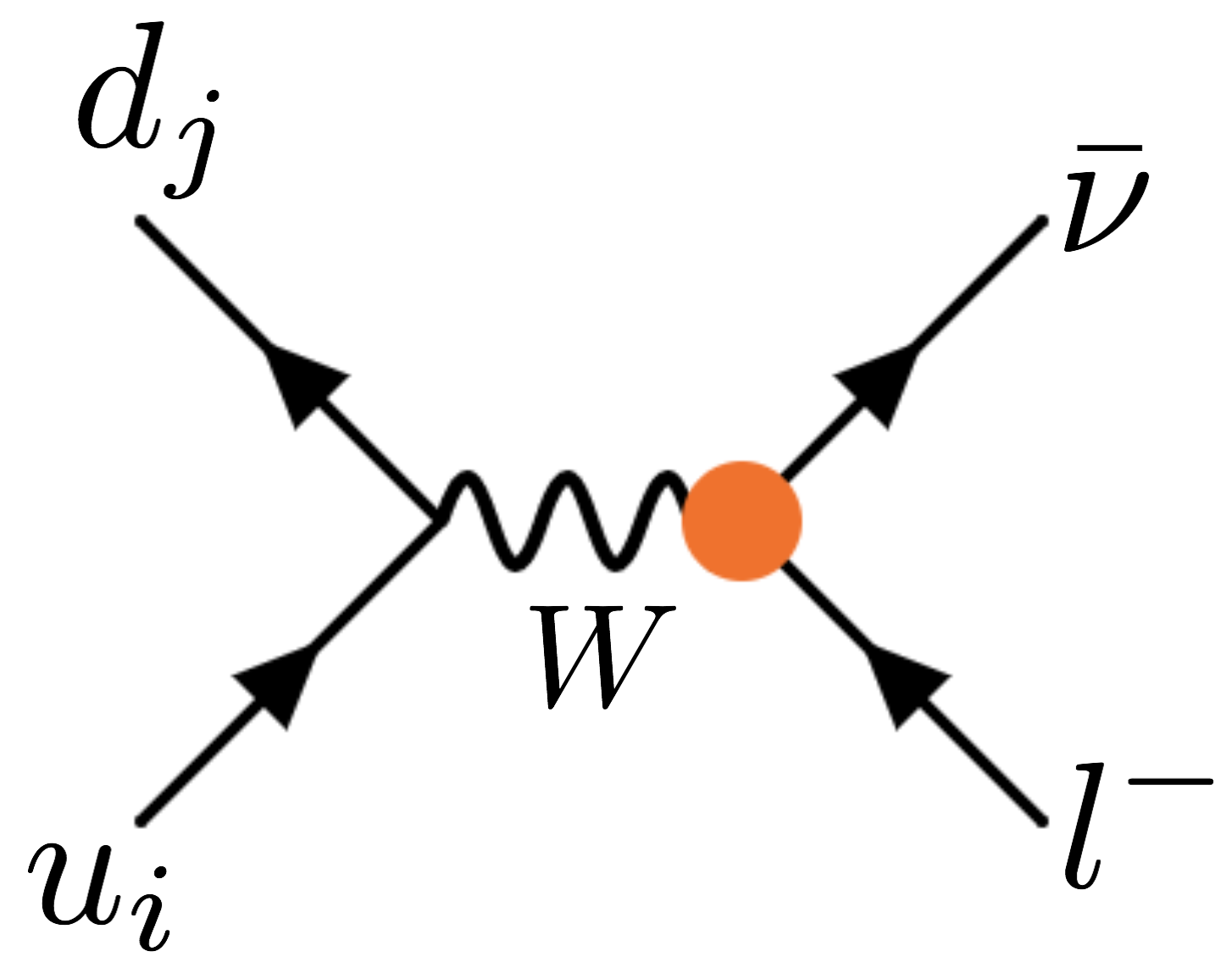
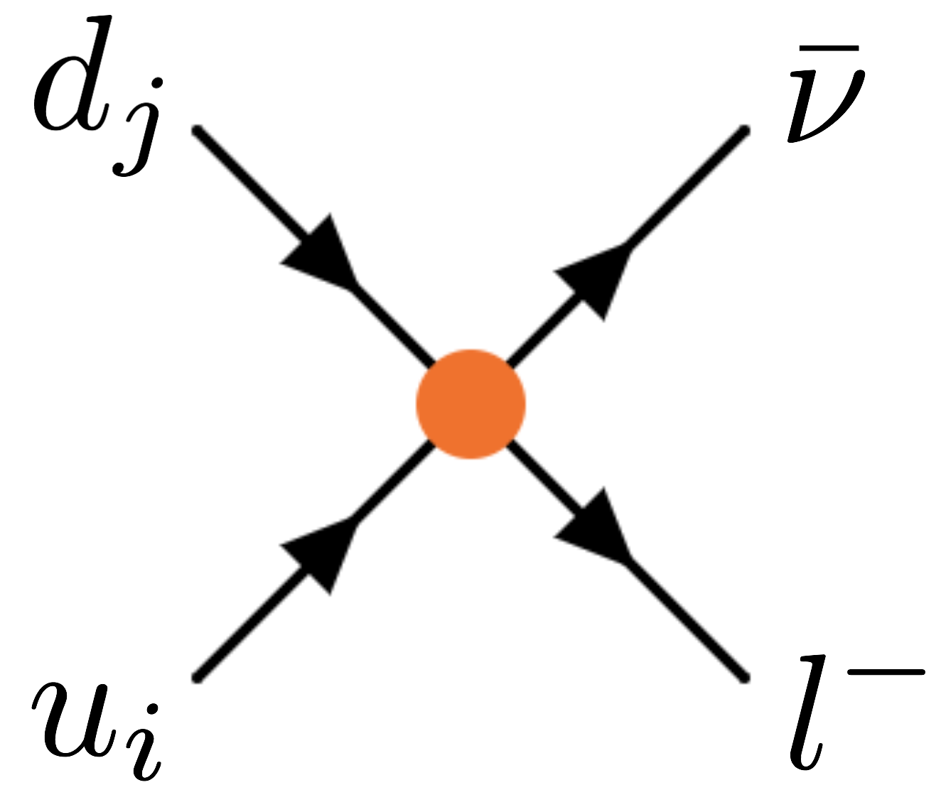
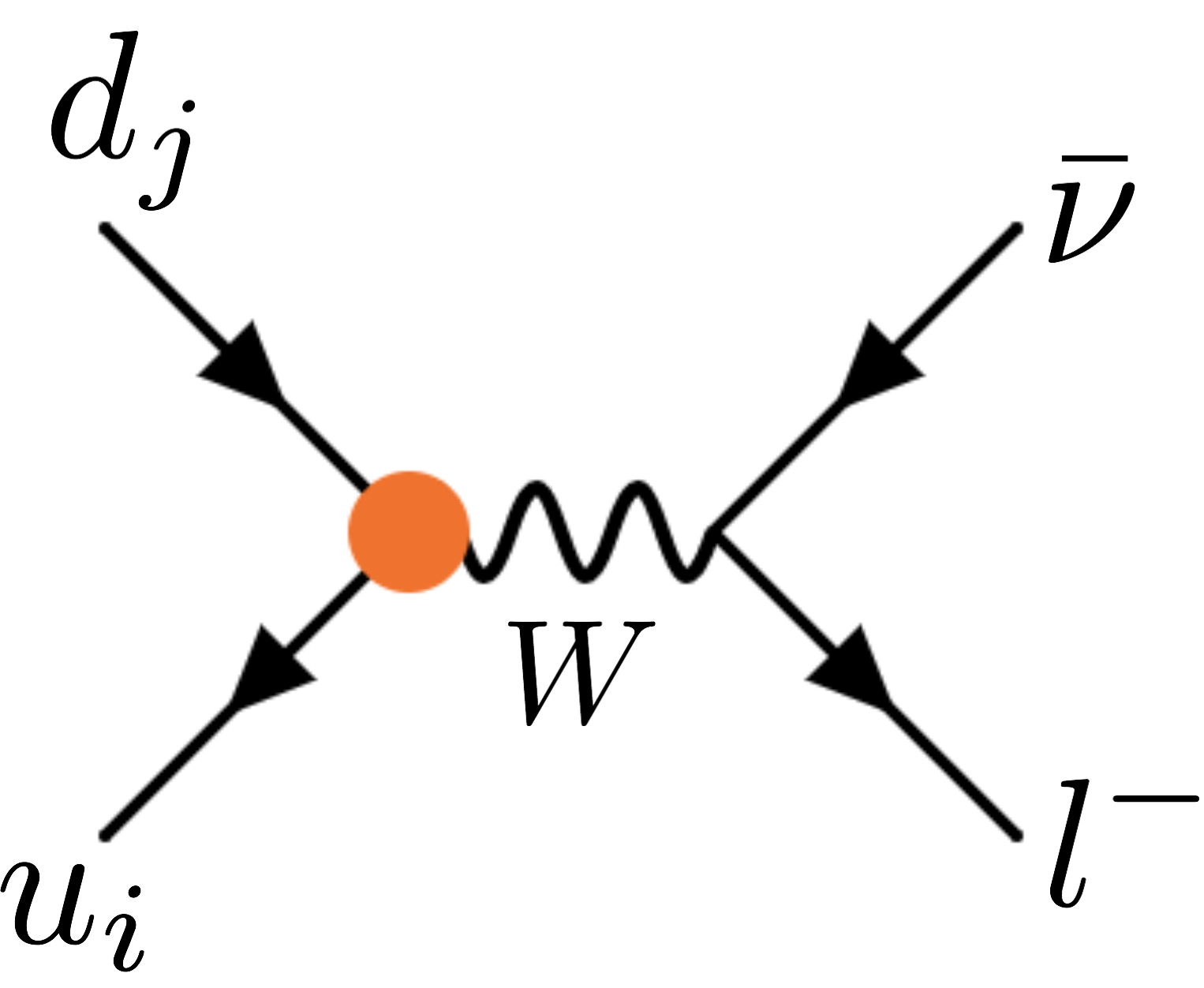
Figure 1: Tree level SMEFT diagrams generating meson decays which also proceed at tree level in the SM. The orange blobs represent insertions of the SMEFT operators Qlq(3)superscriptsubscript𝑄𝑙𝑞3Q_{lq}^{(3)}, QHq(3)superscriptsubscript𝑄𝐻𝑞3Q_{Hq}^{(3)}, and QHl(3)superscriptsubscript𝑄𝐻𝑙3Q_{Hl}^{(3)} respectively.

A starting point for a suitable CKM determination is the Universal Unitarity Triangle (UUT) fit Buras:2000dm ; Blanke:2016bhf . This determination is rooted in the fact that for chosen ratios of FCNC observables, MFV models give predictions that are simply ratios of CKM elements, and the new physics (NP) effects drop out. However, we are prevented from simply applying the UUT here, since it is formulated under the assumption that decays which occur at tree level in the SM (i.e. via a charged-current interaction) are unaffected by NP. In the SMEFT at lowest order in spurions, the NP hierarchy of tree- and loop-induced processes is exactly the same as in the SM; processes which happen at tree-level in the SM are also induced at tree level through a SMEFT operator, while processes which are loop-suppressed in the SM remain loop-suppressed in the SMEFT. To illustrate this point, BSM diagrams which contribute at tree-level to (semi-)leptonic charged-current decays are shown in Fig. 1. All of the operators contributing in Fig. 1 are U(3)5𝑈superscript35U(3)^{5} singlets without Yukawa insertions. We therefore cannot assume that effects in charged-current decays can be neglected, unless these observables are also constructed as ratios in which the NP effects drop out.

Four suitable observables which are unaffected by the leading MFV SMEFT and which we can use to fix the four CKM parameters are

ΔMsΔMd,SψKS,Γ(Kμνμ¯)Γ(πμνμ¯),Γ(BDlν)Γ(Kπlν),Δsubscript𝑀𝑠Δsubscript𝑀𝑑subscript𝑆𝜓subscript𝐾𝑆Γsuperscript𝐾superscript𝜇¯subscript𝜈𝜇Γsuperscript𝜋superscript𝜇¯subscript𝜈𝜇Γ𝐵𝐷𝑙𝜈Γ𝐾𝜋𝑙𝜈\frac{\Delta M_{s}}{\Delta M_{d}},~{}~{}~{}S_{\psi K_{S}},~{}~{}~{}\frac{\Gamma(K^{-}\to\mu^{-}\bar{\nu_{\mu}})}{\Gamma(\pi^{-}\to\mu^{-}\bar{\nu_{\mu}})},~{}~{}~{}\frac{\Gamma(B\to Dl\nu)}{\Gamma(K\to\pi l\nu)}, (12)

where ΔMqΔsubscript𝑀𝑞\Delta M_{q} is the mass difference observable in BqB¯qsubscript𝐵𝑞subscript¯𝐵𝑞B_{q}-\bar{B}_{q} mixing and SψKSsubscript𝑆𝜓subscript𝐾𝑆S_{\psi K_{S}} is the CP asymmetry in B0KSJ/ψsuperscript𝐵0subscript𝐾𝑆𝐽𝜓B^{0}\to K_{S}J/\psi decays. The first two observables are among those that were used in Ref. Blanke:2016bhf to fix the UUT. In App. A, we detail how the effects of NP drop out in these observables, and how they depend on the CKM elements. They constrain, respectively:

|VtdVts|,sin2β,|VusVud|,|VcbVus|,subscript𝑉𝑡𝑑subscript𝑉𝑡𝑠2𝛽subscript𝑉𝑢𝑠subscript𝑉𝑢𝑑subscript𝑉𝑐𝑏subscript𝑉𝑢𝑠\displaystyle\left|\frac{V_{td}}{V_{ts}}\right|,~{}~{}~{}\sin 2\beta,~{}~{}~{}\left|\frac{V_{us}}{V_{ud}}\right|,~{}~{}~{}\left|\frac{V_{cb}}{V_{us}}\right|, (13)

where β𝛽\beta is the CKM angle defined as β=arg[(VcdVcb)/(VtdVtb)]𝛽argdelimited-[]subscript𝑉𝑐𝑑superscriptsubscript𝑉𝑐𝑏subscript𝑉𝑡𝑑superscriptsubscript𝑉𝑡𝑏\beta=\text{arg}\left[-(V_{cd}V_{cb}^{*})/(V_{td}V_{tb}^{*})\right]. From these we fix the four Wolfenstein parameters (see App. A for calculations) to be

(λ=0.2254±0.0005A=0.80±0.013ρ¯=0.187±0.020η¯=0.33±0.05),ρ=(10.080.050.0510.080.0810.961),matrix𝜆absentplus-or-minus0.22540.0005𝐴absentplus-or-minus0.800.013¯𝜌absentplus-or-minus0.1870.020¯𝜂absentplus-or-minus0.330.05𝜌matrix10.080.050.0510.080.0810.961\begin{pmatrix}\lambda=&0.2254\pm 0.0005\\ A=&0.80\pm 0.013\\ \bar{\rho}=&0.187\pm 0.020\\ \bar{\eta}=&0.33\pm 0.05\end{pmatrix},~{}~{}~{}~{}~{}\rho=\begin{pmatrix}1&-0.08&0.05&-0.05\\ \cdot&1&-0.08&-0.08\\ \cdot&\cdot&1&0.96\\ \cdot&\cdot&\cdot&1\end{pmatrix}, (14)

where ρ𝜌\rho is the correlation matrix between the parameters. This determination, being based on just four observables, is unsurprisingly a little less precise than full CKM fits to the SM Charles:2004jd ; Bona:2007vi . Many observables that we will use to constrain the SMEFT do not have dominant CKM errors (instead hadronic or experimental errors dominate), so the constraints will not generally change much at all compared to using the usual SM-fitted CKM to make predictions. In these cases the value of this CKM-determining exercise mostly lies in demonstrating that it is possible to fix the CKM using only observables which are unaffected by NP. However, in some B𝐵B and K𝐾K mixing observables CKM errors can be important, and for these it is necessary to use our CKM values and errors to gain reliable bounds.

3.4 Predictions for flavour observables

Here we detail the flavour observables we consider and how they depend on the WET Wilson coefficients. We calculate constraints from flavour on the WET Wilson coefficients, which may then be used as pseudo-observables in fits to constrain the SMEFT.

The particular structure of the SMEFT under these flavour assumptions means that its effects in flavour observables very closely align with those of the SM itself. This often simplifies things from a calculational point of view, although it can also limit the sensitivity of flavour observables to these NP effects; recall that this is the motivation for adopting an MFV structure in model building. In particular, no contributions are made to operators containing right-handed flavour-changing quark currents, such as 𝒪9=e2(dj¯γμPRdi)(¯γμ)superscriptsubscript𝒪9superscript𝑒2¯subscript𝑑𝑗superscript𝛾𝜇subscript𝑃𝑅subscript𝑑𝑖¯subscript𝛾𝜇\mathcal{O}_{9}^{\prime}=e^{2}\left(\bar{d_{j}}\gamma^{\mu}P_{R}d_{i}\right)\left(\bar{\ell}\gamma_{\mu}\ell\right), which are negligible also in the SM due to the chiral nature of the weak interactions. This in turn ensures that the leading NP effects are linear in the SMEFT coefficients, since there is always an interference term with the SM.

We therefore expect a rather limited number of new constraints arising from the flavour observables considered. The flavour symmetry assumptions ensure that C1,mixbs(xt)subscriptsuperscript𝐶𝑏𝑠1mixsubscript𝑥𝑡C^{bs}_{1,\text{mix}}(x_{t}) and C1,mixsd(xt)subscriptsuperscript𝐶𝑠𝑑1mixsubscript𝑥𝑡C^{sd}_{1,\text{mix}}(x_{t}) depend on the exact same linear combination of SMEFT Wilson coefficients. The same is true for CLbssuperscriptsubscript𝐶𝐿𝑏𝑠C_{L}^{bs} and CLsdsuperscriptsubscript𝐶𝐿𝑠𝑑C_{L}^{sd}. So, anticipating some of the calculations below, we expect to find a maximum of 7 new constrained directions corresponding to constraints on these two coefficients C1,mixdidj(xt)subscriptsuperscript𝐶subscript𝑑𝑖subscript𝑑𝑗1mixsubscript𝑥𝑡C^{d_{i}d_{j}}_{1,\text{mix}}(x_{t}) and CLdidjsuperscriptsubscript𝐶𝐿subscript𝑑𝑖subscript𝑑𝑗C_{L}^{d_{i}d_{j}}, as well as constraints on the three coefficients C7bssuperscriptsubscript𝐶7𝑏𝑠C_{7}^{bs}, C9bssuperscriptsubscript𝐶9𝑏𝑠C_{9}^{bs} and C10bssuperscriptsubscript𝐶10𝑏𝑠C_{10}^{bs} from (semi)leptonic and photonic bs𝑏𝑠b\to s transitions, a constraint on one linear combination of C1bssuperscriptsubscript𝐶1𝑏𝑠C_{1}^{bs} and C2bssuperscriptsubscript𝐶2𝑏𝑠C_{2}^{bs} from the width difference of Bssubscript𝐵𝑠B_{s} mesons, and one constraint from tree-level (semi-)leptonic decays.

3.4.1 Tree level charged-current (semi)leptonic decays

As discussed in the previous section, the leading MFV SMEFT matches at one-loop to operators of the WET that mediate FCNCs. However, there is also one linear combination of SMEFT operators which matches at tree level to the WET operator responsible for charged-current (semi-)leptonic decays via the quark transition diujlν¯subscript𝑑𝑖subscript𝑢𝑗𝑙¯𝜈d_{i}\to u_{j}l\bar{\nu}. This happens through the diagrams in Fig. 1, as well as indirectly through operators entering the measurement of GFsubscript𝐺𝐹G_{F}, which is taken as an electroweak input measurement in both the {αem,mZ,GF}subscript𝛼emsubscript𝑚𝑍subscript𝐺𝐹\left\{\alpha_{\text{em}},m_{Z},G_{F}\right\} and the {mW,mZ,GF}subscript𝑚𝑊subscript𝑚𝑍subscript𝐺𝐹\left\{m_{W},m_{Z},G_{F}\right\} input scheme.

The WET effective Hamiltonian relevant for these charged current decays is

eff=4GFVujdi2C±l(l¯γμPLνl)(u¯iγμPLdj)+h.c..subscripteff4subscript𝐺𝐹subscript𝑉subscript𝑢𝑗subscript𝑑𝑖2subscript𝐶plus-or-minussubscript𝑙¯𝑙subscript𝛾𝜇subscript𝑃𝐿subscript𝜈𝑙subscript¯𝑢𝑖superscript𝛾𝜇subscript𝑃𝐿subscript𝑑𝑗h.c.\displaystyle\mathcal{H}_{\text{eff}}=\frac{4G_{F}V_{u_{j}d_{i}}}{\sqrt{2}}C_{\pm}\sum_{l}\left(\bar{l}\gamma_{\mu}P_{L}\nu_{l}\right)\left(\bar{u}_{i}\gamma^{\mu}P_{L}d_{j}\right)+\text{h.c.}. (15)

The SMEFT contributions to the Wilson coefficient C±subscript𝐶plus-or-minusC_{\pm} are

C±=v2(CHq(3)CHl(3)+Clq(3)+Cll),subscript𝐶plus-or-minussuperscript𝑣2superscriptsubscript𝐶𝐻𝑞3superscriptsubscript𝐶𝐻𝑙3superscriptsubscript𝐶𝑙𝑞3superscriptsubscript𝐶𝑙𝑙C_{\pm}=v^{2}\left(C_{Hq}^{(3)}-C_{Hl}^{(3)}+C_{lq}^{(3)}+C_{ll}^{\prime}\right), (16)

which includes indirect effects due to the fact that GFsubscript𝐺𝐹G_{F} is taken as an input to the theory, and is valid for both electroweak input schemes considered here. Due to the flavour universality of the theory, the same linear combination of SMEFT Wilson coefficients enter into any charged-current decay, so we can constrain it with any well-measured decay. The (radiation-inclusive) SMEFT prediction of Γ(K+μ+νμ)Γsuperscript𝐾superscript𝜇subscript𝜈𝜇\Gamma(K^{+}\to\mu^{+}\nu_{\mu}) is

Γ(K+μ+νμ)=GF28πfK±2mμ2mK±(1mμ2mK±2)2|Vus|2(1+δK)(1+2C±),Γsuperscript𝐾superscript𝜇subscript𝜈𝜇superscriptsubscript𝐺𝐹28𝜋superscriptsubscript𝑓superscript𝐾plus-or-minus2superscriptsubscript𝑚𝜇2subscript𝑚superscript𝐾plus-or-minussuperscript1superscriptsubscript𝑚𝜇2superscriptsubscript𝑚superscript𝐾plus-or-minus22superscriptsubscript𝑉𝑢𝑠21subscript𝛿𝐾12subscript𝐶plus-or-minus\displaystyle\Gamma(K^{+}\to\mu^{+}\nu_{\mu})=\frac{G_{F}^{2}}{8\pi}f_{K^{\pm}}^{2}m_{\mu}^{2}m_{K^{\pm}}\left(1-\frac{m_{\mu}^{2}}{m_{K^{\pm}}^{2}}\right)^{2}\left|V_{us}\right|^{2}\left(1+\delta_{K}\right)\left(1+2C_{\pm}\right), (17)

where fK±=155.7(0.3)subscript𝑓superscript𝐾plus-or-minus155.70.3f_{K^{\pm}}=155.7(0.3) MeV is the charged kaon decay constant Aoki:2019cca , and δK=0.0107(21)subscript𝛿𝐾0.010721\delta_{K}=0.0107(21) is a radiative correction factor Tanabashi:2018oca . This leads (using our CKM inputs) to a SM prediction of Γ(K+μ+νμ)SM=(3.381±0.020)×108Γsubscriptsuperscript𝐾superscript𝜇subscript𝜈𝜇SMplus-or-minus3.3810.020superscript108\Gamma(K^{+}\to\mu^{+}\nu_{\mu})_{\text{SM}}=(3.381\pm 0.020)\times 10^{-8} eV, while the experimental value is Γ(K+μ+νμ)exp=3.3793(79)×108Γsubscriptsuperscript𝐾superscript𝜇subscript𝜈𝜇exp3.379379superscript108\Gamma(K^{+}\to\mu^{+}\nu_{\mu})_{\text{exp}}=3.3793(79)\times 10^{-8} eV. Then the bound on C±subscript𝐶plus-or-minusC_{\pm} is

C±=0.000±0.003.subscript𝐶plus-or-minusplus-or-minus0.0000.003C_{\pm}=0.000\pm 0.003. (18)

3.4.2 Bs,dsubscript𝐵𝑠𝑑B_{s,d} mixing observables ΔMs,dΔsubscript𝑀𝑠𝑑\Delta M_{s,d} and ΔΓs,dΔsubscriptΓ𝑠𝑑\Delta\Gamma_{s,d}

One observable that can be measured in Bs,dsubscript𝐵𝑠𝑑B_{s,d} mixing is the mass difference of the two neutral mass eigenstates, ΔMs,dΔsubscript𝑀𝑠𝑑\Delta M_{s,d}. In our case where C1,mixsubscript𝐶1mixC_{1,\text{mix}} is the only non-zero ΔB=2Δ𝐵2\Delta B=2 operator coefficient, the theoretical expression for the SM+NP mass difference for Bs,dsubscript𝐵𝑠𝑑B_{s,d} mixing, normalised to the SM, is simply DiLuzio:2019jyq

ΔMs,dSM+NPΔMs,dSM=|1+C1,mixb(s,d)(xt)S0(xt)|,Δsuperscriptsubscript𝑀𝑠𝑑SM+NPΔsuperscriptsubscript𝑀𝑠𝑑SM1subscriptsuperscript𝐶𝑏𝑠𝑑1mixsubscript𝑥𝑡subscript𝑆0subscript𝑥𝑡\frac{\Delta M_{s,d}^{\text{SM+NP}}}{\Delta M_{s,d}^{\text{SM}}}=\left|1+\frac{C^{b(s,d)}_{1,\text{mix}}(x_{t})}{S_{0}(x_{t})}\right|, (19)

since the hadronic matrix elements and QCD corrections are identical for the SM and NP parts. The function S0(xt)subscript𝑆0subscript𝑥𝑡S_{0}(x_{t}) is the usual Inami-Lim function Inami:1980fz , given by

S0(xt)=4xt11xt2+xt34(1xt)23xt32(1xt)3logxt2.31.subscript𝑆0subscript𝑥𝑡4subscript𝑥𝑡11superscriptsubscript𝑥𝑡2superscriptsubscript𝑥𝑡34superscript1subscript𝑥𝑡23superscriptsubscript𝑥𝑡32superscript1subscript𝑥𝑡3subscript𝑥𝑡2.31S_{0}(x_{t})=\frac{4x_{t}-11x_{t}^{2}+x_{t}^{3}}{4(1-x_{t})^{2}}-\frac{3x_{t}^{3}}{2(1-x_{t})^{3}}\log x_{t}\approx 2.31. (20)

The measured values are Amhis:2016xyh

ΔMdexpΔsuperscriptsubscript𝑀𝑑exp\displaystyle\Delta M_{d}^{\text{exp}} =(0.5064±0.0019)ps1,absentplus-or-minus0.50640.0019superscriptps1\displaystyle=\left(0.5064\pm 0.0019\right)\text{ps}^{-1}, (21)
ΔMsexpΔsuperscriptsubscript𝑀𝑠exp\displaystyle\Delta M_{s}^{\text{exp}} =(17.757±0.021)ps1.absentplus-or-minus17.7570.021superscriptps1\displaystyle=\left(17.757\pm 0.021\right)\text{ps}^{-1}. (22)

To be consistent with the CKM input scheme (see Sec. 3.3), we are only able to use one of these as a constraint on the SMEFT, since we used the ratio as an input to fix the CKM parameters; we choose ΔMsΔsubscript𝑀𝑠\Delta M_{s} because of its slightly more precise measurement. We furthermore need to calculate the SM prediction using the derived CKM parameters in Eqn. (14), and the associated error. This will be important in this case because the CKM is already a significant source of error for state-of-the-art SM predictions of ΔMqΔsubscript𝑀𝑞\Delta M_{q}, and our CKM determination, being based on fewer measurements, has larger errors than traditional fits. The SM prediction is

ΔMsSM=GF2mW2mBs6π2S0(xt)η2B|VtsVtb|2fBs2B^Bq(1),Δsuperscriptsubscript𝑀𝑠SMsuperscriptsubscript𝐺𝐹2superscriptsubscript𝑚𝑊2subscript𝑚subscript𝐵𝑠6superscript𝜋2subscript𝑆0subscript𝑥𝑡subscript𝜂2𝐵superscriptsuperscriptsubscript𝑉𝑡𝑠subscript𝑉𝑡𝑏2superscriptsubscript𝑓subscript𝐵𝑠2superscriptsubscript^𝐵subscript𝐵𝑞1\Delta M_{s}^{\text{SM}}=\frac{G_{F}^{2}m_{W}^{2}m_{B_{s}}}{6\pi^{2}}S_{0}(x_{t})\eta_{2B}\left|V_{ts}^{*}V_{tb}\right|^{2}f_{B_{s}}^{2}\hat{B}_{B_{q}}^{(1)}, (23)

where fBsB^Bq(1)subscript𝑓subscript𝐵𝑠superscriptsubscript^𝐵subscript𝐵𝑞1f_{B_{s}}\sqrt{\hat{B}_{B_{q}}^{(1)}} can be calculated on the lattice (we use the results of Ref. Dowdall:2019bea ) and η2Bsubscript𝜂2𝐵\eta_{2B} is a QCD correction factor, given at NLO in Ref. Buras:1990fn . We obtain the prediction

ΔMsSM=(17.2±1.1)ps1,Δsuperscriptsubscript𝑀𝑠SMplus-or-minus17.21.1superscriptps1\Delta M_{s}^{\text{SM}}=(17.2\pm 1.1)\,\text{ps}^{-1}, (24)

leading to a bound on the WET Wilson coefficient of

C1,mixbs(xt)superscriptsubscript𝐶1mix𝑏𝑠subscript𝑥𝑡\displaystyle C_{1,\text{mix}}^{bs}(x_{t}) =0.070.15+0.17.absentsubscriptsuperscript0.070.170.15\displaystyle=0.07^{+0.17}_{-0.15}. (25)

The decay rate difference of Bssubscript𝐵𝑠B_{s} mesons, ΔΓsΔsubscriptΓ𝑠\Delta\Gamma_{s}, is sensitive to new bc¯cs𝑏¯𝑐𝑐𝑠b\to\bar{c}cs effects, and is thus dependent on the coefficients C1bssuperscriptsubscript𝐶1𝑏𝑠C_{1}^{bs} and C2bssuperscriptsubscript𝐶2𝑏𝑠C_{2}^{bs} of the Hamiltonian in Eqn. (7). The observable is defined as ΔΓs=2|Γ12s,SM+Γ12s,NP|cosϕ12sΔsubscriptΓ𝑠2superscriptsubscriptΓ12𝑠SMsuperscriptsubscriptΓ12𝑠NPsubscriptsuperscriptitalic-ϕ𝑠12\Delta\Gamma_{s}=2|\Gamma_{12}^{s,\text{SM}}+\Gamma_{12}^{s,\text{NP}}|\cos\phi^{s}_{12}, where cosϕ12s1subscriptsuperscriptitalic-ϕ𝑠121\cos\phi^{s}_{12}\approx 1, and Jager:2017gal

Γ12s,NPsuperscriptsubscriptΓ12𝑠NP\displaystyle\Gamma_{12}^{s,\text{NP}} =GF2λc2mb2MBsfBs21zc36π×\displaystyle=-G_{F}^{2}\lambda_{c}^{2}m_{b}^{2}M_{Bs}f_{Bs}^{2}\frac{\sqrt{1-z_{c}}}{36\pi}\times
[(8(1zc/4)C2SMC2NP+4(1zc)(3C1SMC1NP+C1SMC2NP+C2SMC1NP))B\displaystyle\bigg{[}\Big{(}8(1-z_{c}/4)\,C_{2}^{\text{SM}}C_{2}^{\text{NP}}+4(1-z_{c})\left(3C_{1}^{\text{SM}}C_{1}^{\text{NP}}+C_{1}^{\text{SM}}C_{2}^{\text{NP}}+C_{2}^{\text{SM}}C_{1}^{\text{NP}}\right)\Big{)}B
+(1+zc/2)(C2SMC2NPC1SMC2NPC2SMC1NP+3C1SMC1NP)B~S],\displaystyle+(1+z_{c}/2)(C_{2}^{\text{SM}}C_{2}^{\text{NP}}-C_{1}^{\text{SM}}C_{2}^{\text{NP}}-C_{2}^{\text{SM}}C_{1}^{\text{NP}}+3C_{1}^{\text{SM}}C_{1}^{\text{NP}})\,\tilde{B}_{S}^{\prime}\,\bigg{]}, (26)

where zc=4mc2/mb2subscript𝑧𝑐4superscriptsubscript𝑚𝑐2superscriptsubscript𝑚𝑏2z_{c}=4m_{c}^{2}/m_{b}^{2}, λc=VcsVcbsubscript𝜆𝑐superscriptsubscript𝑉𝑐𝑠subscript𝑉𝑐𝑏\lambda_{c}=V_{cs}^{*}V_{cb}, fBssubscript𝑓𝐵𝑠f_{Bs} is the Bssubscript𝐵𝑠B_{s} decay constant, B𝐵B and B~Ssuperscriptsubscript~𝐵𝑆\tilde{B}_{S}^{\prime} are bag parameters, and C1,2SMsuperscriptsubscript𝐶12SMC_{1,2}^{\text{SM}} and C1,2NPsuperscriptsubscript𝐶12NPC_{1,2}^{\text{NP}} are the SM and NP contributions respectively to C1,2bs(μb)superscriptsubscript𝐶12𝑏𝑠subscript𝜇𝑏C_{1,2}^{bs}(\mu_{b}). The SM coefficients are C1SM(μb)=0.2451superscriptsubscript𝐶1SMsubscript𝜇𝑏0.2451C_{1}^{\text{SM}}(\mu_{b})=-0.2451, C2SM(μb)=1.008superscriptsubscript𝐶2SMsubscript𝜇𝑏1.008C_{2}^{\text{SM}}(\mu_{b})=1.008 at NNLO in QCD Gorbahn:2004my . For the values of hadronic parameters we refer to Jager:2019bgk and references therein. The measured value is Amhis:2016xyh

ΔΓsexpΔsuperscriptsubscriptΓ𝑠exp\displaystyle\Delta\Gamma_{s}^{\text{exp}} =(0.088±0.006)ps1.absentplus-or-minus0.0880.006superscriptps1\displaystyle=(0.088\pm 0.006)\,\text{ps}^{-1}. (27)

while the SM prediction is Artuso:2015swg 666This prediction assumes values and errors for the CKM elements from the 2014 web update of the CKMfitter group Charles:2004jd . To be fully consistent, we should recalculate it using our CKM inputs. However, the large error on this prediction is dominated by the uncertainty on hadronic bag parameters, form factors and renormalisation scale dependence Amhis:2016xyh . Using our CKM inputs would shift the central value by a tiny amount compared to the total error, and our larger error on Vcbsubscript𝑉𝑐𝑏V_{cb} (which represents the dominant CKM uncertainty in this prediction) has the result of inflating the total error from 22.7%percent22.722.7\% to 24.4%percent24.424.4\%. We perform our fits using this slightly larger error, but the effects of this are imperceptible.

ΔΓsSMΔsuperscriptsubscriptΓ𝑠SM\displaystyle\Delta\Gamma_{s}^{\text{SM}} =(0.088±0.020)ps1.absentplus-or-minus0.0880.020superscriptps1\displaystyle=(0.088\pm 0.020)\,\text{ps}^{-1}. (28)

From the above, (adding experimental and theoretical errors in quadrature), we obtain a constraint at 1σ𝜎\sigma on a linear combination of the NP WET Wilson coefficients:

|C2bs(μb)+0.01C1bs(μb)|<0.09,superscriptsubscript𝐶2𝑏𝑠subscript𝜇𝑏0.01superscriptsubscript𝐶1𝑏𝑠subscript𝜇𝑏0.09\displaystyle\left|C_{2}^{bs}(\mu_{b})+0.01C_{1}^{bs}(\mu_{b})\right|<0.09, (29)

where Jager:2017gal

(C1bs(μb)C2bs(μb))matrixsuperscriptsubscript𝐶1𝑏𝑠subscript𝜇𝑏superscriptsubscript𝐶2𝑏𝑠subscript𝜇𝑏\displaystyle\begin{pmatrix}C_{1}^{bs}(\mu_{b})\\ C_{2}^{bs}(\mu_{b})\end{pmatrix} =(1.120.270.271.12)(C1bs(mW)C2bs(mW)).absentmatrix1.120.270.271.12matrixsuperscriptsubscript𝐶1𝑏𝑠subscript𝑚𝑊superscriptsubscript𝐶2𝑏𝑠subscript𝑚𝑊\displaystyle=\begin{pmatrix}1.12&-0.27\\ -0.27&1.12\end{pmatrix}\begin{pmatrix}C_{1}^{bs}(m_{W})\\ C_{2}^{bs}(m_{W})\end{pmatrix}. (30)

The percentage error on the measurement of ΔΓdΔsubscriptΓ𝑑\Delta\Gamma_{d}, the decay rate difference of Bdsubscript𝐵𝑑B_{d} mesons, is much larger than that on ΔΓsΔsubscriptΓ𝑠\Delta\Gamma_{s} Amhis:2016xyh . This observable is dependent on the exact same linear combination of leading MFV SMEFT coefficients as ΔΓsΔsubscriptΓ𝑠\Delta\Gamma_{s}, and would produce much weaker bounds, so we don’t include it in our analysis.

3.4.3 εKsubscript𝜀𝐾\varepsilon_{K}

The observable εKsubscript𝜀𝐾\varepsilon_{K} determines indirect CP violation in kaon mixing, and is defined:

εK=κεeiϕε2(ΔMK)expImM12,subscript𝜀𝐾subscript𝜅𝜀superscript𝑒𝑖subscriptitalic-ϕ𝜀2subscriptΔsubscript𝑀𝐾expImsubscript𝑀12\displaystyle\varepsilon_{K}=\frac{\kappa_{\varepsilon}e^{i\phi_{\varepsilon}}}{\sqrt{2}\left(\Delta M_{K}\right)_{\text{exp}}}\,\text{Im}M_{12}, (31)

where κε=0.94±0.02subscript𝜅𝜀plus-or-minus0.940.02\kappa_{\varepsilon}=0.94\pm 0.02 Buras:2010pza , ϕε=(43.52±0.05)subscriptitalic-ϕ𝜀plus-or-minus43.520.05\phi_{\varepsilon}=(43.52\pm 0.05) Tanabashi:2018oca , ΔMKMKLMKS=(3.484±0.006)×1012Δsubscript𝑀𝐾subscript𝑀subscript𝐾𝐿subscript𝑀subscript𝐾𝑆plus-or-minus3.4840.006superscript1012\Delta M_{K}\equiv M_{K_{L}}-M_{K_{S}}=(3.484\pm 0.006)\times 10^{-12} MeV Tanabashi:2018oca . The prediction for |εK|subscript𝜀𝐾|\varepsilon_{K}| in the MFV SMEFT is hence (λi=VisVidsubscript𝜆𝑖subscriptsuperscript𝑉𝑖𝑠subscript𝑉𝑖𝑑\lambda_{i}=V^{*}_{is}V_{id})

|εK|subscript𝜀𝐾\displaystyle\left|\varepsilon_{K}\right| =κεCεB^KImλt(Reλc[η1(C1,mixsd(xc)+S0(xc))η3(C1,mixsd(xc,xt)+S0(xc,xt))]\displaystyle=\kappa_{\varepsilon}C_{\varepsilon}\hat{B}_{K}\text{Im}\lambda_{t}\bigg{(}\text{Re}\lambda_{c}\left[\eta_{1}(C^{sd}_{1,\text{mix}}(x_{c})+S_{0}(x_{c}))-\eta_{3}(C^{sd}_{1,\text{mix}}(x_{c},x_{t})+S_{0}(x_{c},x_{t}))\right]
Reλtη2(C1,mixsd(xt)+S0(xt))),\displaystyle-\text{Re}\lambda_{t}\eta_{2}(C^{sd}_{1,\text{mix}}(x_{t})+S_{0}(x_{t}))\bigg{)}, (32)

where the C1,mixsdsubscriptsuperscript𝐶𝑠𝑑1mixC^{sd}_{1,\text{mix}} coefficients are the NP Wilson coefficients of the effective Hamiltonian in Eqn. (3.1). The S0subscript𝑆0S_{0} coefficients are the SM contributions, which are given by the Inami-Lim functions Inami:1980fz (with xk=mk2/mW2subscript𝑥𝑘superscriptsubscript𝑚𝑘2superscriptsubscript𝑚𝑊2x_{k}=m_{k}^{2}/m_{W}^{2}):

S0(xt)subscript𝑆0subscript𝑥𝑡\displaystyle S_{0}(x_{t}) =4xt11xt2+xt34(1xt)23xt32(1xt)3logxt,absent4subscript𝑥𝑡11superscriptsubscript𝑥𝑡2superscriptsubscript𝑥𝑡34superscript1subscript𝑥𝑡23superscriptsubscript𝑥𝑡32superscript1subscript𝑥𝑡3subscript𝑥𝑡\displaystyle=\frac{4x_{t}-11x_{t}^{2}+x_{t}^{3}}{4(1-x_{t})^{2}}-\frac{3x_{t}^{3}}{2(1-x_{t})^{3}}\log x_{t}, (33)
S0(xc)subscript𝑆0subscript𝑥𝑐\displaystyle S_{0}(x_{c}) =xc,absentsubscript𝑥𝑐\displaystyle=x_{c}, (34)
S0(xt,xc)subscript𝑆0subscript𝑥𝑡subscript𝑥𝑐\displaystyle S_{0}(x_{t},x_{c}) =xc(logxtxc3xt4(1xt)3xt24(1xt)2logxt).absentsubscript𝑥𝑐subscript𝑥𝑡subscript𝑥𝑐3subscript𝑥𝑡41subscript𝑥𝑡3superscriptsubscript𝑥𝑡24superscript1subscript𝑥𝑡2subscript𝑥𝑡\displaystyle=x_{c}\left(\log\frac{x_{t}}{x_{c}}-\frac{3x_{t}}{4(1-x_{t})}-\frac{3x_{t}^{2}}{4(1-x_{t})^{2}}\log x_{t}\right). (35)

The short distance QCD factors are given at NLO Buchalla:1995vs by η1=1.38subscript𝜂11.38\eta_{1}=1.38, η2=0.574subscript𝜂20.574\eta_{2}=0.574 and η3=0.47subscript𝜂30.47\eta_{3}=0.47. The parameter B^Ksubscript^𝐵𝐾\hat{B}_{K} is proportional to the hadronic matrix element and can be calculated on the lattice; a recent average finds B^K=0.7625±0.0097subscript^𝐵𝐾plus-or-minus0.76250.0097\hat{B}_{K}=0.7625\pm 0.0097 Aoki:2019cca . Finally, the overall factor Cεsubscript𝐶𝜀C_{\varepsilon} is given by

Cε=GF2fK2mK0mW262π2(ΔMK)exp.subscript𝐶𝜀superscriptsubscript𝐺𝐹2superscriptsubscript𝑓𝐾2subscript𝑚superscript𝐾0superscriptsubscript𝑚𝑊262superscript𝜋2subscriptΔsubscript𝑀𝐾exp\displaystyle C_{\varepsilon}=\frac{G_{F}^{2}f_{K}^{2}m_{K^{0}}m_{W}^{2}}{6\sqrt{2}\pi^{2}\left(\Delta M_{K}\right)_{\text{exp}}}. (36)

Using the CKM values and errors of Sec 3.3, the SM prediction is

|εK|SM=(1.8±0.3)×103,subscriptsubscript𝜀𝐾SMplus-or-minus1.80.3superscript103\left|\varepsilon_{K}\right|_{\text{SM}}=(1.8\pm 0.3)\times 10^{-3}, (37)

while the measured value is

|εK|exp=(2.228±0.011)×103.subscriptsubscript𝜀𝐾expplus-or-minus2.2280.011superscript103\left|\varepsilon_{K}\right|_{\text{exp}}=(2.228\pm 0.011)\times 10^{-3}. (38)

This leads, via Eqn. (32), to a constraint on the linear combination of C1,mixsdsubscriptsuperscript𝐶𝑠𝑑1mixC^{sd}_{1,\text{mix}} coefficients (assuming that the total NP part is smaller than the SM contribution):

0.95C1,mixsd(xc)+0.32C1,mixsd(xt,xc)+5.8×10⁴C1,mixsd(xt)=(0.40±0.30)×103.0.95subscriptsuperscript𝐶𝑠𝑑1mixsubscript𝑥𝑐0.32subscriptsuperscript𝐶𝑠𝑑1mixsubscript𝑥𝑡subscript𝑥𝑐5.8superscript104subscriptsuperscript𝐶𝑠𝑑1mixsubscript𝑥𝑡plus-or-minus0.400.30superscript103-0.95\,C^{sd}_{1,\text{mix}}(x_{c})+0.32\,C^{sd}_{1,\text{mix}}(x_{t},x_{c})+5.8\times 10^{-4}\,C^{sd}_{1,\text{mix}}(x_{t})=(0.40\pm 0.30)\times 10^{-3}. (39)

3.4.4 Kπν¯ν𝐾𝜋¯𝜈𝜈K\to\pi\bar{\nu}\nu

For NP in which the neutrinos are coupled to left-handed currents only (which is the case for the leading MFV SMEFT), the expressions for the branching ratios are Buras:2015yca ; Buras:2015qea

(K+π+ν¯ν)superscript𝐾superscript𝜋¯𝜈𝜈\displaystyle\mathcal{B}\left(K^{+}\to\pi^{+}\bar{\nu}\nu\right) =κ+(1+ΔEM)[(ImXeffλ5)2+(ReλcλPc(X)+ReXeffλ5)2],absentsubscript𝜅1subscriptΔEMdelimited-[]superscriptImsubscript𝑋effsuperscript𝜆52superscriptResubscript𝜆𝑐𝜆subscript𝑃𝑐𝑋Resubscript𝑋effsuperscript𝜆52\displaystyle=\kappa_{+}\left(1+\Delta_{\text{EM}}\right)\left[\left(\frac{\text{Im}\,X_{\text{eff}}}{\lambda^{5}}\right)^{2}+\left(\frac{\text{Re}\,\lambda_{c}}{\lambda}\,P_{c}(X)+\frac{\text{Re}\,X_{\text{eff}}}{\lambda^{5}}\right)^{2}\right], (40)
(KLπ0ν¯ν)subscript𝐾𝐿superscript𝜋0¯𝜈𝜈\displaystyle\mathcal{B}\left(K_{L}\to\pi^{0}\bar{\nu}\nu\right) =κL(ImXeffλ5)2,absentsubscript𝜅𝐿superscriptImsubscript𝑋effsuperscript𝜆52\displaystyle=\kappa_{L}\left(\frac{\text{Im}\,X_{\text{eff}}}{\lambda^{5}}\right)^{2}, (41)

where

κ+subscript𝜅\displaystyle\kappa_{+} =(5.173±0.025)×1011[λ0.225]8,absentplus-or-minus5.1730.025superscript1011superscriptdelimited-[]𝜆0.2258\displaystyle=(5.173\pm 0.025)\times 10^{-11}\left[\frac{\lambda}{0.225}\right]^{8}, ΔEM=0.003,subscriptΔEM0.003\displaystyle\Delta_{\text{EM}}=-0.003, (42)
κLsubscript𝜅𝐿\displaystyle\kappa_{L} =(2.231±0.013)×1010[λ0.225]8.absentplus-or-minus2.2310.013superscript1010superscriptdelimited-[]𝜆0.2258\displaystyle=(2.231\pm 0.013)\times 10^{-10}\left[\frac{\lambda}{0.225}\right]^{8}. (43)

Here λ=|Vus|𝜆subscript𝑉𝑢𝑠\lambda=|V_{us}|, λi=VisVidsubscript𝜆𝑖subscriptsuperscript𝑉𝑖𝑠subscript𝑉𝑖𝑑\lambda_{i}=V^{*}_{is}V_{id}, ΔEMsubscriptΔEM\Delta_{\text{EM}} is the radiative electromagnetic correction, and κ+subscript𝜅\kappa_{+} and κLsubscript𝜅𝐿\kappa_{L} summarise the remaining factors, including the hadronic matrix elements. The loop functions for the top and charm quark contributions, Xeffsubscript𝑋effX_{\text{eff}} and Pc(X)subscript𝑃𝑐𝑋P_{c}(X), are given in the SM by Buras:2015qea

Pc(X)subscript𝑃𝑐𝑋\displaystyle P_{c}(X) =0.404±0.024,absentplus-or-minus0.4040.024\displaystyle=0.404\pm 0.024, (44)
XeffSMsuperscriptsubscript𝑋effSM\displaystyle X_{\text{eff}}^{\text{SM}} =VtsVtdXLSM,absentsuperscriptsubscript𝑉𝑡𝑠subscript𝑉𝑡𝑑superscriptsubscript𝑋𝐿SM\displaystyle=V_{ts}^{*}V_{td}\,X_{L}^{\text{SM}}, XLSM=1.481±0.009.superscriptsubscript𝑋𝐿SMplus-or-minus1.4810.009\displaystyle X_{L}^{\text{SM}}=1.481\pm 0.009. (45)

In the presence of the SMEFT contributions,777neglecting the suppressed effect of NP in the charm loops Xeffsubscript𝑋effX_{\text{eff}} becomes

XeffSM+NP=VtsVtd(XLSMCLsd(μK)),superscriptsubscript𝑋effSM+NPsuperscriptsubscript𝑉𝑡𝑠subscript𝑉𝑡𝑑superscriptsubscript𝑋𝐿SMsuperscriptsubscript𝐶𝐿𝑠𝑑subscript𝜇𝐾X_{\text{eff}}^{\text{SM+NP}}=V_{ts}^{*}V_{td}\left(X_{L}^{\text{SM}}-C_{L}^{sd}(\mu_{K})\right), (46)

with μK=2subscript𝜇𝐾2\mu_{K}=2 GeV. For the experimental limits, we take the recent upper bound from NA62 NA62:2019

(K+π+ν¯ν)superscript𝐾superscript𝜋¯𝜈𝜈\displaystyle\mathcal{B}\left(K^{+}\to\pi^{+}\bar{\nu}\nu\right) <1.85×10¹⁰(90% CL),absent1.85superscript101090% CL\displaystyle<1.85\times 10^{-10}\,~{}(\text{90\% CL}), (47)

and from the 2015 run at KOTO Ahn:2018mvc

(KLπ0ν¯ν)subscript𝐾𝐿superscript𝜋0¯𝜈𝜈\displaystyle\mathcal{B}\left(K_{L}\to\pi^{0}\bar{\nu}\nu\right) <3.0×10⁹(90% CL).absent3.0superscript10990% CL\displaystyle<3.0\times 10^{-9}\,~{}(\text{90\% CL}). (48)

These lead to a bound on the NP contribution to the WET Wilson coefficient:

CLsd(μK)superscriptsubscript𝐶𝐿𝑠𝑑subscript𝜇𝐾\displaystyle C_{L}^{sd}(\mu_{K}) =2.1±2.8.absentplus-or-minus2.12.8\displaystyle=2.1\pm 2.8. (49)

This coefficient barely runs, so we can take CLsd(μK)CLsd(mW)superscriptsubscript𝐶𝐿𝑠𝑑subscript𝜇𝐾superscriptsubscript𝐶𝐿𝑠𝑑subscript𝑚𝑊C_{L}^{sd}(\mu_{K})\approx C_{L}^{sd}(m_{W}).

3.4.5 BK()ν¯ν𝐵superscript𝐾¯𝜈𝜈B\to K^{(*)}\bar{\nu}\nu

Following Ref. Buras:2014fpa , the predictions for the branching ratios in the presence of the MFV SMEFT contributions can be written (in our notation)

(BK()ν¯ν)SM+NP(BK()ν¯ν)SM=|CLbs(mb)XtSM|XtSM,subscript𝐵superscript𝐾¯𝜈𝜈SM+NPsubscript𝐵superscript𝐾¯𝜈𝜈SMsuperscriptsubscript𝐶𝐿𝑏𝑠subscript𝑚𝑏superscriptsubscript𝑋𝑡SMsuperscriptsubscript𝑋𝑡SM\displaystyle\frac{\mathcal{B}\left(B\to K^{(*)}\bar{\nu}\nu\right)_{\text{SM+NP}}}{\mathcal{B}\left(B\to K^{(*)}\bar{\nu}\nu\right)_{\text{SM}}}=\frac{\left|C_{L}^{bs}(m_{b})-X_{t}^{\text{SM}}\right|}{X_{t}^{\text{SM}}}, (50)

where

XtSM=1.469±0.017.superscriptsubscript𝑋𝑡SMplus-or-minus1.4690.017X_{t}^{\text{SM}}=1.469\pm 0.017. (51)

The experimental limits on the branching ratios, measured at BaBar Lees:2013kla and Belle Lutz:2013ftz are

(B+K+ν¯ν)superscript𝐵superscript𝐾¯𝜈𝜈\displaystyle\mathcal{B}\left(B^{+}\to K^{+}\bar{\nu}\nu\right) <1.7×10⁵(90% CL),absent1.7superscript10590% CL\displaystyle<1.7\times 10^{-5}\,~{}(\text{90\% CL}), (52)
(B0K0ν¯ν)superscript𝐵0superscript𝐾absent0¯𝜈𝜈\displaystyle\mathcal{B}\left(B^{0}\to K^{*0}\bar{\nu}\nu\right) <5.5×10⁵(90% CL),absent5.5superscript10590% CL\displaystyle<5.5\times 10^{-5}\,~{}(\text{90\% CL}), (53)

which lead to bounds on the ratios, at 90% CL, of Buras:2014fpa

(B+K+ν¯ν)SM+NP(B+K+ν¯ν)SM<4.3,subscriptsuperscript𝐵superscript𝐾¯𝜈𝜈SM+NPsubscriptsuperscript𝐵superscript𝐾¯𝜈𝜈SM4.3\displaystyle\frac{\mathcal{B}\left(B^{+}\to K^{+}\bar{\nu}\nu\right)_{\text{SM+NP}}}{\mathcal{B}\left(B^{+}\to K^{+}\bar{\nu}\nu\right)_{\text{SM}}}<4.3, (54)
(B0K0ν¯ν)SM+NP(B+K+ν¯ν)SM<4.4.subscriptsuperscript𝐵0superscript𝐾absent0¯𝜈𝜈SM+NPsubscriptsuperscript𝐵superscript𝐾¯𝜈𝜈SM4.4\displaystyle\frac{\mathcal{B}\left(B^{0}\to K^{*0}\bar{\nu}\nu\right)_{\text{SM+NP}}}{\mathcal{B}\left(B^{+}\to K^{+}\bar{\nu}\nu\right)_{\text{SM}}}<4.4. (55)

These lead to a bound on the NP part of the WET Wilson coefficient:

CLbs(μb)superscriptsubscript𝐶𝐿𝑏𝑠subscript𝜇𝑏\displaystyle C_{L}^{bs}(\mu_{b}) =1.5±3.9.absentplus-or-minus1.53.9\displaystyle=1.5\pm 3.9. (56)

As above, we can take CLbs(μb)CLbs(mW)superscriptsubscript𝐶𝐿𝑏𝑠subscript𝜇𝑏superscriptsubscript𝐶𝐿𝑏𝑠subscript𝑚𝑊C_{L}^{bs}(\mu_{b})\approx C_{L}^{bs}(m_{W}) since the running is very small.

3.4.6 bsγ𝑏𝑠𝛾b\to s\gamma and bsl+l𝑏𝑠superscript𝑙superscript𝑙b\to sl^{+}l^{-} processes

Processes involving the parton level transitions bsγ𝑏𝑠𝛾b\to s\gamma and bsl+l𝑏𝑠superscript𝑙superscript𝑙b\to sl^{+}l^{-}, for example branching ratios and angular observables of BK()l+l𝐵superscript𝐾superscript𝑙superscript𝑙B\to K^{(*)}l^{+}l^{-}, and branching ratios of BXsγ𝐵subscript𝑋𝑠𝛾B\to X_{s}\gamma and Bsl+lsubscript𝐵𝑠superscript𝑙superscript𝑙B_{s}\to l^{+}l^{-}, can constrain the WET Wilson coefficients C7bssuperscriptsubscript𝐶7𝑏𝑠C_{7}^{bs}, C9bssuperscriptsubscript𝐶9𝑏𝑠C_{9}^{bs} and C10bssuperscriptsubscript𝐶10𝑏𝑠C_{10}^{bs}.888The bd𝑏𝑑b\to d WET coefficients C7bdsuperscriptsubscript𝐶7𝑏𝑑C_{7}^{bd}, C9bdsuperscriptsubscript𝐶9𝑏𝑑C_{9}^{bd} and C10bdsuperscriptsubscript𝐶10𝑏𝑑C_{10}^{bd} depend on the same linear combinations of SMEFT Wilson coefficients under our flavour assumptions as these bs𝑏𝑠b\to s ones. Currently, new physics in the theoretically clean bdl+l𝑏𝑑superscript𝑙superscript𝑙b\to dl^{+}l^{-} and bdγ𝑏𝑑𝛾b\to d\gamma processes is not well constrained, but this should change in the future with measurements of inclusive bd𝑏𝑑b\to d processes at Belle II Crivellin:2011ba ; Huber:2019iqf . We use flavio Straub:2018kue to find the vector 𝑪^bold-^𝑪\bm{\hat{C}} of best fit values of the Wilson coefficients, and to numerically extract the variances and correlation matrix by expanding Δχ2Δsuperscript𝜒2\Delta\chi^{2} around the best fit point as

Δχ2=(𝑪𝑪^)TU1(𝑪𝑪^),Δsuperscript𝜒2superscript𝑪bold-^𝑪𝑇superscript𝑈1𝑪bold-^𝑪\displaystyle\Delta\chi^{2}=\left(\bm{C}-\bm{\hat{C}}\right)^{T}U^{-1}\left(\bm{C}-\bm{\hat{C}}\right), (57)

where the covariance matrix U𝑈U can be written in terms of the variances σi2superscriptsubscript𝜎𝑖2\sigma_{i}^{2} and the correlation matrix ρ𝜌\rho as Uij=σiσjρijsubscript𝑈𝑖𝑗subscript𝜎𝑖subscript𝜎𝑗subscript𝜌𝑖𝑗U_{ij}=\sigma_{i}\sigma_{j}\rho_{ij} (no sum). In this way we find constraints on the new physics Wilson coefficients of

(C7bs(μb)C9bs(μb)C10bs(μb))matrixsuperscriptsubscript𝐶7𝑏𝑠subscript𝜇𝑏superscriptsubscript𝐶9𝑏𝑠subscript𝜇𝑏superscriptsubscript𝐶10𝑏𝑠subscript𝜇𝑏\displaystyle\begin{pmatrix}C_{7}^{bs}(\mu_{b})\\ C_{9}^{bs}(\mu_{b})\\ C_{10}^{bs}(\mu_{b})\\ \end{pmatrix} =(0.002±0.0150.40±0.300.40±0.19)absentmatrixplus-or-minus0.0020.015plus-or-minus0.400.30plus-or-minus0.400.19\displaystyle=\begin{pmatrix}-0.002\pm 0.015\\ -0.40\pm 0.30\\ 0.40\pm 0.19\end{pmatrix} (58)

with the correlation matrix

ρ=(1.000.230.010.231.000.430.010.431.00).𝜌matrix1.000.230.010.231.000.430.010.431.00\displaystyle\rho=\begin{pmatrix}1.00~{}&-0.23~{}&0.01\\ -0.23~{}&1.00~{}&0.43\\ 0.01~{}&0.43~{}&1.00\end{pmatrix}. (59)

The observables that are included in this flavio fit are based on the list of rare B𝐵B decay observables involving a bs𝑏𝑠b\to s transition given in Ref. Aebischer:2018iyb (and we refer to this reference as well as Ref. Straub:2018kue for the measurements and theory predictions that are included in the flavio code). Specifically, the observables used are: all relevant CP-averaged observables in semileptonic bsμμ𝑏𝑠𝜇𝜇b\to s\mu\mu decays that were included in the global fit of Ref. Altmannshofer:2017fio (except for angular observables in BKμμ𝐵superscript𝐾𝜇𝜇B\to K^{*}\mu\mu), high-q2superscript𝑞2q^{2} branching ratios and angular observables of ΛbΛμμsubscriptΛ𝑏Λ𝜇𝜇\Lambda_{b}\to\Lambda\mu\mu, the branching ratios of B0μμsuperscript𝐵0𝜇𝜇B^{0}\to\mu\mu and Bsμμsubscript𝐵𝑠𝜇𝜇B_{s}\to\mu\mu, the branching ratio of the inclusive decay BXsμμ𝐵subscript𝑋𝑠𝜇𝜇B\to X_{s}\mu\mu, and all observables in inclusive and exclusive radiative bsγ𝑏𝑠𝛾b\to s\gamma decays included in the fit of Ref. Paul:2016urs , including BKee𝐵superscript𝐾𝑒𝑒B\to K^{*}ee at low q2superscript𝑞2q^{2}. We do not fit to observables that test lepton flavour universality, or lepton flavour violation, since under our flavour assumptions these will not be altered from their SM predictions. We also exclude angular observables in the decay BKμμ𝐵superscript𝐾𝜇𝜇B\to K^{*}\mu\mu from the fit, due to the presence of as-yet unknown power corrections in the theory predictions which could mimic some effects of BSM physics Jager:2012uw ; Jager:2014rwa ; Descotes-Genon:2014uoa ; Ciuchini:2015qxb ; Capdevila:2017bsm ; Chobanova:2017ghn ; Bobeth:2017vxj ; Arbey:2018ics ; Chrzaszcz:2018yza ; Hurth:2020rzx . If a real estimate of these power corrections were established and found not to be too large, including these observables in the fit would have the effect of shrinking the errors on the Wilson coefficients slightly, and moving the central value of C9bs(μb)superscriptsubscript𝐶9𝑏𝑠subscript𝜇𝑏C_{9}^{bs}(\mu_{b}) further from zero.

The constrained Wilson coefficients at μbsubscript𝜇𝑏\mu_{b}=4.2 GeV are related to the Wilson coefficients at mWsubscript𝑚𝑊m_{W} by Aebischer:2018bkb :

C7bs(μb)superscriptsubscript𝐶7𝑏𝑠subscript𝜇𝑏\displaystyle C_{7}^{bs}(\mu_{b}) =0.65C7bs(mW)+9.6102C8bs(mW),absent0.65superscriptsubscript𝐶7𝑏𝑠subscript𝑚𝑊9.6superscript102superscriptsubscript𝐶8𝑏𝑠subscript𝑚𝑊\displaystyle=0.65\,C_{7}^{bs}(m_{W})+9.6\cdot 10^{-2}\,C_{8}^{bs}(m_{W}),
C9bs(μb)superscriptsubscript𝐶9𝑏𝑠subscript𝜇𝑏\displaystyle C_{9}^{bs}(\mu_{b}) =8.46C1bs(mW)+2.04C2bs(mW)+0.98C9bs(mW),absent8.46superscriptsubscript𝐶1𝑏𝑠subscript𝑚𝑊2.04superscriptsubscript𝐶2𝑏𝑠subscript𝑚𝑊0.98superscriptsubscript𝐶9𝑏𝑠subscript𝑚𝑊\displaystyle=8.46\,C_{1}^{bs}(m_{W})+2.04\,C_{2}^{bs}(m_{W})+0.98\,C_{9}^{bs}(m_{W}),
C10bs(μb)superscriptsubscript𝐶10𝑏𝑠subscript𝜇𝑏\displaystyle C_{10}^{bs}(\mu_{b}) =1.0C10bs(mW).absent1.0superscriptsubscript𝐶10𝑏𝑠subscript𝑚𝑊\displaystyle=1.0\,C_{10}^{bs}(m_{W}). (60)

4 Fit

We perform an illustrative fit, within the {αem,mZ,GF}subscript𝛼𝑒𝑚subscript𝑚𝑍subscript𝐺𝐹\{\alpha_{em},m_{Z},G_{F}\} input scheme, to demonstrate the effect that flavour observables have within a global fit assuming flavour symmetry. We assume Gaussian errors throughout and fit using the method of least squares. We include all operators allowed by our flavour and CP assumptions.

4.1 Observables and data

Our choice of non-flavour observables is motivated by the following considerations, with the aim of getting a fair picture of the new physical information that flavour can add to a global fit: (a) we want to include observables which provide strong and up-to-date constraints on operators involving EW gauge bosons and Higgs fields, and (b) we want to include observables which depend on the same 4-fermion operators that appear at one-loop in FCNCs. With this in mind, we include the following:

  • Precision electroweak observables: We use the LEPI observables and predictions from Table 2 of Ref. Brivio:2017bnu , as well as the W𝑊W mass Tanabashi:2018oca and the forward-backward asymmetries AFB0,fsuperscriptsubscript𝐴𝐹𝐵0𝑓A_{FB}^{0,f} for f={c,b,}𝑓𝑐𝑏f=\{c,b,\ell\}. The measurements and their correlations come from Ref. ALEPH:2005ab .

  • LEPII W+Wsuperscript𝑊superscript𝑊W^{+}W^{-}: We use all the data and SM predictions (Achard:2004zw ; Abbiendi:2007rs ; Heister:2004wr ; Schael:2013ita ) from Tables 12, 13, 14 and 15 of Ref. Berthier:2016tkq , and the definitions of the observables in terms of SMEFT parameters from Tables 2 and 3 of the same reference.

  • Higgs Run I: We use the combined ATLAS and CMS Run I Higgs signal strength measurements from Table 8 of Ref. Khachatryan:2016vau , with the correlation matrix in Figure 27 of the same reference. For the SMEFT predictions we adopt the definitions of the observables in terms of Warsaw-basis Wilson coefficients provided in the Mathematica notebook accompanying Ref. Ellis:2018gqa .

  • Higgs Run II: From the CMS paper Sirunyan:2018koj , we use all the signal strength measurements in Table 3, and the correlation matrix from the supplementary material. From the ATLAS paper Aad:2019mbh we use all the cross sections times branching ratios in Table 6 and the correlation matrix in Figure 6. For the SMEFT predictions we use the definitions of the observables in terms of Warsaw basis Wilson coefficients provided in the Mathematica notebook accompanying Ref. Ellis:2018gqa .

  • W+Wsuperscript𝑊superscript𝑊W^{+}W^{-} production at LHC: Following Ref. Ellis:2018gqa , we use a measurement of one bin of the differential cross section of ppW+We±νμ±ν𝑝𝑝superscript𝑊superscript𝑊superscript𝑒plus-or-minus𝜈superscript𝜇plus-or-minus𝜈pp\to W^{+}W^{-}\to e^{\pm}\nu\mu^{\pm}\nu at ATLAS Aaboud:2017qkn , using the definitions of the observable in terms of SMEFT Wilson coefficients provided in the Mathematica notebook accompanying Ref. Ellis:2018gqa .

  • e+eq¯qsuperscript𝑒superscript𝑒¯𝑞𝑞e^{+}e^{-}\to\bar{q}q off the Z𝑍Z pole: We use the data on σhadsubscript𝜎𝑎𝑑\sigma_{had} at different values of s𝑠\sqrt{s} from Table 6 of Ref. Berthier:2015gja . The original experimental results are from LEP Schael:2013ita and TRIDENT TRISTAN:1994 and the SM predictions are taken from Ref. Arbuzov:2005ma .

  • Low energy precision measurements: From the Appendix of Ref. Berthier:2015gja , we use observables and data on Atomic Parity Violation Vetter:1995vf ; Wood:1997zq and eDIS Prescott:1979dh . From Ref. Falkowski:2017pss , we use observables and data on neutrino-nucleon scattering (both νesubscript𝜈𝑒\nu_{e} scattering data from CHARM Allaby:1987vr and νμsubscript𝜈𝜇\nu_{\mu} scattering data from the PDG average Tanabashi:2018oca ), deep inelastic scattering of polarized electrons Tanabashi:2018oca ; Beise:2004py , and deep inelastic scattering of muons Argento:1982tq .

  • Flavour observables: We use the constraints on WET Wilson coefficients given in Section 3.4.

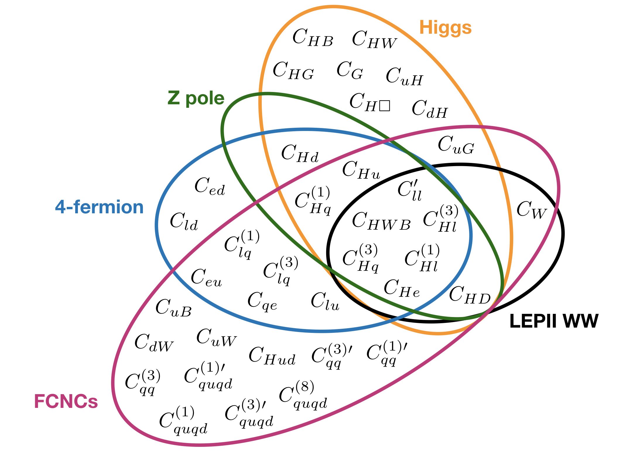
This is a total of 187 observables. Figure 2 shows which Wilson coefficients in the Warsaw basis affect each set of observables, where the “4-fermion” category includes low energy precision measurements as well as e+eq¯qsuperscript𝑒superscript𝑒¯𝑞𝑞e^{+}e^{-}\to\bar{q}q off the Z𝑍Z pole.

Refer to caption
Figure 2: Diagram showing which Warsaw basis Wilson coefficients affect each of the types of observables included in the fit

4.2 Fit methodology

The SMEFT corrections to all the observables are linear in the dimension 6 Wilson coefficients (under our flavour and CP assumptions and working to O(Λ2)𝑂superscriptΛ2O(\Lambda^{-2})), meaning that predictions for the observables can be written as a matrix equation

𝝁(𝜽)=𝝁SM+𝐇𝜽,𝝁𝜽subscript𝝁𝑆𝑀𝐇𝜽\bm{\mu}\left(\bm{\theta}\right)=\bm{\mu}_{SM}+\mathbf{H}\cdot\bm{\theta}, (61)

where 𝝁𝝁\bm{\mu} is the vector of predictions, 𝝁SMsubscript𝝁𝑆𝑀\bm{\mu}_{SM} represents the SM predictions, 𝜽𝜽\bm{\theta} is a vector of SMEFT Wilson coefficients, and 𝐇𝐇\mathbf{H} is a matrix of functions that parameterise the SMEFT corrections. The measured central values of the observables can be represented by a vector 𝐲𝐲\mathbf{y}, with a covariance matrix 𝐕𝐕\mathbf{V}. Then the χ2superscript𝜒2\chi^{2} function is

χ2(𝜽)=(𝐲𝝁(𝜽))T𝐕1(𝐲𝝁(𝜽)).superscript𝜒2𝜽superscript𝐲𝝁𝜽𝑇superscript𝐕1𝐲𝝁𝜽\chi^{2}(\bm{\theta})=\left(\mathbf{y}-\bm{\mu}\left(\bm{\theta}\right)\right)^{T}\mathbf{V}^{-1}\left(\mathbf{y}-\bm{\mu}\left(\bm{\theta}\right)\right). (62)

The least-squares estimators 𝜽^bold-^𝜽\bm{\hat{\theta}} for the Wilson coefficients are found by minimising χ2superscript𝜒2\chi^{2}:

𝜽^=(𝐇T𝐕1𝐇)1𝐇T𝐕1𝐲.bold-^𝜽superscriptsuperscript𝐇𝑇superscript𝐕1𝐇1superscript𝐇𝑇superscript𝐕1𝐲\bm{\hat{\theta}}=\left(\mathbf{H}^{T}\mathbf{V}^{-1}\mathbf{H}\right)^{-1}\mathbf{H}^{T}\mathbf{V}^{-1}\mathbf{y}. (63)

The covariance matrix 𝐔𝐔\mathbf{U} for the least squares estimators is given by the inverse of the Fisher matrix 𝐅𝐅\mathbf{F}, defined as

𝐅=𝐇T𝐕1𝐇=𝐔1.𝐅superscript𝐇𝑇superscript𝐕1𝐇superscript𝐔1\mathbf{F}=\mathbf{H}^{T}\mathbf{V}^{-1}\mathbf{H}=\mathbf{U}^{-1}. (64)

When the covariance matrix is diagonalised, its entries are the variances σi2superscriptsubscript𝜎𝑖2\sigma_{i}^{2} of its eigenvectors, which are a set of linearly independent directions in Wilson coefficient space. The eigenvalues of the Fisher matrix are therefore 1/σi21superscriptsubscript𝜎𝑖21/\sigma_{i}^{2}. If an eigenvector direction is unconstrained by the data, its corresponding Fisher matrix eigenvalue will be zero.

4.3 Flavour in the electroweak hyperplane

If we (artificially, but for purposes of illustration) restrict attention to the set of ten Wilson coefficients that enter the Z𝑍Z-pole observables,

{CHWB,CHD,CHl(1),CHl(3),CHq(1),CHq(3),CHu,CHd,CHe,Cll},subscript𝐶𝐻𝑊𝐵subscript𝐶𝐻𝐷superscriptsubscript𝐶𝐻𝑙1superscriptsubscript𝐶𝐻𝑙3superscriptsubscript𝐶𝐻𝑞1superscriptsubscript𝐶𝐻𝑞3subscript𝐶𝐻𝑢subscript𝐶𝐻𝑑subscript𝐶𝐻𝑒superscriptsubscript𝐶𝑙𝑙\{C_{HWB},C_{HD},C_{Hl}^{(1)},C_{Hl}^{(3)},C_{Hq}^{(1)},C_{Hq}^{(3)},C_{Hu},C_{Hd},C_{He},C_{ll}^{\prime}\}, (65)

then it is well-known that fitting only to Z𝑍Z-pole observables leaves two flat directions. We define these as999These are linear combinations of the flat directions given in Ref. Brivio:2017bnu . This reference also provides an explanation of why these occur, in terms of a reparameterization invariance of 22222\to 2 fermion scattering processes in the SMEFT.

k1=0.369(\displaystyle k_{1}=0.369\bigg{(} 13CHd2CHD+CHe+12CHl(1)16CHq(1)23CHu5.12(CHq(3)+CHl(3))13subscript𝐶𝐻𝑑2subscript𝐶𝐻𝐷subscript𝐶𝐻𝑒12superscriptsubscript𝐶𝐻𝑙116superscriptsubscript𝐶𝐻𝑞123subscript𝐶𝐻𝑢5.12superscriptsubscript𝐶𝐻𝑞3superscriptsubscript𝐶𝐻𝑙3\displaystyle\frac{1}{3}C_{Hd}-2C_{HD}+C_{He}+\frac{1}{2}C_{Hl}^{(1)}-\frac{1}{6}C_{Hq}^{(1)}-\frac{2}{3}C_{Hu}-5.12(C_{Hq}^{(3)}+C_{Hl}^{(3)})
+3.62CHWB),\displaystyle+3.62C_{HWB}\bigg{)}, (66)
k2=0.118(\displaystyle k_{2}=-0.118\bigg{(} 13CHd2CHD+CHe+12CHl(1)16CHq(1)23CHu+0.77(CHq(3)+CHl(3))13subscript𝐶𝐻𝑑2subscript𝐶𝐻𝐷subscript𝐶𝐻𝑒12superscriptsubscript𝐶𝐻𝑙116superscriptsubscript𝐶𝐻𝑞123subscript𝐶𝐻𝑢0.77superscriptsubscript𝐶𝐻𝑞3superscriptsubscript𝐶𝐻𝑙3\displaystyle\frac{1}{3}C_{Hd}-2C_{HD}+C_{He}+\frac{1}{2}C_{Hl}^{(1)}-\frac{1}{6}C_{Hq}^{(1)}-\frac{2}{3}C_{Hu}+0.77(C_{Hq}^{(3)}+C_{Hl}^{(3)})
+0.56CHWB).\displaystyle+0.56C_{HWB}\bigg{)}. (67)

These flat directions must be closed by other, often less well-measured, observables. In Figure 3 we show, within the plane of the Wilson coefficients of these two flat directions, the constraints from the flavour observables (in green), which can be compared to those obtained from LEP II WW𝑊𝑊WW production (in orange) and LHC Higgs measurements (in blue). In all cases the Z𝑍Z-pole data are also included in the fit. The axes correspond to the k1subscript𝑘1k_{1} and k2subscript𝑘2k_{2} directions, which have been normalised to unit vectors in Wilson coefficient space. We define the norm |k|𝑘|k| of an operator direction by assuming an arbitrary Euclidean metric δijsubscript𝛿𝑖𝑗\delta_{ij} in the Warsaw basis; if we write k=𝒄𝜽𝑘𝒄𝜽k=\bm{c}\cdot\bm{\theta}, where as before 𝜽𝜽\bm{\theta} is the vector of Warsaw basis Wilson coefficients, then |k|2δijcicjsuperscript𝑘2subscript𝛿𝑖𝑗subscript𝑐𝑖subscript𝑐𝑗|k|^{2}\equiv\delta_{ij}\,c_{i}c_{j}. All of the ellipses in Figure 3 are obtained by taking only this set of 10 Wilson coefficients (65) to be non-zero, and profiling over the 8 linearly independent directions (which are already well constrained by the Z𝑍Z-pole data). Under these assumptions, it can be seen that flavour is competitive with existing constraints within this highly flavourless plane.
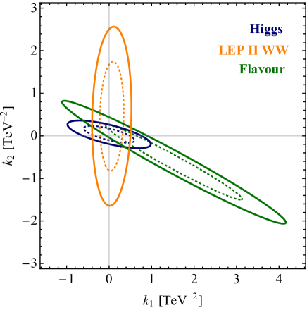
Refer to caption
Figure 3: Flavour (green), Higgs (blue) and LEP II WW𝑊𝑊WW (orange) constraints on the plane of the Z𝑍Z-pole flat directions, under the assumptions explained in the text. The dotted lines are 1σ1𝜎1\sigma contours, the solid lines are 2σ2𝜎2\sigma contours. The axes correspond to the coefficients of the two independent linear combinations of Wilson coefficients that remain unconstrained by the Z𝑍Z-pole data, as defined in sections 4.3 and 67.

4.4 Eigensystem of the global fit

While the limited fit presented in the previous subsection gives an indication of the power of current flavour measurements when compared like-for-like with Higgs and LEP II WW𝑊𝑊WW measurements, a more global picture — without artificially setting coefficients to zero — is needed for a realistic interpretation of the constraints. The observables we include in the fit, within our flavour assumption, depend on a total of 37 Wilson coefficients in the Warsaw basis:

{CH,CHWB,CHD,CHW,CHB,CHG,CW,CG,CHl(1),CHl(3),CHq(1),CHq(3),CHu,CHd,CHe,\displaystyle\{C_{H\Box},C_{HWB},C_{HD},C_{HW},C_{HB},C_{HG},C_{W},C_{G},C_{Hl}^{(1)},C_{Hl}^{(3)},C_{Hq}^{(1)},C_{Hq}^{(3)},C_{Hu},C_{Hd},C_{He},
CHud,CuH,CdH,CuW,CdW,CuB,CuG,Cll,Clq(3),Clq(1),Cqe,Clu,Cld,Ceu,Ced,subscript𝐶𝐻𝑢𝑑subscript𝐶𝑢𝐻subscript𝐶𝑑𝐻subscript𝐶𝑢𝑊subscript𝐶𝑑𝑊subscript𝐶𝑢𝐵subscript𝐶𝑢𝐺superscriptsubscript𝐶𝑙𝑙subscriptsuperscript𝐶3𝑙𝑞subscriptsuperscript𝐶1𝑙𝑞subscript𝐶𝑞𝑒subscript𝐶𝑙𝑢subscript𝐶𝑙𝑑subscript𝐶𝑒𝑢subscript𝐶𝑒𝑑\displaystyle C_{Hud},C_{uH},C_{dH},C_{uW},C_{dW},C_{uB},C_{uG},C_{ll}^{\prime},C^{(3)}_{lq},C^{(1)}_{lq},C_{qe},C_{lu},C_{ld},C_{eu},C_{ed},
Cqq(1),Cqq(3),Cqq(3),Cquqd(1),Cquqd(8),Cquqd(1),Cquqd(8)}.\displaystyle C^{(1)\prime}_{qq},C^{(3)}_{qq},C^{(3)\prime}_{qq},C^{(1)}_{quqd},C^{(8)}_{quqd},C^{(1)\prime}_{quqd},C^{(8)\prime}_{quqd}\}. (68)

Including all observables above, we have 7 flat directions (corresponding to the null space of the Fisher matrix):

(f1,f2,f3,f4,f5,\displaystyle(f_{1},f_{2},f_{3},f_{4},f_{5}, f6,f7)T=\displaystyle f_{6},f_{7})^{T}= (69)
𝔸(Cqq(1)+Cqq(3),Cquqd(1),Cquqd(1),Cquqd(8),Cquqd(8),CdW,CG,CHud,CuG,CuH)T𝔸superscriptsuperscriptsubscript𝐶𝑞𝑞1superscriptsubscript𝐶𝑞𝑞3superscriptsubscript𝐶𝑞𝑢𝑞𝑑1superscriptsubscript𝐶𝑞𝑢𝑞𝑑1superscriptsubscript𝐶𝑞𝑢𝑞𝑑8superscriptsubscript𝐶𝑞𝑢𝑞𝑑8subscript𝐶𝑑𝑊subscript𝐶𝐺subscript𝐶𝐻𝑢𝑑subscript𝐶𝑢𝐺subscript𝐶𝑢𝐻𝑇\displaystyle\mathbb{A}(C_{qq}^{(1)\prime}+C_{qq}^{(3)\prime},C_{quqd}^{(1)},C_{quqd}^{(1)\prime},C_{quqd}^{(8)},C_{quqd}^{(8)\prime},C_{dW},C_{G},C_{Hud},C_{uG},C_{uH})^{T}

where the matrix 𝔸𝔸\mathbb{A} is given by

𝔸=(0.240.490.240.600.350.000.230.000.070.220.200.510.610.110.400.150.210.000.060.210.510.260.340.060.470.010.200.000.060.190.070.360.080.530.680.040.230.050.070.220.360.520.650.120.120.040.090.040.030.080.090.160.090.560.160.080.540.030.170.530.020.010.030.060.030.040.001.000.000.00)𝔸matrix0.240.490.240.600.350.000.230.000.070.220.200.510.610.110.400.150.210.000.060.210.510.260.340.060.470.010.200.000.060.190.070.360.080.530.680.040.230.050.070.220.360.520.650.120.120.040.090.040.030.080.090.160.090.560.160.080.540.030.170.530.020.010.030.060.030.040.001.000.000.00\displaystyle\mathbb{A}=\begin{pmatrix}-0.24&-0.49&-0.24&0.60&0.35&0.00&0.23&0.00&0.07&-0.22\\ 0.20&-0.51&-0.61&-0.11&-0.40&0.15&-0.21&0.00&-0.06&0.21\\ 0.51&0.26&-0.34&0.06&0.47&-0.01&0.20&0.00&0.06&-0.19\\ 0.07&0.36&-0.08&0.53&-0.68&-0.04&0.23&-0.05&0.07&-0.22\\ 0.36&-0.52&0.65&0.12&-0.12&-0.04&0.09&-0.04&0.03&-0.08\\ 0.09&0.16&0.09&0.56&0.16&-0.08&-0.54&-0.03&-0.17&0.53\\ 0.02&0.01&0.03&0.06&-0.03&0.04&0.00&1.00&0.00&0.00\end{pmatrix} (70)

If the flavour observables are excluded from the fit, there are 12 flat directions — the flavour data adds 5 new constraints.

The set of simultaneous constraints that can be extracted from the fit can be illustrated by the eigenvalues of the Fisher matrix, 1/σi21superscriptsubscript𝜎𝑖21/\sigma_{i}^{2}, defined in Section 4.2. The values of σisubscript𝜎𝑖\sigma_{i} can be taken as bounds on the coefficients cisubscript𝑐𝑖c_{i} of the respective eigenvector directions, or equivalently σi1/2superscriptsubscript𝜎𝑖12\sigma_{i}^{-1/2} provides a lower bound on the scale of suppression of the eigenvector operator (1/|ci|>σi1/21subscript𝑐𝑖superscriptsubscript𝜎𝑖121/\sqrt{|c_{i}|}>\sigma_{i}^{-1/2}), remembering that the cisubscript𝑐𝑖c_{i}s have dimension TeV-2. In this way, the effect of adding flavour data to the fit is demonstrated in Figure 4. The addition of flavour data changes the eigenvector directions, and therefore not all the eigenvalues can be directly compared. With this in mind, we have plotted the eigenvalues of the full fit in size order, pairing each with the eigenvalue of the fit without flavour whose corresponding eigenvector (𝒆Fsuperscript𝒆cancel𝐹\bm{e}^{\cancel{F}}) has the largest overlap with the relevant eigenvector of the full fit (𝒆Fsuperscript𝒆𝐹\bm{e}^{F}), where this overlap is defined as

δij𝒆iF𝒆jF|𝒆F||𝒆F|.subscript𝛿𝑖𝑗subscriptsuperscript𝒆cancel𝐹𝑖subscriptsuperscript𝒆𝐹𝑗superscript𝒆cancel𝐹superscript𝒆𝐹\frac{\delta_{ij}\,\bm{e}^{\cancel{F}}_{i}\bm{e}^{F}_{j}}{|\bm{e}^{\cancel{F}}||\bm{e}^{F}|}. (71)

For the well-constrained eigenvectors (towards the left of the plot), the overlap is close to 1. The five otherwise flat directions which are closed by flavour data can be seen in the plot as blue bars without an accompanying green bar (four of these are at order TeV or above). In particular, two directions which are unconstrained without flavour data are now paired to rather well-constrained directions in the full fit (1/|c9|>5.71subscript𝑐95.71/\sqrt{|c_{9}|}>5.7 TeV and 1/|c11|>4.81subscript𝑐114.81/\sqrt{|c_{11}|}>4.8 TeV respectively). These directions (eigenvectors of the full fit) are dependent on nearly all the Wilson coefficients in Eqn. (4.4), but can be written approximately as

𝒆9Fsuperscriptsubscript𝒆9𝐹\displaystyle\bm{e}_{9}^{F} 0.58(Cqq(1)Cqq(3))+0.29Cqq(3)+0.19CdW+0.22CHe+0.22CHl(1)absent0.58superscriptsubscript𝐶𝑞𝑞1superscriptsubscript𝐶𝑞𝑞30.29superscriptsubscript𝐶𝑞𝑞30.19subscript𝐶𝑑𝑊0.22subscript𝐶𝐻𝑒0.22superscriptsubscript𝐶𝐻𝑙1\displaystyle\approx 0.58\left(C_{qq}^{(1)\prime}-C_{qq}^{(3)\prime}\right)+0.29C_{qq}^{(3)}+0.19C_{dW}+0.22C_{He}+0.22C_{Hl}^{(1)}
+0.17CHWB+0.15CHD0.12Clq(1)+,0.17subscript𝐶𝐻𝑊𝐵0.15subscript𝐶𝐻𝐷0.12superscriptsubscript𝐶𝑙𝑞1\displaystyle+0.17C_{HWB}+0.15C_{HD}-0.12C_{lq}^{(1)}+\ldots, (72)
𝒆11Fsuperscriptsubscript𝒆11𝐹\displaystyle\bm{e}_{11}^{F} 0.85CdW+0.27CuB0.20CuW0.18(Cqq(1)Cqq(3))+0.12Cllabsent0.85subscript𝐶𝑑𝑊0.27subscript𝐶𝑢𝐵0.20subscript𝐶𝑢𝑊0.18superscriptsubscript𝐶𝑞𝑞1superscriptsubscript𝐶𝑞𝑞30.12superscriptsubscript𝐶𝑙𝑙\displaystyle\approx 0.85C_{dW}+0.27C_{uB}-0.20C_{uW}-0.18\left(C_{qq}^{(1)\prime}-C_{qq}^{(3)\prime}\right)+0.12C_{ll}^{\prime}
+0.12CHWB+0.10Cquqd(1)+,0.12subscript𝐶𝐻𝑊𝐵0.10superscriptsubscript𝐶𝑞𝑢𝑞𝑑1\displaystyle+0.12C_{HWB}+0.10C_{quqd}^{(1)\prime}+\cdots, (73)

where we have dropped all terms with numerical coefficient less than 0.1, just to give an idea of their main dependence.

Refer to caption
Figure 4: Comparison of the eigenvalues of the Fisher matrix, for the fit including the flavour data (blue), and the fit excluding flavour data (green). We have not plotted eigenvalues for which the fit including flavour data gives 1/σi<2501subscript𝜎𝑖2501/\sqrt{\sigma_{i}}<250 GeV.

Some or all of the remaining flat directions can probably be closed by Tevatron and LHC top observables. The study and interpretation of top data in the language of effective field theory is a very active field at the moment, see e.g. Brivio:2019ius ; Hartland:2019bjb ; Farina:2018lqo for recent work in this area. Furthermore, fruitful results have been found by using flavour and top data in combination to constrain some top-containing operators (see e.g. Bissmann:2019gfc ; Alioli:2017ces ; Cirigliano:2016nyn ; Cirigliano:2016njn ; Brod:2014hsa ; Kamenik:2011dk ; Drobnak:2011aa ). However, to our knowledge a study of top observables within a global fit based on an exact or approximate U(3)5𝑈superscript35U(3)^{5} flavour symmetry has not been done, and is beyond the scope of our work.

4.5 Full flavour symmetry

We can imagine a situation in which the NP is completely flavour symmetric, and the symmetry breaking associated with the Yukawas can only enter through loops involving W𝑊W bosons. In other words, the dimension-6 Lagrangian at the scale ΛΛ\Lambda only includes operators which are U(3)5𝑈superscript35U(3)^{5} singlets (without spurionic Yukawa insertions). In this case, the observables we include in the fit now depend on 26 Wilson coefficients in the Warsaw basis:

{CH,CHWB,CHD,CHW,CHB,CHG,CW,CG,CHl(1),CHl(3),CHq(1),CHq(3),CHu,CHd,CHe,\displaystyle\{C_{H\Box},C_{HWB},C_{HD},C_{HW},C_{HB},C_{HG},C_{W},C_{G},C_{Hl}^{(1)},C_{Hl}^{(3)},C_{Hq}^{(1)},C_{Hq}^{(3)},C_{Hu},C_{Hd},C_{He},
Cll,Clq(3),Clq(1),Cqe,Clu,Cld,Ceu,Ced,Cqq(1),Cqq(3),Cqq(3)}.\displaystyle C_{ll}^{\prime},C^{(3)}_{lq},C^{(1)}_{lq},C_{qe},C_{lu},C_{ld},C_{eu},C_{ed},C^{(1)\prime}_{qq},C^{(3)}_{qq},C^{(3)\prime}_{qq}\}. (74)

Including all observables, we now have only one flat direction in the fit:

12(Cqq(1)+Cqq(3)),12superscriptsubscript𝐶𝑞𝑞1superscriptsubscript𝐶𝑞𝑞3\frac{1}{\sqrt{2}}\left(C_{qq}^{(1)\prime}+C_{qq}^{(3)\prime}\right), (75)

whereas if the flavour observables are excluded, there are 3 flat directions, all within the Cqq(1)superscriptsubscript𝐶𝑞𝑞1C_{qq}^{(1)\prime}-Cqq(3)superscriptsubscript𝐶𝑞𝑞3C_{qq}^{(3)\prime}-Cqq(3)superscriptsubscript𝐶𝑞𝑞3C_{qq}^{(3)} hyperplane. The reason for this remaining flat direction is clear by inspection of the matching calculations; the coefficients Cqq(1)superscriptsubscript𝐶𝑞𝑞1C_{qq}^{(1)\prime} and Cqq(3)superscriptsubscript𝐶𝑞𝑞3C_{qq}^{(3)\prime} always appear in the linear combination (Cqq(1)Cqq(3))superscriptsubscript𝐶𝑞𝑞1superscriptsubscript𝐶𝑞𝑞3(C_{qq}^{(1)\prime}-C_{qq}^{(3)\prime}).

The set of simultaneous constraints that can be extracted from the fit can again be illustrated by the eigenvalues of the Fisher matrix. The effect of adding flavour data is demonstrated in Figure 5. It can be seen that one direction which is unconstrained without flavour data is now paired to a rather well constrained direction (1/|c11|>5.71subscript𝑐115.71/\sqrt{|c_{11}|}>5.7 TeV). This direction (eigenvector of the full fit) is101010The other strictly flat direction which is closed by the flavour data is represented by the eigenvalue at position 17 on the plot in Figure 5, whereas the eigenvalue at position 16 is not exactly zero for the fit without flavour data, but much too small to be visible. Thus, flavour data effectively removes three flat directions.

𝒆9Fsuperscriptsubscript𝒆9𝐹\displaystyle\bm{e}_{9}^{F} =0.61(Cqq(1)Cqq(3))0.30Cqq(3)+0.13Clq(1)0.05Clq(3)0.03Cedabsent0.61superscriptsubscript𝐶𝑞𝑞1superscriptsubscript𝐶𝑞𝑞30.30superscriptsubscript𝐶𝑞𝑞30.13superscriptsubscript𝐶𝑙𝑞10.05superscriptsubscript𝐶𝑙𝑞30.03subscript𝐶𝑒𝑑\displaystyle=-0.61\,(C_{qq}^{(1)\prime}-C_{qq}^{(3)\prime})-0.30\,C_{qq}^{(3)}+0.13\,C_{lq}^{(1)}-0.05\,C_{lq}^{(3)}-0.03\,C_{ed}
0.03Clu0.09Cqe+0.03Cld0.04CHu0.04CHd+0.02CHq(1)0.04CHq(3)0.03subscript𝐶𝑙𝑢0.09subscript𝐶𝑞𝑒0.03subscript𝐶𝑙𝑑0.04subscript𝐶𝐻𝑢0.04subscript𝐶𝐻𝑑0.02superscriptsubscript𝐶𝐻𝑞10.04superscriptsubscript𝐶𝐻𝑞3\displaystyle-0.03\,C_{lu}-0.09\,C_{qe}+0.03\,C_{ld}-0.04\,C_{Hu}-0.04\,C_{Hd}+0.02\,C_{Hq}^{(1)}-0.04\,C_{Hq}^{(3)}
0.20CHe0.20CHl(1)+0.08CHl(3)0.01Cll0.14CHD0.04CHW0.15CHWB0.20subscript𝐶𝐻𝑒0.20superscriptsubscript𝐶𝐻𝑙10.08superscriptsubscript𝐶𝐻𝑙30.01superscriptsubscript𝐶𝑙𝑙0.14subscript𝐶𝐻𝐷0.04subscript𝐶𝐻𝑊0.15subscript𝐶𝐻𝑊𝐵\displaystyle-0.20\,C_{He}-0.20\,C_{Hl}^{(1)}+0.08\,C_{Hl}^{(3)}-0.01\,C_{ll}^{\prime}-0.14\,C_{HD}-0.04\,C_{HW}-0.15\,C_{HWB}
0.07CHB+0.01CW.0.07subscript𝐶𝐻𝐵0.01subscript𝐶𝑊\displaystyle-0.07\,C_{HB}+0.01\,C_{W}. (76)
Refer to caption
Figure 5: Comparison of the eigenvalues of the Fisher matrix assuming full U(3)5𝑈superscript35U(3)^{5} flavour symmetry, for the fit including the flavour data (blue), and the fit excluding flavour data (green). We have not plotted eigenvalues for which the fit including flavour data gives 1/σi<2501subscript𝜎𝑖2501/\sqrt{\sigma_{i}}<250 GeV.

4.6 Constraints on single operators

To give an indication of the effects of flavour on individual operator directions, we also present, in Fig. 6, the results of fitting to one Warsaw basis operator at a time, while setting the coefficients of all other operators to zero.111111It should be kept in mind that a situation in which only one operator is induced by a BSM model is rather unrealistic Jiang:2016czg , and if more than one operator coefficient is non-zero then these individual bounds may not provide good estimates of the actual bounds on each. In orange we show fits to the full set of constraints, including flavour, while in black are the results of the fit without flavour data. It can be seen that the flavour data constrains some previously unconstrained operators, particularly dipoles and four quark operators (c.f. the new well-constrained eigenvectors of the full fit in Eqns. (72) and (73)), while altering the central values and/or error bars of others, particularly leptoquark operators such as Clq(3)superscriptsubscript𝐶𝑙𝑞3C_{lq}^{(3)}.

Refer to caption
Refer to caption
Figure 6: Constraints (at 95% confidence level) obtained when allowing only one Warsaw basis operator to be non-zero at a time. In black are the bounds from the fit not including flavour data, and in orange are the bounds from the fit including flavour data. Note the different normalisations of the coefficients along the x𝑥x-axis; this was done for presentation purposes.

5 Discussion

Our results demonstrate that flavour can add meaningful information to global fits assuming a symmetric flavour structure at lowest order in the Yukawas. We have shown that flavour measurements should not be thought of as only constraining flavour-breaking operators, but rather, depending on the flavour structure of the underlying theory, they can be used to help constrain flavour-conserving or bosonic operators. We find that effects in flavour can be significant even in theories where they are often neglected.

The U(3)5𝑈superscript35U(3)^{5} flavour symmetry we have studied is the largest flavour symmetry group available for BSM physics, and it is reasonable to broadly assume that any breaking of this symmetry will only enhance effects in flavour. In this sense, our findings may be taken as conservative bounds from flavour on generic new physics. However, the specific Wilson coefficient combinations that can be constrained by flavour data clearly depend rather strongly, both in their number and direction, on the flavour assumptions imposed at the scale ΛΛ\Lambda. Hence, the results of our analysis cannot directly be extrapolated to other flavour scenarios which may be of interest, however we make a few comments here.

If a flavour assumption forbids tree-level FCNCs (this is true, for example, of an unbroken U(2)5𝑈superscript25U(2)^{5} flavour symmetry among the first two generations of fermions), then the matching calculations at mWsubscript𝑚𝑊m_{W} will not change considerably. The only change will be that extra terms that are independent of the top mass may now appear in the matching results involving operators that contain quarks, because GIM cancellations which occur in the U(3)5𝑈superscript35U(3)^{5} case will no longer happen. In the context of a global fit, the lifting of the U(3)5𝑈superscript35U(3)^{5} symmetry will have the effect of somewhat disconnecting the spheres of influence of the different constraints, since the flavour and Higgs observables depend strongly on top-containing operators, while the electroweak and 4-fermion observables are largely insensitive to the top.

If instead the theory at ΛΛ\Lambda contains both flavour-violating and flavour-conserving operators, then things become more complicated, not least because of the proliferation of Wilson coefficients. A likelihood for general flavour structures, including Higgs and electroweak observables, was recently calculated in Ref. Falkowski:2019hvp . Processes involving FCNCs will now depend on both flavour-violating operators at tree level and flavour-conserving operators at loop level. The CKM must also be consistently parameterised as discussed in Ref. Descotes-Genon:2018foz , since SMEFT effects will enter into measurements used to define its parameters, and it is not generally possible to remove these effects by taking ratios as we have done in the present analysis. Understanding the messages that we can learn from studying this general case including loop-level effects will clearly be an important goal over the next few years.

Acknowledgements

The authors are grateful to Ilaria Brivio for helpful discussions, particularly regarding electroweak fits. We would also like to thank Wouter Dekens and Peter Stoffer for their help with comparing our calculations to their results of Ref. Dekens:2019ept . The work was supported by the Cluster of Excellence “Precision Physics, Fundamental Interactions, and Structure of Matter” (PRISMA+ EXC 2118/1) funded by the German Research Foundation (DFG) within the German Excellence Strategy (Project ID 39083149), as well as BMBF Verbundprojekt 05H2018 - Belle II: Indirekte Suche nach neuer Physik bei Belle-II. SR acknowledges partial support by the INFN grant SESAMO. RA was supported by the Alexander von Humboldt Foundation, in the framework of the Sofja Kovalevskaja Award 2016, endowed by the German Federal Ministry of Education and Research. TH thanks the CERN theory group for its hospitality during his regular visits to CERN where part of the work was done.

References

  • (1) L. Silvestrini and M. Valli, Model-independent Bounds on the Standard Model Effective Theory from Flavour Physics, Phys. Lett. B799 (2019) 135062, [arXiv:1812.10913].
  • (2) G. D’Ambrosio, G. F. Giudice, G. Isidori, and A. Strumia, Minimal flavor violation: An Effective field theory approach, Nucl. Phys. B645 (2002) 155–187, [hep-ph/0207036].
  • (3) T. Hurth, S. Renner, and W. Shepherd, Matching for FCNC effects in the flavour-symmetric SMEFT, JHEP 06 (2019) 029, [arXiv:1903.00500].
  • (4) W. Dekens and P. Stoffer, Low-energy effective field theory below the electroweak scale: matching at one loop, JHEP 10 (2019) 197, [arXiv:1908.05295].
  • (5) B. Grzadkowski, M. Iskrzynski, M. Misiak, and J. Rosiek, Dimension-Six Terms in the Standard Model Lagrangian, JHEP 10 (2010) 085, [arXiv:1008.4884].
  • (6) D. A. Faroughy, G. Isidori, F. Wilsch, and K. Yamamoto, Flavour symmetries in the SMEFT, JHEP 08 (2020) 166, [arXiv:2005.05366].
  • (7) J. de Blas, J. C. Criado, M. Perez-Victoria, and J. Santiago, Effective description of general extensions of the Standard Model: the complete tree-level dictionary, JHEP 03 (2018) 109, [arXiv:1711.10391].
  • (8) E. E. Jenkins, A. V. Manohar, and M. Trott, Renormalization Group Evolution of the Standard Model Dimension Six Operators I: Formalism and lambda Dependence, JHEP 10 (2013) 087, [arXiv:1308.2627].
  • (9) E. E. Jenkins, A. V. Manohar, and M. Trott, Renormalization Group Evolution of the Standard Model Dimension Six Operators II: Yukawa Dependence, JHEP 01 (2014) 035, [arXiv:1310.4838].
  • (10) R. Alonso, E. E. Jenkins, A. V. Manohar, and M. Trott, Renormalization Group Evolution of the Standard Model Dimension Six Operators III: Gauge Coupling Dependence and Phenomenology, JHEP 04 (2014) 159, [arXiv:1312.2014].
  • (11) Flavour Lattice Averaging Group Collaboration, S. Aoki et al., FLAG Review 2019: Flavour Lattice Averaging Group (FLAG), Eur. Phys. J. C80 (2020), no. 2 113, [arXiv:1902.08191].
  • (12) J. Aebischer, J. Kumar, and D. M. Straub, Wilson: a Python package for the running and matching of Wilson coefficients above and below the electroweak scale, Eur. Phys. J. C78 (2018), no. 12 1026, [arXiv:1804.05033].
  • (13) J. Aebischer, M. Fael, C. Greub, and J. Virto, B physics Beyond the Standard Model at One Loop: Complete Renormalization Group Evolution below the Electroweak Scale, JHEP 09 (2017) 158, [arXiv:1704.06639].
  • (14) E. E. Jenkins, A. V. Manohar, and P. Stoffer, Low-Energy Effective Field Theory below the Electroweak Scale: Anomalous Dimensions, JHEP 01 (2018) 084, [arXiv:1711.05270].
  • (15) S. Descotes-Genon, A. Falkowski, M. Fedele, M. González-Alonso, and J. Virto, The CKM parameters in the SMEFT, JHEP 05 (2019) 172, [arXiv:1812.08163].
  • (16) A. Buras, P. Gambino, M. Gorbahn, S. Jager, and L. Silvestrini, Universal unitarity triangle and physics beyond the standard model, Phys. Lett. B 500 (2001) 161–167, [hep-ph/0007085].
  • (17) M. Blanke and A. J. Buras, Universal Unitarity Triangle 2016 and the tension between ΔMs,dΔsubscript𝑀𝑠𝑑\Delta M_{s,d} and εKsubscript𝜀𝐾\varepsilon_{K} in CMFV models, Eur. Phys. J. C76 (2016), no. 4 197, [arXiv:1602.04020].
  • (18) CKMfitter Group Collaboration, J. Charles, A. Hocker, H. Lacker, S. Laplace, F. Le Diberder, J. Malcles, J. Ocariz, M. Pivk, and L. Roos, CP violation and the CKM matrix: Assessing the impact of the asymmetric B𝐵B factories, Eur. Phys. J. C 41 (2005), no. 1 1–131, [hep-ph/0406184].
  • (19) UTfit Collaboration, M. Bona et al., Model-independent constraints on ΔF=2Δ𝐹2\Delta F=2 operators and the scale of new physics, JHEP 03 (2008) 049, [arXiv:0707.0636].
  • (20) Particle Data Group Collaboration, M. Tanabashi et al., Review of Particle Physics, Phys. Rev. D 98 (2018), no. 3 030001.
  • (21) L. Di Luzio, M. Kirk, A. Lenz, and T. Rauh, ΔMsΔsubscript𝑀𝑠\Delta M_{s} theory precision confronts flavour anomalies, JHEP 12 (2019) 009, [arXiv:1909.11087].
  • (22) T. Inami and C. S. Lim, Effects of Superheavy Quarks and Leptons in Low-Energy Weak Processes KLμμ¯subscript𝐾𝐿𝜇¯𝜇K_{L}\to\mu\bar{\mu}, K+π+νν¯superscript𝐾superscript𝜋𝜈¯𝜈K^{+}\to\pi^{+}\nu\bar{\nu} and K0K¯0superscript𝐾0superscript¯𝐾0K^{0}\leftrightarrow\bar{K}^{0}, Prog. Theor. Phys. 65 (1981) 297. [Erratum: Prog. Theor. Phys.65,1772(1981)].
  • (23) HFLAV Collaboration, Y. Amhis et al., Averages of b𝑏b-hadron, c𝑐c-hadron, and τ𝜏\tau-lepton properties as of summer 2016, Eur. Phys. J. C77 (2017), no. 12 895, [arXiv:1612.07233].
  • (24) R. J. Dowdall, C. T. H. Davies, R. R. Horgan, G. P. Lepage, C. J. Monahan, J. Shigemitsu, and M. Wingate, Neutral B-meson mixing from full lattice QCD at the physical point, Phys. Rev. D100 (2019), no. 9 094508, [arXiv:1907.01025].
  • (25) A. J. Buras, M. Jamin, and P. H. Weisz, Leading and Next-to-leading QCD Corrections to ϵitalic-ϵ\epsilon Parameter and B0B¯0superscript𝐵0superscript¯𝐵0B^{0}-\bar{B}^{0} Mixing in the Presence of a Heavy Top Quark, Nucl. Phys. B 347 (1990) 491–536.
  • (26) S. Jäger, M. Kirk, A. Lenz, and K. Leslie, Charming new physics in rare B-decays and mixing?, Phys. Rev. D97 (2018), no. 1 015021, [arXiv:1701.09183].
  • (27) M. Gorbahn and U. Haisch, Effective Hamiltonian for non-leptonic |ΔF|=1Δ𝐹1|\Delta F|=1 decays at NNLO in QCD, Nucl. Phys. B713 (2005) 291–332, [hep-ph/0411071].
  • (28) S. Jäger, M. Kirk, A. Lenz, and K. Leslie, Charming New B𝐵B-Physics, JHEP 03 (2020) 122, [arXiv:1910.12924].
  • (29) M. Artuso, G. Borissov, and A. Lenz, CP violation in the Bs0superscriptsubscript𝐵𝑠0B_{s}^{0} system, Rev. Mod. Phys. 88 (2016), no. 4 045002, [arXiv:1511.09466]. [Addendum: Rev. Mod. Phys.91,no.4,049901(2019)].
  • (30) A. J. Buras, D. Guadagnoli, and G. Isidori, On ϵKsubscriptitalic-ϵ𝐾\epsilon_{K} Beyond Lowest Order in the Operator Product Expansion, Phys. Lett. B688 (2010) 309–313, [arXiv:1002.3612].
  • (31) G. Buchalla, A. J. Buras, and M. E. Lautenbacher, Weak decays beyond leading logarithms, Rev. Mod. Phys. 68 (1996) 1125–1144, [hep-ph/9512380].
  • (32) A. J. Buras, D. Buttazzo, and R. Knegjens, Kπνν¯𝐾𝜋𝜈¯𝜈K\to\pi\nu\overline{\nu} and ϵsuperscriptitalic-ϵ\epsilon^{\prime}/ϵitalic-ϵ\epsilon in simplified new physics models, JHEP 11 (2015) 166, [arXiv:1507.08672].
  • (33) A. J. Buras, D. Buttazzo, J. Girrbach-Noe, and R. Knegjens, K+π+νν¯superscript𝐾superscript𝜋𝜈¯𝜈{K}^{+}\to{\pi}^{+}\nu\overline{\nu} and KLπ0νν¯subscript𝐾𝐿superscript𝜋0𝜈¯𝜈{K}_{L}\to{\pi}^{0}\nu\overline{\nu} in the Standard Model: status and perspectives, JHEP 11 (2015) 033, [arXiv:1503.02693].
  • (34) G. Ruggiero, New Results on K+π+ν¯νsuperscript𝐾superscript𝜋¯𝜈𝜈K^{+}\to\pi^{+}\bar{\nu}\nu from the NA62 Experiment, Talk given at KAON 2019, Perugia Italy, in Talk given at KAON 2019, Perugia Italy, 2019.
  • (35) KOTO Collaboration, J. K. Ahn et al., Search for the KLπ0νν¯subscript𝐾𝐿superscript𝜋0𝜈¯𝜈K_{L}\!\to\!\pi^{0}\nu\overline{\nu} and KLπ0X0subscript𝐾𝐿superscript𝜋0superscript𝑋0K_{L}\!\to\!\pi^{0}X^{0} decays at the J-PARC KOTO experiment, Phys. Rev. Lett. 122 (2019), no. 2 021802, [arXiv:1810.09655].
  • (36) A. J. Buras, J. Girrbach-Noe, C. Niehoff, and D. M. Straub, BK()νν¯𝐵superscript𝐾𝜈¯𝜈B\to{K}^{\left(\ast\right)}\nu\overline{\nu} decays in the Standard Model and beyond, JHEP 02 (2015) 184, [arXiv:1409.4557].
  • (37) BaBar Collaboration, J. P. Lees et al., Search for BK()νν¯𝐵superscript𝐾𝜈¯𝜈B\to K^{(*)}\nu\overline{\nu} and invisible quarkonium decays, Phys. Rev. D87 (2013), no. 11 112005, [arXiv:1303.7465].
  • (38) Belle Collaboration, O. Lutz et al., Search for Bh()νν¯𝐵superscript𝜈¯𝜈B\to h^{(*)}\nu\bar{\nu} with the full Belle Υ(4S)Υ4𝑆\Upsilon(4S) data sample, Phys. Rev. D87 (2013), no. 11 111103, [arXiv:1303.3719].
  • (39) A. Crivellin and L. Mercolli, B>Xdγlimit-from𝐵subscript𝑋𝑑𝛾B->X_{d}\gamma and constraints on new physics, Phys. Rev. D84 (2011) 114005, [arXiv:1106.5499].
  • (40) T. Huber, T. Hurth, J. Jenkins, E. Lunghi, Q. Qin, and K. K. Vos, Long distance effects in inclusive rare B decays and phenomenology of B¯Xd+¯𝐵subscript𝑋𝑑superscriptsuperscript\bar{B}\to X_{d}\ell^{+}\ell^{-}, arXiv:1908.07507. [JHEP10,228(2019)].
  • (41) D. M. Straub, flavio: a Python package for flavour and precision phenomenology in the Standard Model and beyond, arXiv:1810.08132.
  • (42) J. Aebischer, J. Kumar, P. Stangl, and D. M. Straub, A Global Likelihood for Precision Constraints and Flavour Anomalies, Eur. Phys. J. C79 (2019), no. 6 509, [arXiv:1810.07698].
  • (43) W. Altmannshofer, C. Niehoff, P. Stangl, and D. M. Straub, Status of the BKμ+μ𝐵superscript𝐾superscript𝜇superscript𝜇B\rightarrow K^{*}\mu^{+}\mu^{-} anomaly after Moriond 2017, Eur. Phys. J. C77 (2017), no. 6 377, [arXiv:1703.09189].
  • (44) A. Paul and D. M. Straub, Constraints on new physics from radiative B𝐵B decays, arXiv:1608.02556.
  • (45) S. Jäger and J. Martin Camalich, On BV𝐵𝑉B\to V\ell\ell at small dilepton invariant mass, power corrections, and new physics, JHEP 05 (2013) 043, [arXiv:1212.2263].
  • (46) S. Jäger and J. Martin Camalich, Reassessing the discovery potential of the BK+𝐵superscript𝐾superscriptsuperscriptB\to K^{*}\ell^{+}\ell^{-} decays in the large-recoil region: SM challenges and BSM opportunities, Phys. Rev. D 93 (2016), no. 1 014028, [arXiv:1412.3183].
  • (47) S. Descotes-Genon, L. Hofer, J. Matias, and J. Virto, On the impact of power corrections in the prediction of BKμ+μ𝐵superscript𝐾superscript𝜇superscript𝜇B\to K^{*}\mu^{+}\mu^{-} observables, JHEP 12 (2014) 125, [arXiv:1407.8526].
  • (48) M. Ciuchini, M. Fedele, E. Franco, S. Mishima, A. Paul, L. Silvestrini, and M. Valli, BK+𝐵superscript𝐾superscriptsuperscriptB\to K^{*}\ell^{+}\ell^{-} decays at large recoil in the Standard Model: a theoretical reappraisal, JHEP 06 (2016) 116, [arXiv:1512.07157].
  • (49) B. Capdevila, A. Crivellin, S. Descotes-Genon, J. Matias, and J. Virto, Patterns of New Physics in bs+𝑏𝑠superscriptsuperscriptb\to s\ell^{+}\ell^{-} transitions in the light of recent data, JHEP 01 (2018) 093, [arXiv:1704.05340].
  • (50) V. Chobanova, T. Hurth, F. Mahmoudi, D. Martinez Santos, and S. Neshatpour, Large hadronic power corrections or new physics in the rare decay BKμ+μ𝐵superscript𝐾superscript𝜇superscript𝜇B\to K^{*}\mu^{+}\mu^{-}?, JHEP 07 (2017) 025, [arXiv:1702.02234].
  • (51) C. Bobeth, M. Chrzaszcz, D. van Dyk, and J. Virto, Long-distance effects in BK𝐵superscript𝐾B\rightarrow K^{*}\ell\ell from analyticity, Eur. Phys. J. C 78 (2018), no. 6 451, [arXiv:1707.07305].
  • (52) A. Arbey, T. Hurth, F. Mahmoudi, and S. Neshatpour, Hadronic and New Physics Contributions to bs𝑏𝑠b\to s Transitions, Phys. Rev. D 98 (2018), no. 9 095027, [arXiv:1806.02791].
  • (53) M. Chrzaszcz, A. Mauri, N. Serra, R. Silva Coutinho, and D. van Dyk, Prospects for disentangling long- and short-distance effects in the decays BKμ+μ𝐵superscript𝐾superscript𝜇superscript𝜇B\to K^{*}\mu^{+}\mu^{-}, JHEP 10 (2019) 236, [arXiv:1805.06378].
  • (54) T. Hurth, F. Mahmoudi, and S. Neshatpour, On the new LHCb angular analysis of BKμ+μ𝐵superscript𝐾superscript𝜇superscript𝜇B\to K^{*}\mu^{+}\mu^{-}: Hadronic effects or New Physics?, arXiv:2006.04213.
  • (55) I. Brivio and M. Trott, Scheming in the SMEFT… and a reparameterization invariance!, JHEP 07 (2017) 148, [arXiv:1701.06424]. [Addendum: JHEP05,136(2018)].
  • (56) ALEPH, DELPHI, L3, OPAL, SLD, LEP Electroweak Working Group, SLD Electroweak Group, SLD Heavy Flavour Group Collaboration, S. Schael et al., Precision electroweak measurements on the Z𝑍Z resonance, Phys. Rept. 427 (2006) 257–454, [hep-ex/0509008].
  • (57) L3 Collaboration, P. Achard et al., Measurement of the cross section of W-boson pair production at LEP, Phys. Lett. B600 (2004) 22–40, [hep-ex/0409016].
  • (58) OPAL Collaboration, G. Abbiendi et al., Measurement of the e+eW+Wsuperscript𝑒superscript𝑒superscript𝑊superscript𝑊e^{+}e^{-}\to W^{+}W^{-} cross section and W decay branching fractions at LEP, Eur. Phys. J. C52 (2007) 767–785, [arXiv:0708.1311].
  • (59) ALEPH Collaboration, A. Heister et al., Measurement of W-pair production in e+ e- collisions at centre-of-mass energies from 183-GeV to 209-GeV, Eur. Phys. J. C38 (2004) 147–160.
  • (60) ALEPH, DELPHI, L3, OPAL, LEP Electroweak Collaboration, S. Schael et al., Electroweak Measurements in Electron-Positron Collisions at W-Boson-Pair Energies at LEP, Phys. Rept. 532 (2013) 119–244, [arXiv:1302.3415].
  • (61) L. Berthier, M. Bjørn, and M. Trott, Incorporating doubly resonant W±superscript𝑊plus-or-minusW^{\pm} data in a global fit of SMEFT parameters to lift flat directions, JHEP 09 (2016) 157, [arXiv:1606.06693].
  • (62) ATLAS, CMS Collaboration, G. Aad et al., Measurements of the Higgs boson production and decay rates and constraints on its couplings from a combined ATLAS and CMS analysis of the LHC pp collision data at s=7𝑠7\sqrt{s}=7 and 8 TeV, JHEP 08 (2016) 045, [arXiv:1606.02266].
  • (63) J. Ellis, C. W. Murphy, V. Sanz, and T. You, Updated Global SMEFT Fit to Higgs, Diboson and Electroweak Data, JHEP 06 (2018) 146, [arXiv:1803.03252].
  • (64) CMS Collaboration, A. M. Sirunyan et al., Combined measurements of Higgs boson couplings in proton–proton collisions at s=13TeV𝑠13TeV\sqrt{s}=13\,\text{Te}\text{V}, Eur. Phys. J. C79 (2019), no. 5 421, [arXiv:1809.10733].
  • (65) ATLAS Collaboration, G. Aad et al., Combined measurements of Higgs boson production and decay using up to 808080 fb-1 of proton-proton collision data at s=𝑠absent\sqrt{s}= 13 TeV collected with the ATLAS experiment, arXiv:1909.02845.
  • (66) ATLAS Collaboration, M. Aaboud et al., Measurement of the W+Wsuperscript𝑊superscript𝑊W^{+}W^{-} production cross section in pp𝑝𝑝pp collisions at a centre-of-mass energy of s𝑠\sqrt{s} = 13 TeV with the ATLAS experiment, Phys. Lett. B773 (2017) 354–374, [arXiv:1702.04519].
  • (67) L. Berthier and M. Trott, Consistent constraints on the Standard Model Effective Field Theory, JHEP 02 (2016) 069, [arXiv:1508.05060].
  • (68) H. Sagawa, T. Tauchi, M. Tanabashi, and S. Uehara., TRISTAN physics at high luminosities, in Proceedings, 3rd Workshop, Tsukuba Japan, November 16-18, 1994.
  • (69) A. B. Arbuzov, M. Awramik, M. Czakon, A. Freitas, M. W. Grunewald, K. Monig, S. Riemann, and T. Riemann, ZFITTER: A Semi-analytical program for fermion pair production in e+ e- annihilation, from version 6.21 to version 6.42, Comput. Phys. Commun. 174 (2006) 728–758, [hep-ph/0507146].
  • (70) P. A. Vetter, D. M. Meekhof, P. K. Majumder, S. K. Lamoreaux, and E. N. Fortson, Precise test of electroweak theory from a new measurement of parity nonconservation in atomic thallium, Phys. Rev. Lett. 74 (1995) 2658–2661.
  • (71) C. S. Wood, S. C. Bennett, D. Cho, B. P. Masterson, J. L. Roberts, C. E. Tanner, and C. E. Wieman, Measurement of parity nonconservation and an anapole moment in cesium, Science 275 (1997) 1759–1763.
  • (72) C. Y. Prescott et al., Further Measurements of Parity Nonconservation in Inelastic electron Scattering, Phys. Lett. 84B (1979) 524–528.
  • (73) A. Falkowski, M. González-Alonso, and K. Mimouni, Compilation of low-energy constraints on 4-fermion operators in the SMEFT, JHEP 08 (2017) 123, [arXiv:1706.03783].
  • (74) CHARM Collaboration, J. V. Allaby et al., A Precise Determination of the Electroweak Mixing Angle from Semileptonic Neutrino Scattering, Z. Phys. C36 (1987) 611.
  • (75) E. J. Beise, M. L. Pitt, and D. T. Spayde, The SAMPLE experiment and weak nucleon structure, Prog. Part. Nucl. Phys. 54 (2005) 289–350, [nucl-ex/0412054].
  • (76) A. Argento et al., Electroweak Asymmetry in Deep Inelastic Muon - Nucleon Scattering, Phys. Lett. 120B (1983) 245.
  • (77) I. Brivio, S. Bruggisser, F. Maltoni, R. Moutafis, T. Plehn, E. Vryonidou, S. Westhoff, and C. Zhang, O new physics, where art thou? A global search in the top sector, arXiv:1910.03606.
  • (78) N. P. Hartland, F. Maltoni, E. R. Nocera, J. Rojo, E. Slade, E. Vryonidou, and C. Zhang, A Monte Carlo global analysis of the Standard Model Effective Field Theory: the top quark sector, JHEP 04 (2019) 100, [arXiv:1901.05965].
  • (79) M. Farina, C. Mondino, D. Pappadopulo, and J. T. Ruderman, New Physics from High Energy Tops, JHEP 01 (2019) 231, [arXiv:1811.04084].
  • (80) S. Bißmann, J. Erdmann, C. Grunwald, G. Hiller, and K. Kröninger, Constraining top-quark couplings combining top-quark and 𝐁𝐁\bm{B} decay observables, arXiv:1909.13632.
  • (81) S. Alioli, V. Cirigliano, W. Dekens, J. de Vries, and E. Mereghetti, Right-handed charged currents in the era of the Large Hadron Collider, JHEP 05 (2017) 086, [arXiv:1703.04751].
  • (82) V. Cirigliano, W. Dekens, J. de Vries, and E. Mereghetti, Constraining the top-Higgs sector of the Standard Model Effective Field Theory, Phys. Rev. D94 (2016), no. 3 034031, [arXiv:1605.04311].
  • (83) V. Cirigliano, W. Dekens, J. de Vries, and E. Mereghetti, Is there room for CP violation in the top-Higgs sector?, Phys. Rev. D94 (2016), no. 1 016002, [arXiv:1603.03049].
  • (84) J. Brod, A. Greljo, E. Stamou, and P. Uttayarat, Probing anomalous tt¯Z𝑡¯𝑡𝑍t\overline{t}Z interactions with rare meson decays, JHEP 02 (2015) 141, [arXiv:1408.0792].
  • (85) J. F. Kamenik, M. Papucci, and A. Weiler, Constraining the dipole moments of the top quark, Phys. Rev. D85 (2012) 071501, [arXiv:1107.3143]. [Erratum: Phys. Rev.D88,no.3,039903(2013)].
  • (86) J. Drobnak, S. Fajfer, and J. F. Kamenik, Probing anomalous tWb interactions with rare B decays, Nucl. Phys. B855 (2012) 82–99, [arXiv:1109.2357].
  • (87) Y. Jiang and M. Trott, On the non-minimal character of the SMEFT, Phys. Lett. B 770 (2017) 108–116, [arXiv:1612.02040].
  • (88) A. Falkowski and D. Straub, Flavourful SMEFT likelihood for Higgs and electroweak data, arXiv:1911.07866.
  • (89) V. Cirigliano and H. Neufeld, A note on isospin violation in Pl2(gamma) decays, Phys. Lett. B 700 (2011) 7–10, [arXiv:1102.0563].
  • (90) Belle Collaboration, R. Glattauer et al., Measurement of the decay BDν𝐵𝐷subscript𝜈B\to D\ell\nu_{\ell} in fully reconstructed events and determination of the Cabibbo-Kobayashi-Maskawa matrix element |Vcb|subscript𝑉𝑐𝑏|V_{cb}|, Phys. Rev. D 93 (2016), no. 3 032006, [arXiv:1510.03657].
  • (91) MILC Collaboration, J. A. Bailey et al., B\rightarrowDν𝜈\ell\nu form factors at nonzero recoil and —Vcb— from 2+1-flavor lattice QCD, Phys. Rev. D 92 (2015), no. 3 034506, [arXiv:1503.07237].
  • (92) A. Sirlin, Large m(W), m(Z) Behavior of the O(alpha) Corrections to Semileptonic Processes Mediated by W, Nucl. Phys. B 196 (1982) 83–92.
  • (93) M. Moulson, Experimental determination of Vussubscript𝑉𝑢𝑠V_{us} from kaon decays, PoS CKM2016 (2017) 033, [arXiv:1704.04104].
  • (94) J. Aebischer, A. Crivellin, M. Fael, and C. Greub, Matching of gauge invariant dimension-six operators for bs𝑏𝑠b\to s and bc𝑏𝑐b\to c transitions, JHEP 05 (2016) 037, [arXiv:1512.02830].
  • (95) J. Drobnak, S. Fajfer, and J. F. Kamenik, Interplay of tbW𝑡𝑏𝑊t\to bW Decay and Bqsubscript𝐵𝑞B_{q} Meson Mixing in Minimal Flavor Violating Models, Phys. Lett. B701 (2011) 234–239, [arXiv:1102.4347].
  • (96) P. Marquard, A. V. Smirnov, V. A. Smirnov, and M. Steinhauser, Quark Mass Relations to Four-Loop Order in Perturbative QCD, Phys. Rev. Lett. 114 (2015), no. 14 142002, [arXiv:1502.01030].

Appendix A CKM

In this appendix we detail the calculations involved in our extraction of the CKM parameters. Our aim is to fix the CKM with four observables which are insensitive to SMEFT contributions under the flavour assumptions of Sec. 2.121212Note that the following calculations work for our setup, in which the SMEFT operator coefficients are at lowest order in the spurionic Yukawa expansion, and no new phases are introduced. They will work for any MFV scenario in which there are no WET operators generated beyond those already generated in the SM, and there are no new phases. However, less restrictive MFV-like setups, which for example induce right-handed flavour-changing currents or scalar operators, may introduce dependences on additional matrix elements which will not cancel in the ratios, and the determination outlined here will not work in such cases. We refer to Ref. Descotes-Genon:2018foz for a CKM input scheme for the flavour-general SMEFT. In practice, these observables should be ratios of similar processes involving different quarks, such that the flavour-universal contributions of the SMEFT cancel in the ratio, leaving only ratios of CKM elements multiplying purely SM and hadronic parameters. In order for this to happen, the processes in the numerator and denominator must each depend on a single hadronic matrix element of a WET operator, and that effective operator must be identical up to generation indices between the numerator and the denominator. The first condition ensures that the numerator and denominator are each proportional to just one WET Wilson coefficient, and the second ensures that both the SM and SMEFT contributions to that Wilson coefficient are identical between numerator and denominator (up to possible overall factors, for example from running to different scales). In the subsections below we discuss each chosen observable in turn, showing how the SMEFT effects drop out and how CKM elements are constrained.

A.1 ΔMdΔMsΔsubscript𝑀𝑑Δsubscript𝑀𝑠\frac{\Delta M_{d}}{\Delta M_{s}}

In the leading MFV SMEFT, as in the SM, the contribution to the mass difference observable in Bssubscript𝐵𝑠B_{s} and Bdsubscript𝐵𝑑B_{d} mixing is generated via just one four-quark ΔB=2Δ𝐵2\Delta B=2 operator as given in the effective Hamiltonian in Eqn. (3.1). Thus, the ΔMqΔsubscript𝑀𝑞\Delta M_{q} observable can be written in terms of a single function S(xt)𝑆subscript𝑥𝑡S(x_{t}) of xt=mt2/mW2subscript𝑥𝑡superscriptsubscript𝑚𝑡2superscriptsubscript𝑚𝑊2x_{t}=m_{t}^{2}/m_{W}^{2}:

ΔMq=|GF26π2(VtbVtq)2mW2S(xt)η^BfBq2mBqB1Bq|,Δsubscript𝑀𝑞superscriptsubscript𝐺𝐹26superscript𝜋2superscriptsubscript𝑉𝑡𝑏subscriptsuperscript𝑉𝑡𝑞2superscriptsubscript𝑚𝑊2𝑆subscript𝑥𝑡subscript^𝜂𝐵superscriptsubscript𝑓subscript𝐵𝑞2subscript𝑚subscript𝐵𝑞superscriptsubscript𝐵1subscript𝐵𝑞\displaystyle\Delta M_{q}=\left|\frac{G_{F}^{2}}{6\pi^{2}}\left(V_{tb}V^{*}_{tq}\right)^{2}m_{W}^{2}S(x_{t})\hat{\eta}_{B}f_{B_{q}}^{2}m_{B_{q}}B_{1}^{B_{q}}\right|, (77)

where q=s,d𝑞𝑠𝑑q=s,d, ηB^0.84^subscript𝜂𝐵0.84\hat{\eta_{B}}\approx 0.84 encodes the 2-loop perturbative QCD corrections Buras:1990fn , and S(xt)=S0(xt)+SNP(xt)𝑆subscript𝑥𝑡subscript𝑆0subscript𝑥𝑡subscript𝑆NPsubscript𝑥𝑡S(x_{t})=S_{0}(x_{t})+S_{\text{NP}}(x_{t}), where S0(xt)subscript𝑆0subscript𝑥𝑡S_{0}(x_{t}) is the Inami-Lim function Inami:1980fz . The effects of the SMEFT operators (as well as other factors) therefore drop out in the ratio of Bssubscript𝐵𝑠B_{s} and Bdsubscript𝐵𝑑B_{d} mass differences:

ΔMdΔMs=|Vtd2Vts2|mBdmBsfBB1BdfBsB1Bs|Vtd2Vts2|mBdmBsξ2,Δsubscript𝑀𝑑Δsubscript𝑀𝑠superscriptsubscript𝑉𝑡𝑑2superscriptsubscript𝑉𝑡𝑠2subscript𝑚subscript𝐵𝑑subscript𝑚subscript𝐵𝑠subscript𝑓𝐵superscriptsubscript𝐵1subscript𝐵𝑑subscript𝑓subscript𝐵𝑠superscriptsubscript𝐵1subscript𝐵𝑠superscriptsubscript𝑉𝑡𝑑2superscriptsubscript𝑉𝑡𝑠2subscript𝑚subscript𝐵𝑑subscript𝑚subscript𝐵𝑠superscript𝜉2\displaystyle\frac{\Delta M_{d}}{\Delta M_{s}}=\left|\frac{V_{td}^{2}}{V_{ts}^{2}}\right|\frac{m_{B_{d}}}{m_{B_{s}}}\frac{f_{B}B_{1}^{B_{d}}}{f_{B_{s}}B_{1}^{B_{s}}}\equiv\left|\frac{V_{td}^{2}}{V_{ts}^{2}}\right|\frac{m_{B_{d}}}{m_{B_{s}}}\xi^{-2}, (78)

so the ratio |Vtd/Vts|subscript𝑉𝑡𝑑subscript𝑉𝑡𝑠|V_{td}/V_{ts}| can be determined independently of the SMEFT Wilson coefficients as

|Vtd||Vts|=ξmBdmBsΔMdΔMs.subscript𝑉𝑡𝑑subscript𝑉𝑡𝑠𝜉subscript𝑚subscript𝐵𝑑subscript𝑚subscript𝐵𝑠Δsubscript𝑀𝑑Δsubscript𝑀𝑠\frac{|V_{td}|}{|V_{ts}|}=\xi\sqrt{\frac{m_{B_{d}}}{m_{B_{s}}}}\sqrt{\frac{\Delta M_{d}}{\Delta M_{s}}}. (79)

Using the weighted average of recent determinations of ξ𝜉\xi from Ref. DiLuzio:2019jyq , ξ=1.2000.0060+0.0054𝜉subscriptsuperscript1.2000.00540.0060\xi=1.200^{+0.0054}_{-0.0060}, and the measured mass differences Amhis:2016xyh

ΔMdexpΔsuperscriptsubscript𝑀𝑑exp\displaystyle\Delta M_{d}^{\text{exp}} =(0.5064±0.0019)ps1,absentplus-or-minus0.50640.0019superscriptps1\displaystyle=\left(0.5064\pm 0.0019\right)\text{ps}^{-1}, (80)
ΔMsexpΔsuperscriptsubscript𝑀𝑠exp\displaystyle\Delta M_{s}^{\text{exp}} =(17.757±0.021)ps1,absentplus-or-minus17.7570.021superscriptps1\displaystyle=\left(17.757\pm 0.021\right)\text{ps}^{-1}, (81)

we find

|Vtd||Vts|=0.2010±0.0011.subscript𝑉𝑡𝑑subscript𝑉𝑡𝑠plus-or-minus0.20100.0011\frac{|V_{td}|}{|V_{ts}|}=0.2010\pm 0.0011. (82)

A.2 SψKSsubscript𝑆𝜓subscript𝐾𝑆S_{\psi K_{S}}

The CP asymmetry in B0KSJ/ψsuperscript𝐵0subscript𝐾𝑆𝐽𝜓B^{0}\to K_{S}J/\psi decays, SψKS,subscript𝑆𝜓subscript𝐾𝑆S_{\psi K_{S}}, is defined as Tanabashi:2018oca

SψKS2Im(λψKS)1+|λψKS|2,subscript𝑆𝜓subscript𝐾𝑆2Imsubscript𝜆𝜓subscript𝐾𝑆1superscriptsubscript𝜆𝜓subscript𝐾𝑆2S_{\psi K_{S}}\equiv\frac{2\,\text{Im}\left(\lambda_{\psi K_{S}}\right)}{1+\left|\lambda_{\psi K_{S}}\right|^{2}}, (83)

where

λψKS=eiϕM(B0)(A¯ψKSAψKS),subscript𝜆𝜓subscript𝐾𝑆superscript𝑒𝑖subscriptitalic-ϕ𝑀superscript𝐵0subscript¯𝐴𝜓subscript𝐾𝑆subscript𝐴𝜓subscript𝐾𝑆\lambda_{\psi K_{S}}=e^{-i\phi_{M(B^{0})}}\left(\frac{\bar{A}_{\psi K_{S}}}{A_{\psi K_{S}}}\right), (84)

with

AψKS=ψKS||B0,A¯ψKS=ψKS||B0¯,formulae-sequencesubscript𝐴𝜓subscript𝐾𝑆quantum-operator-product𝜓subscript𝐾𝑆superscript𝐵0subscript¯𝐴𝜓subscript𝐾𝑆quantum-operator-product𝜓subscript𝐾𝑆¯superscript𝐵0A_{\psi K_{S}}=\left\langle\psi K_{S}|\mathcal{H}|B^{0}\right\rangle,~{}~{}~{}\bar{A}_{\psi K_{S}}=\big{\langle}\psi K_{S}|\mathcal{H}|\overline{B^{0}}\big{\rangle}, (85)

and ϕM(B0)subscriptitalic-ϕ𝑀superscript𝐵0\phi_{M(B^{0})} is the phase of M12subscript𝑀12M_{12} in the B0B0¯superscript𝐵0¯superscript𝐵0B^{0}-\overline{B^{0}} system, which in both the SM and the leading MFV SMEFT (assuming no new phases in the NP) is given by

eiϕM(B0)=VtbVtdVtbVtd.superscript𝑒𝑖subscriptitalic-ϕ𝑀superscript𝐵0superscriptsubscript𝑉𝑡𝑏subscript𝑉𝑡𝑑subscript𝑉𝑡𝑏subscriptsuperscript𝑉𝑡𝑑e^{-i\phi_{M(B^{0})}}=\frac{V_{tb}^{*}V_{td}}{V_{tb}V^{*}_{td}}. (86)

The decay proceeds via a bcc¯s𝑏𝑐¯𝑐𝑠b\to c\bar{c}s transition, which can happen at tree level or at loop level via QCD penguin diagrams. In the SM, the tree-level amplitudes are accompanied by a factor of VcbVcssubscriptsuperscript𝑉𝑐𝑏subscript𝑉𝑐𝑠V^{*}_{cb}V_{cs}, while the penguins are accompanied by a factor VqubVqussubscriptsuperscript𝑉subscript𝑞𝑢𝑏subscript𝑉subscript𝑞𝑢𝑠V^{*}_{q_{u}b}V_{q_{u}s}, where qusubscript𝑞𝑢q_{u} is the up-type quark in the loop. The leading MFV SMEFT contributions mimic this pattern entirely. Therefore, we can write

AψKsubscript𝐴𝜓𝐾\displaystyle A_{\psi K} =(VcbVcs)tψK+qu=u,c,t(VqubVqus)pψKqu,absentsuperscriptsubscript𝑉𝑐𝑏subscript𝑉𝑐𝑠subscript𝑡𝜓𝐾subscriptsubscript𝑞𝑢𝑢𝑐𝑡superscriptsubscript𝑉subscript𝑞𝑢𝑏subscript𝑉subscript𝑞𝑢𝑠superscriptsubscript𝑝𝜓𝐾subscript𝑞𝑢\displaystyle=\left(V_{cb}^{*}V_{cs}\right)t_{\psi K}+\sum_{q_{u}=u,c,t}\left(V_{q_{u}b}^{*}V_{q_{u}s}\right)p_{\psi K}^{q_{u}}, (87)
=(VcbVcs)TψK+(VubVus)PψKu,absentsuperscriptsubscript𝑉𝑐𝑏subscript𝑉𝑐𝑠subscript𝑇𝜓𝐾superscriptsubscript𝑉𝑢𝑏subscript𝑉𝑢𝑠superscriptsubscript𝑃𝜓𝐾𝑢\displaystyle=\left(V_{cb}^{*}V_{cs}\right)T_{\psi K}+\left(V_{ub}^{*}V_{us}\right)P_{\psi K}^{u}, (88)

where the second equality is found using CKM unitarity with TψK=tψK+pψKcpψKtsubscript𝑇𝜓𝐾subscript𝑡𝜓𝐾subscriptsuperscript𝑝𝑐𝜓𝐾subscriptsuperscript𝑝𝑡𝜓𝐾T_{\psi K}=t_{\psi K}+p^{c}_{\psi K}-p^{t}_{\psi K} and PψKu=pψKupψKtsuperscriptsubscript𝑃𝜓𝐾𝑢subscriptsuperscript𝑝𝑢𝜓𝐾subscriptsuperscript𝑝𝑡𝜓𝐾P_{\psi K}^{u}=p^{u}_{\psi K}-p^{t}_{\psi K}. We can furthermore write each of TψKsubscript𝑇𝜓𝐾T_{\psi K} and PψKusuperscriptsubscript𝑃𝜓𝐾𝑢P_{\psi K}^{u} as a sum of NP and SM parts, i.e. TψK=TψKNP+TψKSMsubscript𝑇𝜓𝐾subscriptsuperscript𝑇𝑁𝑃𝜓𝐾subscriptsuperscript𝑇𝑆𝑀𝜓𝐾T_{\psi K}=T^{NP}_{\psi K}+T^{SM}_{\psi K}, where there is zero relative phase between the two terms, since the BSM Lagrangian introduces no new phases by assumption. An additional subtlety arises from the fact that B0superscript𝐵0B^{0} decays into the final state J/ψK0𝐽𝜓superscript𝐾0J/\psi K^{0} while B¯0superscript¯𝐵0\overline{B}^{0} decays into J/ψK¯0𝐽𝜓superscript¯𝐾0J/\psi\overline{K}^{0}. The common final state J/ψKS𝐽𝜓subscript𝐾𝑆J/\psi K_{S} is only reached via K0K¯0superscript𝐾0superscript¯𝐾0K^{0}-\overline{K}^{0} mixing, meaning that another phase corresponding to this mixing eiϕM(K)=(VcdVcs)/(VcdVcs)superscript𝑒𝑖subscriptitalic-ϕ𝑀𝐾superscriptsubscript𝑉𝑐𝑑subscript𝑉𝑐𝑠subscript𝑉𝑐𝑑subscriptsuperscript𝑉𝑐𝑠e^{-i\phi_{M(K)}}=(V_{cd}^{*}V_{cs})/(V_{cd}V^{*}_{cs}) also enters into the amplitude ratio for this final state

A¯ψKSAψKS=((VcbVcs)TψK+(VubVus)PψKu(VcbVcs)TψK+(VubVus)PψKu)(VcdVcsVcdVcs).subscript¯𝐴𝜓subscript𝐾𝑆subscript𝐴𝜓subscript𝐾𝑆subscript𝑉𝑐𝑏superscriptsubscript𝑉𝑐𝑠subscript𝑇𝜓𝐾subscript𝑉𝑢𝑏superscriptsubscript𝑉𝑢𝑠superscriptsubscript𝑃𝜓𝐾𝑢superscriptsubscript𝑉𝑐𝑏subscript𝑉𝑐𝑠subscript𝑇𝜓𝐾superscriptsubscript𝑉𝑢𝑏subscript𝑉𝑢𝑠superscriptsubscript𝑃𝜓𝐾𝑢superscriptsubscript𝑉𝑐𝑑subscript𝑉𝑐𝑠subscript𝑉𝑐𝑑subscriptsuperscript𝑉𝑐𝑠\displaystyle\frac{\overline{A}_{\psi K_{S}}}{A_{\psi K_{S}}}=-\left(\frac{\left(V_{cb}V_{cs}^{*}\right)T_{\psi K}+\left(V_{ub}V_{us}^{*}\right)P_{\psi K}^{u}}{\left(V_{cb}^{*}V_{cs}\right)T_{\psi K}+\left(V_{ub}^{*}V_{us}\right)P_{\psi K}^{u}}\right)\left(\frac{V_{cd}^{*}V_{cs}}{V_{cd}V^{*}_{cs}}\right). (89)

In the SM we can neglect the Pusuperscript𝑃𝑢P^{u} contribution to the amplitude, to an approximation that is better than one percent. In the leading MFV SMEFT, since these pieces have the same suppressions as in the SM, they remain negligible. Therefore

λψKS=VcbVcdVtdVtbVcbVcdVtdVtb,subscript𝜆𝜓subscript𝐾𝑆subscript𝑉𝑐𝑏superscriptsubscript𝑉𝑐𝑑subscript𝑉𝑡𝑑superscriptsubscript𝑉𝑡𝑏superscriptsubscript𝑉𝑐𝑏subscript𝑉𝑐𝑑superscriptsubscript𝑉𝑡𝑑subscript𝑉𝑡𝑏\lambda_{\psi K_{S}}=-\frac{V_{cb}V_{cd}^{*}V_{td}V_{tb}^{*}}{V_{cb}^{*}V_{cd}V_{td}^{*}V_{tb}}, (90)

and so (as in the SM), SψKS=sin2βsubscript𝑆𝜓subscript𝐾𝑆2𝛽S_{\psi K_{S}}=\sin 2\beta, with βarg[(VcdVcb)/(VtdVtb)]𝛽argdelimited-[]subscript𝑉𝑐𝑑superscriptsubscript𝑉𝑐𝑏subscript𝑉𝑡𝑑superscriptsubscript𝑉𝑡𝑏\beta\equiv\text{arg}\left[-(V_{cd}V_{cb}^{*})/(V_{td}V_{tb}^{*})\right]. The measurement Amhis:2016xyh gives

SψKS=+0.699±0.017.subscript𝑆𝜓subscript𝐾𝑆plus-or-minus0.6990.017S_{\psi K_{S}}=+0.699\pm 0.017. (91)

A.3 Γ(Kμν¯μ)Γ(πμν¯μ)Γsuperscript𝐾superscript𝜇subscript¯𝜈𝜇Γsuperscript𝜋superscript𝜇subscript¯𝜈𝜇\frac{\Gamma\left(K^{-}\to\mu^{-}\bar{\nu}_{\mu}\right)}{\Gamma\left(\pi^{-}\to\mu^{-}\bar{\nu}_{\mu}\right)}

The leptonic decay of a pseudoscalar meson, Plν¯superscript𝑃superscript𝑙¯𝜈P^{-}\to l^{-}\bar{\nu}, with P=π,K,B𝑃𝜋𝐾𝐵P=\pi,K,B and l=e,μ,τ𝑙𝑒𝜇𝜏l=e,\mu,\tau is governed by an effective Hamiltonian which is given in the leading MFV SMEFT by

eff=4GFVujdi2l(1+ϵL)(l¯γμPLνl)(u¯iγμPLdj)+h.c..subscripteff4subscript𝐺𝐹subscript𝑉subscript𝑢𝑗subscript𝑑𝑖2subscript𝑙1subscriptitalic-ϵ𝐿¯𝑙subscript𝛾𝜇subscript𝑃𝐿subscript𝜈𝑙subscript¯𝑢𝑖superscript𝛾𝜇subscript𝑃𝐿subscript𝑑𝑗h.c.\displaystyle\mathcal{H}_{\text{eff}}=\frac{4G_{F}V_{u_{j}d_{i}}}{\sqrt{2}}\sum_{l}\left(1+\epsilon_{L}\right)\left(\bar{l}\gamma_{\mu}P_{L}\nu_{l}\right)\left(\bar{u}_{i}\gamma^{\mu}P_{L}d_{j}\right)+\text{h.c.}. (92)

Due to the MFV setup, the parameter ϵLsubscriptitalic-ϵ𝐿\epsilon_{L}, which includes all NP effects, is independent of the flavours of either the quarks or the lepton. This means that ratios of the corresponding decay rates will be independent of ϵLsubscriptitalic-ϵ𝐿\epsilon_{L}, and will look just like their SM expressions. In particular we have

Γ(Kμν¯μ)Γ(πμν¯μ)Γsuperscript𝐾superscript𝜇subscript¯𝜈𝜇Γsuperscript𝜋superscript𝜇subscript¯𝜈𝜇\displaystyle\frac{\Gamma(K^{-}\to\mu^{-}\bar{\nu}_{\mu})}{\Gamma(\pi^{-}\to\mu^{-}\bar{\nu}_{\mu})} =|Vus|2|Vud|2fK±fπ±mK±mπ±(1mμ2/mK±2)2(1mμ2/mπ±2)2(1+δK/π),absentsuperscriptsubscript𝑉𝑢𝑠2superscriptsubscript𝑉𝑢𝑑2subscript𝑓superscript𝐾plus-or-minussubscript𝑓superscript𝜋plus-or-minussubscript𝑚superscript𝐾plus-or-minussubscript𝑚superscript𝜋plus-or-minussuperscript1superscriptsubscript𝑚𝜇2superscriptsubscript𝑚superscript𝐾plus-or-minus22superscript1superscriptsubscript𝑚𝜇2superscriptsubscript𝑚superscript𝜋plus-or-minus221subscript𝛿𝐾𝜋\displaystyle=\frac{|V_{us}|^{2}}{|V_{ud}|^{2}}\frac{f_{K^{\pm}}}{f_{\pi^{\pm}}}\frac{m_{K^{\pm}}}{m_{\pi^{\pm}}}\frac{(1-m_{\mu}^{2}/m_{K^{\pm}}^{2})^{2}}{(1-m_{\mu}^{2}/m_{\pi^{\pm}}^{2})^{2}}(1+\delta_{K/\pi}), (93)

where fPsubscript𝑓𝑃f_{P} are the decay constants, and δK/πsubscript𝛿𝐾𝜋\delta_{K/\pi} includes electromagnetic corrections. Using Aoki:2019cca ; Cirigliano:2011tm

fK±fπ±subscript𝑓superscript𝐾plus-or-minussubscript𝑓superscript𝜋plus-or-minus\displaystyle\frac{f_{K^{\pm}}}{f_{\pi^{\pm}}} =1.1932(19),δK/π=0.0069(17)formulae-sequenceabsent1.193219subscript𝛿𝐾𝜋0.006917\displaystyle=1.1932(19),~{}~{}~{}~{}\delta_{K/\pi}=-0.0069(17) (94)

and the measured rates Tanabashi:2018oca

Γ(K+μ+νμ)Γsuperscript𝐾superscript𝜇subscript𝜈𝜇\displaystyle\Gamma(K^{+}\to\mu^{+}\nu_{\mu}) =3.3793(79)×108eV,absent3.379379superscript108eV\displaystyle=3.3793(79)\times 10^{-8}\,\text{eV}, (95)
Γ(π+μ+νμ)Γsuperscript𝜋superscript𝜇subscript𝜈𝜇\displaystyle\Gamma(\pi^{+}\to\mu^{+}\nu_{\mu}) =2.5281(5)×108eV,absent2.52815superscript108eV\displaystyle=2.5281(5)\times 10^{-8}\,\text{eV}, (96)

we obtain

|VusVud|=0.23131±0.0005.subscript𝑉𝑢𝑠subscript𝑉𝑢𝑑plus-or-minus0.231310.0005\left|\frac{V_{us}}{V_{ud}}\right|=0.23131\pm 0.0005. (97)

A.4 Γ(BDlν)Γ(Kπlν)Γ𝐵𝐷𝑙𝜈Γ𝐾𝜋𝑙𝜈\frac{\Gamma(B\to Dl\nu)}{\Gamma(K\to\pi l\nu)}

Finally, we have the ratio of semileptonic decay rates, Γ(BDlν)/Γ(Kπlν)Γ𝐵𝐷𝑙𝜈Γ𝐾𝜋𝑙𝜈\Gamma(B\to Dl\nu)/\Gamma(K\to\pi l\nu), both of which are induced by effective operators of the form (u¯jγμdi)(ν¯lγμl)subscript¯𝑢𝑗superscript𝛾𝜇subscript𝑑𝑖subscript¯𝜈𝑙subscript𝛾𝜇𝑙(\bar{u}_{j}\gamma^{\mu}d_{i})(\bar{\nu}_{l}\gamma_{\mu}l). The differential rate for BDlν𝐵𝐷𝑙𝜈B\to Dl\nu is (including leading MFV SMEFT corrections as δSMEFTsubscript𝛿SMEFT\delta_{\text{SMEFT}})

dΓdw(BDlν¯)=GF248π3(1+δSMEFT)2|Vcb|2(mB+mD)2mD3(w21)3/2(ηEW𝒢(w))2,𝑑Γ𝑑𝑤𝐵𝐷𝑙¯𝜈superscriptsubscript𝐺𝐹248superscript𝜋3superscript1subscript𝛿SMEFT2superscriptsubscript𝑉𝑐𝑏2superscriptsubscript𝑚𝐵subscript𝑚𝐷2superscriptsubscript𝑚𝐷3superscriptsuperscript𝑤2132superscriptsubscript𝜂EW𝒢𝑤2\displaystyle\frac{d\Gamma}{dw}(B\to Dl\bar{\nu})=\frac{G_{F}^{2}}{48\pi^{3}}\left(1+\delta_{\text{SMEFT}}\right)^{2}|V_{cb}|^{2}(m_{B}+m_{D})^{2}m_{D}^{3}(w^{2}-1)^{3/2}\left(\eta_{\text{EW}}\mathcal{G}(w)\right)^{2}, (98)

where the kinematic variable w𝑤w is defined wv.vformulae-sequence𝑤𝑣superscript𝑣w\equiv v.v^{\prime} with v𝑣v and vsuperscript𝑣v^{\prime} the four-velocities of the initial and final state hadrons. The form factor is defined in terms of the matrix element

D(v)|c¯γμb|B(v)mBmD=h+(w)(vB+vD)μ+h(w)(vBvD)μ,quantum-operator-product𝐷superscript𝑣¯𝑐superscript𝛾𝜇𝑏𝐵𝑣subscript𝑚𝐵subscript𝑚𝐷subscript𝑤superscriptsubscript𝑣𝐵subscript𝑣𝐷𝜇subscript𝑤superscriptsubscript𝑣𝐵subscript𝑣𝐷𝜇\displaystyle\frac{\left\langle D(v^{\prime})|\bar{c}\gamma^{\mu}b|B(v)\right\rangle}{\sqrt{m_{B}m_{D}}}=h_{+}(w)(v_{B}+v_{D})^{\mu}+h_{-}(w)(v_{B}-v_{D})^{\mu}, (99)

as

𝒢(w)=h+(w)mBmDmB+mDh(w).𝒢𝑤subscript𝑤subscript𝑚𝐵subscript𝑚𝐷subscript𝑚𝐵subscript𝑚𝐷subscript𝑤\mathcal{G}(w)=h_{+}(w)-\frac{m_{B}-m_{D}}{m_{B}+m_{D}}h_{-}(w). (100)

To allow the extraction of |Vcb|subscript𝑉𝑐𝑏|V_{cb}| in the SM, the measurement of Γ(BDlν)Γ𝐵𝐷𝑙𝜈\Gamma(B\to Dl\nu) is binned as a function of w𝑤w, and a fit is performed to a parameterisation of 𝒢(w)𝒢𝑤\mathcal{G}(w) in order to extract the overall normalisation ηEW𝒢(1)|Vcb|subscript𝜂EW𝒢1subscript𝑉𝑐𝑏\eta_{\text{EW}}\mathcal{G}(1)|V_{cb}|. In the presence of the SMEFT contribution, this should instead be taken as a measurement of ηEW𝒢(1)|Vcb|(1+δSMEFT)subscript𝜂EW𝒢1subscript𝑉𝑐𝑏1subscript𝛿SMEFT\eta_{\text{EW}}\mathcal{G}(1)|V_{cb}|\left(1+\delta_{\text{SMEFT}}\right). Using the results of a Belle analysis Glattauer:2015teq , ηEW𝒢(1)|Vcb|(1+δSMEFT)=(42.29±1.37)×103subscript𝜂EW𝒢1subscript𝑉𝑐𝑏1subscript𝛿SMEFTplus-or-minus42.291.37superscript103\eta_{\text{EW}}\mathcal{G}(1)|V_{cb}|\left(1+\delta_{\text{SMEFT}}\right)=(42.29\pm 1.37)\times 10^{-3}. Along with the calculated form factor normalisation 𝒢(1)=1.0541±0.0083𝒢1plus-or-minus1.05410.0083\mathcal{G}(1)=1.0541\pm 0.0083 Lattice:2015rga , and the electroweak correction factor ηEW=1.0066±0.0016subscript𝜂EWplus-or-minus1.00660.0016\eta_{\text{EW}}=1.0066\pm 0.0016 Sirlin:1981ie , this becomes |Vcb|(1+δSMEFT)=(40.12±1.34)×103subscript𝑉𝑐𝑏1subscript𝛿SMEFTplus-or-minus40.121.34superscript103|V_{cb}|\left(1+\delta_{\text{SMEFT}}\right)=(40.12\pm 1.34)\times 10^{-3}.

The total rate for Kπlν𝐾𝜋𝑙𝜈K\to\pi l\nu decays can be written

Γ(Kπlν)=GF2MK5192π2(1+δSMEFT)2|Vus|2SEW(1+δKl+δSU2)C2f+2(0)IKl,Γ𝐾𝜋𝑙𝜈superscriptsubscript𝐺𝐹2superscriptsubscript𝑀𝐾5192superscript𝜋2superscript1subscript𝛿SMEFT2superscriptsubscript𝑉𝑢𝑠2subscript𝑆EW1superscriptsubscript𝛿𝐾𝑙subscript𝛿𝑆𝑈2superscript𝐶2superscriptsubscript𝑓20superscriptsubscript𝐼𝐾𝑙\displaystyle\Gamma(K\to\pi l\nu)=\frac{G_{F}^{2}M_{K}^{5}}{192\pi^{2}}\left(1+\delta_{\text{SMEFT}}\right)^{2}|V_{us}|^{2}S_{\text{EW}}(1+\delta_{K}^{l}+\delta_{SU2})C^{2}f_{+}^{2}(0)I_{K}^{l}, (101)

where l=e,μ𝑙𝑒𝜇l=e,\mu, SEWsubscript𝑆EWS_{\text{EW}} is an electroweak correction factor, δKlsubscriptsuperscript𝛿𝑙𝐾\delta^{l}_{K} is the mode-dependent long-distance radiative correction, f+(0)subscript𝑓0f_{+}(0) is the form factor at zero recoil, and IKlsuperscriptsubscript𝐼𝐾𝑙I_{K}^{l} is the phase space integral. For charged kaon decays, δSU2subscript𝛿𝑆𝑈2\delta_{SU2} measures the difference of the form factor relative to neutral kaon decays; it is zero for the neutral kaon. C2superscript𝐶2C^{2} is 1/2121/2 for charged kaon decays and 1 for neutral kaon decays. Analogously to the case of BDlν𝐵𝐷𝑙𝜈B\to Dl\nu decays, the SMEFT contribution can be accounted for simply by the factor (1+δSMEFT)2superscript1subscript𝛿SMEFT2\left(1+\delta_{\text{SMEFT}}\right)^{2} here; the SMEFT contributes to exactly the same effective operator as the SM. Due to the flavour universality of the MFV SMEFT, the δSMEFTsubscript𝛿SMEFT\delta_{\text{SMEFT}} correction here is exactly the same as in BDlν𝐵𝐷𝑙𝜈B\to Dl\nu decays. Experimental results for the different branching ratios of the various Kπlν𝐾𝜋𝑙𝜈K\to\pi l\nu modes (K={KS,KL,K±}𝐾subscript𝐾𝑆subscript𝐾𝐿superscript𝐾plus-or-minusK=\{K_{S},K_{L},K^{\pm}\}, l=e,μ𝑙𝑒𝜇l=e,\mu) are combined and presented as measurements of the combination Vusf+(0)subscript𝑉𝑢𝑠subscript𝑓0V_{us}f_{+}(0). In the presence of the leading MFV SMEFT, this should instead be interpreted as a determination of |Vus|f+(0)(1+δSMEFT)=0.21654(41)subscript𝑉𝑢𝑠subscript𝑓01subscript𝛿SMEFT0.2165441|V_{us}|f_{+}(0)\left(1+\delta_{\text{SMEFT}}\right)=0.21654(41) Moulson:2017ive . We take the lattice average f+(0)=0.9706(27)subscript𝑓00.970627f_{+}(0)=0.9706(27) from Ref. Aoki:2019cca to obtain |Vus|(1+δSMEFT)=0.223±0.003subscript𝑉𝑢𝑠1subscript𝛿SMEFTplus-or-minus0.2230.003|V_{us}|\left(1+\delta_{\text{SMEFT}}\right)=0.223\pm 0.003. So now taking the ratio of the BDlν𝐵𝐷𝑙𝜈B\to Dl\nu and Kπlν𝐾𝜋𝑙𝜈K\to\pi l\nu observables, the SMEFT contributions cancel as desired and we obtain

|VcbVus|=0.180±0.003.subscript𝑉𝑐𝑏subscript𝑉𝑢𝑠plus-or-minus0.1800.003\displaystyle\left|\frac{V_{cb}}{V_{us}}\right|=0.180\pm 0.003. (102)

A.5 Determination of CKM parameters

Now writing the CKM matrix in the Wolfenstein parameterisation

V𝑉\displaystyle V =(VudVusVubVcdVcsVcbVtdVtsVtb),absentmatrixsubscript𝑉𝑢𝑑subscript𝑉𝑢𝑠subscript𝑉𝑢𝑏subscript𝑉𝑐𝑑subscript𝑉𝑐𝑠subscript𝑉𝑐𝑏subscript𝑉𝑡𝑑subscript𝑉𝑡𝑠subscript𝑉𝑡𝑏\displaystyle=\begin{pmatrix}V_{ud}&V_{us}&V_{ub}\\ V_{cd}&V_{cs}&V_{cb}\\ V_{td}&V_{ts}&V_{tb}\end{pmatrix}, (103)
=(112λ218λ4λAλ3(1+12λ2)(ρ¯iη¯)λ+A2λ5(12ρ¯iη¯)112λ18λ4(1+4A2)Aλ2Aλ3(1ρ¯iη¯)Aλ2+Aλ4(12ρ¯iη¯)112A2λ4),absentmatrix112superscript𝜆218superscript𝜆4𝜆𝐴superscript𝜆3112superscript𝜆2¯𝜌𝑖¯𝜂𝜆superscript𝐴2superscript𝜆512¯𝜌𝑖¯𝜂112𝜆18superscript𝜆414superscript𝐴2𝐴superscript𝜆2𝐴superscript𝜆31¯𝜌𝑖¯𝜂𝐴superscript𝜆2𝐴superscript𝜆412¯𝜌𝑖¯𝜂112superscript𝐴2superscript𝜆4\displaystyle=\begin{pmatrix}1-\frac{1}{2}\lambda^{2}-\frac{1}{8}\lambda^{4}&\lambda&A\lambda^{3}(1+\frac{1}{2}\lambda^{2})(\bar{\rho}-i\bar{\eta})\\ -\lambda+A^{2}\lambda^{5}(\frac{1}{2}-\bar{\rho}-i\bar{\eta})&1-\frac{1}{2}\lambda-\frac{1}{8}\lambda^{4}(1+4A^{2})&A\lambda^{2}\\ A\lambda^{3}(1-\bar{\rho}-i\bar{\eta})&-A\lambda^{2}+A\lambda^{4}(\frac{1}{2}-\bar{\rho}-i\bar{\eta})&1-\frac{1}{2}A^{2}\lambda^{4}\end{pmatrix},

which is accurate up to O(λ6)𝑂superscript𝜆6O(\lambda^{6}), we find the relations

|VtdVts|subscript𝑉𝑡𝑑subscript𝑉𝑡𝑠\displaystyle\left|\frac{V_{td}}{V_{ts}}\right| =λη¯2+(1ρ¯)2(1+12λ2(12ρ¯))+O(λ4),absent𝜆superscript¯𝜂2superscript1¯𝜌2112superscript𝜆212¯𝜌𝑂superscript𝜆4\displaystyle=\lambda\sqrt{\bar{\eta}^{2}+(1-\bar{\rho})^{2}}\left(1+\frac{1}{2}\lambda^{2}(1-2\bar{\rho})\right)+O(\lambda^{4}), (104)
sin2β2𝛽\displaystyle\sin 2\beta =2η¯(1ρ¯)η¯2+(1ρ¯)2+O(λ4),absent2¯𝜂1¯𝜌superscript¯𝜂2superscript1¯𝜌2𝑂superscript𝜆4\displaystyle=\frac{2\bar{\eta}(1-\bar{\rho})}{\bar{\eta}^{2}+(1-\bar{\rho})^{2}}+O(\lambda^{4}), (105)
|VusVud|subscript𝑉𝑢𝑠subscript𝑉𝑢𝑑\displaystyle\left|\frac{V_{us}}{V_{ud}}\right| =λ+12λ3+38λ5+O(λ7),absent𝜆12superscript𝜆338superscript𝜆5𝑂superscript𝜆7\displaystyle=\lambda+\frac{1}{2}\lambda^{3}+\frac{3}{8}\lambda^{5}+O(\lambda^{7}), (106)
|VcbVus|subscript𝑉𝑐𝑏subscript𝑉𝑢𝑠\displaystyle\left|\frac{V_{cb}}{V_{us}}\right| =Aλ+O(λ7).absent𝐴𝜆𝑂superscript𝜆7\displaystyle=A\lambda+O(\lambda^{7}). (107)

The four constraints on the CKM element combinations above can then be translated into correlated constraints on the Wolfenstein parameters:

(λ=0.2254±0.0005A=0.80±0.013ρ¯=0.187±0.020η¯=0.33±0.05),ρ=(10.080.050.0510.080.0810.961).matrix𝜆absentplus-or-minus0.22540.0005𝐴absentplus-or-minus0.800.013¯𝜌absentplus-or-minus0.1870.020¯𝜂absentplus-or-minus0.330.05𝜌matrix10.080.050.0510.080.0810.961\begin{pmatrix}\lambda=&0.2254\pm 0.0005\\ A=&0.80\pm 0.013\\ \bar{\rho}=&0.187\pm 0.020\\ \bar{\eta}=&0.33\pm 0.05\end{pmatrix},~{}~{}~{}~{}~{}\rho=\begin{pmatrix}1&-0.08&0.05&-0.05\\ \cdot&1&-0.08&-0.08\\ \cdot&\cdot&1&0.96\\ \cdot&\cdot&\cdot&1\end{pmatrix}. (108)

Appendix B Yukawa-suppressed Operator Matching

Here we calculate the effects of each Yukawa-suppressed operator which contributes to didjγsubscript𝑑𝑖subscript𝑑𝑗𝛾d_{i}\to d_{j}\gamma, didjl+lsubscript𝑑𝑖subscript𝑑𝑗superscript𝑙superscript𝑙d_{i}\to d_{j}l^{+}l^{-} or down-type meson mixing, as identified in Table 2. Some of the Feynman diagrams for these calculations are shown in Figures 7, 8, 9, and 10. The results of these calculations are the SMEFT contributions to the Wilson coefficients of the effective Hamiltonians defined in Section 3.1, at the scale mWsubscript𝑚𝑊m_{W}. Since many of these contributions are quark-flavour universal, if the quark flavour indices are not made explicit CαCαbs=Cαbd=Cαsdsubscript𝐶𝛼superscriptsubscript𝐶𝛼𝑏𝑠superscriptsubscript𝐶𝛼𝑏𝑑superscriptsubscript𝐶𝛼𝑠𝑑C_{\alpha}\equiv C_{\alpha}^{bs}=C_{\alpha}^{bd}=C_{\alpha}^{sd} is meant. In addition to individually-identified references below, these results have also been checked against Dekens:2019ept .

B.1 QHudsubscript𝑄𝐻𝑢𝑑Q_{Hud}

This operator matches to C7bdjsuperscriptsubscript𝐶7𝑏subscript𝑑𝑗C_{7}^{bd_{j}} through diagrams in Figure 7, as well as to C8bdjsuperscriptsubscript𝐶8𝑏subscript𝑑𝑗C_{8}^{bd_{j}} through diagrams similar to the second and sixth diagram in Figure 7 (with the photon replaced by a gluon):

C7bdjsubscriptsuperscript𝐶𝑏subscript𝑑𝑗7\displaystyle C^{bd_{j}}_{7} =v2yt2CHud(5xt2+31xt2024(xt1)2+xt(23xt)4(xt1)3logxt),absentsuperscript𝑣2superscriptsubscript𝑦𝑡2subscript𝐶𝐻𝑢𝑑5superscriptsubscript𝑥𝑡231subscript𝑥𝑡2024superscriptsubscript𝑥𝑡12subscript𝑥𝑡23subscript𝑥𝑡4superscriptsubscript𝑥𝑡13subscript𝑥𝑡\displaystyle=v^{2}y_{t}^{2}C_{Hud}\left(\frac{-5x_{t}^{2}+31x_{t}-20}{24(x_{t}-1)^{2}}+\frac{x_{t}(2-3x_{t})}{4(x_{t}-1)^{3}}\log x_{t}\right), (109)
C8bdjsubscriptsuperscript𝐶𝑏subscript𝑑𝑗8\displaystyle C^{bd_{j}}_{8} =v2yt2CHud(xt2+xt+48(xt1)2+3xt4(xt1)3logxt),absentsuperscript𝑣2superscriptsubscript𝑦𝑡2subscript𝐶𝐻𝑢𝑑superscriptsubscript𝑥𝑡2subscript𝑥𝑡48superscriptsubscript𝑥𝑡123subscript𝑥𝑡4superscriptsubscript𝑥𝑡13subscript𝑥𝑡\displaystyle=v^{2}y_{t}^{2}C_{Hud}\left(-\frac{x_{t}^{2}+x_{t}+4}{8(x_{t}-1)^{2}}+\frac{3x_{t}}{4(x_{t}-1)^{3}}\log x_{t}\right), (110)

which is in agreement with Ref. Aebischer:2015fzz .

B.2 QuWsubscript𝑄𝑢𝑊Q_{uW}

This operator matches to C1,mixsubscript𝐶1mixC_{1,\text{mix}} via box diagrams involving W𝑊W bosons, as well as to C7,8,9,10subscript𝐶78910C_{7,8,9,10} through the diagrams shown in Figure 8 and similar:

C1,mix(xt)subscript𝐶1mixsubscript𝑥𝑡\displaystyle C_{1,\text{mix}}(x_{t}) =mtmW2v2ytCuW9xt4(xt+1(xt1)22xt(xt1)3logxt),absentsubscript𝑚𝑡subscript𝑚𝑊2superscript𝑣2subscript𝑦𝑡subscript𝐶𝑢𝑊9subscript𝑥𝑡4subscript𝑥𝑡1superscriptsubscript𝑥𝑡122subscript𝑥𝑡superscriptsubscript𝑥𝑡13subscript𝑥𝑡\displaystyle=\frac{m_{t}}{m_{W}}\sqrt{2}v^{2}y_{t}\,C_{uW}\,\frac{9x_{t}}{4}\left(\frac{x_{t}+1}{(x_{t}-1)^{2}}-\frac{2x_{t}}{(x_{t}-1)^{3}}\log x_{t}\right), (111)
C7subscript𝐶7\displaystyle C_{7} =mtmW2v2ytCuW(14logmWμ+1169xt+97xt215xt348(xt1)3\displaystyle=\frac{m_{t}}{m_{W}}\sqrt{2}v^{2}y_{t}\,C_{uW}\bigg{(}\frac{1}{4}\log\frac{m_{W}}{\mu}+\frac{11-69x_{t}+97x_{t}^{2}-15x_{t}^{3}}{48(x_{t}-1)^{3}}
+8+32xt27xt212xt3+3xt424(xt1)4logxt),\displaystyle+\frac{-8+32x_{t}-27x_{t}^{2}-12x_{t}^{3}+3x_{t}^{4}}{24(x_{t}-1)^{4}}\log x_{t}\bigg{)}, (112)
C8subscript𝐶8\displaystyle C_{8} =mtmW2v2ytCuW(19xt+2xt24(xt1)3+1+4xt2(xt1)4logxt),absentsubscript𝑚𝑡subscript𝑚𝑊2superscript𝑣2subscript𝑦𝑡subscript𝐶𝑢𝑊19subscript𝑥𝑡2superscriptsubscript𝑥𝑡24superscriptsubscript𝑥𝑡1314subscript𝑥𝑡2superscriptsubscript𝑥𝑡14subscript𝑥𝑡\displaystyle=\frac{m_{t}}{m_{W}}\sqrt{2}v^{2}y_{t}\,C_{uW}\left(\frac{1-9x_{t}+2x_{t}^{2}}{4(x_{t}-1)^{3}}+\frac{-1+4x_{t}}{2(x_{t}-1)^{4}}\log x_{t}\right), (113)
C9subscript𝐶9\displaystyle C_{9} =mtmW2v2ytCuW(14sin2θsin2θYuW(xt)+XuW(xt)),absentsubscript𝑚𝑡subscript𝑚𝑊2superscript𝑣2subscript𝑦𝑡subscript𝐶𝑢𝑊14superscript2𝜃superscript2𝜃subscript𝑌𝑢𝑊subscript𝑥𝑡subscript𝑋𝑢𝑊subscript𝑥𝑡\displaystyle=\frac{m_{t}}{m_{W}}\sqrt{2}v^{2}y_{t}\,C_{uW}\left(\frac{1-4\sin^{2}\theta}{\sin^{2}\theta}Y_{uW}(x_{t})+X_{uW}(x_{t})\right), (114)
C10subscript𝐶10\displaystyle C_{10} =mtmW2v2ytCuWYuW(xt)sin2θ,absentsubscript𝑚𝑡subscript𝑚𝑊2superscript𝑣2subscript𝑦𝑡subscript𝐶𝑢𝑊subscript𝑌𝑢𝑊subscript𝑥𝑡superscript2𝜃\displaystyle=-\frac{m_{t}}{m_{W}}\sqrt{2}v^{2}y_{t}\,C_{uW}\frac{Y_{uW}(x_{t})}{\sin^{2}\theta}, (115)

where

YuW(xt)subscript𝑌𝑢𝑊subscript𝑥𝑡\displaystyle Y_{uW}(x_{t}) =3xt4(xt1)3xt4(xt1)2logxt,absent3subscript𝑥𝑡4subscript𝑥𝑡13subscript𝑥𝑡4superscriptsubscript𝑥𝑡12subscript𝑥𝑡\displaystyle=\frac{3x_{t}}{4(x_{t}-1)}-\frac{3x_{t}}{4(x_{t}-1)^{2}}\log x_{t}, (116)
XuW(xt)subscript𝑋𝑢𝑊subscript𝑥𝑡\displaystyle X_{uW}(x_{t}) =50+133xt80xt2+9xt336(xt1)3+2xt9xt2+6xt36(xt1)4logxt.absent50133subscript𝑥𝑡80superscriptsubscript𝑥𝑡29superscriptsubscript𝑥𝑡336superscriptsubscript𝑥𝑡132subscript𝑥𝑡9superscriptsubscript𝑥𝑡26superscriptsubscript𝑥𝑡36superscriptsubscript𝑥𝑡14subscript𝑥𝑡\displaystyle=\frac{-50+133x_{t}-80x_{t}^{2}+9x_{t}^{3}}{36(x_{t}-1)^{3}}+\frac{2-x_{t}-9x_{t}^{2}+6x_{t}^{3}}{6(x_{t}-1)^{4}}\log x_{t}. (117)

Our meson mixing result agrees with that of Ref. Drobnak:2011wj , while the other results are all in agreement with Ref. Aebischer:2015fzz .

B.3 QuBsubscript𝑄𝑢𝐵Q_{uB}

This operator matches to C7,9subscript𝐶79C_{7,9} through the third and fourth diagrams in Figure 8:

C7subscript𝐶7\displaystyle C_{7} =cosθsinθmtmW2v2ytCuB(14logmWμ+32xt+3xt216(xt1)2xt2(xt3)8(xt1)3logxt),absent𝜃𝜃subscript𝑚𝑡subscript𝑚𝑊2superscript𝑣2subscript𝑦𝑡subscript𝐶𝑢𝐵14subscript𝑚𝑊𝜇32subscript𝑥𝑡3superscriptsubscript𝑥𝑡216superscriptsubscript𝑥𝑡12superscriptsubscript𝑥𝑡2subscript𝑥𝑡38superscriptsubscript𝑥𝑡13subscript𝑥𝑡\displaystyle=-\frac{\cos\theta}{\sin\theta}\frac{m_{t}}{m_{W}}\sqrt{2}v^{2}y_{t}\,C_{uB}\left(\frac{1}{4}\log\frac{m_{W}}{\mu}+\frac{3-2x_{t}+3x_{t}^{2}}{16(x_{t}-1)^{2}}-\frac{x_{t}^{2}(x_{t}-3)}{8(x_{t}-1)^{3}}\log x_{t}\right), (118)
C9subscript𝐶9\displaystyle C_{9} =cosθsinθmtmW2v2ytCuB(xt2+3xt24(xt1)23xt22(xt1)3logxt),absent𝜃𝜃subscript𝑚𝑡subscript𝑚𝑊2superscript𝑣2subscript𝑦𝑡subscript𝐶𝑢𝐵superscriptsubscript𝑥𝑡23subscript𝑥𝑡24superscriptsubscript𝑥𝑡123subscript𝑥𝑡22superscriptsubscript𝑥𝑡13subscript𝑥𝑡\displaystyle=\frac{\cos\theta}{\sin\theta}\frac{m_{t}}{m_{W}}\sqrt{2}v^{2}y_{t}\,C_{uB}\left(\frac{x_{t}^{2}+3x_{t}-2}{4(x_{t}-1)^{2}}-\frac{3x_{t}-2}{2(x_{t}-1)^{3}}\log x_{t}\right), (119)

in agreement with Ref. Aebischer:2015fzz .

B.4 QuGsubscript𝑄𝑢𝐺Q_{uG}

This operator affects only C8subscript𝐶8C_{8} through diagrams similar to the fourth shown in Figure 8 with the gauge boson replaced by a gluon:

C8subscript𝐶8\displaystyle C_{8} =mtmW2v2ytCuG(14logmWμ+32xt+3xt216(xt1)2xt2(xt3)8(xt1)3logxt).absentsubscript𝑚𝑡subscript𝑚𝑊2superscript𝑣2subscript𝑦𝑡subscript𝐶𝑢𝐺14subscript𝑚𝑊𝜇32subscript𝑥𝑡3superscriptsubscript𝑥𝑡216superscriptsubscript𝑥𝑡12superscriptsubscript𝑥𝑡2subscript𝑥𝑡38superscriptsubscript𝑥𝑡13subscript𝑥𝑡\displaystyle=-\frac{m_{t}}{m_{W}}\sqrt{2}v^{2}y_{t}\,C_{uG}\left(\frac{1}{4}\log\frac{m_{W}}{\mu}+\frac{3-2x_{t}+3x_{t}^{2}}{16(x_{t}-1)^{2}}-\frac{x_{t}^{2}(x_{t}-3)}{8(x_{t}-1)^{3}}\log x_{t}\right). (120)

This is in agreement with Ref. Aebischer:2015fzz .

B.5 QdWsubscript𝑄𝑑𝑊Q_{dW}

This operator matches to C7subscript𝐶7C_{7}, through the diagrams in Figure 9, as well as to C8subscript𝐶8C_{8} through a diagram similar to the second one of Figure 9 (with the photon replaced by a gluon):

C7subscript𝐶7\displaystyle C_{7} =mtmW2v2ytCdW(logmWμ+6xt331xt2+19xt12(xt1)2+3xt4+16xt312xt2+2xt6(xt1)3logxt),absentsubscript𝑚𝑡subscript𝑚𝑊2superscript𝑣2subscript𝑦𝑡subscript𝐶𝑑𝑊subscript𝑚𝑊𝜇6superscriptsubscript𝑥𝑡331superscriptsubscript𝑥𝑡219subscript𝑥𝑡12superscriptsubscript𝑥𝑡123superscriptsubscript𝑥𝑡416superscriptsubscript𝑥𝑡312superscriptsubscript𝑥𝑡22subscript𝑥𝑡6superscriptsubscript𝑥𝑡13subscript𝑥𝑡\displaystyle=\frac{m_{t}}{m_{W}}\sqrt{2}v^{2}y_{t}\,C_{dW}\left(-\log\frac{m_{W}}{\mu}+\frac{6x_{t}^{3}-31x_{t}^{2}+19x_{t}}{12(x_{t}-1)^{2}}+\frac{-3x_{t}^{4}+16x_{t}^{3}-12x_{t}^{2}+2x_{t}}{6(x_{t}-1)^{3}}\log x_{t}\right), (121)
C8subscript𝐶8\displaystyle C_{8} =mtmW2v2ytCdW(5+xt4(xt1)2+2xt26xt+12(xt1)3logxt),absentsubscript𝑚𝑡subscript𝑚𝑊2superscript𝑣2subscript𝑦𝑡subscript𝐶𝑑𝑊5subscript𝑥𝑡4superscriptsubscript𝑥𝑡122superscriptsubscript𝑥𝑡26subscript𝑥𝑡12superscriptsubscript𝑥𝑡13subscript𝑥𝑡\displaystyle=\frac{m_{t}}{m_{W}}\sqrt{2}v^{2}y_{t}\,C_{dW}\left(\frac{5+x_{t}}{4(x_{t}-1)^{2}}+\frac{2x_{t}^{2}-6x_{t}+1}{2(x_{t}-1)^{3}}\log x_{t}\right), (122)

which all agrees with Ref. Drobnak:2011aa .

B.6 Qquqd(1,8)superscriptsubscript𝑄𝑞𝑢𝑞𝑑18Q_{quqd}^{(1,8)}

These operators produce effects in C7subscript𝐶7C_{7} and C8subscript𝐶8C_{8} through the diagram in Figure 10 (and similar with the photon replaced by a gluon):

C7subscript𝐶7\displaystyle C_{7} =13mt2logmt2μ2(Cquqd(1)+53Cquqd(1)+43Cquqd(8)+49Cquqd(8)),absent13superscriptsubscript𝑚𝑡2superscriptsubscript𝑚𝑡2superscript𝜇2subscriptsuperscript𝐶1𝑞𝑢𝑞𝑑53subscriptsuperscript𝐶1𝑞𝑢𝑞𝑑43subscriptsuperscript𝐶8𝑞𝑢𝑞𝑑49subscriptsuperscript𝐶8𝑞𝑢𝑞𝑑\displaystyle=-\frac{1}{3}m_{t}^{2}\log\frac{m_{t}^{2}}{\mu^{2}}\left(C^{(1)}_{quqd}+\frac{5}{3}C^{(1)\prime}_{quqd}+\frac{4}{3}C^{(8)}_{quqd}+\frac{4}{9}C^{(8)\prime}_{quqd}\right), (123)
C8subscript𝐶8\displaystyle C_{8} =12mt2logmt2μ2(Cquqd(1)+16Cquqd(1)16Cquqd(8)+1718Cquqd(8)),absent12superscriptsubscript𝑚𝑡2superscriptsubscript𝑚𝑡2superscript𝜇2subscriptsuperscript𝐶1𝑞𝑢𝑞𝑑16subscriptsuperscript𝐶1𝑞𝑢𝑞𝑑16subscriptsuperscript𝐶8𝑞𝑢𝑞𝑑1718subscriptsuperscript𝐶8𝑞𝑢𝑞𝑑\displaystyle=-\frac{1}{2}m_{t}^{2}\log\frac{m_{t}^{2}}{\mu^{2}}\left(C^{(1)}_{quqd}+\frac{1}{6}C^{(1)\prime}_{quqd}-\frac{1}{6}C^{(8)}_{quqd}+\frac{17}{18}C^{(8)\prime}_{quqd}\right), (124)

in agreement with Ref. Aebischer:2015fzz (taking into account our different flavour assumptions).

Appendix C Matching to neutrino-containing operators

Here we present the matching of all operators to the coefficients CLdidjsuperscriptsubscript𝐶𝐿subscript𝑑𝑖subscript𝑑𝑗C_{L}^{d_{i}d_{j}} of the effective Hamiltonian in Eqn. 9. Since all contributions are quark-flavour universal, we define CLCLbs=CLbd=CLsdsubscript𝐶𝐿superscriptsubscript𝐶𝐿𝑏𝑠superscriptsubscript𝐶𝐿𝑏𝑑superscriptsubscript𝐶𝐿𝑠𝑑C_{L}\equiv C_{L}^{bs}=C_{L}^{bd}=C_{L}^{sd}. We do not show the Feynman diagrams, but they are always simply related to diagrams which match to the C10subscript𝐶10C_{10} operator (by exchanging charged leptons for neutrinos and vice versa), so can be inferred from diagrams in Ref. Hurth:2019ula and in Figure 8.

We provide results for both the {mW,mZ,GF}subscript𝑚𝑊subscript𝑚𝑍subscript𝐺𝐹\{m_{W},m_{Z},G_{F}\} and {αem,mZ,GF}subscript𝛼𝑒𝑚subscript𝑚𝑍subscript𝐺𝐹\{\alpha_{em},m_{Z},G_{F}\} input parameter schemes. The full result for either input scheme is the sum of an input-scheme-independent piece, CLS.I.superscriptsubscript𝐶𝐿formulae-sequence𝑆𝐼C_{L}^{S.I.}, and an input-scheme-dependent piece. For a fuller explanation of the different schemes, please see Ref. Hurth:2019ula Section 3 (and references therein). The input-scheme-independent piece is

CLS.I.superscriptsubscript𝐶𝐿formulae-sequence𝑆𝐼\displaystyle C_{L}^{S.I.} =v2(CHl(1)CHq(1)+CHuClq(1)+Clu12CHD)I(xt)+v2Clq(3)Ilq(xt)absentsuperscript𝑣2superscriptsubscript𝐶𝐻𝑙1superscriptsubscript𝐶𝐻𝑞1subscript𝐶𝐻𝑢superscriptsubscript𝐶𝑙𝑞1subscript𝐶𝑙𝑢12subscript𝐶𝐻𝐷𝐼subscript𝑥𝑡superscript𝑣2superscriptsubscript𝐶𝑙𝑞3superscript𝐼𝑙𝑞subscript𝑥𝑡\displaystyle=v^{2}\left(-C_{Hl}^{(1)}-C_{Hq}^{(1)}+C_{Hu}-C_{lq}^{(1)}+C_{lu}-\frac{1}{2}C_{HD}\right)I(x_{t})+v^{2}C_{lq}^{(3)}I^{lq}(x_{t})
+v2CHl(3)Iν,S.I.Hl3(xt)v2CHq(3)IνHq3(xt)2ytmtmWv2CuWIνuWsuperscript𝑣2superscriptsubscript𝐶𝐻𝑙3subscriptsuperscript𝐼𝐻𝑙3formulae-sequence𝜈𝑆𝐼subscript𝑥𝑡superscript𝑣2superscriptsubscript𝐶𝐻𝑞3subscriptsuperscript𝐼𝐻𝑞3𝜈subscript𝑥𝑡2subscript𝑦𝑡subscript𝑚𝑡subscript𝑚𝑊superscript𝑣2subscript𝐶𝑢𝑊superscriptsubscript𝐼𝜈𝑢𝑊\displaystyle+v^{2}C_{Hl}^{(3)}I^{Hl3}_{\nu,S.I.}(x_{t})-v^{2}C_{Hq}^{(3)}I^{Hq3}_{\nu}(x_{t})-\sqrt{2}y_{t}\frac{m_{t}}{m_{W}}v^{2}C_{uW}I_{\nu}^{uW}
+v2Cqq(3)Iνqq(xt)+v2(Cqq(3)Cqq(1))Iνqq(xt),superscript𝑣2superscriptsubscript𝐶𝑞𝑞3subscriptsuperscript𝐼𝑞𝑞𝜈subscript𝑥𝑡superscript𝑣2superscriptsubscript𝐶𝑞𝑞3superscriptsubscript𝐶𝑞𝑞1subscriptsuperscript𝐼𝑞𝑞𝜈subscript𝑥𝑡\displaystyle+v^{2}C_{qq}^{(3)}I^{qq}_{\nu}(x_{t})+v^{2}\left(C_{qq}^{(3)\prime}-C_{qq}^{(1)\prime}\right)I^{qq\prime}_{\nu}(x_{t}), (125)

where

I(xt)𝐼subscript𝑥𝑡\displaystyle I(x_{t}) =xt16[logmW2μ2+xt72(1xt)xt22xt+4(1xt)2logxt],absentsubscript𝑥𝑡16delimited-[]superscriptsubscript𝑚𝑊2superscript𝜇2subscript𝑥𝑡721subscript𝑥𝑡superscriptsubscript𝑥𝑡22subscript𝑥𝑡4superscript1subscript𝑥𝑡2subscript𝑥𝑡\displaystyle=\frac{x_{t}}{16}\left[-\log\frac{m_{W}^{2}}{\mu^{2}}+\frac{x_{t}-7}{2(1-x_{t})}-\frac{x_{t}^{2}-2x_{t}+4}{(1-x_{t})^{2}}\log x_{t}\right], (126)
Ilq(xt)superscript𝐼𝑙𝑞subscript𝑥𝑡\displaystyle I^{lq}(x_{t}) =xt16[logmW2μ2+17xt2(1xt)xt22xt+4(1xt)2logxt],absentsubscript𝑥𝑡16delimited-[]superscriptsubscript𝑚𝑊2superscript𝜇217subscript𝑥𝑡21subscript𝑥𝑡superscriptsubscript𝑥𝑡22subscript𝑥𝑡4superscript1subscript𝑥𝑡2subscript𝑥𝑡\displaystyle=\frac{x_{t}}{16}\left[-\log\frac{m_{W}^{2}}{\mu^{2}}+\frac{1-7x_{t}}{2(1-x_{t})}-\frac{x_{t}^{2}-2x_{t}+4}{(1-x_{t})^{2}}\log x_{t}\right], (127)
Iν,S.I.Hl3(xt)subscriptsuperscript𝐼𝐻𝑙3formulae-sequence𝜈𝑆𝐼subscript𝑥𝑡\displaystyle I^{Hl3}_{\nu,S.I.}(x_{t}) =xt16[logmW2μ2+7xt+232(1xt)+xt214xt+28(1xt)2logxt],absentsubscript𝑥𝑡16delimited-[]superscriptsubscript𝑚𝑊2superscript𝜇27subscript𝑥𝑡2321subscript𝑥𝑡superscriptsubscript𝑥𝑡214subscript𝑥𝑡28superscript1subscript𝑥𝑡2subscript𝑥𝑡\displaystyle=\frac{x_{t}}{16}\left[\log\frac{m_{W}^{2}}{\mu^{2}}+\frac{7x_{t}+23}{2(1-x_{t})}+\frac{x_{t}^{2}-14x_{t}+28}{(1-x_{t})^{2}}\log x_{t}\right], (128)
IνHq3(xt)subscriptsuperscript𝐼𝐻𝑞3𝜈subscript𝑥𝑡\displaystyle I^{Hq3}_{\nu}(x_{t}) =xt16[7logmW2μ2+xt312(1xt)+7xt22xt20(1xt)2logxt],absentsubscript𝑥𝑡16delimited-[]7superscriptsubscript𝑚𝑊2superscript𝜇2subscript𝑥𝑡3121subscript𝑥𝑡7superscriptsubscript𝑥𝑡22subscript𝑥𝑡20superscript1subscript𝑥𝑡2subscript𝑥𝑡\displaystyle=\frac{x_{t}}{16}\left[7\log\frac{m_{W}^{2}}{\mu^{2}}+\frac{x_{t}-31}{2(1-x_{t})}+\frac{7x_{t}^{2}-2x_{t}-20}{(1-x_{t})^{2}}\log x_{t}\right], (129)
IνuW(xt)subscriptsuperscript𝐼𝑢𝑊𝜈subscript𝑥𝑡\displaystyle I^{uW}_{\nu}(x_{t}) =34[23xt+xt2(1xt)2+xt(1xt)2logxt],absent34delimited-[]23subscript𝑥𝑡superscriptsubscript𝑥𝑡2superscript1subscript𝑥𝑡2subscript𝑥𝑡superscript1subscript𝑥𝑡2subscript𝑥𝑡\displaystyle=\frac{3}{4}\left[\frac{2-3x_{t}+x_{t}^{2}}{(1-x_{t})^{2}}+\frac{x_{t}}{(1-x_{t})^{2}}\log x_{t}\right], (130)
Iνqq(xt)subscriptsuperscript𝐼𝑞𝑞𝜈subscript𝑥𝑡\displaystyle I^{qq}_{\nu}(x_{t}) =xt2[1+logmt2μ2],absentsubscript𝑥𝑡2delimited-[]1superscriptsubscript𝑚𝑡2superscript𝜇2\displaystyle=\frac{x_{t}}{2}\left[1+\log\frac{m_{t}^{2}}{\mu^{2}}\right], (131)
Iνqq(xt)subscriptsuperscript𝐼𝑞𝑞𝜈subscript𝑥𝑡\displaystyle I^{qq\prime}_{\nu}(x_{t}) =Nc4xtlogmt2μ2.absentsubscript𝑁𝑐4subscript𝑥𝑡superscriptsubscript𝑚𝑡2superscript𝜇2\displaystyle=-\frac{N_{c}}{4}x_{t}\log\frac{m_{t}^{2}}{\mu^{2}}. (132)

The above must be added to an input-scheme-dependent piece. This piece in the {αem,mZ,GF}subscript𝛼𝑒𝑚subscript𝑚𝑍subscript𝐺𝐹\{\alpha_{em},m_{Z},G_{F}\} scheme is:

CL{αem,mZ,GF}superscriptsubscript𝐶𝐿subscript𝛼𝑒𝑚subscript𝑚𝑍subscript𝐺𝐹\displaystyle C_{L}^{\{\alpha_{em},m_{Z},G_{F}\}} =v2(CHl(3)12Cll)[xt(xt2+xt5)2(1xt)23xt(xt23xt+4)(1xt)3logxt]absentsuperscript𝑣2superscriptsubscript𝐶𝐻𝑙312superscriptsubscript𝐶𝑙𝑙delimited-[]subscript𝑥𝑡superscriptsubscript𝑥𝑡2subscript𝑥𝑡52superscript1subscript𝑥𝑡23subscript𝑥𝑡superscriptsubscript𝑥𝑡23subscript𝑥𝑡4superscript1subscript𝑥𝑡3subscript𝑥𝑡\displaystyle=v^{2}\left(C_{Hl}^{(3)}-\frac{1}{2}C_{ll}^{\prime}\right)\left[\frac{x_{t}(x_{t}^{2}+x_{t}-5)}{2(1-x_{t})^{2}}-\frac{3x_{t}(x_{t}^{2}-3x_{t}+4)}{(1-x_{t})^{3}}\log x_{t}\right]
v2g22(g12g22)(14CHD+g1g2CHWB)[3xt2(xt1)2+3xt2(xt3)4(xt1)3logxt].superscript𝑣2superscriptsubscript𝑔22superscriptsubscript𝑔12superscriptsubscript𝑔2214subscript𝐶𝐻𝐷subscript𝑔1subscript𝑔2subscript𝐶𝐻𝑊𝐵delimited-[]3subscript𝑥𝑡2superscriptsubscript𝑥𝑡123superscriptsubscript𝑥𝑡2subscript𝑥𝑡34superscriptsubscript𝑥𝑡13subscript𝑥𝑡\displaystyle-v^{2}\frac{g_{2}^{2}}{(g_{1}^{2}-g_{2}^{2})}\left(\frac{1}{4}C_{HD}+\frac{g_{1}}{g_{2}}C_{HWB}\right)\left[\frac{3x_{t}}{2(x_{t}-1)^{2}}+\frac{3x_{t}^{2}(x_{t}-3)}{4(x_{t}-1)^{3}}\log x_{t}\right]. (133)

Instead the scheme-dependent piece in the {mW,mZ,GF}subscript𝑚𝑊subscript𝑚𝑍subscript𝐺𝐹\{m_{W},m_{Z},G_{F}\} scheme is:

CL{mW,mZ,GF}superscriptsubscript𝐶𝐿subscript𝑚𝑊subscript𝑚𝑍subscript𝐺𝐹\displaystyle C_{L}^{\{m_{W},m_{Z},G_{F}\}} =4v2(CHl(3)12Cll)(C0(xt)4B0(xt)),absent4superscript𝑣2superscriptsubscript𝐶𝐻𝑙312superscriptsubscript𝐶𝑙𝑙subscript𝐶0subscript𝑥𝑡4subscript𝐵0subscript𝑥𝑡\displaystyle=4v^{2}\left(C_{Hl}^{(3)}-\frac{1}{2}C_{ll}^{\prime}\right)\left(C_{0}(x_{t})-4B_{0}(x_{t})\right), (134)

where

B0(xt)subscript𝐵0subscript𝑥𝑡\displaystyle B_{0}(x_{t}) =14[xt1xt+xt(xt1)2logxt],absent14delimited-[]subscript𝑥𝑡1subscript𝑥𝑡subscript𝑥𝑡superscriptsubscript𝑥𝑡12subscript𝑥𝑡\displaystyle=\frac{1}{4}\left[\frac{x_{t}}{1-x_{t}}+\frac{x_{t}}{(x_{t}-1)^{2}}\log x_{t}\right], (135)
C0(xt)subscript𝐶0subscript𝑥𝑡\displaystyle C_{0}(x_{t}) =xt8[xt6xt1+3xt+2(xt1)2logxt],absentsubscript𝑥𝑡8delimited-[]subscript𝑥𝑡6subscript𝑥𝑡13subscript𝑥𝑡2superscriptsubscript𝑥𝑡12subscript𝑥𝑡\displaystyle=\frac{x_{t}}{8}\left[\frac{x_{t}-6}{x_{t}-1}+\frac{3x_{t}+2}{(x_{t}-1)^{2}}\log x_{t}\right], (136)

are the usual Inami Lim Inami:1980fz functions.
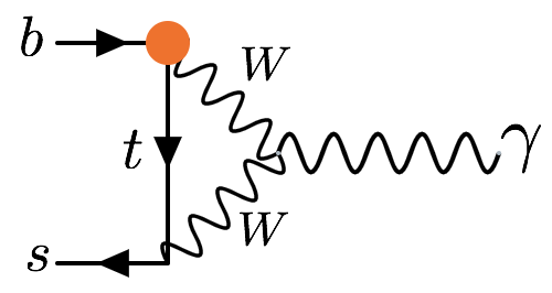
Refer to caption
Refer to caption
Refer to caption
Refer to caption
Refer to caption
Refer to caption
Refer to caption
Figure 7: Diagrams generating contributions to bsγ𝑏𝑠𝛾b\to s\gamma from the QHudsubscript𝑄𝐻𝑢𝑑Q_{Hud} operator.
Refer to caption
Refer to caption
Refer to caption
Refer to caption
Refer to caption
Refer to caption
Refer to caption
Figure 8: Diagrams generating contributions to bsl+l𝑏𝑠superscript𝑙superscript𝑙b\to sl^{+}l^{-} and/or bsγ𝑏𝑠𝛾b\to s\gamma from the QuWsubscript𝑄𝑢𝑊Q_{uW} and QuBsubscript𝑄𝑢𝐵Q_{uB} (3rd and 4th diagrams only) operators. Diagrams in which the operator attaches to the b𝑏b quark leg imply also the existence (and inclusion in our calculations) of similar diagrams with the operator attached to the s𝑠s quark leg.
Refer to caption
Refer to caption
Refer to caption
Refer to caption
Refer to caption
Figure 9: Diagrams generating contributions to bsγ𝑏𝑠𝛾b\to s\gamma from the QdWsubscript𝑄𝑑𝑊Q_{dW} operator.
Refer to caption
Figure 10: Diagram generating contributions to bsγ𝑏𝑠𝛾b\to s\gamma from the operators Qquqd(1)subscriptsuperscript𝑄1𝑞𝑢𝑞𝑑Q^{(1)}_{quqd} and Qquqd(8)subscriptsuperscript𝑄8𝑞𝑢𝑞𝑑Q^{(8)}_{quqd}.

Appendix D Numerical matching results

In this appendix we present the results of our matching calculations in numerical form, as tables of the Nαk(1,2)subscriptsuperscript𝑁12𝛼𝑘N^{(1,2)}_{\alpha k} coefficients of Eqn. (11). The index α𝛼\alpha labels the WET coefficients in the columns of the tables, while the index k𝑘k labels the SMEFT coefficients in the rows. The coefficients Nαk(1)subscriptsuperscript𝑁1𝛼𝑘N^{(1)}_{\alpha k}, which are independent of the choice of input scheme, are given in Table 3, while the coefficients Nαk(2)subscriptsuperscript𝑁2𝛼𝑘N^{(2)}_{\alpha k} are given in Table 4 for the {αem,mZ,GF}subscript𝛼𝑒𝑚subscript𝑚𝑍subscript𝐺𝐹\{\alpha_{em},m_{Z},G_{F}\} input scheme, and in Table 5 for the {mW,mZ,GF}subscript𝑚𝑊subscript𝑚𝑍subscript𝐺𝐹\{m_{W},m_{Z},G_{F}\} input scheme. All table entries are calculated using mt(mt)=163.6subscript𝑚𝑡subscript𝑚𝑡163.6m_{t}(m_{t})=163.6 GeV Marquard:2015qpa , mW=80.379subscript𝑚𝑊80.379m_{W}=80.379 GeV Tanabashi:2018oca , and sin2θW=0.231superscript2subscript𝜃𝑊0.231\sin^{2}\theta_{W}=0.231 Tanabashi:2018oca .

Nαk(1)subscriptsuperscript𝑁1𝛼𝑘N^{(1)}_{\alpha k} C7subscript𝐶7C_{7} C8subscript𝐶8C_{8} C9subscript𝐶9C_{9} C10subscript𝐶10C_{10} CLsubscript𝐶𝐿C_{L}
CWsubscript𝐶𝑊C_{W} - - - - -
CHDsubscript𝐶𝐻𝐷C_{HD} - - -5.16 103absentsuperscript103\cdot 10^{-3} 6.80 102absentsuperscript102\cdot 10^{-2} 1.57 102absentsuperscript102\cdot 10^{-2}
CHWBsubscript𝐶𝐻𝑊𝐵C_{HWB} - - - - -
CuGsubscript𝐶𝑢𝐺C_{uG} - -4.08 102absentsuperscript102\cdot 10^{-2} - - -
CuWsubscript𝐶𝑢𝑊C_{uW} 4.08 102absentsuperscript102\cdot 10^{-2} - - - -
CuBsubscript𝐶𝑢𝐵C_{uB} -7.45 102absentsuperscript102\cdot 10^{-2} - - - -
CdWsubscript𝐶𝑑𝑊C_{dW} -0.163 - - - -
CHl(1)superscriptsubscript𝐶𝐻𝑙1C_{Hl}^{(1)} - - 0.136 -0.136 3.14 102absentsuperscript102\cdot 10^{-2}
CHl(3)superscriptsubscript𝐶𝐻𝑙3C_{Hl}^{(3)} - - -0.136 0.136 3.14 102absentsuperscript102\cdot 10^{-2}
CHesubscript𝐶𝐻𝑒C_{He} - - 0.136 0.136 -
CHq(1)superscriptsubscript𝐶𝐻𝑞1C_{Hq}^{(1)} - - 1.03 102absentsuperscript102\cdot 10^{-2} 0.136 3.14 102absentsuperscript102\cdot 10^{-2}
CHq(3)superscriptsubscript𝐶𝐻𝑞3C_{Hq}^{(3)} - - 7.23 102absentsuperscript102\cdot 10^{-2} -0.951 -0.220
CHusubscript𝐶𝐻𝑢C_{Hu} - - -1.03 102absentsuperscript102\cdot 10^{-2} -0.136 -3.14 102absentsuperscript102\cdot 10^{-2}
CHudsubscript𝐶𝐻𝑢𝑑C_{Hud} - - - - -
Cllsuperscriptsubscript𝐶𝑙𝑙C_{ll}^{\prime} - - - - -
Cqq(1)superscriptsubscript𝐶𝑞𝑞1C_{qq}^{(1)\prime} - - -0.286 1.63 -0.377
Cqq(3)superscriptsubscript𝐶𝑞𝑞3C_{qq}^{(3)\prime} - - 0.286 -1.63 0.377
Cqq(3)superscriptsubscript𝐶𝑞𝑞3C_{qq}^{(3)} - - -0.190 1.09 -0.251
Clq(1)superscriptsubscript𝐶𝑙𝑞1C_{lq}^{(1)} - - 0.136 -0.136 3.14 102absentsuperscript102\cdot 10^{-2}
Clq(3)superscriptsubscript𝐶𝑙𝑞3C_{lq}^{(3)} - - 0.136 0.136 -3.14 102absentsuperscript102\cdot 10^{-2}
Clusubscript𝐶𝑙𝑢C_{lu} - - -0.136 0.136 -3.14 102absentsuperscript102\cdot 10^{-2}
Cqesubscript𝐶𝑞𝑒C_{qe} - - 0.136 0.136 -
Ceusubscript𝐶𝑒𝑢C_{eu} - - -0.136 -0.136 -
Cquqd(1)superscriptsubscript𝐶𝑞𝑢𝑞𝑑1C_{quqd}^{(1)} -1.78 102absentsuperscript102\cdot 10^{-2} -2.68 102absentsuperscript102\cdot 10^{-2} - - -
Cquqd(8)superscriptsubscript𝐶𝑞𝑢𝑞𝑑8C_{quqd}^{(8)} -2.38 102absentsuperscript102\cdot 10^{-2} 4.46 103absentsuperscript103\cdot 10^{-3} - - -
Cquqd(1)superscriptsubscript𝐶𝑞𝑢𝑞𝑑1C_{quqd}^{(1)\prime} -2.97 102absentsuperscript102\cdot 10^{-2} -4.46 103absentsuperscript103\cdot 10^{-3} - - -
Cquqd(8)superscriptsubscript𝐶𝑞𝑢𝑞𝑑8C_{quqd}^{(8)\prime} -7.93 103absentsuperscript103\cdot 10^{-3} -2.52 102absentsuperscript102\cdot 10^{-2} - - -
Table 3: Numerical values of the coefficients Nαk(1)subscriptsuperscript𝑁1𝛼𝑘N^{(1)}_{\alpha k} of the matching equation Eqn. (11). Note that the matching to C1,mixsubscript𝐶1mixC_{1,\text{mix}}, C1subscript𝐶1C_{1} and C2subscript𝐶2C_{2} does not have any divergent diagrams so the corresponding Nαk(1)subscriptsuperscript𝑁1𝛼𝑘N^{(1)}_{\alpha k} coefficients are all zero (and are not listed here). All results are quark-flavour universal (CαCαbs=Cαbd=Cαsdsubscript𝐶𝛼superscriptsubscript𝐶𝛼𝑏𝑠superscriptsubscript𝐶𝛼𝑏𝑑superscriptsubscript𝐶𝛼𝑠𝑑C_{\alpha}\equiv C_{\alpha}^{bs}=C_{\alpha}^{bd}=C_{\alpha}^{sd}), except for results indicated by an asterisk (), for which only Cαbdjsuperscriptsubscript𝐶𝛼𝑏subscript𝑑𝑗C_{\alpha}^{bd_{j}} is meant (dj=s,dsubscript𝑑𝑗𝑠𝑑d_{j}=s,d).
Nαk(2)subscriptsuperscript𝑁2𝛼𝑘N^{(2)}_{\alpha k} C1subscript𝐶1C_{1} C2subscript𝐶2C_{2} C7subscript𝐶7C_{7} C8subscript𝐶8C_{8} C9subscript𝐶9C_{9} C10subscript𝐶10C_{10} CLsubscript𝐶𝐿C_{L} C1,mix(xt)subscript𝐶1mixsubscript𝑥𝑡C_{1,\text{mix}}(x_{t})
CWsubscript𝐶𝑊C_{W} - - -1.68 103absentsuperscript103\cdot 10^{-3} - -4.92 102absentsuperscript102\cdot 10^{-2} - - -
CHDsubscript𝐶𝐻𝐷C_{HD} - - 9.48 103absentsuperscript103\cdot 10^{-3} - 0.260 4.75 102absentsuperscript102\cdot 10^{-2} 1.10 102absentsuperscript102\cdot 10^{-2} -
CHWBsubscript𝐶𝐻𝑊𝐵C_{HWB} - - 1.30 101absentsuperscript101\cdot 10^{-1} - 0.398 - - -
CuGsubscript𝐶𝑢𝐺C_{uG} - - - -2.94 102absentsuperscript102\cdot 10^{-2} - - - -
CuWsubscript𝐶𝑢𝑊C_{uW} - - 4.88 103absentsuperscript103\cdot 10^{-3} 1.60 102absentsuperscript102\cdot 10^{-2} 0.102 -0.383 0.157 0.215
CuBsubscript𝐶𝑢𝐵C_{uB} - - -5.37 102absentsuperscript102\cdot 10^{-2} - 0.137 - - -
CdWsubscript𝐶𝑑𝑊C_{dW} - - 3.33 102absentsuperscript102\cdot 10^{-2} 5.33 102absentsuperscript102\cdot 10^{-2} - - - -
CHl(1)superscriptsubscript𝐶𝐻𝑙1C_{Hl}^{(1)} - - - - 9.50 102absentsuperscript102\cdot 10^{-2} -9.50 102absentsuperscript102\cdot 10^{-2} 2.20 102absentsuperscript102\cdot 10^{-2} -
CHl(3)superscriptsubscript𝐶𝐻𝑙3C_{Hl}^{(3)} - - 3.42 102absentsuperscript102\cdot 10^{-2} 1.15 102absentsuperscript102\cdot 10^{-2} -4.03 102absentsuperscript102\cdot 10^{-2} 0.594 -0.203 -1.13
CHesubscript𝐶𝐻𝑒C_{He} - - - - 9.50 102absentsuperscript102\cdot 10^{-2} 9.50 102absentsuperscript102\cdot 10^{-2} - -
CHq(1)superscriptsubscript𝐶𝐻𝑞1C_{Hq}^{(1)} - - - - 7.22 103absentsuperscript103\cdot 10^{-3} 9.50 102absentsuperscript102\cdot 10^{-2} 2.20 102absentsuperscript102\cdot 10^{-2} -
CHq(3)superscriptsubscript𝐶𝐻𝑞3C_{Hq}^{(3)} - - -2.28 102absentsuperscript102\cdot 10^{-2} -1.15 102absentsuperscript102\cdot 10^{-2} 0.273 -1.71 -0.275 0.564
CHusubscript𝐶𝐻𝑢C_{Hu} - - - - -7.22 103absentsuperscript103\cdot 10^{-3} -9.50 102absentsuperscript102\cdot 10^{-2} -2.20 102absentsuperscript102\cdot 10^{-2} -
CHudsubscript𝐶𝐻𝑢𝑑C_{Hud} - - -2.12 102absentsuperscript102\cdot 10^{-2} -9.46 103absentsuperscript103\cdot 10^{-3} - - - -
Cllsuperscriptsubscript𝐶𝑙𝑙C_{ll}^{\prime} - - -1.71 102absentsuperscript102\cdot 10^{-2} -5.76 103absentsuperscript103\cdot 10^{-3} 0.363 -0.498 -0.181 0.564
Cqq(1)superscriptsubscript𝐶𝑞𝑞1C_{qq}^{(1)\prime} -6.06 102absentsuperscript102\cdot 10^{-2} - - - -0.203 1.16 0.268 -0.251
Cqq(3)superscriptsubscript𝐶𝑞𝑞3C_{qq}^{(3)\prime}  6.06 102absentsuperscript102\cdot 10^{-2} - - - 0.203 -1.16 -0.268 0.251
Cqq(3)superscriptsubscript𝐶𝑞𝑞3C_{qq}^{(3)} - -0.121 - - -0.231 1.32 0.304 -0.503
Clq(1)superscriptsubscript𝐶𝑙𝑞1C_{lq}^{(1)} - - - - 0.125 -9.50 102absentsuperscript102\cdot 10^{-2} 2.20 102absentsuperscript102\cdot 10^{-2} -
Clq(3)superscriptsubscript𝐶𝑙𝑞3C_{lq}^{(3)} - - - - -0.177 -0.176 4.08 102absentsuperscript102\cdot 10^{-2} -
Clusubscript𝐶𝑙𝑢C_{lu} - - - - -9.50 102absentsuperscript102\cdot 10^{-2} 9.50 102absentsuperscript102\cdot 10^{-2} -2.65 102absentsuperscript102\cdot 10^{-2} -
Cqesubscript𝐶𝑞𝑒C_{qe} - - - - 9.50 102absentsuperscript102\cdot 10^{-2} 9.50 102absentsuperscript102\cdot 10^{-2} - -
Ceusubscript𝐶𝑒𝑢C_{eu} - - - - -9.50 102absentsuperscript102\cdot 10^{-2} -9.50 102absentsuperscript102\cdot 10^{-2} - -
Cquqd(1)superscriptsubscript𝐶𝑞𝑢𝑞𝑑1C_{quqd}^{(1)} - - -1.26 102absentsuperscript102\cdot 10^{-2} -1.90 102absentsuperscript102\cdot 10^{-2} - - - -
Cquqd(8)superscriptsubscript𝐶𝑞𝑢𝑞𝑑8C_{quqd}^{(8)} - - -1.69 102absentsuperscript102\cdot 10^{-2} 3.17 103absentsuperscript103\cdot 10^{-3} - - - -
Cquqd(1)superscriptsubscript𝐶𝑞𝑢𝑞𝑑1C_{quqd}^{(1)\prime} - - -2.11 102absentsuperscript102\cdot 10^{-2} -3.17 103absentsuperscript103\cdot 10^{-3} - - - -
Cquqd(8)superscriptsubscript𝐶𝑞𝑢𝑞𝑑8C_{quqd}^{(8)\prime} - - -5.63 103absentsuperscript103\cdot 10^{-3} -1.80 102absentsuperscript102\cdot 10^{-2} - - - -
Table 4: Numerical values of the coefficients Nαk(2)subscriptsuperscript𝑁2𝛼𝑘N^{(2)}_{\alpha k} of the matching equation Eqn. (11), in the {mW,mZ,GF}subscript𝑚𝑊subscript𝑚𝑍subscript𝐺𝐹\{m_{W},m_{Z},G_{F}\} input scheme. All results are quark-flavour universal (CαCαbs=Cαbd=Cαsdsubscript𝐶𝛼superscriptsubscript𝐶𝛼𝑏𝑠superscriptsubscript𝐶𝛼𝑏𝑑superscriptsubscript𝐶𝛼𝑠𝑑C_{\alpha}\equiv C_{\alpha}^{bs}=C_{\alpha}^{bd}=C_{\alpha}^{sd}), except for results indicated by an asterisk (), for which only Cαbdjsuperscriptsubscript𝐶𝛼𝑏subscript𝑑𝑗C_{\alpha}^{bd_{j}} is meant (dj=s,dsubscript𝑑𝑗𝑠𝑑d_{j}=s,d).
Nαk(2)subscriptsuperscript𝑁2𝛼𝑘N^{(2)}_{\alpha k} C1subscript𝐶1C_{1} C2subscript𝐶2C_{2} C7subscript𝐶7C_{7} C8subscript𝐶8C_{8} C9subscript𝐶9C_{9} C10subscript𝐶10C_{10} CLsubscript𝐶𝐿C_{L} C1,mix(xt)subscript𝐶1mixsubscript𝑥𝑡C_{1,\text{mix}}(x_{t})
CWsubscript𝐶𝑊C_{W} - - -1.68 102absentsuperscript102\cdot 10^{-2} - -4.92 102absentsuperscript102\cdot 10^{-2} - - -
CHDsubscript𝐶𝐻𝐷C_{HD} - - 7.71 103absentsuperscript103\cdot 10^{-3} 5.61 103absentsuperscript103\cdot 10^{-3} -0.156 8.73 102absentsuperscript102\cdot 10^{-2} 3.93 102absentsuperscript102\cdot 10^{-2} -
CHWBsubscript𝐶𝐻𝑊𝐵C_{HWB} - - -1.68 102absentsuperscript102\cdot 10^{-2} 1.23 102absentsuperscript102\cdot 10^{-2} -0.382 8.73 102absentsuperscript102\cdot 10^{-2} 6.29 102absentsuperscript102\cdot 10^{-2} -
CuGsubscript𝐶𝑢𝐺C_{uG} - - - -2.94 102absentsuperscript102\cdot 10^{-2} - - - -
CuWsubscript𝐶𝑢𝑊C_{uW} - - 4.88 103absentsuperscript103\cdot 10^{-3} 1.60 102absentsuperscript102\cdot 10^{-2} 0.102 -0.383 0.157 0.215
CuBsubscript𝐶𝑢𝐵C_{uB} - - -5.37 102absentsuperscript102\cdot 10^{-2} - 0.137 - - -
CdWsubscript𝐶𝑑𝑊C_{dW} - - -3.33 103absentsuperscript103\cdot 10^{-3} 5.33 102absentsuperscript102\cdot 10^{-2} - - - -
CHl(1)superscriptsubscript𝐶𝐻𝑙1C_{Hl}^{(1)} - - - - 9.50 102absentsuperscript102\cdot 10^{-2} -9.50 102absentsuperscript102\cdot 10^{-2} 2.20 102absentsuperscript102\cdot 10^{-2} -
CHl(3)superscriptsubscript𝐶𝐻𝑙3C_{Hl}^{(3)} - - -0.204 -4.20 103absentsuperscript103\cdot 10^{-3} 0.211 1.39 -0.350 -1.13
CHesubscript𝐶𝐻𝑒C_{He} - - - - 9.50 102absentsuperscript102\cdot 10^{-2} 9.50 102absentsuperscript102\cdot 10^{-2} - -
CHq(1)superscriptsubscript𝐶𝐻𝑞1C_{Hq}^{(1)} - - - - 7.22 103absentsuperscript103\cdot 10^{-3} 9.50 102absentsuperscript102\cdot 10^{-2} 2.20 102absentsuperscript102\cdot 10^{-2} -
CHq(3)superscriptsubscript𝐶𝐻𝑞3C_{Hq}^{(3)} - - -2.28 102absentsuperscript102\cdot 10^{-2} -1.15 102absentsuperscript102\cdot 10^{-2} 0.273 -1.71 -0.275 0.564
CHusubscript𝐶𝐻𝑢C_{Hu} - - - - -7.22 103absentsuperscript103\cdot 10^{-3} -9.50 102absentsuperscript102\cdot 10^{-2} -2.20 102absentsuperscript102\cdot 10^{-2} -
CHudsubscript𝐶𝐻𝑢𝑑C_{Hud} - - -2.12 102absentsuperscript102\cdot 10^{-2} -9.46 103absentsuperscript103\cdot 10^{-3} - - - -
Cllsuperscriptsubscript𝐶𝑙𝑙C_{ll}^{\prime} - - 0.102 2.10 103absentsuperscript103\cdot 10^{-3} 0.278 -0.899 -0.254 0.564
Cqq(1)superscriptsubscript𝐶𝑞𝑞1C_{qq}^{(1)\prime} -6.06 102absentsuperscript102\cdot 10^{-2} - - -0.203 1.16 0.268 -0.251
Cqq(3)superscriptsubscript𝐶𝑞𝑞3C_{qq}^{(3)\prime} - 6.06 102absentsuperscript102\cdot 10^{-2} - - 0.203 -1.16 -0.268 0.251
Cqq(3)superscriptsubscript𝐶𝑞𝑞3C_{qq}^{(3)} - -0.121 - - -0.231 1.32 0.304 -0.503
Clq(1)superscriptsubscript𝐶𝑙𝑞1C_{lq}^{(1)} - - - - 0.125 -9.50 102absentsuperscript102\cdot 10^{-2} 2.20 102absentsuperscript102\cdot 10^{-2} -
Clq(3)superscriptsubscript𝐶𝑙𝑞3C_{lq}^{(3)} - - - - -0.177 -0.176 4.08 102absentsuperscript102\cdot 10^{-2} -
Clusubscript𝐶𝑙𝑢C_{lu} - - - - -9.50 102absentsuperscript102\cdot 10^{-2} 9.50 102absentsuperscript102\cdot 10^{-2} -2.65 102absentsuperscript102\cdot 10^{-2} -
Cqesubscript𝐶𝑞𝑒C_{qe} - - - - 9.50 102absentsuperscript102\cdot 10^{-2} 9.50 102absentsuperscript102\cdot 10^{-2} - -
Ceusubscript𝐶𝑒𝑢C_{eu} - - - - -9.50 102absentsuperscript102\cdot 10^{-2} -9.50 102absentsuperscript102\cdot 10^{-2} - -
Cquqd(1)superscriptsubscript𝐶𝑞𝑢𝑞𝑑1C_{quqd}^{(1)} - - -1.27 102absentsuperscript102\cdot 10^{-2} -1.90 102absentsuperscript102\cdot 10^{-2} - - - -
Cquqd(8)superscriptsubscript𝐶𝑞𝑢𝑞𝑑8C_{quqd}^{(8)} - - -1.69 102absentsuperscript102\cdot 10^{-2} 3.17 103absentsuperscript103\cdot 10^{-3} - - - -
Cquqd(1)superscriptsubscript𝐶𝑞𝑢𝑞𝑑1C_{quqd}^{(1)\prime} - - -2.11 102absentsuperscript102\cdot 10^{-2} -3.17 103absentsuperscript103\cdot 10^{-3} - - - -
Cquqd(8)superscriptsubscript𝐶𝑞𝑢𝑞𝑑8C_{quqd}^{(8)\prime} - - -5.64 103absentsuperscript103\cdot 10^{-3} -1.80 102absentsuperscript102\cdot 10^{-2} - - - -
Table 5: Numerical values of the coefficients Nαk(2)subscriptsuperscript𝑁2𝛼𝑘N^{(2)}_{\alpha k} of the matching equation Eqn. (11), in the {αem,mZ,GF}subscript𝛼𝑒𝑚subscript𝑚𝑍subscript𝐺𝐹\{\alpha_{em},m_{Z},G_{F}\} input scheme. All results are quark-flavour universal (CαCαbs=Cαbd=Cαsdsubscript𝐶𝛼superscriptsubscript𝐶𝛼𝑏𝑠superscriptsubscript𝐶𝛼𝑏𝑑superscriptsubscript𝐶𝛼𝑠𝑑C_{\alpha}\equiv C_{\alpha}^{bs}=C_{\alpha}^{bd}=C_{\alpha}^{sd}), except for results indicated by an asterisk (), for which only Cαbdjsuperscriptsubscript𝐶𝛼𝑏subscript𝑑𝑗C_{\alpha}^{bd_{j}} is meant (dj=s,dsubscript𝑑𝑗𝑠𝑑d_{j}=s,d).