Adaptive Neural Trajectory Tracking Control for Flexible-Joint
Robots with Online Learning

Abstract

Collaborative robots and space manipulators contain significant joint flexibility. It complicates the control design, compromises the control bandwidth, and limits the tracking accuracy. The imprecise knowledge of the flexible joint dynamics compounds the challenge. In this paper, we present a new control architecture for controlling flexible-joint robots. Our approach uses a multi-layer neural network to approximate unknown dynamics needed for the feedforward control. The network may be viewed as a linear-in-parameter representation of the robot dynamics, with the nonlinear basis of the robot dynamics connected to the linear output layer. The output layer weights are updated based on the tracking error and the nonlinear basis. The internal weights of the nonlinear basis are updated by online backpropagation to further reduce the tracking error. To use time scale separation to reduce the coupling of the two steps – the update of the internal weights is at a lower rate compared to the update of the output layer weights. With the update of the output layer weights, our controller adapts quickly to the unknown dynamics change and disturbances (such as attaching a load). The update of the internal weights would continue to improve the converge of the nonlinear basis functions. We show the stability of the proposed scheme under the “outer loop” control, where the commanded joint position is considered as the control input. Simulation and physical experiments are conducted to demonstrate the performance of the proposed controller on a Baxter robot, which exhibits significant joint flexibility due to the series-elastic joint actuators.

I INTRODUCTION

Robot manipulators are playing important roles in an increasing range of applications such as material handling, assembly, surface finishing, surgery, and in-space satellite servicing. There has been numerous work on the trajectory tracking control of robot manipulators [1]. If the robot dynamics is expressed in the linear-in-parameter form, adaptive controller has been developed to achieve asymptotic tracking [2]. However, accurate dynamics models of robot manipulators are rarely available, particularly for flexible-joint manipulators. For such robots, a simplified reduced-order model may be used [3] for feedforward control, with model parameters obtained from offline identification. For rigid robots, iterative learning control (ILC) [4] has been applied for tracking specific trajectories, but the learned representation is not transferable to new trajectories. Neural network (NN) based controller demonstrates high generalization capability to new trajectories given enough training data and carefully designed architecture [5]. These control approaches have been extended to flexible-joint robots [6, 7, 8], but the control performance is sacrificed to guarantee safety, especially for the high speed motion.

Numerous schemes have been proposed to control a robot with unknown dynamics, and examples include dynamics approximation by wavelet networks [9], Gaussian Processes [10], Locally Weighted Projection Regression (LWPR), fuzzy logic systems [11] and neural networks [12]. NNs are used to either approximate the robot forward dynamics [13] or inverse dynamics [14] for the controller design. In our previous work [15], we developed two feedforward controllers using recurrent neural networks (RNNs) to compensate for the unknown dynamics of a Baxter robot. One controller was based on a unidirectional RNN that approximates the forward dynamics of Baxter and the other controller was based on a bidirectional RNN that approximates the non-causal dynamical system inverse of Baxter. Though the approach has demonstrated good tracking results, there are several drawbacks. The RNNs require a large amount of training data to obtain a satisfactory approximation of the robot dynamics. The approach also lacks a rigorous trajectory error convergence proof and stability analysis. In addition, the NNs were trained offline with no online updates. Similarly, in [16], we trained a multi-layer feedforward NN to approximate the dynamical inverse of an ABB industrial robot with training data collected by implementing ILC with a large amount of trajectories. The trained NN performed well in compensating for the unseen trajectories but has the similar issues to [15]. In [17], feedforward NNs and RNNs were evaluated for identification and control of structured dynamical systems. The parameters of NNs were updated by online backpropagation and controllers were designed using the trained NNs. The parameters update of NNs and controller implementation were conducted simultaneously but at different rates. However, no stability proof was provided. A survey of neural-learning robot manipulators control can be referred to in [18].

Adaptive control [2] has long been used to achieve globally asymptotically trajectory tracking and the approach is based on expressing robot dynamics in a linear-in-parameter form. Essentially, it linearizes the system through controller online adaptation to cancel the nonlinear dynamics. Neural network is a natural candidate to approximate the robot dynamics for adaptive controllers development [19]. A popular choice is the radial basis function (RBF) NN [20, 21] since it naturally expresses the approximation linearly in the parameters. In [22], an adaptive controller was developed based on RBF NNs to compensate for the unknown dynamics and payload for a Baxter robot. The controller produced control inputs in the joint-torque level. However, for many industrial robots, users have only access to the joint position or velocity setpoint control. Further, it is non-trivial to select the centers and shapes of radial basis functions, and typically a large amount of Gaussian kernels are required to approximate the complex robot dynamics accurately. Finally, some properties of robot dynamics cannot be guaranteed with individual RBF NN approximation, such as the positive definiteness of the inertia matrix and passivity. In [23, 24], an adaptive controller in the joint-torque level based on a two-layer feedforward perceptron NN was developed for control of robot manipulators with a guaranteed tracking performance. The dynamics approximation was nonlinear in the unknown parameters and Taylor series expansion was used for development of the parameters adaptation law. A robust control term was introduced to overcome the NN approximation errors and system uncertainties. With more NN layers, the adaptation law derivation would be far more complex. Other proposed control frameworks that use general function approximators to learn system dynamics for linearizing controllers design can be referred to in [25, 26, 27].

Figure 1: Overall control architecture.

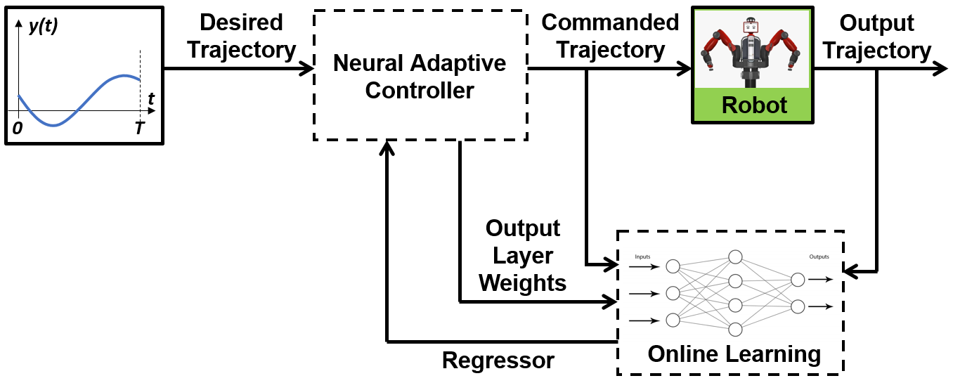
This paper presents a novel neural adaptive controller for the tracking control of a flexible-joint robot under the outer-loop control. Fig. 1 shows the schematics of the control architecture. We design a network which is composed of a regressor network and an output layer. Thus the NN parameters can be classified into two categories: the internal weights of the regressor, and the output layer weights. The goal is to use the network to emulate the linear-in-parameter form of the robot dynamics. The updates of the internal and output layer weights are parallel and coupled, and operating at different time scales. The output layer weights are updated at a fast rate by the adaptation law developed from the Lyapunov analysis, and the internal weights are updated slowly via online backpropagation using collected robot input/output data. During the backpropagation, the output layer weights of the network remain fixed so that only the regressor weights are updated. The updated regressor is then involved in the output layer weights adaptation. This time scale separation of the internal and output layer parameters is inspired by the singular perturbation theory.

The rest of the paper is organized as follows. Section II states the problem, followed by the description of controller design in Section III. The simulation and physical robot experimental results are presented in Sections IV and V, respectively. Finally, Section VI concludes the paper.

II Problem Statement

We consider the trajectory tracking control problem for a flexible-joint robot manipulator modeled as [20, 21]:

$$\begin{split}M(\theta)\ddot{\theta}+C(\theta,\dot{\theta})\dot{\theta}+G(\theta)+K\cdot(\theta-\theta_{m})=0\\ J_{m}{\ddot{\theta}}_{m}+K\cdot(\theta_{m}-\theta)=\tau,\end{split}$$ (1)

where $\theta,\theta_{m}$ are the link position and motor position. $M(\theta),C(\theta,\dot{\theta})\dot{\theta},G(\theta)$ denote the manipulator inertia matrix ($M$ is symmetric positive definite and $\dot{M}-2C$ is skew-symmetric), Coriolis and centrifugal torques, and gravitational torques, respectively. $\tau$ is the motor torque input, and $J_{m}$ and $K$ are constant diagonal and positive definite matrices representing the motor inertia and joint stiffness. To simplify the analysis, we make the following assumptions:

• The motor position $\theta_{m}$ is perfectly controlled, i.e., we can ignore the motor dynamics and use $\theta_{m}$ as an input to drive $\theta$.

• Joint stiffness is the same for all joints, i.e., $K=k_{p}I$, $k_{p}>0$.

The robot dynamics can be rewritten as

$$M(\theta)\ddot{\theta}+C(\theta,\dot{\theta})\dot{\theta}+H(\theta)=k_{p}\theta_{m},$$ (2)

where $H(\theta)=G(\theta)+k_{p}\theta$. We then express the dynamics into a linear-in-parameter form as follows:

$$Y(\dot{\theta}_{1},\theta,\dot{\theta}_{2},\ddot{\theta})a:=k_{p}^{-1}(M(\theta)\ddot{\theta}+C(\theta,\dot{\theta}_{2})\dot{\theta}_{1}+H(\theta)),$$ (3)

where $Y$ is the regressor and $a$ is a constant vector. Our goal is to design an adaptive controller for $\theta_{m}$ that achieves globally asymptotically tracking of a desired trajectory $\theta_{d}$ with bounded first and second-order time derivatives. We will first test the approach in simulation with a single pendulum, and then extend it to a multi-link robot such as the Baxter and compare the performance of the adaptive controller with a baseline proportional-derivative (PD) controller (with gains $K_{1}$ and $K_{2}$) as below:

$$\theta_{m}=\theta_{d}-K_{1}(\theta-\theta_{d})-K_{2}(\dot{\theta}-\dot{\theta}_{d}).$$ (4)

Finally, we compare the adaptive controller with and without the online regressor backpropagation to demonstrate the feasibility of the proposed regressor online learning scheme.

III Neural Adaptive Controller

In this section, we propose a network architecture and design an adaptive controller that achieves asymptotically trajectory tracking for the robot manipulators modeled in (2).

III-A Controller Design

For the controller derivation, we use the following Lyapunov-like function candidate for stability analysis. The design of NN architecture naturally arises during the stability analysis.

$$V=\frac{1}{2}s^{T}Ms+\frac{1}{2}\widetilde{a}^{T}k_{p}P^{-1}\widetilde{a},$$ (5)

where $M$ and $k_{p}$ are the robot inertia matrix and joint stiffness in (2) and $s$ is a sliding vector where $s=\dot{e}(t)+\Lambda e(t)$ with $e(t)=\theta(t)-\theta_{d}(t)$. $\widetilde{a}=\hat{a}-a$ and $\hat{a}$ is an estimate of the constant vector $a$. The designed weighting matrix $P$ controls the parameter adaptation rate and is symmetric and positive definite. The Hurwitz matrix $-\Lambda$ makes $e(t),\dot{e}(t)$ converge to zero exponentially as $s$ converges to zero. $\theta_{r}$ is defined so that $s=\dot{\theta}-\dot{\theta}_{r}$ (i.e., $\dot{\theta}_{r}=\dot{\theta}_{d}-\Lambda e)$.

By taking the time derivative of $V$ and from (2) and (3), we have:

$$\begin{split}&\dot{V}=s^{T}M\dot{s}+\frac{1}{2}s^{T}\dot{M}s+\dot{\hat{a}}^{T}k_{p}P^{-1}\tilde{a}\\ &=s^{T}(M\ddot{\theta}-M\ddot{\theta}_{r})+\frac{1}{2}s^{T}\dot{M}s+\dot{\hat{a}}^{T}k_{p}P^{-1}\tilde{a}\\ &=s^{T}(k_{p}\theta_{m}-H-C\dot{\theta}-M\ddot{\theta}_{r})+\frac{1}{2}s^{T}\dot{M}s+\dot{\hat{a}}^{T}k_{p}P^{-1}\tilde{a}\\ &=s^{T}(k_{p}\theta_{m}-H-C\dot{\theta}_{r}-M\ddot{\theta}_{r})+\frac{1}{2}s^{T}(\dot{M}-2C)s\\ &\qquad\qquad+\dot{\hat{a}}^{T}k_{p}P^{-1}\tilde{a}\\ &=s^{T}(k_{p}\theta_{m}-H-C\dot{\theta}_{r}-M\ddot{\theta}_{r})+\dot{\hat{a}}^{T}k_{p}P^{-1}\tilde{a}\\ &=s^{T}k_{p}(\theta_{m}-Y(\dot{\theta}_{r},\theta,\dot{\theta},\ddot{\theta}_{r})a)+\dot{\hat{a}}^{T}k_{p}P^{-1}\tilde{a}.\end{split}$$ (6)

If $Y$ is known, then we may design $\theta_{m}$ to cancel $Ya$ using the estimate $\hat{a}$ as

$$\theta_{m}=Y(\dot{\theta}_{r},\theta,\dot{\theta},\ddot{\theta}_{r})\hat{a}-K_{s}s-k{\mbox{\bf sgn}}(s).$$ (7)

The $K_{s}s$ term with $K_{s}>0$ ensures the tracking error convergence. The additional high gain feedback term $k{\mbox{\bf sgn}}(s)$ provides robustness with respect to the network modeling errors and noises. It follows

$$\dot{V}=-s^{T}k_{p}K_{s}s-kk_{p}\left\|{s}\right\|_{1}+k_{p}s^{T}Y\tilde{a}+k_{p}{\dot{\hat{a}}}^{T}P^{-1}\tilde{a},$$ (8)

where $\left\|{\cdot}\right\|_{1}$ denotes the vector 1-norm. By choosing the adaptation law of $\hat{a}$ as

$$\dot{\hat{a}}=-PY^{T}(\dot{\theta}_{r},\theta,\dot{\theta},\ddot{\theta}_{r})s,$$ (9)

we have

$$\dot{V}=-s^{T}k_{p}K_{s}s-kk_{p}\left\|{s}\right\|_{1}.$$ (10)

This implies $s\to 0$ asymptotically which in turn implies $e\to 0$ asymptotically. In the next section, we design a neural network architecture to approximate $Y(\dot{\theta}_{r},\theta,\dot{\theta},\ddot{\theta}_{r})a$.

III-B Neural Network Design

III-B1 Network Architecture

Figure 2: Network architecture.

TABLE I: Neural network connections.

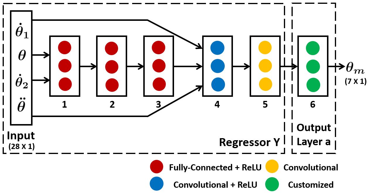
Layer Number	Learnable Size	Output Size
1	Weights: $100\times$14	100$\times$1
	Bias: $100\times$1
2	Weights: $100\times$100	100$\times$1
	Bias: $100\times$1
3	Weights: $7\times$100	7$\times$1
	Bias: $7\times$1
4	Weights: $1\times$1$\times$3$\times$100	7$\times$1$\times$100
	Bias: 1$\times$1$\times$100
5	Weights: $1\times$1$\times$100$\times$200	7$\times$1$\times$200
	Bias: 1$\times$1$\times$200
6	Weights: $200\times$1	7$\times$1

We design a network as a directed acrylic graph composed of different layers, as presented in Fig. 2. Table. I summarizes the connections between consecutive layers. The regressor network $Y(\dot{\theta}_{1},\theta,\dot{\theta}_{2},\ddot{\theta})$ has its own internal weights from the fully-connected layers and convolutional layers, and $a$ is an $N-$parameter output layer which is compatible with the output dimension of $Y$. Note that we need one convolutional layer (the yellow block in Fig. 2) instead of a fully-connected layer as the final layer of $Y$, as the size of output of $Y$ is 2-dimensional (7 by $N$) for a 7-joint robot, whereas a fully-connected layer only provides a 1-dimensional vector output. Thus, for a single-input and single-output (SISO) system such as a single pendulum, the last layer of $Y$ is a fully-connected layer.

III-B2 Training Data Collection

We collect data from the left arm of the Baxter robot by commanding 30 sinusoidal trajectories $\theta_{m}$ with different magnitudes and frequencies. We choose the trajectories by obeying the Baxter joint limits and also try to cover a feasible portion of its joint workspace. Each trajectory contains 2500 joint position setpoints for all 7 joints (thus a 7 by 2500 matrix) and is commanded to Baxter at 100 Hz. The output joint position trajectory $\theta$ as well as the joint velocity trajectory $\dot{\theta}$ are collected at the same rate. The joint acceleration trajectory $\ddot{\theta}$ is approximated by cubic spline interpolation of the joint velocity trajectory.

III-B3 Network Training for Initialization

During training, the input to the network is $(\dot{\theta}(t),\theta(t),\dot{\theta}(t),\ddot{\theta}(t))$, and the output of the network is the commanded position $\theta_{m}(t)$. We use 80 % of the collected data for network training and 20 % for testing. We use AdamOptimizer with an initial learning rate of $1\times 10^{-3}$ to tune the parameters of the network by minimizing the mean squared error (MSE) between the predicted output and the actual output over a randomly selected batch of 256 samples in each training iteration. We use $L_{2}$ regularization (penalizing large weights) to avoid overfitting. The training process converges after 5 epochs. After the initial network training, we use the output of the neural network with input of $(\dot{\theta}_{r},\theta,\dot{\theta},\ddot{\theta}_{r})$ as $Y\hat{a}$ to implement the controller in (7). The output layer weights are then updated using (9). On a slower time scale, the regressor $Y$ is updated using online backpropagation with regularization. Note that the network provides an estimate of the complete $Y$ matrix, so we may use $Y^{T}$ directly in the update law (9).

III-C Online Backpropagation for Regressor Update

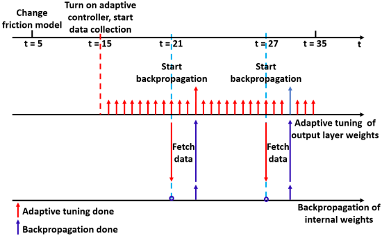
When the system is subject to dynamics variation (e.g., attaching a load and friction change) and external disturbances, pure adaptation of output layer weights by (9) may take a long time to make the tracking error converge. Here, we explore the online learning of regressor $Y$ with the collected input/output data of the system after dynamics variation. We update the output layer weights at a higher rate, whereas the regressor weights are updated at a lower rate inspired by the singular perturbation theory. When updating the regressor, we fetch and freeze the values of the output layer weights and only update the regressor weights by backpropagation of the entire network. Then the updated regressor is utilized in (7) and (9). An example of using time scale separation for the regressor online learning is illustrated in Fig. 3.

Figure 3: Schematics of the regressor online learning.

IV Simulation

To demonstrate the feasibility of the proposed controller with the regressor online learning scheme, we first simulate the scenario that the internal friction model changes from viscous and Coulomb friction to Stribeck friction of a single pendulum modeled in Simulink. The system dynamics is based on (1) and the assumption that $K$ is a scalar naturally holds for this SISO system. Then, we test the approach with MIMO systems through physical experiments.

We collect 6000 training data sets ($\theta_{m},\theta,\dot{\theta},\ddot{\theta}$) from the single pendulum by commanding a Schroeder-phase multisine signal to the system. Then, a network with architecture denoted in Fig. 2 is trained using MATLAB Deep Learning Toolbox with the following variations: first, the input size of the network is 4 by 1 and the output size is 1 by 1; second, the last layer of the regressor is a fully-connected layer instead of a convolutional layer, considering that the single pendulum is an SISO system. We simulate the following scenario for two systems with the same single pendulum model and the trained network, but in one system we implement regressor online learning (system I), and as a comparison in system II, no online learning is conducted. The same single pendulum in two systems is commanded to track a sinusoidal trajectory following the procedures as below:

• From $t=0\sim 5~{}s$, for both systems I and II, we implement the controller in (7) with the trained network but without the adaptation of $\hat{a}$ in (9). The value of $\hat{a}$ remains fixed and is from the initial value of the trained network.

• At $t=5~{}s$, for both systems we change the friction model and with the same controller implemented as above.

• At $t=15~{}s$, we turn on the adaptive controller (with adaptation law in (9) activated) for both systems. We start collecting the input/output data of system I with the modified dynamics model.

• At $t=21~{}s$, we start conducting the regressor online learning for system I using the collected input/output data every 6 seconds until end of the simulation. The first, second and third online updates complete at around $t=21.5~{}s$, $t=27.5~{}s$, and $t=33.5~{}s$, respectively. Note that the controller in (7) keeps activated during the entire simulation for both systems.

Figure 4: Comparison of absolute tracking errors of a sinusoidal trajectory for the single pendulum with and without online backpropagation of the regressor. The large errors from $t=0\sim 2~{}s$ (the initial tracking error is 0.25 radian at $t=0$ and the mean error is 0.0461 radian from $t=0\sim 2~{}s$) are not plotted to better visualize the later small errors.

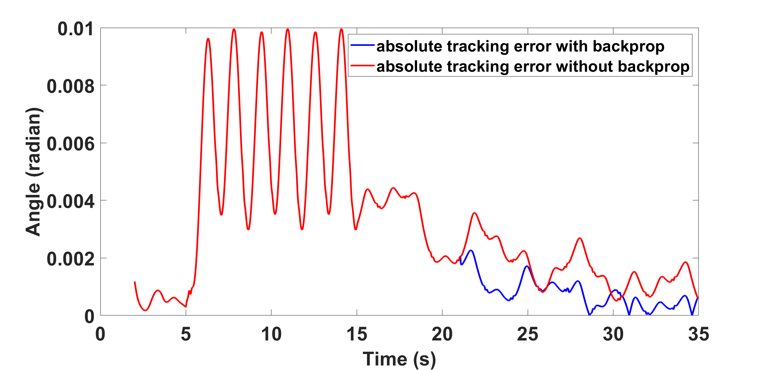
Figure 3 illustrates the timeline of system I in the simulation. The comparison of absolute tracking error in radian of two systems over the entire process is presented in Fig. 4. We do not plot the large initial tracking errors during $t=0\sim 2~{}s$ to better visualize the later smaller tracking errors.

The figure demonstrates the following stages:

• The tracking errors converge for both systems from $t=0\sim 5~{}s$, which means our trained network approximates the single pendulum dynamics model accurately.

• From $t=5\sim 15~{}s$, the tracking errors of both systems increase due to the change of the friction model.

• Once we turn on the adaptive controller at $t=15~{}s$, the controller reduces the tracking errors for both systems. However, for system I, the tracking error is further reduced with the complete of regressor update via online backpropagation.

V Experiment with Baxter

After an initial training of a network with architecture illustrated in Fig. 2, the testing of the control framework for MIMO systems such as a Baxter robot is composed of two parts. The first one is a feasibility study, in which we show the feasibility of our assumptions in Section II by commanding the Baxter to track an unseen multi-joint sinusoidal trajectory and compare the tracking performance of the adaptive neural controller with the baseline PD controller in (4). In this study, there is no regressor online update implemented. The second part is a comparative study, in which we compare the performance of the adaptive controller with and without the regressor online learning by tracking a multi-joint sinusoidal trajectory with attaching a payload to the robot gripper.

V-A Experiment I: Feasibility Study

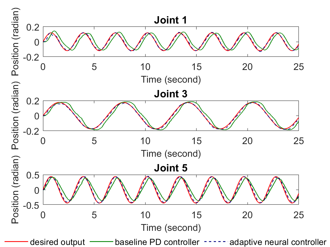
Figure 5 shows the representative results of joints 1, 3 and 5 for tracking an unseen sinusoidal joint position trajectory using the baseline PD controller in (4) and the adaptive controller in (7) and (9). The controller parameters are chosen as

$$(K_{1},K_{2})=(0.2,0.1),\,\,k=5,\,\,P=0.05$$

$$\Lambda=\mbox{diag}(3,6,3,20,10,10,10)$$

$$K_{s}=\mbox{diag}(0.1,0.01,0.01,0.1,0.01,0.01,0.01).$$

As a complete comparison, Table II lists the corresponding tracking errors in terms of $\ell_{2}$ and $\ell_{\infty}$ norms (using the error vectors at each sampling instant) for all 7 joints. From the figure and the table, it is clear that the adaptive neural controller outperforms the PD controller (in average over 60 % of improvement for all 7 joints).

Figure 5: Representative comparison of tracking performance with the baseline PD controller and the adaptive neural controller for sinusoidal joint position trajectories. See Table II for a complete comparison for all 7 joints.

TABLE II: $\ell_{2}$ and $\ell_{\infty}$ norm of tracking errors of the sinusoidal joint trajectories in Fig. 5 using the baseline PD controller and the neural adaptive controller.

	Baseline Controller	Adaptive Neural Controller
Joint	Tracking Error (rad)	Tracking Error (rad)
	$\ell_{2}\hskip 42.67912pt\ell_{\infty}$	$\ell_{2}\hskip 42.67912pt\ell_{\infty}$
1	2.7368       0.0885	0.5717       0.0473
2	1.8055       0.0715	0.5204       0.0311
3	2.0676       0.0706	0.5034       0.0275
4	2.6028       0.0955	0.4335       0.0290
5	7.4070       0.2534	2.3770       0.1064
6	5.9475       0.2274	1.6294       0.0803
7	4.7206       0.1873	2.2645       0.1278

V-B Experiment II: Comparative Study

We then conduct a comparative study to demonstrate the effectiveness of the regressor online learning scheme with a $\sim$0.6 kg payload attached to the robot gripper (the maximum payload of the gripper is around 5 pounds). We compare the tracking results of two systems with (system I) and without (system II) the regressor online learning by following the procedures as below:

Figure 6: Comparison of absolute tracking error using the developed adaptive controller with (blue curve) and without (red curve) the regressor online learning for tracking sinusoidal joint position trajectories.

• From $t=0\sim 25~{}s$, for both systems I and II, we use the controller in (7) but without the adaptation of $\hat{a}$ in (9). The value of $\hat{a}$ remains fixed and is from the trained network.

• At $t=25~{}s$, for both systems we attach the load to the robot gripper and implement the same controller as above.

• At $t=50~{}s$, we turn on the adaptive controller (with adaptation law in (9) activated) for both systems. We start collecting the input/output data of system I.

• For system I, we start implementing the regressor online update using the collected data every 25 seconds and the online updates are finished at $t=75~{}s$ and $t=100~{}s$, respectively. We find that the network weights converge after these two online updates.

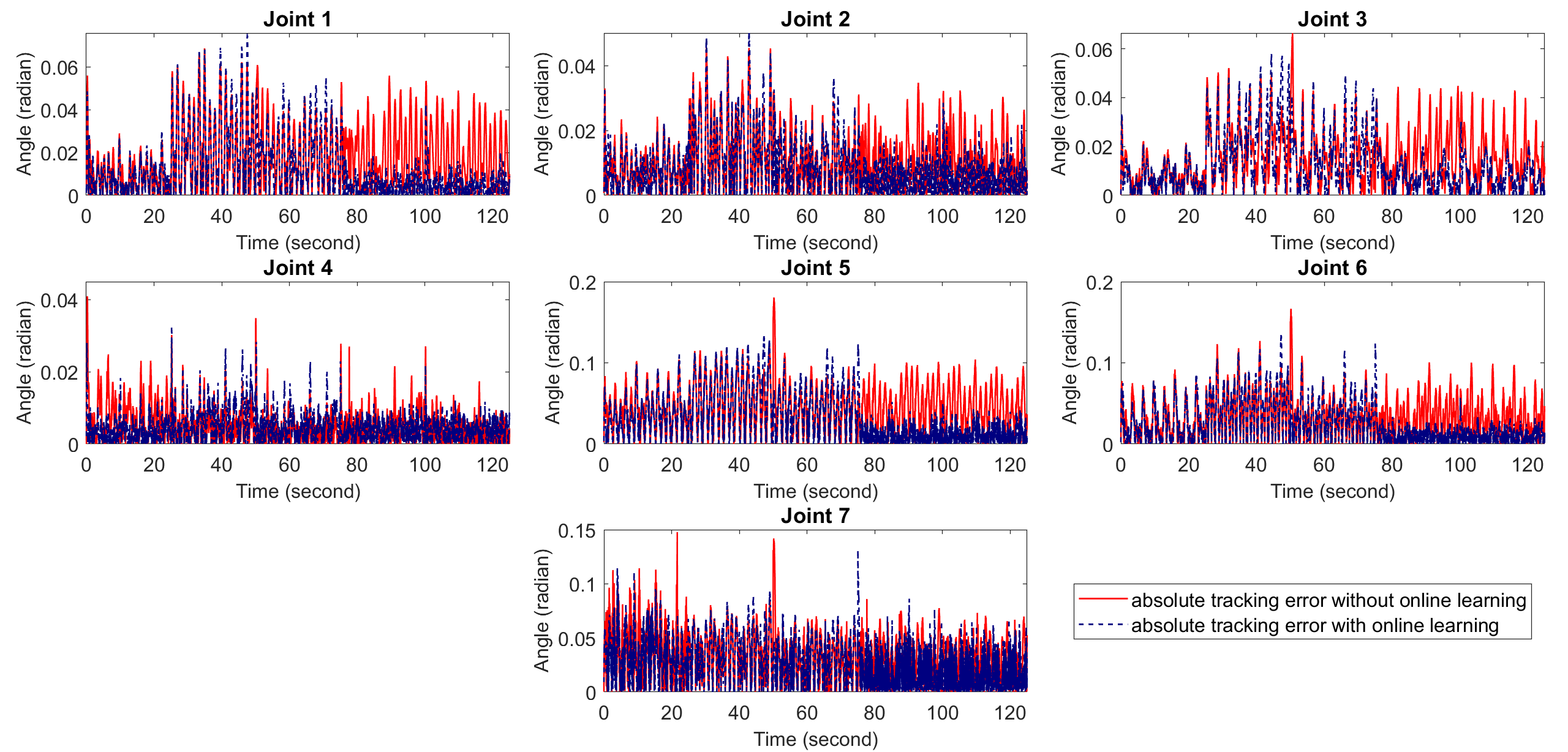
Figure 6 illustrates the comparison of the absolute tracking errors of two systems for the entire process. The error increases between $t=25~{}s\sim 50~{}s$ after attaching the load. After turning on the adaptive controller at $t=50~{}s$, the tracking errors of both systems decrease but the system I with online learning (dashed blue curve in Fig. 6) reduces further than system II (red curve in Fig. 6), starting from the first complete of online learning at $t=75~{}s$. Table III compares the Frobenius norm of tracking errors of all 7 joints at different stages for two systems. The table shows that two systems have similar tracking performance from $t=0\sim 75~{}s$ with the same condition. However, starting from $t=75~{}s$, system I presents a better tracking performance than system II due to the regressor online learning.

The comparison shows that the adaptive controller is able to compensate for the unknown load with the pure adaptation of the output layer weights. In addition, the online learning of regressor further reduces the tracking error with better model approximation.

TABLE III: Frobenius norm of tracking errors (in radian) of all 7 joints of the sinusoidal joint position trajectories in Fig. 6 using the neural adaptive controller with (system I) and without (system II) online learning of regressor.

	$[0,25]s$	$[25,50]s$	$[50,75]s$	$[75,100]s$	$[100,125]s$
I	2.1449	3.745	2.830	1.577	1.199
II	2.376	3.494	3.045	2.748	2.689

V-C Discussions

It remains an open problem to choose the proper update rate ratio between the regressor online learning and output layer weights adaptation. In the comparative experiment, we implement the regressor online update every 25 seconds whereas the output layer weights adapt at a rate around 100 Hz (thus a ratio of 2500:1). Potentially, the regressor online learning may be accelerated with a GPU.

In addition, the dynamics of a rigid-joint robot has a similar form to (2):

$$M(\theta)\ddot{\theta}+C(\theta,\dot{\theta})\dot{\theta}+G(\theta)=\tau,$$ (11)

where $\tau$ is the joint torque vector. By assuming the inner-loop torque control as

$$\tau=-K_{p}\cdot(\theta-\theta_{c})-K_{d}\dot{\theta}+G(\theta),$$ (12)

where $\theta_{c}$ is the commanded joint position. It follows

$$M(\theta)\ddot{\theta}+(C(\theta,\dot{\theta})+K_{d})\dot{\theta}+K_{p}\theta=K_{p}\theta_{c}.$$ (13)

By identifying the controller gains in (12) through collected data, we can relax the assumption of a scalar $K_{p}$, but use the identified $K_{p}$ to develop a similar neural adaptive controller.

VI Conclusions and Future Work

In this work, we proposed a novel neural adaptive controller that demonstrates asymptotically trajectory tracking for a flexible-joint robot with unknown dynamics. Initialized by a simple offline training, the proposed neural network which is composed of a regressor and an output layer, emulates the linear-in-parameter form of the robot dynamics. The regressor network updates online at a slower rate compared to the adaptation of the output layer weights. By simulation and experiments, the proposed control framework improves the trajectory tracking performance of the system. With the regressor online learning, the tracking performance of the adaptive controller is further improved.

Future work includes the exploration of choosing a proper update ratio between the regressor network and the output layer. It is also interesting to test the proposed control framework with rigid-joint robot manipulators as discussed above. Finally, we plan to compare the proposed approach with other neural adaptive controllers.

References

- [1] Z. Qu and D. M. Dawson, Robust tracking control of robot manipulators. IEEE press, 1995.
- [2] J.-J. E. Slotine and W. Li, “On the adaptive control of robot manipulators,” The international journal of robotics research, vol. 6, no. 3, pp. 49–59, 1987.
- [3] M. Spong, K. Khorasani, and P. Kokotovic, “An integral manifold approach to the feedback control of flexible joint robots,” IEEE Journal on Robotics and Automation, vol. 3, no. 4, pp. 291–300, August 1987.
- [4] S. Arimoto, “Learning control theory for robotic motion,” International Journal of Adaptive Control and Signal Processing, vol. 4, no. 6, pp. 543–564, 1990.
- [5] H. Miyamoto, M. Kawato, T. Setoyama, and R. Suzuki, “Feedback-error-learning neural network for trajectory control of a robotic manipulator,” Neural Networks, vol. 1, no. 3, pp. 251 – 265, 1988.
- [6] B. Brogliato, R. Ortega, and R. Lozano, “Global tracking controllers for flexible-joint manipulators: a comparative study,” Automatica, vol. 31, no. 7, pp. 941–956, 1995.
- [7] D. Wang, “A simple iterative learning controller for manipulators with flexible joints,” Automatica, vol. 31, no. 9, pp. 1341–1344, 1995.
- [8] T. H. Lee and C. J. Harris, Adaptive neural network control of robotic manipulators. World Scientific, 1998, vol. 19.
- [9] C. Lin, “Nonsingular terminal sliding mode control of robot manipulators using fuzzy wavelet networks,” IEEE Transactions on Fuzzy Systems, vol. 14, no. 6, pp. 849–859, Dec 2006.
- [10] C. Williams, S. Klanke, S. Vijayakumar, and K. M. Chai, “Multi-task gaussian process learning of robot inverse dynamics,” in Advances in Neural Information Processing Systems 21, D. Koller, D. Schuurmans, Y. Bengio, and L. Bottou, Eds. Curran Associates, Inc., 2009, pp. 265–272.
- [11] H. Ho, Y. Wong, and A. Rad, “Robust fuzzy tracking control for robotic manipulators,” Simulation Modelling Practice and Theory, vol. 15, no. 7, pp. 801 – 816, 2007.
- [12] Y. Jiang, C. Yang, J. Na, G. Li, Y. Li, and J. Zhong, “A brief review of neural networks based learning and control and their applications for robots,” Complexity, vol. 2017, pp. 1–14, 10 2017.
- [13] J. H. Perez-Cruz, I. Chairez, J. de Jesus Rubio, and J. Pacheco, “Identification and control of class of non-linear systems with non-symmetric deadzone using recurrent neural networks,” IET Control Theory Applications, vol. 8, no. 3, pp. 183–192, Feb 2014.
- [14] H. A. Talebi, R. V. Patel, and K. Khorasani, “Inverse dynamics control of flexible-link manipulators using neural networks,” in Proceedings. 1998 IEEE International Conference on Robotics and Automation (Cat. No.98CH36146), vol. 1, May 1998, pp. 806–811 vol.1.
- [15] S. Chen and J. T. Wen, “Neural-Learning Trajectory Tracking Control of Flexible-Joint Robot Manipulators with Unknown Dynamics,” in 2019 IEEE/RSJ International Conference on Intelligent Robots and Systems (IROS), Nov 2019.
- [16] S. Chen and J. T. Wen, “Industrial Robot Trajectory Tracking Using Multi-Layer Neural Networks Trained by Iterative Learning Control,” arXiv e-prints, 2019.
- [17] K. S. Narendra and K. Parthasarathy, “Identification and control of dynamical systems using neural networks,” IEEE Transactions on Neural Networks, vol. 1, no. 1, pp. 4–27, March 1990.
- [18] L. Jin, S. Li, J. Yu, and J. He, “Robot manipulator control using neural networks: A survey,” Neurocomputing, vol. 285, pp. 23 – 34, 2018.
- [19] S. J. Yoo, J. B. Park, and Y. H. Choi, “Adaptive output feedback control of flexible-joint robots using neural networks: Dynamic surface design approach,” IEEE Transactions on Neural Networks, vol. 19, no. 10, pp. 1712–1726, Oct 2008.
- [20] M. Wang, H. Ye, and Z. Chen, “Neural learning control of flexible joint manipulator with predefined tracking performance and application to baxter robot,” Complexity, vol. 2017, pp. 7 683 785:1–7 683 785:14, 2017.
- [21] W. He, Z. Yan, Y. Sun, Y. Ou, and C. Sun, “Neural-learning-based control for a constrained robotic manipulator with flexible joints,” IEEE Transactions on Neural Networks and Learning Systems, vol. 29, no. 12, pp. 5993–6003, Dec 2018.
- [22] C. Yang, X. Wang, L. Cheng, and H. Ma, “Neural-learning-based telerobot control with guaranteed performance,” IEEE Transactions on Cybernetics, vol. 47, no. 10, pp. 3148–3159, Oct 2017.
- [23] I. Ranatunga, S. Cremer, F. L. Lewis, and D. O. Popa, “Neuroadaptive control for safe robots in human environments: A case study,” in 2015 IEEE International Conference on Automation Science and Engineering (CASE), Aug 2015, pp. 322–327.
- [24] F. L. Lewis, A. Yesildirek, and K. Liu, “Multilayer neural-net robot controller with guaranteed tracking performance,” IEEE Transactions on Neural Networks, vol. 7, no. 2, pp. 388–399, March 1996.
- [25] G. Shi, X. Shi, M. O’Connell, R. Yu, K. Azizzadenesheli, A. Anandkumar, Y. Yue, and S.-J. Chung, “Neural Lander: Stable Drone Landing Control using Learned Dynamics,” arXiv e-prints, p. arXiv:1811.08027, Nov 2018.
- [26] A. Noormohammadi-Asl, M. Saffari, and M. Teshnehlab, “Neural control of mobile robot motion based on feedback error learning and mimetic structure,” in Electrical Engineering (ICEE), Iranian Conference on, May 2018, pp. 778–783.
- [27] J. Umlauft and S. Hirche, “Feedback linearization based on gaussian processes with event-triggered online learning,” IEEE Transactions on Automatic Control, pp. 1–1, 2019.