Evaluating Abstract Asynchronous Schwarz solvers.

Abstract

With the commencement of the exascale computing era, we realize that the majority of the leadership supercomputers are heterogeneous and massively parallel even on a single node with multiple co-processors such as GPU’s and multiple cores on each node. For example, ORNL’s Summit accumulates six NVIDIA Tesla V100’s and 42 core IBM Power9’s on each node. Synchronizing across all these compute resources in a single node or even across multiple nodes is prohibitively expensive. Hence it is necessary to develop and study asynchronous algorithms that circumvent this issue of bulk-synchronous computing for massive parallelism. In this study, we examine the asynchronous version of the abstract Restricted Additive Schwarz method as a solver where we do not explicitly synchronize, but allow for communication of the data between the sub-domains to be completely asynchronous thereby removing the bulk synchronous nature of the algorithm.

We accomplish this by using the onesided RMA functions of the MPI standard. We study the benefits of using such an asynchronous solver over its synchronous counterpart on both multi-core architectures and on multiple GPU’s. We also study the communication patterns and local solvers and their effect on the global solver. Finally, we show that this concept can render attractive runtime benefits over the synchronous counterparts.

Keywords Asynchronous solvers; Parallel Numerical Linear Algebra;Abstract Schwarz methods;Exascale; Multicore Processors, GPUs

1 Introduction

As of today, many of the leadership HPC systems draw a significant portion of their compute power from accelerators like GPUs. For example, each node of the Summit supercomputer (Oak Ridge National Laboratory, US) features 6 NVIDIA Volta V100 accelerators, for a total theoretical peak performance of 40 TFlop/s. In contrast, the CPU has a theoretical peak performance of 1 TFlop/s. Accumulating a significant portion of the compute power in highly-parallel accelerators amplifies the impact of global synchronization points, and there is an urgent need to move beyond the Bulk-Synchronous Programming Model (BSP). This is reflected in the US Department of Energy listing the removal of synchronization bottlenecks as one of the programming challenges for the exascale era [1].

In consequence, new algorithms should be designed as asynchronous, fault tolerant, accelerator friendly and agile in terms of adapting to load imbalance. From the perspective of linear solvers, there are two possible approaches. The first approach features improving the load balancing of the algorithms and moving to more asynchronous programming techniques. The second approach is based on the use of asynchronous iterative methods. While the first approach provides some performance improvements, it may fail for some algorithms such as the traditional iterative methods that compute in a lock-step fashion and have synchronization points boiled into the algorithm. Asynchronous iterative methods, on the other hand, do not operate in a lock-step fashion, but instead allow for using the available data without explicitly synchronizing all the processes at every iteration. This removes the bulk-synchronous character of the algorithm, and allows to move to a more asynchronous model where each process trades the global synchronization against the price of possibly computing on old data. In an abstract view, asynchronous iterative methods trade computation cost for synchronization cost.

There has been significant research on the characteristics and convergence of asynchronous methods ([2, 3, 4] and references therein), and it has been demonstrated that asynchronous methods can potentially converge faster than their synchronous counterparts (from a time-to-solution perspective). Nonetheless, production-ready implementations on HPC architectures and comprehensive studies of these are a scarce resource, in particular in the context of machines featuring accelerators such as the Summit HPC system. In this paper, we implement the abstract Restricted Additive Schwarz algorithm as a solver for linear systems. For architectures featuring multiple GPUs in multiple nodes, we show that the asynchronous algorithm is faster than its synchronous counterpart. Up to our knowledge, this is novel work, and we hence highlight the following novel contributions:

• We present an open source implementation of an asynchronous Restricted Additive Schwarz algorithm for multi-node systems featuring accelerators.

• We provide a software which can be used as a testbed for synchronous and asynchronous methods. The software can be used on a wide range of hardware architectures, features support for both direct and iterative local solves, supports one-sided and two-sided MPI communication, and supports both centralized and decentralized convergence detection.

• We show that asynchronous iterative methods can provide significant performance improvements over synchronous methods on modern GPU-centric HPC systems.

• We study the effect of different partitioning schemes, overlap size, two-sided vs one-sided MPI communication, and centralized vs decentralized convergence detection.

In Section Background we first provide some background on the Schwarz methods, asynchronous iterative methods, and the different convergence detection schemes. In Section Implementation, we describe the new algorithm framework that we develop with its capabilities, and the settings we use in the experimental evaluation that we present in Section Experimental Assessment. We conclude in Section Conclusion and Future work.

2 Background

2.1 Schwarz methods.

Schwarz methods are a class of domain decomposition methods that were initially used in [5] as a theoretical tool to show the existence of solutions for the Laplace equation through the alternating method. Since then, many variants of the method have found their use as iterative methods, e.g,  [6, 7, 8, 9, 10], and as preconditioners, e.g,  [11, 12].

We aim to solve linear systems of the form

$$Ax=b.$$ (1)

The general idea of domain decomposition (DD) solvers is to decompose the domain into distinct subsets so that the local solution for each of those subdomains can be computed in parallel. To facilitate this and account for the decomposition, they need to exchange data from each other to reach a global solution.

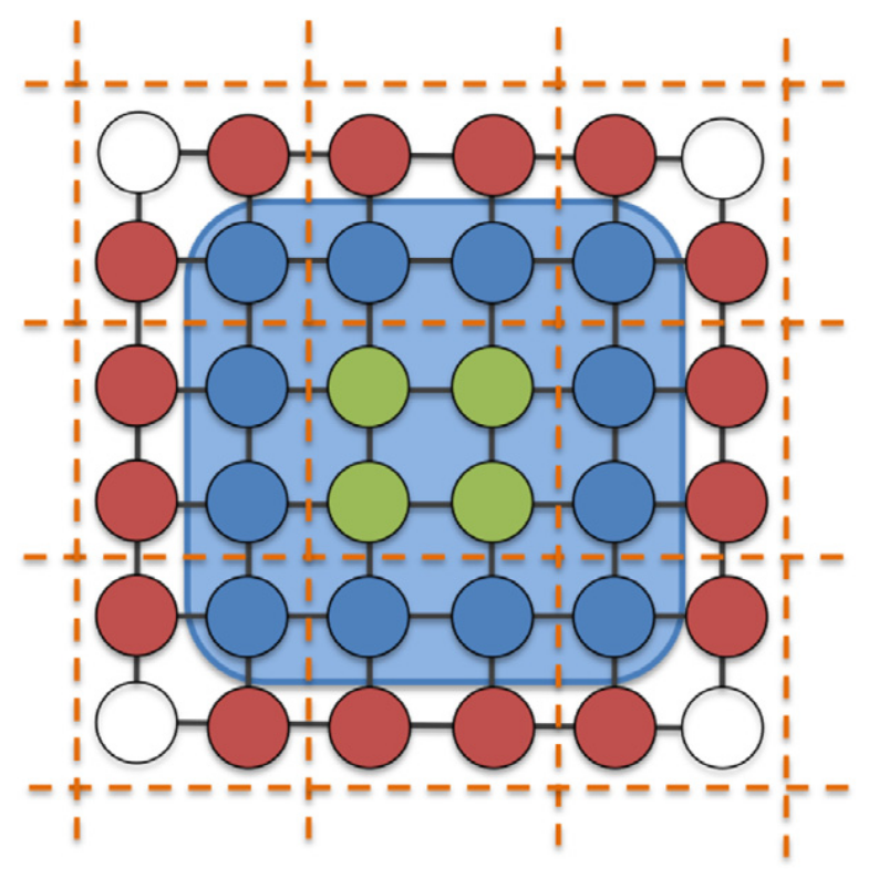
Figure 1: Decomposed 2-D grid with partitioning and overlap. From [13]

Consider a two dimensional grid as shown in Figure 1. The dashed orange lines show the partitioning of the mesh into 3x3 subdomains. The interior of one subdomain is shown in green. If every point is part of only one subdomain, the DD method is called a non-overlapping decomposition. If, for example, the subdomain owning the green points includes also the blue points as variables in the solution of the local problem, then the DD method is said to be an overlapping domain decomposition solver, in this case with overlap $\gamma=1$. This is the definition of overlap we use throughout this paper. In this setting, the points marked red are the external interface points through which the information is exchanged.

In an overlapping additive Schwarz method, the values for the grid points in the overlap are computed by several subdomains, and to form a unique global solution, the different locally-computed values need to be weighted ([14, 15]). With a modification proposed by [16], the grid points in the overlap are still considered as variables when computing the local solution, but discarded afterwards. This modification is called the Restricted Additive Schwarz (RAS) and combines the advantage of converging faster [16] with the advantage of removing any need for weighting overlap solutions and therewith allowing for collision-free implementation on parallel computing architectures.

In synchronous Schwarz solvers, the iterations are realized in a lock-step fashion: the domain is decomposed into subdomains as presented, local solves are performed in parallel, each subdomain sends the required data to its “neighbors,” and all the subdomains wait until data has been received from their neighbors. Global convergence is achieved when the global solution – computed after all subdomains solved the local problems – satisfies a pre-defined convergence criterion.

Asynchronous Schwarz solvers on the other hand remove the explicit synchronizations separating the iterations ([17, 18]). Instead, each subdomain proceeds by solving the local problem using the latest data it received from neighboring subdomains. This has several critical implications ([19]): 1) there is no longer a concept of “global iterations” as the distinct subdomains can differ in how many local solves they completed; 2) local solves can potentially re-compute the same solution in case no new data was received; 3) the asynchronous Schwarz convergence and performance is not reproducible as – theoretically – each algorithm execution results in a different subdomain update order and communication pattern; and 4) the lack of global synchronization points requires alternative strategies for detecting convergence of the algorithm. Convergence for the asynchronous Schwarz methods and their variants have been shown, for example in [20, 21, 19].

2.2 Convergence detection

Convergence detection in an asynchronous algorithms lacking global synchronization points is a challenging endeavor. There exists a variety of strategies to detect convergence of a truly asynchronous algorithm running in a distributed framework, see, e.g., [22], [23], and [24] for innovative ideas.

In general, the convergence detection strategies can be classified into two main categories: centralized and de-centralized convergence detection algorithms. In centralized termination detection, like the one presented in [13], a root/leaf paradigm is used, where, each of the leaf processes reports the convergence status to the root, and the root conversely sends a termination signal if all of its leaf processes have converged. In the case of decentralized convergence detection like presented in [25], there is no such root/leaf paradigm, but each subdomain communicates its convergence status to its neighbors and a subdomain propagates global convergence of its solution once it received convergence from all of its neighbors.

3 Implementation

The testbed framework we develop for asynchronous iterative methods is written in C++ and features a modern C++ design. The framework is intended to be customizable and extensible, and features multiple options which can be tweaked or easily added to explore the benefits of various techniques and concepts in the context of asynchronous iterative methods.

Core of the framework is the algorithm detailed in Section Core Algorithm. This algorithm is generic enough to be reused for other asynchronous iterative methods since it only calls different sub-components, which are the Initialize interface detailed in Section Initialization and setup and the Solve interface detailed in Section Solving the local problems. The Communicate interface, used in both the Initialize and the Solve step, supports MPI one-sided and two-sided communication and is detailed in Section Communication.

The framework we develop interacts with multiple external tools to provide specific functionalities, among which are Metis ([26]) for partitioning, deal.ii ([27]) for generating problems, and the Ginkgo [28] framework for local solvers, generic data management and certain execution management features as presented in Section The Ginkgo framework.

3.1 Core Algorithm

Algorithm 1 shows the steps involved in the RAS solve. The initialization step handles the setup and initialization of the solver, while the solve step handles the local solves, communication, the convergence detection, and the termination of the solver. The timings and performance data we report in Section Experimental Assessment account only for the solve step as the initialization and setup is a constant, non-repeating part of the RAS solver.

1:procedure iterative_solution($A,x,b$)

2:     procedure initialization_and_setup

3:         Partition matrix $\triangleright$ Regular / objective based

4:         Distribute data

5:         Initialize data      

6:     procedure solve

7:         while $iter<max\_iter$ or until convergence do

8:              Locally solve the matrix $\triangleright$ Iterative / Direct

9:              Exchange boundary information

10:              Update boundary information

11:              Check for Convergence $\triangleright$ Centralized/Decentralized          

12:         Gather the final solution vector      

Algorithm 1 Schwarz Iterative solver

3.2 Initialization and setup

The initialization and setup step consists of three main parts: 1. the generation and partitioning of the global system matrix; 2. the distribution/generation of the local subdomain matrices and right hand sides; and 3. the setup of the communication – which is detailed in Section Communication as it is a separate component impacting both the initialization and the solve characteristics.

3.2.1 Partitioning

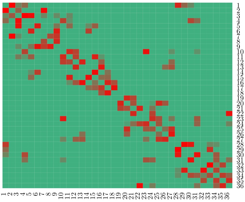
(a) Metis

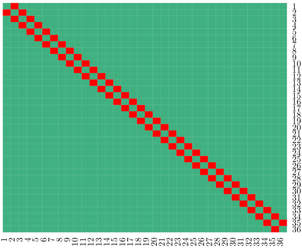
(b) Regular 1D

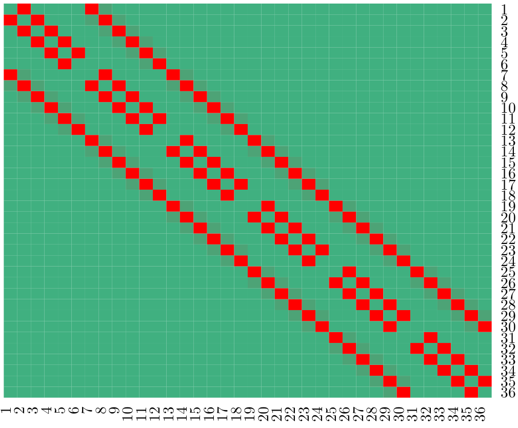
(c) Regular 2D

Figure 2: Communication patterns resulting from different partitioning schemes. Subdomain IDs are indicated on the bottom and the right of the communication patterns.

The framework we develop currently supports three partitioning schemes. Figure 2 shows the communication patterns that arise for the three partitioning schemes as heatmaps for a 2D Laplace problem discretized using a 5 point stencil. The communication volume each process receives from its neighbor is governed by the partitioning scheme. The color-fill in the cells indicate the amount of communication between the subdomains with the row column pair. Green indicates no communication and red indicates a significant data volume being exchanged.

In a one-dimensional regular1d partitioning, each subdomain has at most two neighbors and a very regular communication pattern. At the same time, it is not very efficient as the information propagation is slow: For $N$ subdomains, the rate of information propagation, defined here as the amount of solver iterations needed for data exchange between the two farthest subdomains, is $N-1$.

In a two-dimensional regular2d partitioning, each subdomain can have at most 4 neighbors. This allows for faster information propagation at the cost of increased communication compared to the regular1d scheme.

On the other hand, using the metis partitioning scheme, each subdomain can have multiple neighbors, and therefore the "farthest distance" can be significantly smaller.

3.2.2 Local subdomain matrices

The partitioning scheme assigns each grid point to a subdomain (or multiple, if the grid point is part of the overlap). This information is used to assemble the local subdomain matrix and an interface matrix that is used to communicate between the different subdomains using a SpMV formulation.

We store all the matrices in the CSR format, which is a popular matrix format for handling sparse matrices, and which has been shown to perform well for a given generic matrix. We note that as we use the Ginkgo library, we are not restricted to this particular format since we can use any other format supported by Ginkgo (e.g. COO, ELL, Hybrid) [29].

3.3 Solving the local problems

3.3.1 Local solution

Each subdomain has its own local matrix and right hand side, and can thus independently solve the local problem. The local solution can be computed with a direct solver (computing a LU/Cholesky factorization of the local system once and solving triangular systems in each iteration), or using an iterative solver such as CG, GMRES, BiCGSTAB, etc.

In the experimental evaluation, we focus on direct local solves and use the Cholesky factorization available in the CHOLMOD library (part of the SuiteSparse package) [30]. The arising triangular systems are handled with Ginkgo’s triangular solve – which in turn interfaces to NVIDIA’s cuSPARSE library [31]. Using CUDA version 10.1, the cusparse_csrsm2 sparse triangular solve routine is based on the level-set strategy and capable of handling multiple right hand sides.

3.3.2 Convergence detection

The framework we develop supports two convergence detection strategies: a centralized (tree-based) convergence detection mechanism and a decentralized strategy.

Centralized, tree based: This implementation follows the idea presented in [13] in which the children processes detect local convergence and pass this result to their parent processes. Once the main root has received such a message, it broadcasts a termination to all its children to terminate the iterative process.

The local convergence criterion for each of the subdomains is

$$||\tilde{r}_{p}||^{2}_{2}<\tau^{2}||\tilde{b}_{p}||^{2}_{2},$$ (2)

where $\tilde{r}_{p}$ is the local residual vector with the values of the subdomain $p$ (including those in the overlap), $\tau$ is the global solver tolerance, and $\tilde{b}_{p}$ is the local right hand side. The global convergence criterion is

$$||r||<\tau||b||$$

where $r$ is the global residual vector and $b$ is the global right hand side. Once all the subdomains have satisfied their local convergence criteria, we additionally verify that the global convergence criterion is satisfied post termination.

Decentralized, leader based: This implementation follows the idea presented in [25]. In this detection algorithm, each subdomain considers the number of neighbors that have sent a local convergence message. Once all neighbors have confirmed convergence, the subdomain broadcasts the global convergence flag to all its neighbors, which in turn broadcast it to their neighbors and so on. The local convergence criterion is the same as in (2) and, as in the previous algorithm, the processes first detect their local convergence status and propagate this to their neighbors.

3.4 Communication

The communication class in our framework handles the communication between the subdomains. It has two main functionalities. First is the setup and allocation of all the MPI windows and the communication buffers that handle the communication between the subdomains. This is shared with the Initialization class. Second is the detection of convergence and termination of the solver. This is shared with the Solver class. We now explain the setup for the two cases:

Synchronous Schwarz setup: With the synchronous version, each step in the solve procedure in Algorithm 1 is performed in a lock-step fashion. We associate each subdomain to one MPI rank. A subdomain here refers to the computational unit that performs a local solve and communicates the required data to its “neighbors”. Currently, the subdomains in one RAS solve are restricted to either only GPUs or only CPUs.

We use MPI point to point communication to communicate between the different subdomains. We use the CUDA-aware MPI to directly transfer the buffers between GPUs of different subdomains instead of intermediately staging them on the CPU. This allows for faster communication as the latencies from the CPU side are hidden (particularly for GPUs attached to the same socket and communicating via the CUDA NVLINK technology [32]). We use the non-blocking point to point functions MPI_Isend and MPI_Irecv to send and receive data between the subdomains. Before sending, the data is first packed and after receiving the target subdomain unpacks it. An MPI_Wait is called by each subdomain to wait for the MPI_Isend from its neighboring processes. This results in explicit synchronization points separating the Schwarz iterations.

Asynchronous Schwarz setup: In the asynchronous version, each step in the solve procedure in Algorithm 1 is executed without synchronizing with neighbors. The MPI-2 standard ([33]) introduced the Remote Memory Access (RMA) functions that allow remote MPI ranks to access dedicated buffers without explicit synchronization. Each process can “put” its data into the buffer of its neighbors through a “window” using the RMA function MPI_Put. To make sure that the operations are completed, a “flush” is called on the windows. Avoiding global synchronization points makes this algorithm truly asynchronous in terms of the communication.

3.5 The Ginkgo framework

The Ginkgo numerical linear algebra library is a node-level high performance sparse linear algebra library featuring high performance kernels for different back-ends such as multicore (OpenMP), AMD GPUs (HIP) and Nvidia GPUs (CUDA). Ginkgo provides the user with simple and powerful linear operator abstraction to interface various solvers, preconditioners, and matrix operations. In the experimental analysis, we use Ginkgo objects for all arrays, matrices, and vectors. This enables us to leverage Ginkgo’s executor concept – it allows to easily move from one hardware architecture to another without code changes except for choosing another execution space. As we are focusing on the architecture of the Summit supercomputer, we can run our Schwarz framework on the V100 GPUs using Ginkgo’s CUDA executor.

4 Experimental Assessment

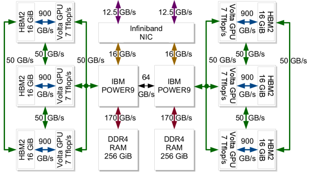
Figure 3: On-node hardware connectivity diagram for the Summit supercomputer at Oak Ridge National Laboratory based on IBM POWER9 processor and NVIDIA Volta GPU accelerators.

4.1 Hardware and software setup

For the experimental analysis we focus on the 2D Laplace problem discretized using a 5 point stencil, $\mathcal{S}=\{-1,-1,4,-1,-1\}$ with offsets $\{-N,-1,0,1,N\}$ and $N$ being the number of grid points in each discretization direction. The resulting linear system is very regular, therewith promoting good load balance and making it particularly difficult for asynchronous methods to outperform synchronized counterparts.We use a random RHS, and define the convergence of the RAS solver once the relative residual norm drops below $1e-7$. We would also like to mention that the RAS solver is capable of solving a generic linear system when coupled with a generic local solver such as LU/GMRES.

The benchmark runs are conducted on the Summit supercomputer at the Oak Ridge National Lab. Each node composes of two IBM Power 9 CPUs and 6 NVIDIA Tesla V100 GPUs. The 3 GPUs connected to the same socket are directly connected to each other via a NVLINK brick with a 50GB/s bi-directional bandwidth, see Figure 3 [34]. Each V100 features 16GB of High Bandwidth Memory (HBM2). In total, the Summit supercomputer contains more than 4,600 nodes of this kind. The nodes are connected via a dual-rail EDR InfiniBand network (non-blocking fat tree) providing a bandwidth of 23GB/s. Hence, in the scaling analysis, we need to consider the different bandwidth capabilities. The fastest communication between two GPU’s is through the direct NVLINK (50GB/s) that connects GPU’s of the same node. The second fastest communication is the off-socket on-node , but still on node: NVLINK (50GB/s) – Inter-socket (64GB/s) – NVLINK (50GB/s) path. The slowest communication is between GPU attached to different nodes, which requires going through the “slow” Interconnect (23GB/s).

This paper’s codebase uses Ginkgo as a central building block for the RAS solver. Overall, local on-node (on-GPU) operations use Ginkgo functionality, while the communication is handled via MPI. As we perform our experiments on the Summit system, we use the IBM Spectrum MPI library (a flavor of OpenMPI). Related work [13] analyzes the impact of using different MPI implementations including the performance of the one-sided RMA functions.

Investigating asynchronous methods like the asynchronous RAS solver is challenging for several reasons. First, due to the non-deterministic behavior, we are generally unable to predict or reproduce results and effects. At best, we can report statistical data and draw weak assumptions. In consequence, all data we present for the asynchronous RAS in this paper is averaged over 10 runs. Second, in asynchronous iterative methods, the concept of iterations does no longer exist. Removing explicit synchronization points it is possible that some solver parts (i.e. subdomains) have already completed a high number of local solves while other parts did not yet complete a single local solve. To reflect this challenge, we base all performance data we report on the asynchronous RAS on the time-to-solution. This is the total time until global convergence is detected – which brings us to a third challenge: without global synchronization points, it is difficult to detect global convergence. The framework we develop supports both centralized and decentralized convergence detection, and while we analyze the performance effect of these strategies at the end of this section, we use decentralized convergence as default setting.

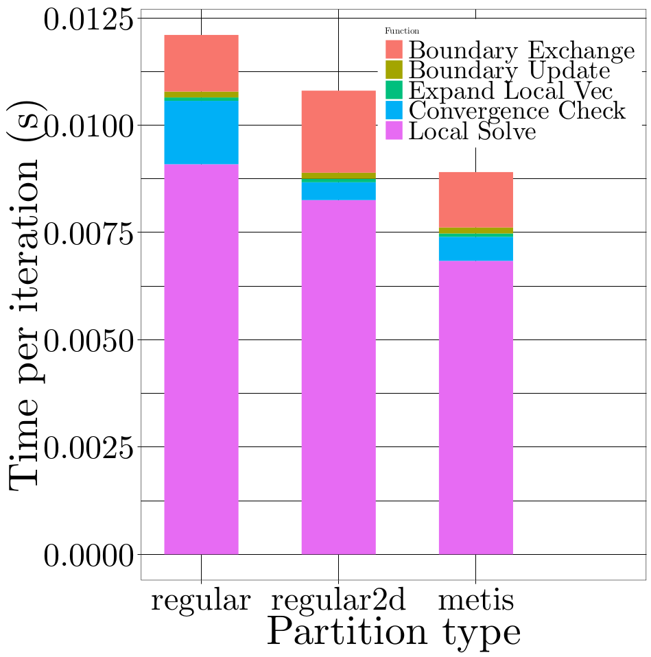
(a) Runtime breakdown for the averaged subdomain update

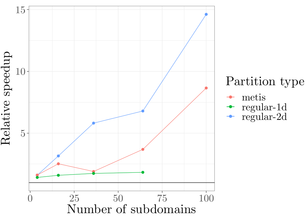
(b) Speedup - Asynchronous vs Synchronous

Figure 4: Comparing the different partitioning strategies. (a) shows the time spent in the different functions (sync), and (b) shows the speedup of the asynchronous version over the synchronous version.

4.2 Comparing partitioning strategies

Figure 4(a) visualizes the runtime needed for one synchronous RAS iteration using two-sided MPI communication averaged over all the subdomains (problem with 262144 unknowns divided into 4 subdomains). Different partitioning strategies are considered. Partitioning affects the solution in two ways: On the one hand, it affects the fill-in governed by the factorization of the local subdomain matrices. regular-2d and metis are better at minimizing the fill-in of the resulting local matrices when distributing the rows to the subdomains. Hence, we expect that the local solve is cheaper when using regular-2d and metis. On the other hand, it dictates the communication volume between the subdomains. metis is better in minimizing the edge cut of the adjacency matrix, and the communication time is reduced compared to regular-2d.

For a weak scaling analysis, we now fix the local problem size to 4096 elements per subdomain, and assess the time-to-solution speedup of the synchronous RAS solver using regular-2d and metis over regular-1d for increasing subdomain counts.

In Figure 4(b) we investigate the effect of abandoning the synchronization points in the RAS solver. Again, the speedup is based on the time-to-solution and the asynchronous versions of the partitioning methods are compared to their synchronous counterparts. The number of elements per subdomain is set to 4096 and we increase the number of subdomains from 4 to 100. The regular-1d partitioning does not scale for a large number of processes. We observe that as we increase the number of subdomains, the asynchronous version outperforms the synchronous version for all partitioning methods even reaching a maximum speedup of about 15$\times$ for a large number of subdomains for the regular-2d partitioner. The performance of the regular-2d partitioner is on average 1.3 $\times$ slower than when metis partitioner is used for the synchronous version. We would like to compare the performance of our asynchronous solver with the best parameters for the synchronous version, and given the fact that metis is a generic partitioner (applicable to any generic matrix), we choose to run all our experiments with the metis partitioner.

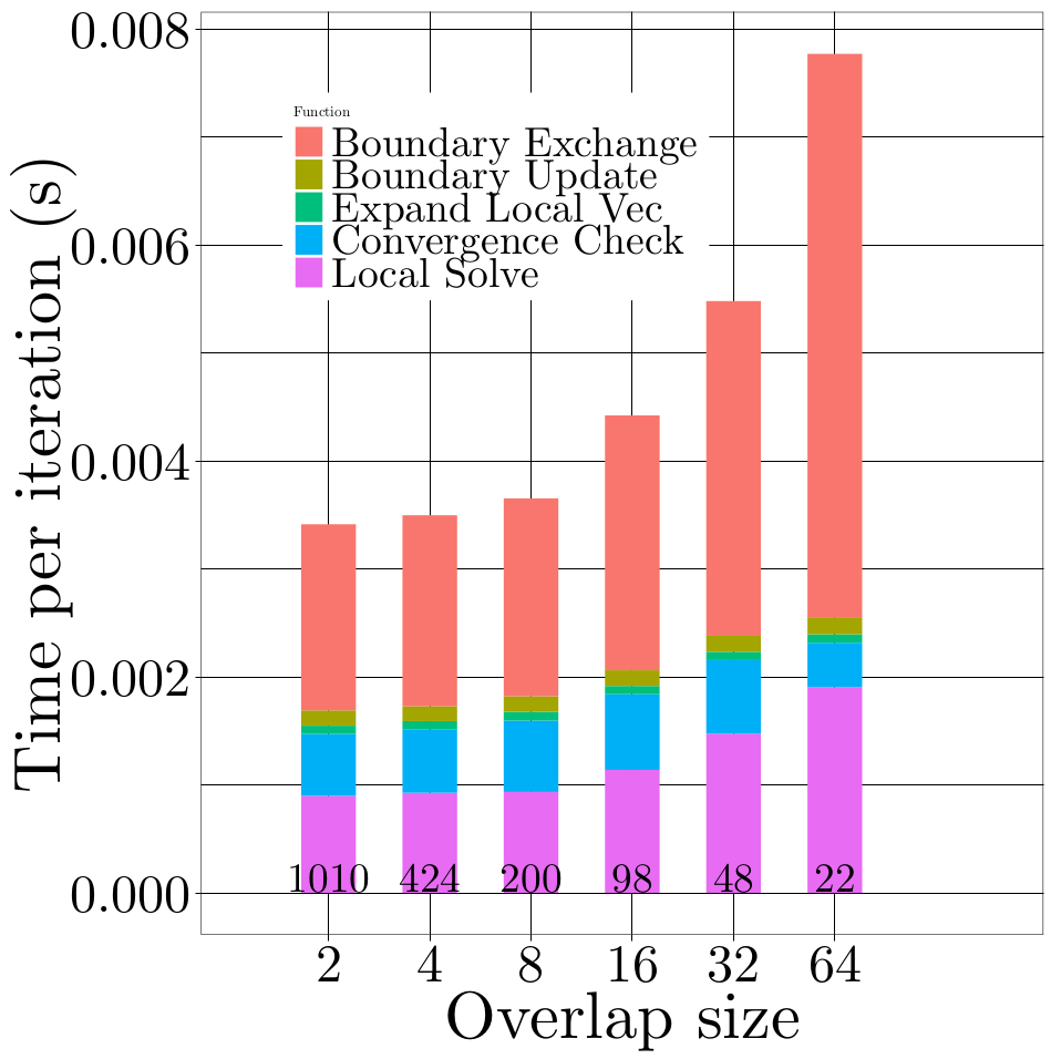
(a) Runtime breakdown for the averaged subdomain update & subdomain update count

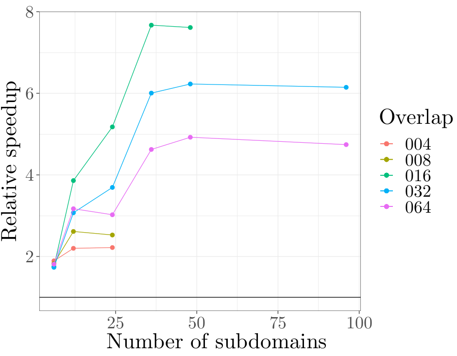
(b) Speedup - Asynchronous vs Synchronous

Figure 5: Comparing the different overlaps between the subdomains. (a) shows the time spent in different functions (synchronous version), (b) shows the speedup of the asynchronous version over the synchronous version.

4.3 Comparing different overlaps

Figure 5(a) shows for different overlap sizes the time spent in the different components of a single (synchronized) RAS iteration and the total number of RAS iterations needed for convergence. The global problem of size 16384 is decomposed into 6 subdomains, and only the overlap is varied. All timings are averaged over the 6 subdomains. A minimal overlap of 2 elements is required for the RAS method to converge, but a minimal overlap is inefficient as the information propagation is slow, which results in the RAS solver needing over 1000 iterations to converge. The local problem size increases with the overlap, increasing the cost of the local solves. The time for "Boundary Exchange" also increases with the overlap as more data has to be communicated. At the same time, the larger overlaps enabling the faster information propagation promotes much faster convergence, i.e. reduce the number of needed RAS iterations. The optimal overlap has to balance between these aspects and depends on the problem characteristics, the partitioning scheme, and the ratio between compute power and memory bandwidth of the used architecture. The asynchronous solver benefits from having a high overlap because higher overlaps reduce the message cost and do not have the synchronizations that adversely affect the synchronous version. This is also seen from Figure 5(b), where we compare the speedup for same overlap size of the asynchronous version against the synchronous version for varying problem size. The time to converge for the lower overlap values, namely “4” and “8” for especially the synchronous version is high and excluded from this graph. The asynchronous version can perform much better than the synchronous version when using an overlap of size “16” as most of the communication time can be hidden.

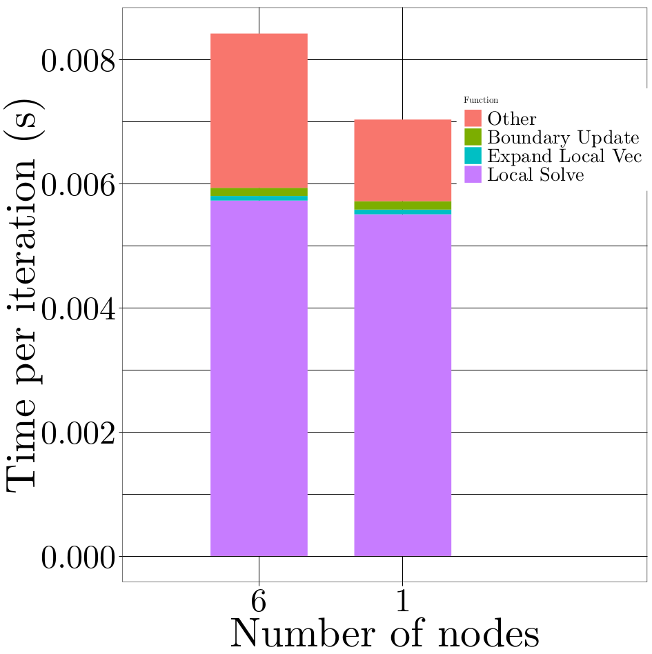
(a) Runtime breakdown for the averaged subdomain update (Asynchronous)

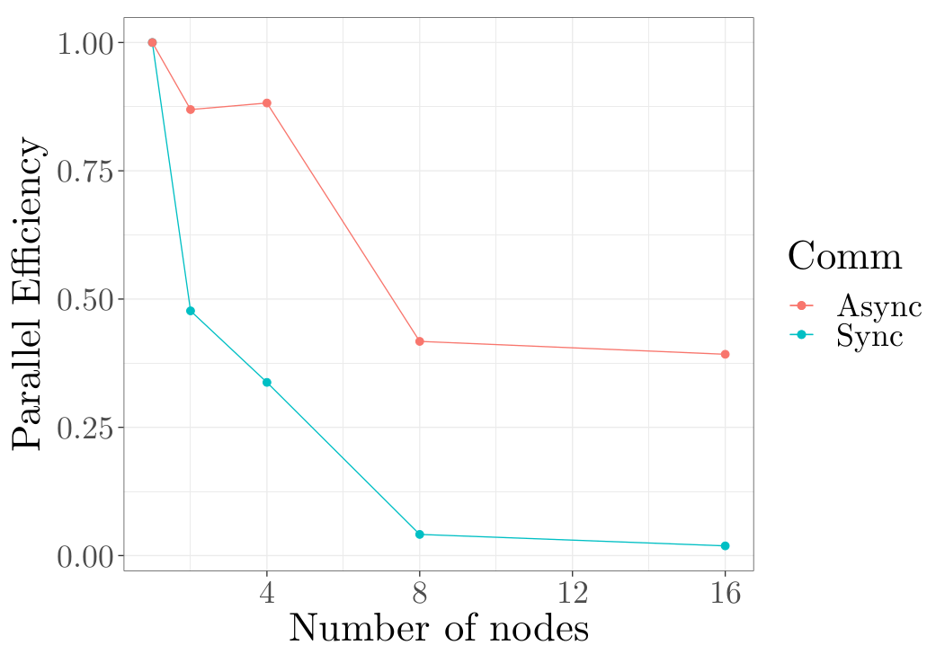
(b) Scaling Efficiency

Figure 6: Comparing scaling on increasing number of nodes. (a) shows the time spent in different functions, (b) shows the parallel scaling efficiency

4.4 Scalability study

Before investigating the scalability of the synchronous and asynchronous RAS solver, we study the effect of the internode vs NVLINK bandwidths. In the asynchronous RAS, we can not isolate the communication operations, but we can measure the overall time-to-solution and the time each subdomain spends on solving the local problem. Figure 6(a) visualizes the time spent in different routines when using 6 subdomains, either executed in 6 GPUs attached to the same node, or in 6 GPUs attached to distinct nodes. The averaged run times over all the subdomains reveal that the local solve cost remains unaffected by the hardware configuration, but the overall time increases by about 20% when communicating over the InfiniBand fabric.

Figure 6(b) presents a weak scaling analysis for the asynchronous RAS using the same problem size per subdomain (4096 elements per subdomain) and increasing the node count (always 6 subdomains per node, each subdomain on one GPU). We note that increasing the number of subdomains comes with two effects: 1) The computational cost increases (so the communication); and 2) the different subdomain count and partitioning typically results in a different iteration count for the RAS method. Unfortunately, for asynchronous methods, these effects are difficult to isolate, and in this study we focus on the overall time-to-solution. The speedup therefore combines an algorithmic speedup (faster/slower convergence) with an implementation/architecture speedup (use of parallel resources). We observe that due to the synchronizations, the synchronous RAS does not scale well. The asynchronous RAS on the other hand, due to its asynchronous nature, can overcome these bottlenecks and as the number of subdomains increases, the parallel efficiency is about 37% for 16 nodes (96 subdomains on 96 GPUs).

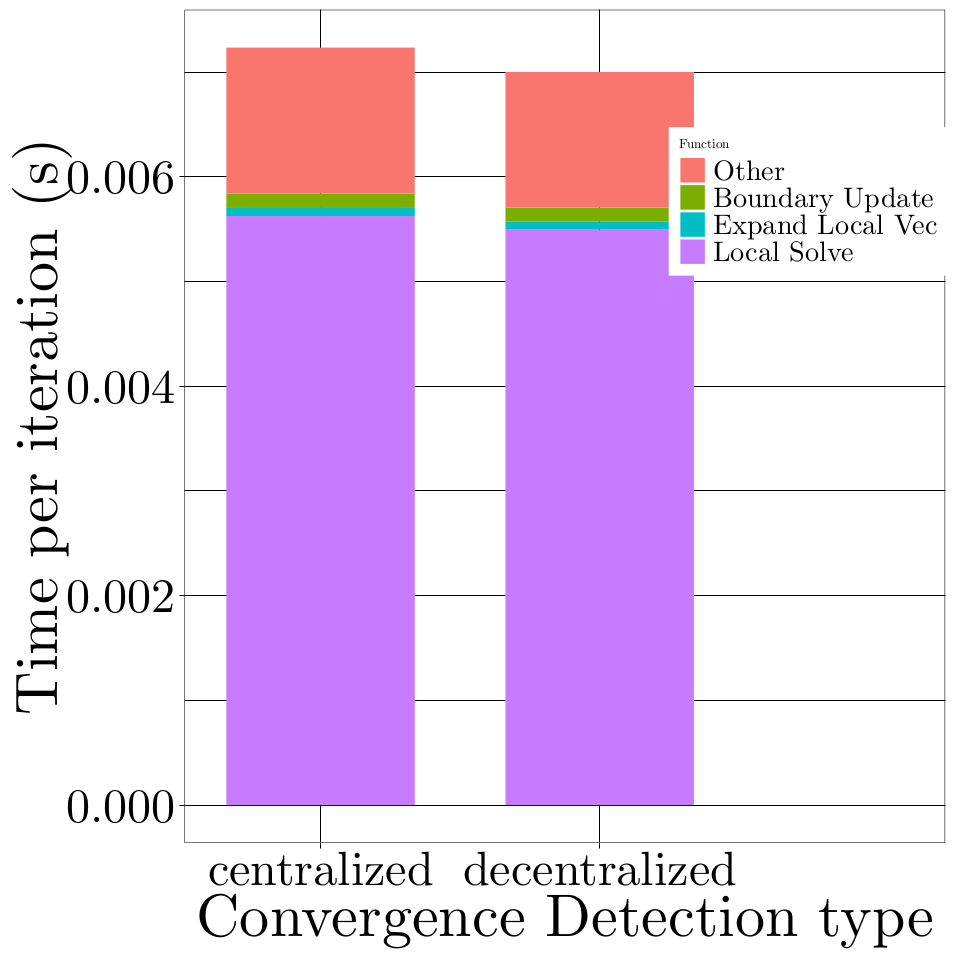
(a) Runtime Breakdown for the subdomain update

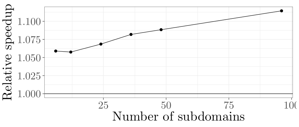
(b) Speedup - Decentralized vs Centralized

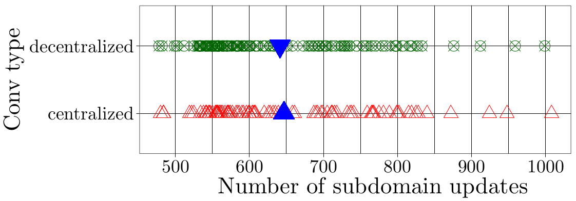
(c) Subdomain update spread

Figure 7: Comparing the centralized and decentralized convergence detection algorithms. (a) shows the time spent in different functions, (b) shows the speedup of using a decentralized vs using a centralized algorithm and (c) shows the number of subdomain updates for the two methods for all the subdomains.

4.5 Comparing convergence detection algorithms

In Figure 7(a), we compare the centralized and decentralized convergence detection strategies supported by the developed framework with all other parameters constant (asynchronous, i.e. one-sided version, metis partitioner, overlap of 16 elements, problem size 262144). As the number of subdomains increases, a centralized tree detection has a higher overhead because everything is centralized through the root, see Figure 7(b). A better understanding of the two convergence detection algorithms can be obtained from Figure 7(c) which shows the variance in the number of subdomain updates (local solves) with the average number of local solves counts indicated with blue triangles (for 96 subdomains). The decentralized algorithm is able to detect convergence slightly faster, which also reduces the time-to-solution compared to the centralized counterpart.

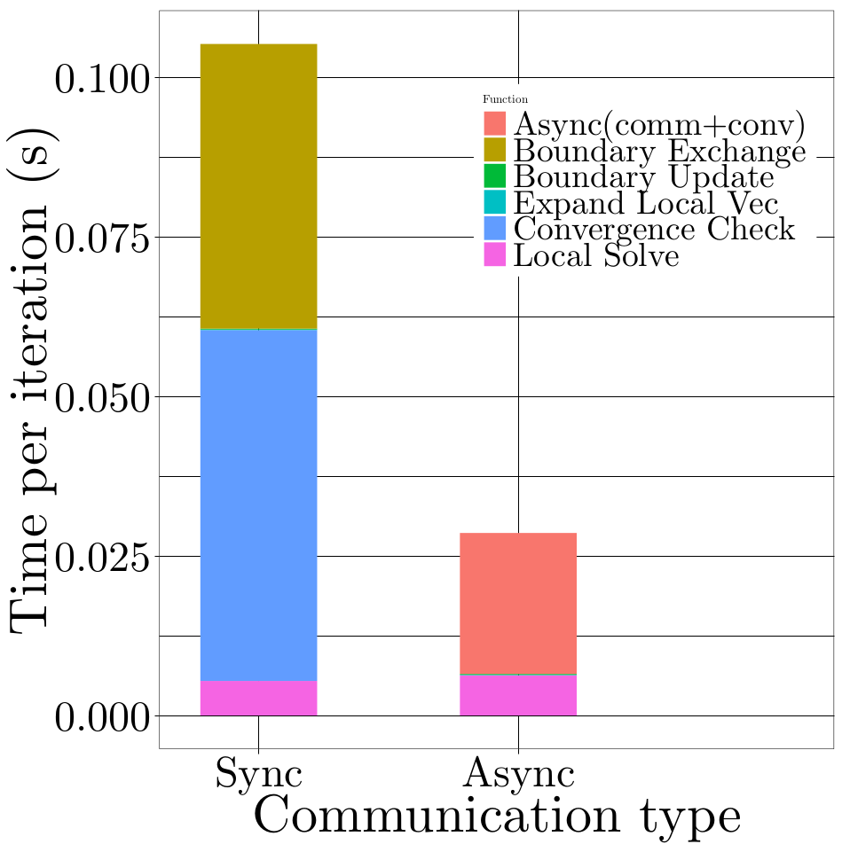
(a) Runtime breakdown for the averaged subdomain update

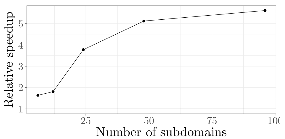
(b) Speedup - Asynchronous vs Synchronous

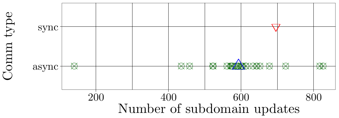
(c) Subdomain update spread

Figure 8: Comparing scaling on increasing number of comms. (a) shows the time spent in different functions, (b) shows the speedup of the asynchronous version (one-sided MPI) over the synchronous version (two-sided MPI) and (c) shows the subdomain update spread for the two versions.

4.6 Comparing two-sided and one-sided communications

We finally compare the asynchronous RAS solver (one-sided MPI) against the synchronous RAS solver (two-sided MPI) using the respectively optimal settings. Figure 8(a) compares the runtime breakdown of one subdomain update of the synchronous RAS solver with the runtime breakdown of the asynchronous RAS solver (problem size 1M, 36 subdomains, 16 overlap). Figure 8(b) relates the time-to-solution speedup of the asynchronous version over the synchronous version to the subdomain count (every subdomain handles a problem of size 4096). The speedup increases with the subdomain count, reaching a speedup of about 5.5$\times$ for 96 subdomains. In Figure 8(c), we visualize for the 36 subdomain case the number of local solves the distinct subdomains complete over the RAS solver execution. For the synchronized RAS solver, all subdomains complete the same number of local solves (even though this may not be needed as subdomains may already have converged). In the asynchronous RAS, some subdomains complete a much higher number of local solves, but the median of subdomain updates is smaller than for the synchronized RAS solver. Even with a well-balanced problem and machine setting, we see a difference of up to two in terms of the subdomain update counts between the one-sided and two-sided communication paradigms.

5 Conclusion and Future work

In this paper, we present a framework that allows to implement and compare asynchronous and synchronous iterative methods for multi-node systems featuring GPUs. The framework supports different communication schemes based on two-sided MPI (synchronous) and one-sided MPI (asynchronous). In addition, both direct and iterative local solvers are supported for a wide variety of modern HPC hardware, including CPUs, NVIDIA and AMD GPUs. We implement both centralized and decentralized convergence detection algorithms.

To study the benefits of using asynchronous iterative methods for sparse problems, we realize an asynchronous version of the Restricted Additive Schwarz algorithm and compare with the synchronous counterpart. The study is conducted on the Summit HPC system with up to 16 nodes each equipped with 6 V100 NVIDIA GPUs. We analyze the effect of different parameters such as partitioning, overlap size, and convergence detection strategy for the synchronous and asynchronous RAS solver. We also reveal that asynchronous RAS can for optimal parameter choices complete up to 5.5$\times$ faster than its synchronous counterpart.

As future work, we plan to implement and study more methods such as the Optimized Restricted Additive Schwarz ([17]) that overcomes the slow convergence of the RAS algorithm by communicating also the boundary element derivatives. We also plan to investigate the use of iterative local solves.

References

- [1] Saman Amarasinghe, Mary Hall, Richard Lethin, Keshav Pingali, Dan Quinlan, Vivek Sarkar, John Shalf, Robert Lucas, Katherine Yelick, Pavan Balanji, et al. Exascale programming challenges. In Proceedings of the Workshop on Exascale Programming Challenges, Marina del Rey, CA, USA. US Department of Energy, Office of Science, Office of Advanced Scientific Computing Research (ASCR), 2011.
- [2] Gérard M. Baudet. Asynchronous Iterative Methods for Multiprocessors. Journal of the ACM (JACM), 1978.
- [3] Andreas Frommer and Daniel B. Szyld. On asynchronous iterations. Journal of Computational and Applied Mathematics, 2000.
- [4] Daniel B. Szyld. Different models of parallel asynchronous iterations with overlapping blocks. Computational and Applied Mathematics, 17:101–115, 1998.
- [5] H A Schwarz. Ii. ueber einen grenzübergang durch alternirendes verfahren. Wolf J. XV. 272-286. 1870 (1870)., 1870.
- [6] M Dryja and O B Widlund. An Additive Variant of the {S}chwarz Alternating Method for the Case of Many Subregions. Technical Report 339, 1987.
- [7] Michele Benzi, Andreas Frommer, Reinhard Nabben, and Daniel B. Szyld. Algebraic theory of multiplicative Schwarz methods. Numerische Mathematik, 89:605–639, 2001.
- [8] Carlos Echeverría, Jörg Liesen, Daniel B. Szyld, and Petr Tichý. Convergence of the multiplicative Schwarz method for singularly perturbed convection-diffusion problems discretized on a Shishkin mesh. Electronic Transactions on Numerical Analysis, 48:40–62, 2018.
- [9] L Dolean, Victorita, Gander, Martin, Gerardo-Giorda. Optimized Schwarz methods for maxwell’s equations. SIAM Journal on Scientific Computing, 20(6):2994–3013, 2010.
- [10] Eric Blayo, David Cherel, and Antoine Rousseau. Towards Optimized Schwarz Methods for the Navier–Stokes Equations. Journal of Scientific Computing, 66(1):275–295, 2016.
- [11] Zhiyong Liu and Yinnian He. Restricted additive schwarz preconditioner for elliptic equations with jump coefficients. Advances in Applied Mathematics and Mechanics, 8(6):1072–1083, 2016.
- [12] Marcella Bonazzoli, Victorita Dolean, Ivan Graham, Euan Spence, and Pierre-Henri Tournier. Two-level preconditioners for the Helmholtz equation. pages 1–8, 2017.
- [13] Ichitaro Yamazaki, Edmond Chow, Aurelien Bouteiller, and Jack Dongarra. Performance of asynchronous optimized Schwarz with one-sided communication. Parallel Computing, 86:66–81, 2019.
- [14] Andreas Frommer and Daniel B. Szyld. On Asynchronous Iterations. Journal of Computational and Applied Mathematics, 123:201–216, 2000.
- [15] Andreas Frommer and Daniel B. Szyld. Weighted max norms, splittings, and overlapping additive Schwarz iterations. Numerische Mathematik, 83:259–278, 1999.
- [16] Xiao Chuan Cai and Marcus Sarkis. Restricted additive Schwarz preconditioner for general sparse linear systems. SIAM Journal of Scientific Computing, 1999.
- [17] Frédéric Magoulès, Daniel B. Szyld, and Cédric Venet. Asynchronous optimized Schwarz methods with and without overlap. Numerische Mathematik, 137:199–227, 2017.
- [18] Frédéric Magoulès and Cédric Venet. Asynchronous iterative sub-structuring methods. Mathematics and Computers in Simulation, 145:34–49, 2018.
- [19] José C. Garay, Frédéric Magoulès, and Daniel B. Szyld. Optimized Schwarz method for Poisson’s equation in rectangular domains. In Peter E. Bjøstard, Susanne C. Brenner, Lawrence Halpern, Hyea Hyun Kim, Ralf Kornhuber, Talal Rahman, and Olof B. Widlund, editors, Domain Decomposition Methods in Science and Engineering XXIV, volume 125 of Lecture Notes in Computer Science and Engineering, pages 533–541, Berlin and Heidelberg, 2018. Springer.
- [20] Andreas Frommer and Daniel B. Szyld. An algebraic convergence theory for restricted additive Schwarz methods using weighted max norms. SIAM Journal on Numerical Analysis, 39:463–479, 2001.
- [21] José C. Garay, Frédéric Magoulès, and Daniel B. Szyld. Convergence of asynchronous optimized Schwarz methods in the plane. In Peter E. Bjøstard, Susanne C. Brenner, Lawrence Halpern, Hyea Hyun Kim, Ralf Kornhuber, Talal Rahman, and Olof B. Widlund, editors, Domain Decomposition Methods in Science and Engineering XXIV, volume 125 of Lecture Notes in Computer Science and Engineering, pages 333–341, Berlin and Heidelberg, 2018. Springer.
- [22] Nissim Francez. Distributed Termination. ACM Transactions on Programming Languages and Systems (TOPLAS), 1980.
- [23] Friedemann Mattern. Algorithms for distributed termination detection. Distributed Computing, 1987.
- [24] Edsger W. Dijkstra, W. H.J. Feijen, and A. J.M. van Gasteren. Derivation of a termination detection algorithm for distributed computations. Information Processing Letters, 1983.
- [25] Jacques M. Bahi, Sylvain Contassot-Vivier, Raphaël Couturier, and Flavien Vernier. A decentralized convergence detection algorithm for asynchronous parallel iterative algorithms. IEEE Transactions on Parallel and Distributed Systems, 2005.
- [26] George Karypis and Vipin Kumar. METIS* A Software Package for Partitioning Unstructured Graphs , Partitioning Meshes , and Computing Fill-Reducing Orderings of Sparse Matrices. Manual, 1998.
- [27] Giovanni Alzetta, Daniel Arndt, Wolfgang Bangerth, Vishal Boddu, Benjamin Brands, Denis Davydov, Rene Gassmöller, Timo Heister, Luca Heltai, Katharina Kormann, Martin Kronbichler, Matthias Maier, Jean Paul Pelteret, Bruno Turcksin, and David Wells. The deal.II library, Version 9.0. Journal of Numerical Mathematics, 2018.
- [28] Ginkgo, a high performance numerical linear algebra library. https://github.com/ginkgo-project/ginkgo, 2020. Accessed in Jan 2020.
- [29] Hartwig Anzt, Terry Cojean, Chen Yen-Chen, Jack Dongarra, Goran Flegar, Pratik Nayak, Stanimire Tomov, Yuhsiang M. Tsai, and Weichung Wang. Load-balancing sparse matrix vector product kernels on gpus. ACM Trans. Parallel Comput., 7(1), March 2020.
- [30] Yanqing Chen, Timothy A. Davis, William W. Hager, and Sivasankaran Rajamanickam. Algorithm 887: Cholmod, supernodal sparse cholesky factorization and update/downdate. ACM Trans. Math. Softw., 35(3), October 2008.
- [31] Ruipeng Li. On parallel solution of sparse triangular linear systems in CUDA. CoRR, abs/1710.04985, 2017.
- [32] Denis Foley and John Danskin. Ultra-Performance Pascal GPU and NVLink Interconnect. IEEE Micro, 2017.
- [33] MessagePassingInterfaceForum. MPI-2 : Extensions to the Message-Passing Interface. In University of Tennessee, available online at http://www. mpi-forum. org/docs/docs. html, 2003.
- [34] James A. Kahle, Jaime Moreno, and Dan Dreps. 2.1 Summit and Sierra: Designing AI/HPC Supercomputers. In Digest of Technical Papers - IEEE International Solid-State Circuits Conference, 2019.