Cell cycle heritability and localization phase transition in growing populations

Abstract

The cell cycle duration is a variable cellular phenotype that underlies long-term population growth and age structures. By analyzing the stationary solutions of a branching process with heritable cell division times, we demonstrate existence of a phase transition, which can be continuous or first-order, by which a non-zero fraction of the population becomes localized at a minimal division time. Just below the transition, we demonstrate coexistence of localized and delocalized age-structure phases, and power law decay of correlation functions. Above it, we observe self-synchronization of cell cycles, collective divisions, and slow ‘aging’ of population growth rates.

The duration of a cell-cycle, or inter-division time (IDT), is a fluctuating quantity in cellular populations, and its statistical properties are thought to result from biological mechanisms that regulate cell growth and division Taheri-Araghi et al. (2015); Susman et al. (2018); Hashimoto et al. (2016). For single cells that grow in size exponentially, as in bacteria Taheri-Araghi et al. (2015) and yeast Nakaoka and Wakamoto (2017), models of cell-size regulation typically predict negative mother-daughter correlation of IDTs Amir (2014). Yet in a subset of bacterial experiments and in most observations on mammalian cells, positive IDT correlations have been measured (see Table S1 in ), indicating that the cell cycle duration is a heritable, fluctuating single-cell phenotype. Such heritability enables selection to act on the distribution of IDTs in a population to increase the long-term population growth rate. Here we take up the question of how selection and cell cycle heritability interact to determine long-term population dynamics, a fundamental step toward understanding how evolution has shaped cell cycle control mechanisms.

To investigate the effect of IDT heritability on population growth, we considered a model with heritable IDTs that was first introduced in Lebowitz and Rubinow (1974), which we refer to as the Lebowitz-Rubinow model below. We noticed the existence of a heritability threshold above which the population’s distribution of IDTs would localize at the minimal IDT corresponding to the fastest possible single-cell growth rate. We identify and characterize a localization phase transition in this model. We show the ancestral mean IDT provides an order parameter of the transition, and above the heritability threshold predict the emergence of arbitrarily long single cell lineages that maintain perfect inheritance of a minimal IDT. This prediction is confirmed in numerical simulations of finite populations. We observe slow punctuated dynamics above the heritability threshold, characteristic of systems that exhibit aging, as well as cell-cycle synchronization in finite populations. Our work provides fundamental connections between dynamics of age-structured populations Charlesworth (1994) and well-studied error-threshold phenomena of evolutionary theory Eigen et al. (1989); Hermisson et al. (2002), both of which are described by the unifying framework of statistical physics of phase transitions.

Model and stationary solutions.

We model a proliferating population by a branching process in which $K\left(\tau,\tau^{\prime}\right)$ is the transition probability density from $\tau^{\prime}$ to $\tau$, where $\tau^{\prime}$ and $\tau$ are the parent and offspring IDTs, respectively. To study the effect of heritability of IDTs, we focus on the analytically tractable Lebowitz-Rubinow model Lebowitz and Rubinow (1974), which uses the transition kernel

$$K\left(\tau,\tau^{\prime}\right)=\beta\delta\left(\tau-\tau^{\prime}\right)+\left(1-\beta\right)k\left(\tau\right)\ ,$$ (1)

where $\delta\left(\cdot\right)$ is the Dirac delta function, $\beta$ represents the heritability of IDTs in the model ($0\leq\beta<1$), and $k\left(\tau\right)$ is a probability density function on the interval $\left[\tau_{0},\infty\right)$, with $0<\tau_{0}<\infty$. A cell produces $\hat{z}$ offsprings at every division, where $\hat{z}$ is independently drawn from a fixed probability distribution and its average is denoted by $z>0$. For example, $z=2$ for binary division organisms and $z=1$ for the isolated single cells.

The dynamics of cell divisions in the population are governed by

$$n_{\textrm{div}}(\tau;t+\tau)=z\int_{0}^{\infty}K\left(\tau,\tau^{\prime}\right)n_{\textrm{div}}\left(\tau^{\prime};t\right)d\tau^{\prime}.$$ (2)

where $n_{\textrm{div}}\left(\tau;t\right)d\tau dt$ is the expected number of dividing cells (cells at the termination of cell-cycle) between times $t$ and $t+dt$ with IDT between $\tau$ and $\tau+d\tau$ . The expected number of divisions occurring between $t$ and $t+dt$ is given by $N_{\textrm{div}}\left(t\right)dt:=dt\int_{0}^{\infty}n_{\textrm{div}}\left(\tau;t\right)d\tau$. The time-dependent population growth rate is defined by $\Lambda_{t}:=\nicefrac{{\left(z-1\right)N_{\text{div}}\left(t\right)}}{{N\left(t\right)}}$, where $N\left(t\right)$ is the expected population size at time $t$ (see Note (1) for detailed derivations).

The steady-state, exponentially growing solution of (2) can be found by substituting the form $n_{\textrm{div}}\left(\tau;t\right)=N_{\textrm{div}}\left(t\right)\cdot p_{\textrm{div}}\left(\tau\right)$, where $p_{\textrm{div}}\left(\tau\right)$ is the stationary probability density of IDTs of dividing cells, yielding

$$p_{\mathrm{div}}\left(\tau\right)=ze^{-\Lambda\tau}\int_{0}^{\infty}K\left(\tau,\tau^{\prime}\right)p_{\mathrm{div}}\left(\tau^{\prime}\right)d\tau^{\prime}\ ,$$ (3)

Using (1) above, and solving the equation one obtains

$$p_{\textrm{div}}\left(\tau\right)=q_{\beta,z,\Lambda}\left(\tau\right):=\frac{\left(1-\beta\right)k\left(\tau\right)ze^{-\Lambda\tau}}{1-\beta ze^{-\Lambda\tau}}$$ (4)

where the steady-state growth rate $\Lambda$ is determined by the normalization condition

$$Q\left(\beta,z,\Lambda\right):=\int_{0}^{\infty}q_{\beta,z,\Lambda}\left(\tau\right)d\tau=1.$$ (5)

If $z=1$, for example, then $\Lambda=0$ and $p_{\textrm{div}}\left(\tau\right)=k\left(\tau\right)$ for any $0\leq\beta<1$. Namely, the stationary IDT distribution of isolated single cells is invariant of $\beta$. We remark that $\beta$ is the correlation coefficient of IDTs between parent and offspring for isolated, single cell growth at steady-state Note (1).

In the absence of IDT correlations ($\beta=0$), one recovers the well-known result $p_{\textrm{div}}\left(\tau\right)=ze^{-\Lambda\tau}k\left(\tau\right)$ where $\Lambda$ is the unique real root of the integral equation $z\int_{0}^{\infty}e^{-\Lambda\tau}k\left(\tau\right)d\tau=1$ Fisher (1930); Hashimoto et al. (2016). For $\beta>0$, one additionally must have $1-\beta ze^{-\Lambda\tau}>0$ for all $\tau$ in the support of $k(\tau)$ to ensure $q_{\beta,z,\Lambda}\left(\tau\right)\geq 0$. If $k(\tau)>0$ for all $\tau>\tau_{0}$, we find

$$\Lambda\geq\omega_{0}\left(\beta,z\right):=\sup_{\tau>\tau_{0}}\frac{\ln\left(\beta z\right)}{\tau}=\max\left(0,\frac{\ln\left(\beta z\right)}{\tau_{0}}\right);$$ (6)

(see Note (1) for $k(\tau)$ with bounded support). Since $Q\left(\beta,z,\Lambda\right)$ is a monotonically decreasing function of $\Lambda$ tending to zero as $\Lambda\rightarrow\infty$, Eq. 5 has a unique root $\Lambda_{\beta,z}$ provided that $Q\left(\beta,z,\omega_{0}\left(\beta,z\right)\right)\geq 1$. This condition holds for $\beta<\beta_{c}$, where $\beta_{c}$ is a critical heritability threshold defined by

$$Q\left(\beta_{c},z,\omega_{0}\left(\beta_{c},z\right)\right)=1\ ,$$ (7)

such that for $\beta>\beta_{c}$, $Q\left(\beta,z,\omega_{0}\left(\beta,z\right)\right)<1$ and Eq. 5 does not admit a real solution $\Lambda_{\beta,z}$. For $\beta>\beta_{c}$, the solution $p_{\textrm{div}}\left(\tau\right)$ given in (4) is incomplete, as there is missing probability $1-Q$. For $z>1$, the full solution is

$$p_{\textrm{div}}\left(\tau\right)=q_{\beta,z,\Lambda_{\beta,z}}\left(\tau\right)+\left(1-Q\left(\beta,z,\Lambda_{\beta,z}\right)\right)\delta\left(\tau-\tau_{0}\right)\ ,$$ (8)

and substitution into (3) yields $\Lambda_{\beta,z}=\tau_{0}^{-1}\ln\left(\beta z\right)$ for the steady-state growth rate when $\beta>\beta_{c}$ Note (1).

Further analysis of (7) shows that a heritability threshold $\beta_{c}<1$ exists if and only if $\int_{0}^{\infty}d\tau k(\tau)/(\tau-\tau_{0})$ converges; e.g. if $k(\tau)\sim(\tau-\tau_{0})^{\gamma}$ near $\tau_{0}$ for some $\gamma>0$. The steady state population growth rate $\Lambda_{\beta,z}$ qualitatively changes as $\beta$ crosses the threshold: it depends on $k\left(\tau\right)$ for $\beta<\beta_{c}$, and becomes independent of it for $\beta>\beta_{c}$. The expected number of offspring having the same IDT as their parent is $\beta z$, and only parents with $\tau^{\prime}=\tau_{0}$ can generate offspring with $\tau=\tau_{0}$. Thus, the fraction of the population with IDT $\tau_{0}$ grows with rate $\tau_{0}^{-1}\ln\left(\beta z\right)$. If we add a small fraction of $\tau_{0}$ cells to a population, they go extinct if $\beta z<1$, while if $\beta z>1$, they can constitute a giant cluster in the population’s genealogy. The subpopulation localized at $\tau=\tau_{0}$ will be outcompeted by the rest of the population for $z^{-1}<\beta<\beta_{c}$, with $\Lambda_{\beta,z}$ determined by (5); or it will dominate the population for $\beta>\beta_{c}$, and thus dictate its growth rate to be $\Lambda_{\beta,z}=\tau_{0}^{-1}\ln\left(\beta z\right)$. In Fig. 1A, we show a range of examples $k(\tau)$ which admit a threshold $\beta_{c}$. Increasing $\beta$ from 0 to 1, $\Lambda_{\beta,z}$ increases monotonically with a shallow slope, while past $\beta_{c}$, the slope of the growth rate changes markedly (Fig. 1B).

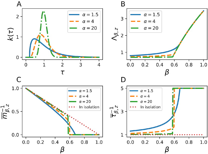
Figure 1: Stationary solutions and their dependence on the heritability parameter $\beta$. (A) The IDT distribution, $k\left(\tau\right)$, is chosen to be a gamma distribution, shifted by $\tau_{0}=0.2$, with shape parameters $\alpha=1.5$, $4$, and $20$; $k\left(\tau\right)=\Gamma\left(\alpha\right)^{-1}\theta^{-\alpha}\left(\tau-\tau_{0}\right)^{\alpha-1}e^{-\nicefrac{{\left(\tau-\tau_{0}\right)}}{{\theta}}}$ for $\tau\geq\tau_{0}$. For the mean IDT to be 1, the scale parameter $\theta$ is chosen as $\tau_{0}+\alpha\theta=1$. (B-D) Dependence of key quantities of the stationary solutions on $\beta$ using $z=2$; all other parameters are the same as in A. $\beta_{c}=0.68$, $0.60$ and $0.58$ respectively for $\alpha=1.5$, $4$, and $20$. (B) Population growth rate, $\Lambda_{\beta,z}$. (C) Reciprocal mean block size, $\overline{m}_{\beta,z}^{-1}$. (D) Reciprocal ancestral mean IDT, $\overline{\tau}_{\beta,z}^{-1}$.

Localization phase transition of population age structure.

We now show that the threshold behavior identified above constitutes a phase transition in the strict sense. We map the population to a statistical mechanical ensemble, as follows. From the viewpoint of single cell lineages – i.e. the history of an individual and all of its ancestors – an age-structured population constitutes an ensemble of trajectories: the sequence of IDTs along a lineage $(\dots,\tau_{i-1},\tau_{i},\tau_{i+1},\ldots)$ is analogous to a microscopic state of a large system (e.g. configuration of spins on a lattice, conformation of a polymer in space, etc.); while a single ancestral cell division $\tau_{i}$ specifies the state of a single component (e.g a spin, or a monomer). The population is an ensemble of lineages, and the steady-state population growth rate is its free energy Note (1); Wakamoto et al. (2012).

To analyze the structure of lineages observed above and below $\beta_{c}$, we consider the number of generations with which the same IDT is consecutively inherited, which we denote by $m$ and call the “block size”. The probability distribution of $m$ over lineages is analogous to a correlation function, and its mean measures the typical correlation length. To compute these quantities, we let $\left(\tau^{\prime},\tau\right)$ denote a pair of IDTs, where $\tau^{\prime}$ and $\tau$ are parent and offspring IDTs, respectively. From (3) one can infer that the stationary probability density to find $\left(\tau^{\prime},\tau\right)$ is $ze^{-\Lambda\tau}K\left(\tau,\tau^{\prime}\right)p_{\textrm{div}}\left(\tau^{\prime}\right)$. In particular, the probability of observing $(\tau,\tau)$ is $\beta ze^{-\Lambda\tau}p_{\textrm{div}}\left(\tau\right)$. Repeatedly multiplying $\beta ze^{-\Lambda_{\beta,z}\tau}$, the probability for $\tau$ drawn from $p_{\textrm{div}}\left(\tau\right)$ to be inherited at least $m-1$ times is $\left(\beta ze^{-\Lambda_{\beta,z}\tau}\right)^{m-1}$, hence the joint probability distribution of block size $m$ and IDT $\tau$ is

$$p_{\textrm{lin}}\left(m,\tau\right):=\left(1-\beta ze^{-\Lambda_{\beta,z}\tau}\right)\left(\beta ze^{-\Lambda_{\beta,z}\tau}\right)^{m-1}p_{\textrm{div}}\left(\tau\right)\ .$$ (9)

For $\beta<\beta_{c}$, the mean block size on lineage is

$$\overline{m}_{\beta,z}:=\sum_{m\geq 1}\int_{0}^{\infty}m\cdot p_{\textrm{lin}}\left(m,\tau\right)d\tau<\infty\ ,$$ (10)

and the probability distribution of IDT on lineage, also known as the ancestral distribution Hermisson et al. (2002), is

$$p_{\textrm{lin}}\left(\tau\right):=\frac{\sum_{m\geq 1}m\cdot p_{\textrm{lin}}\left(m,\tau\right)}{\overline{m}_{\beta,z}}\ ,$$ (11)

and represents the probability distribution of IDTs of ancestors in the infinite past Note (1). For $\beta>\beta_{c}$, $\overline{m}_{\beta,z}$ diverges and $p_{\textrm{lin}}\left(\tau\right)$ must be computed as an appropriate limit Note (1); we obtain

$$p_{\textrm{lin}}\left(\tau\right)=\begin{cases}\begin{array}[]{c}\frac{\left(1-\beta\right)k\left(\tau\right)ze^{-\Lambda_{\beta,z}\tau}}{\overline{m}_{\beta,z}\left(1-\beta ze^{-\tau\Lambda_{\beta,z}}\right)^{2}},\\ \delta\left(\tau-\tau_{0}\right),\end{array}&\begin{array}[]{c}0\leq\beta<\beta_{c}\\ \beta_{c}<\beta<1\end{array}\end{cases}\ .$$ (12)

The expression indicates that the IDT distribution on lineages in the population is localized entirely at $\tau=\tau_{0}$ above $\beta_{c}$, despite the fact that the IDT distribution of isolated lineages remains $k\left(\tau\right)$.

The mean block size $\overline{m}_{\beta,z}$ serves as an order parameter that diverges for $\beta>\beta_{c}$, and the continuity of the phase transition can be characterized by its behavior near $\beta_{c}$. If $\lim_{\beta\uparrow\beta_{c}}\overline{m}_{\beta,z}=\infty$, the transition is a continuous phase transition, while if $\lim_{\beta\uparrow\beta_{c}}\overline{m}_{\beta,z}<\infty$ the transition is referred to as discontinuous, or ‘first-order’. Analogously, the lineage mean IDT, $\overline{\tau}_{\beta,z}:=\int_{0}^{\infty}\tau p_{\text{lin}}\left(\tau\right)d\tau$, which is given by $\partial\Lambda_{\beta,z}/\partial\log z$ (i.e. a first-order derivative of the free energy Note (1)), exhibits the same type of phase transition. Examples of the $\beta$ dependence of $\overline{m}_{\beta,z}$ and $\overline{\tau}_{\beta,z}$ are shown in Fig. 1C and D. Assuming the law of large numbers, $\overline{\tau}_{\beta,z}^{-1}\simeq\nicefrac{{D}}{{t}}$ and $\overline{m}^{-1}_{\beta,z}\simeq\nicefrac{{S}}{{D}}$ hold where $D$ and $S$ denote the number of divisions and the number of switches to different values of $\tau$ on lineage, respectively Note (1).

Using the form of $k\left(\tau\right)$ as in Fig. 1, where $k(\tau)\sim(\tau-\tau_{0})^{\gamma}$ for $\tau$ near $\tau_{0}$, and computing $\overline{m}_{\beta,z}$ we find that the phase transition is continuous for $0<\gamma\leq 1$, and becomes discontinuous for $\gamma>1$. For the latter type of transition, one expects to observe coexistence of two phases at the transition point, which is seen in numerical simulations of finite populations shown below (Fig. 2B). We can also compute the marginal probability distribution $p_{\textrm{lin}}^{\textrm{M}}\left(m\right)$ of block size $m$, which decays exponentially below the transition, and follows power law statistics, $p_{\textrm{lin}}^{\textrm{M}}\left(m\right)\sim m^{-\gamma-1}$ for large $m$, in the limit $\beta\uparrow\beta_{c}$ as expected for correlation functions in the vicinity of a phase transition Note (1). Such an appearance of long memory of IDT inheritance at the transition point is likewise observed in simulations (Fig. 2B).

Aging of long-term growth rate in finite populations.

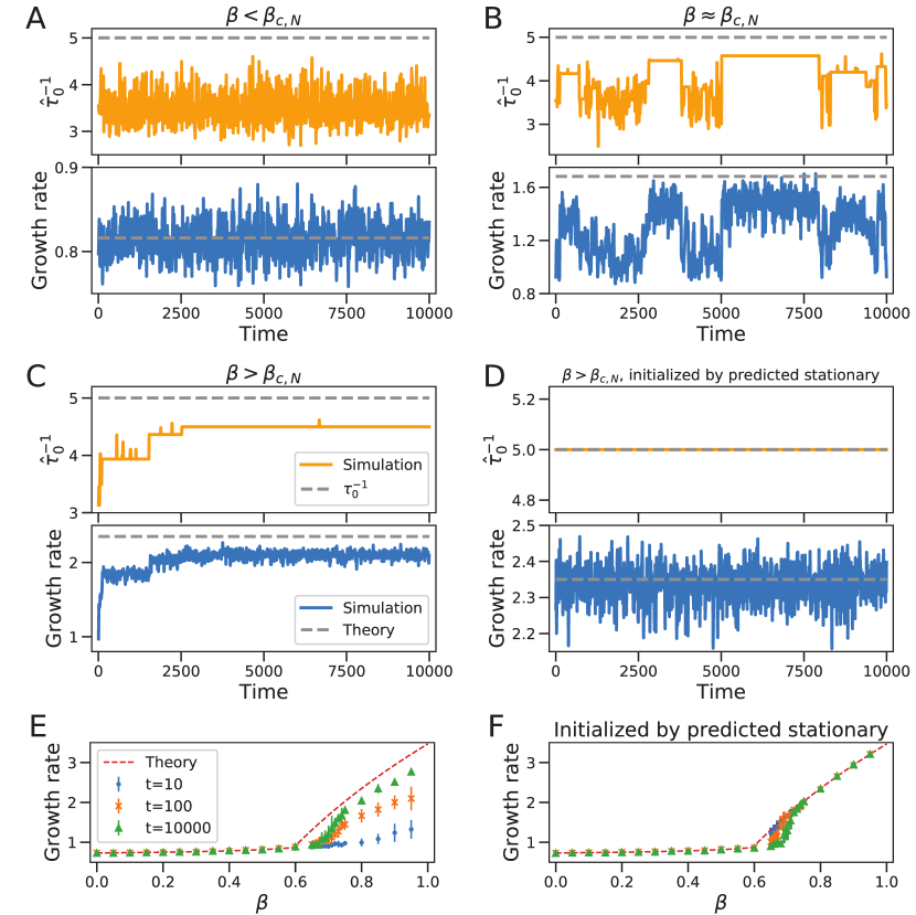
Figure 2: Aging of growth rates in a finite population. The parameters are as in Fig. 1 using $\alpha=4$, which exhibits a first-order localization transition. In simulations, some of the cells in the population may be removed when newborn cells appear in order to keep the population size $N=100$ constant. See Note (1) for simulation details. $\beta_{c,N}=0.73$. (A-D) Time courses of reciprocal empirical minimal IDT $\hat{\tau}_{0}^{-1}$ (top, orange, solid) compared with the minimal IDT $\tau_{0}^{-1}$ (gray, dashed line) and growth rates (bottom, blue, solid) compared with predicted stationary value (gray, dashed line). (A) is below the transition ($\beta=0.5$) and the initial state is sampled from the delocalized state. (B) shows coexistence of delocalized and localized states ($\beta=0.7$, starting from the delocalized state). Time courses of growth rates are compared to $\hat{\tau}_{0}^{-1}\log\left(\beta z\right)$ (orange dot). (C) Time courses above the transition showing aging dynamics ($\beta=0.8$, starting from the delocalized state). (D) For $\beta=0.8$, when the initial population is sampled from predicted stationary solution, the growth rates fluctuate around the theoretically predicted stationary growth rate. (E, F) Growth rate vs $\beta$. The initial condition was chosen as delocalized state for (E) and predicted stationary for (F). For each $\beta$ and stationary conditions, 10 simulations were run, and the mean is plotted with error bars showing the standard deviation.

In finite sized populations, the stationary distribution (8) for $\beta>\beta_{c}$ is not achievable because any parent cell with IDT $\tau^{\prime}>\tau_{0}$ has probability zero of generating offspring with IDT $\tau_{0}$. Additionally, the distribution (8) cannot be maintained as a steady-state because cells with IDT $\tau_{0}$ can be lost from the population within finite time due to coalescence. To observe dynamics in finite populations, we conducted exact stochastic simulations in which cells are randomly removed to maintain a fixed population size Note (1). We sampled the initial population with size $N=100$ independently from the stationary probability distribution with $\beta=0$, which we refer to as the delocalized state, and simulated the population forward in time for a given value of $\beta>0$.

In simulations with $\beta<\beta_{c}$, growth rates $\Lambda_{t}$ fluctuate around the expected steady-state growth rate (Fig. 2A). For $\beta$ slightly above $\beta_{c}$, however, $\Lambda_{t}$ exhibits sudden transitions between two distinct, long-lived states (Fig 2B), which is expected for systems near a first-order phase transition. One of these states represents localization at the empirical minimum IDT, denoted by $\hat{\tau}_{0}$, which is the minimum IDT among all the dividing cells within each time bin Note (1). In this state, the growth rate fluctuates around $\hat{\tau}_{0}^{-1}\ln\left(\beta z\right)$ over a sufficient period during which $\hat{\tau}_{0}$ is constant. The other phase represents delocalization, where $\hat{\tau}_{0}$ exhibits large fluctuations. For higher values of $\beta$, the observed growth rate increases stepwise and fluctuates around $\hat{\tau}_{0}^{-1}\ln\left(\beta z\right)$ (Fig. 2C). In this case, a fraction of the population localized at $\hat{\tau}_{0}$ is maintained over a significant time interval until a new value of $\hat{\tau}_{0}$ replaces the current empirical minimum IDT. The time intervals between these replacement events become increasingly long as $\hat{\tau}_{0}$ approaches $\tau_{0}$, because IDTs that are shorter than the current minimum become increasingly rare. When the simulation starts with the population sampled from the predicted stationary probability distribution with the same $\beta$ used in Fig. 2C, $\Lambda_{t}$ fluctuates around $\hat{\tau}_{0}^{-1}\ln\left(\beta z\right)$ and $\hat{\tau}_{0}=\tau_{0}$ is preserved over the entire simulation time (Fig. 2D). Values of $\Lambda_{t}$ at different simulation times are plotted as function of $\beta$ initialized at either the delocalized state (Fig. 2E) or the predicted stationary solution (Fig. 2F). For both initial conditions, the curve at $t=10^{4}$ possesses an inflection point $\beta_{c,N}$ slightly greater than $\beta_{c}$, which we refer to as the effective transition point at fixed population size $N$ (see Note (1) for detailed definition). For both of these initial conditions, the population would reach the steady-state where $\hat{\tau}_{0}$ fluctuates around some specific $\tau_{\textrm{opt}}\left(>\tau_{0}\right)$ but it was not observed in reasonable simulation time due to the observed aging behavior of the dynamics. Despite this challenge in numerically observing the true steady-state, due to the slow aging of the dynamics, our finite population simulations demonstrate the existence of the transition point above which the localized phase emerges in the dynamics, and that the dependence of the observed growth rate on $\beta$ is quantitatively predicted by theoretical analysis of the stationary solution.

Collective divisions and cell cycle synchronization.

In addition to aging dynamics, we observed collective divisions within the population above the transition (Fig. 3). The number of divisions that occurred, binned in short intervals, is plotted over time. Compared to Figs. 3A and C, Fig. 3E shows division events occurring collectively and periodically. Its auto-correlation function does not oscillate below the transition (3B), but exhibits decaying oscillations near the transition point (3D) and sustained oscillations above the transition (3F). The fact that the period of the autocorrelation function is close to $\tau_{0}$ reflects localization at $\hat{\tau}_{0}$ close to $\tau_{0}$. We also tested the robustness of the transition properties to noise in the inheritance of IDTs by allowing small fluctuations of the offspring’s IDT when it inherits its parent’s IDT with probability $\beta$. To do so, we modified the transition kernel to be

$$K\left(\tau,\tau^{\prime}\right)=\beta p_{\text{norm}}\left(\tau-\tau^{\prime},\sigma\right)+\left(1-\beta\right)k\left(\tau\right)$$ (13)

where $p_{\textrm{norm}}\left(x,\sigma\right)$ is a normal distribution density function with standard deviation $\sigma$, truncated at $\tau_{0}$. As a result, the population can reach equilibrium over a reasonable time scale, that is, the long-term behaviors coincide between the two distinct initial conditions (Figs. S6 and S7 in Note (1)). Even without exact inheritance of parental IDTs, signatures of the phase transition are still observed (Figs. S8-S15 in Note (1)). Collective divisions are weaker but still detectable through the decaying oscillations of the autocorrelation function of divisions in population (Figs. S16 and S17 in Note (1)). Division rate oscillations have also been predicted to arise in cell size control models, due to negative IDT correlations Jafarpour (2019).

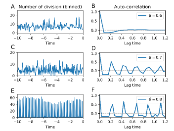
Figure 3: Synchronization of cell-cycles above the transition. The simulation is initialized by the delocalized state. The parameters are as in Fig. 2 using $\alpha=4$ and $N=100$. $\beta_{c,N}=0.73$. Number of divisions binned over 0.1 doubling time (A, C, E) and their auto-correlations (B, D, F) are shown. Simulations are run over $10^{4}$ time units and the last 10 time units of the series are shown for A, C and E, where time point 0 indicates the simulation end. Auto-correlations are computed over entire time series. The correlation coefficient is normalized to equal 1 at zero lag. Dotted line indicates zero correlation. (A,B) Below the transition ($\beta=0.6$) timing of divisions are not synchronized. (C, D) Near the transition point ($\beta=0.7$), timing of divisions are partially synchronized, observed as decaying oscillation of the auto-correlation function. (E, F) Above the transition ($\beta>\beta_{c,N}$), collective divisions are observed indicating self-synchronization of cell cycles.

Discussion.

We analyzed how the strength of the inter-division time heritability affects age-structured population dynamics. In a model with heritable cell cycle durations first introduced in Lebowitz and Rubinow (1974), we demonstrated the existence of a localization phase transition. While the existence of a heritability threshold $\beta_{c}$ was not explicitly suggested in Lebowitz and Rubinow (1974), the potential limit on the validity of the stationary solution was pointed out. A similar localization transition in exponentially growing populations is known in mutation-selection models of theoretical population genetics Eigen (1971); Kingman (1978); Hermisson et al. (2002). For example, Kingman’s house-of-cards model Kingman (1978) describes population dynamics on a specific type of fitness landscape, which exhibits localization at maximal fitness below a critical mutation rate. The localization phase transition as a stationary state in the house-of-cards model can be generalized to include cases where fitness is correlated between parent and offspring, and the existence and the uniqueness of the stationary solutions has been proven using the theory of positive linear operators Bürger and Bomze (1996).

We showed that the signature of localization phase transition can be observed even in finite populations as small as 100 cells, which is comparable to the capacity allowed by typical microfluidic experiments Wallden and Elf (2011); Lambert and Kussell (2014); Hashimoto et al. (2016), indicating that this transition could in principle be experimentally observed. Above the transition, population growth rates exhibit aging dynamics. Similar phenomena are seen in evolution in random unbounded fitness landscape with rare mutation rate in finite population, known as the “diluted record process” Park and Krug (2008) or “successional mutation regime” Brotto et al. (2016). While the distribution and auto-correlation of individual fitness are difficult to measure in reality, measuring those of IDTs is highly feasible using in vivo single cell tracking in microfluidics-based experiments. The aging dynamics we observed in age-structured populations are closely related to the emergence of self-synchronized cell-cycles (Fig. 3). Future work on the spectral structure of the linear semigroup of age-structured population dynamics Webb (1986); Boulanouar (2011) may further elucidate the emergence of synchronized growth above the transition.

While aging dynamics above the transition are specific to the noiseless inheritance of IDT, we found that the signature of localization and self-synchronization can still be observable in “noisier” inheritance systems. This result indicates that our analytical results are applicable to real biological systems in which IDT heritability is noisy. The Lebowitz-Rubinow model does not include cell-cell interactions which are thought to be a major mechanism for cell-cycle synchronization. Remarkably, our analysis predicts strong but imperfect correlation may be enough to cause self-synchronization of cell cycles in finite populations in the absence of cell-cell interactions. Our findings could provide a basis for the design of new types of synthetic biological oscillators which leverage population-level selective forces to establish robust cell cycle synchronization and to support sustained oscillations.

We thank Yuichi Wakamoto for discussions. This work was supported by NIH grant R01-120231 to E.K.

References

- Taheri-Araghi et al. (2015) S. Taheri-Araghi, S. Bradde, J. T. Sauls, N. S. Hill, P. A. Levin, J. Paulsson, M. Vergassola, and S. Jun, Curr. Biol. 25, 385 (2015).
- Susman et al. (2018) L. Susman, M. Kohram, H. Vashistha, J. T. Nechleba, H. Salman, and N. Brenner, Proc. Natl. Acad. Sci. U. S. A. 115, 201615526 (2018), arXiv:1805.05058 .
- Hashimoto et al. (2016) M. Hashimoto, T. Nozoe, H. Nakaoka, R. Okura, S. Akiyoshi, K. Kaneko, E. Kussell, and Y. Wakamoto, Proc. Natl. Acad. Sci. 113, 3251 (2016).
- Nakaoka and Wakamoto (2017) H. Nakaoka and Y. Wakamoto, PLoS Biol. 15, e2001109 (2017).
- Amir (2014) A. Amir, Phys. Rev. Lett. 112, 208102 (2014).
- Note (1) Supplemental Material at [URL will be inserted by publisher].
- Lebowitz and Rubinow (1974) J. L. Lebowitz and S. I. Rubinow, J. Math. Biol. 1, 17 (1974).
- Charlesworth (1994) B. Charlesworth, Evolution in Age-Structured Populations, 2nd ed., Cambridge Studies in Mathematical Biology (Cambridge University Press, 1994).
- Eigen et al. (1989) M. Eigen, J. McCaskill, and P. Schuster, Adv. Chem. Phys 75, 149 (1989).
- Hermisson et al. (2002) J. Hermisson, O. Redner, H. Wagner, and E. Baake, Theor. Popul. Biol. 62, 9 (2002).
- Note (2) IDTs of sibling cells may be correlated, which does not change Eq. (2), as long as the number of offspring is independent of the parent’s IDT.
- Fisher (1930) R. Fisher, The Genetical Theory of Natural Selection (Clarendon, 1930).
- Wakamoto et al. (2012) Y. Wakamoto, A. Y. Grosberg, and E. Kussell, Evolution (N. Y). 66, 115 (2012).
- Jafarpour (2019) F. Jafarpour, Phys. Rev. Lett. 122, 118101 (2019), arXiv:1809.10217 .
- Eigen (1971) M. Eigen, Naturwissenschaften 58, 465 (1971).
- Kingman (1978) J. F. C. Kingman, J. Appl. Probab. 15, 1 (1978).
- Bürger and Bomze (1996) R. Bürger and I. M. Bomze, Adv. Appl. Probab. 28, 227 (1996).
- Wallden and Elf (2011) M. Wallden and J. Elf, Curr. Opin. Biotechnol. 22, 81 (2011).
- Lambert and Kussell (2014) G. Lambert and E. Kussell, PLoS Genet. 10, e1004556 (2014).
- Park and Krug (2008) S. C. Park and J. Krug, J. Stat. Mech. Theory Exp. 2008, 10.1088/1742-5468/2008/04/P04014 (2008), arXiv:0711.1989 .
- Brotto et al. (2016) T. Brotto, G. Bunin, and J. Kurchan, J. Stat. Mech. Theory Exp. 2016, 10.1088/1742-5468/2016/03/033302 (2016), arXiv:1407.4669 .
- Webb (1986) G. F. Webb, J. Math. Biol. 23, 269 (1986).
- Boulanouar (2011) M. Boulanouar, J. Evol. Equations 11, 531 (2011).