Dynamics of Chiral Cosmology

Abstract

We perform a detailed analysis for the dynamics of Chiral cosmology in a spatially flat Friedmann-Lemaître-Robertson-Walker universe with a mixed potential term. The stationary points are categorized in four families. Previous results in the literature are recovered while new phases in the cosmological evolution are found. From our analysis we find nine different cosmological solutions, the eight describe scaling solutions, where the one is that of a pressureless fluid, while only one de Sitter solution is recovered.

I Introduction

A detailed analysis of the recent cosmological observations dataacc1 ; dataacc2 ; data1 ; data2 ; Hinshaw:2012aka ; Ade:2015xua indicates that the universe has gone through two acceleration phases during its evolution. In particular into a late-time acceleration phase which is attributed to dark energy, and into an early acceleration phase known as inflation. Inflation was proposed four decades ago guth in order to explain why in large scales the universe appears isotropic and homogeneous. The inflationary era is described by a scalar field known as the inflaton which when dominates drives the dynamics of the universe such that the observations are explained.

In addition, scalar fields have been used to describe the recent acceleration epoch of the universe, that is, they have been applied as a source of the dark energy Ratra . In scalar field theory the gravitational field equations remain of second-order with extra degrees of freedom as many as the scalar fields and corresponding conservation equations hor1 ; hor2 ; hor3 . These extra degrees of freedom can attribute the geometrodynamical degrees of freedom provided by invariants to the modification of Einstein-Hilbert action in the context of modified/alternative theories of gravity mod1 ; mod2 ; mod3 .

The simplest scalar field theory proposed in the literature is the quintessence model Ratra . Quintessence is described by a minimally coupled scalar field $\phi\left(x^{\kappa}\right)~{}$with a potential function $V\left(\phi^{\kappa}\right)$. The scalar field satisfies the weak energy condition, i.e. $\rho\geq 0,~{}\rho+p\geq 0,$ while the equation of state parameters $w_{Q}=\frac{p}{\rho}$ is bounded as $\left|w_{Q}\right|\leq 1$. For some power-law quintessence models, the gravitational field equations provide finite-time singularities during inflation leading to chaotic dynamics sing ; page . On the other hand, for some kind of potentials the quintessence can describe the late-time acceleration udm .

In the cosmological scenario of a Friedmann-Lemaître-Robertson-Walker universe (FLRW) exact and analytic solutions of the field equations for different potentials are presented in jdbnew ; muslinov ; ellis ; barrow1 ; newref2 ; ref001 ; ref002 and references therein. Results of similar analysis on the dynamics of quintessence models are summarized in the recent review gen01 . Other scalar field models which have been proposed in the literature are: phantom fields, Galileon, scalar tensor, multi-scalar field models and others ph1 ; ph2 ; ph3 ; ph4 ; ph5 ; ph7 ; ph8 ; ph9 ; ph10 ; ph11 . Multi-scalar field models have been used to provide alternative models for the description of inflation hy1 ; hy2 ; hy3 , such as hybrid inflation, double inflation, $\alpha$-attractors hy4 ; atr1 ; atr3 and as alternative dark energy models.

Multi-scalar field models which have drawn the attention of cosmologists are, the quintom model and the Chiral model. A common feature of these two theories is that they are described by two-scalar fields, namely $\phi\left(x^{\kappa}\right)$ and $\psi\left(x^{\kappa}\right)$. For the quintom model, one of the two fields is quintessence while the second scalar field is phantom which means that the energy density of the field can be negative. One of the main characteristics of quintom cosmology is that the parameter for the equation of state for the effective cosmological fluid can cross the phantom divide line more than once qq1 ; qq2 . The general dynamics of quintom cosmology is presented in qq3 .

In Chiral theory, the two scalar fields have a mixed kinetic term. The two scalar fields are defined on a two-dimensional space of constant nonvanishing curvature atr6 ; atr7 . That model is inspired by the non-linear sigma cosmological model sigm0 . Chiral cosmology is linked with the $\alpha-$attractor models atr3 . Exact solutions and for specific cases the dynamics of Chiral cosmology were studied before in andimakis , while analytic solutions in Chiral cosmology are presented in 2sfand . In the latter reference, it was found that pressureless fluid is provided by the model, consequently, the model can also be seen as an alternative model for the description of the dark sector of the universe. Last but not least scaling attractors in Chiral theory were studied in andimakis ; per1 .

In this piece of work we are interested in the evolution of the dynamics for the gravitational field equations of Chiral cosmology in a spatially flat FLRW background space. We consider a general scenario where an interaction term for the two scalar fields exists in the potential term $V\left(\phi,\psi\right)$ of the two fields, that is, $V_{,\phi\psi}\neq 0$. Specifically, we determine the stationary points of the cosmological equations and we study the stability of these points. Each stationary point describes a solution in the cosmological evolution. Such an analysis is important in order to understand the general behaviour of the model and to infer about its viability. This approach has been applied in various gravitational theories with important results for the viability of specific theories of gravity, see for instance dyn1 ; dyn2 ; dyn3 ; dyn4 ; dyn5 ; dyn6 ; dyn7 ; dyn8 ; dyn9 and references therein. From such an analysis we can conclude about for which eras of the cosmological history can be provided by the specific theory, we refer the reader in the discussion of dyn1 . The plan of the paper is as follows.

In Section II we present the model of our consideration which is that of Chiral cosmology in a spatially flat FLRW spacetime with a mixed potential term. We write the field equations which are of second-order. By using the energy density and pressure variables we observe that the interaction of the two fields depends on the pressure term. In Section III, we rewrite the field equations by using dimensionless variables in the $H-$normalization. We find an algebraic-differential dynamical system consists of one algebraic constraint and six first-order ordinary differential equations. We consider a specific form for the potential in order to reduce dynamical system the system by one-dimension; and with the use of the constraint equation we end with a four-dimensional system.

The main results of this work are presented in Section IV. We find the stationary points of the field equations which form four different families. The stationary points of family A are those of quintessence, in family B only the kinetic part of the second scalar field contributes to the cosmological solutions. On the other hand, the points of family C are those where only the dynamic part of the second field contributes. Furthermore, for the cosmological solutions at the points of family D all the components of the second field contributes to the cosmological fluid. For all the stationary points we determine the physical properties which describe the corresponding exact solutions, as also we determine the stability conditions. An application of this analysis is presented in Section V with some numerical results. Moreover, for completeness of our study we present an analytic solution of the field equations by using previous results of the literature, from where we can verify the main results of this work. In Section VII we discuss the additional stationary points when matter source is included in the cosmological model. Finally, in Section VIII we draw our conclusions.

II Chiral cosmology

We consider the gravitational Action Integral to be 2sfand

$$S=\int\sqrt{-g}dx^{4}R-\int\sqrt{-g}dx^{4}\left(\frac{1}{2}g^{\mu\nu}H_{AB}\left(\Phi^{C}\right)\nabla_{\mu}\Phi^{A}\nabla_{\nu}\Phi^{B}+V\left(\Phi^{C}\right)\right)$$ (1)

where $\Phi^{A}=\left(\phi\left(x^{\mu}\right),\psi\left(x^{\mu}\right)\right)$, $H_{AB}\left(\Phi^{C}\right)$ is a second rank tensor which defines the kinetic energy of the scalar fields, while $V\left(\Phi^{C}\right)$ is the potential.

The Action Integral (1) describes a interacting two-scalar field cosmological model where the interaction follows by the potential $V\left(\Phi^{C}\right)=V\left(\phi,\psi\right),$ and the kinetic part.

In this work we assume that $H_{AB}\left(\Phi^{C}\right)$ is diagonal and admits at least one isometry such that (1)

$$S=\int\sqrt{-g}dx^{4}R-\int\sqrt{-g}dx^{4}\left(\frac{1}{2}g^{\mu\nu}\left(\phi_{;\mu}\phi_{;\nu}+M\left(\phi\right)\psi_{;\mu}\psi_{;\mu}\right)+V\left(\Phi^{C}\right)\right)$$ (2)

where $M\left(\phi\right)_{,\phi}\neq 0$ and $M\left(\phi\right)\neq M_{0}\phi^{2}$. In the latter two cases, $H_{AB}\left(\Phi^{C}\right)$ describe a two-dimensional flat space and if it is of Lorentzian signature then it describes the quintom model. Functional of forms of $M\left(\phi\right)$ where $H_{AB}\left(\Phi^{C}\right)$ is a maximally symmetric space of constant curvature $R_{0}$, are given by the second-order differential equation

$$2M_{,\phi\phi}M-\left(M_{,\phi}\right)^{2}+2M^{2}R_{0}=0.$$ (3)

A solution of the latter equation is $M\left(\phi\right)=M_{0}e^{\kappa\phi}$, which can be seen as the general case since new fields can be defined under coordinate transformations to rewrite the form of $H_{AB}\left(\Phi^{C}\right)$. This is the case of Chiral model that we study in this work.

Variation with respect to the metric tensor of (1) provides the gravitational field equations

$$G_{\mu\nu}=H_{AB}\left(\Phi^{C}\right)\nabla_{\mu}\Phi^{A}\nabla_{\nu}\Phi^{B}-g_{\mu\nu}\left(\frac{1}{2}g^{\mu\nu}H_{AB}\left(\Phi^{C}\right)\nabla_{\mu}\Phi^{A}\nabla_{\nu}\Phi^{B}+V\left(\Phi^{C}\right)\right),$$ (4)

while variation with respect to the fields $\Phi^{A}$ give the Klein-Gordon vector-equation

$$g^{\mu\nu}\left(\nabla_{\mu}\left(H_{~{}B}^{A}\left(\Phi^{C}\right)\nabla_{\nu}\Phi^{B}\right)\right)+H_{~{}B}^{A}\left(\Phi^{C}\right)\frac{\partial V\left(\Phi^{C}\right)}{\partial\Phi^{B}}=0.$$ (5)

According to the cosmological principle, the universe in large scales is isotropic and homogeneous described by the spatially flat FLRW spacetime with line element

$$ds^{2}=-dt^{2}+a^{2}\left(t\right)\left(dx^{2}+dy^{2}+dz^{2}\right).$$ (6)

where $a\left(t\right)$ denotes the scale factor and the Hubble function is defined as $H\left(t\right)=\frac{\dot{a}}{a}$.

For the line element (6) and the second-rank tensor $H_{AB}\left(\Phi^{C}\right)$ of our consideration the field equations are written as follows

$$3H^{2}=\frac{1}{2}\left(\dot{\phi}^{2}+M\left(\phi\right)\dot{\psi}^{2}\right)+V\left(\phi\right)+M\left(\phi\right)U\left(\psi\right),$$ (7)

$$2\dot{H}+3H^{2}=-\left(\frac{1}{2}\left(\dot{\phi}^{2}+M\left(\phi\right)\dot{\psi}^{2}\right)-V\left(\phi\right)-M\left(\phi\right)U\left(\psi\right)\right),$$ (8)

$$\ddot{\phi}+3H\dot{\phi}-\frac{1}{2}M_{,\phi}\dot{\psi}^{2}+V_{,\phi}\left(\phi\right)+M_{,\phi}U\left(\psi\right)=0,$$ (9)

$$\ddot{\psi}+3H\dot{\psi}+\frac{M_{,\phi}}{M}\dot{\phi}\dot{\psi}+U_{,\psi}=0.$$ (10)

where we replaced $V\left(\phi,\psi\right)=V\left(\phi\right)+M\left(\phi\right)U\left(\psi\right)$ and we have assumed that the fields $\phi,\psi$ inherit the symmetries of the FLRW space such that $\phi\left(x^{\mu}\right)=\phi\left(t\right)$ and $\psi\left(x^{\mu}\right)=\psi\left(t\right)$. At this point we remark that the field equations (8)-(10) can be produced by the variation principle of the point-like Lagrangian

$$\mathcal{L}\left(a,\dot{a},\phi,\dot{\phi},\psi,\dot{\psi}\right)=-3a\dot{a}^{2}+\frac{1}{2}a^{3}\left(\dot{\phi}^{2}+M\left(\phi\right)\dot{\psi}^{2}\right)-a^{3}\left(V\left(\phi\right)+M\left(\phi\right)U\left(\psi\right)\right),$$ (11)

while equation (7) can be seen as the Hamiltonian constraint of the time-independent Lagrangian (11).

An equivalent way to write the field equations (7), (8) is by defining the quantities

$$\rho_{\phi}=\frac{1}{2}\dot{\phi}^{2}+V\left(\phi\right)~{},~{}p_{\phi}=\frac{1}{2}\dot{\phi}^{2}-V\left(\phi\right),$$ (12)

$$\rho_{\psi}=\left(\frac{1}{2}\dot{\psi}^{2}+U\left(\psi\right)\right)M\left(\phi\right)~{},~{}p_{\psi}=\left(\frac{1}{2}\dot{\psi}^{2}-U\left(\psi\right)\right)M\left(\phi\right),$$ (13)

that is,

$$3H^{2}=\rho_{\phi}+\rho_{\psi},$$ (14)

$$2\dot{H}+3H^{2}=-\left(p_{\phi}+p_{\psi}\right),$$ (15)

$$\dot{\rho}_{\phi}+3H\left(\rho_{\phi}+p_{\phi}\right)=\dot{\phi}\frac{\partial}{\partial\phi}p_{\psi},$$ (16)

$$\dot{\rho}_{\psi}+3H\left(\rho_{\psi}+p_{\psi}\right)=-\dot{\phi}\frac{\partial}{\partial\phi}p_{\psi}.$$ (17)

The latter equations give us an interesting observation, since we can write the interacting functions of the two fields. The interaction models, with interaction between dark matter and dark energy have been proposed as an potential mechanism to explain the cosmic coincidence problem and provide a varying cosmological constant. Some interaction models which have been studied before in the literature are presented in Amendola:2006dg ; Pavon:2007gt ; Chimento:2009hj ; Arevalo:2011hh ; an001 ; an002 while some cosmological constraints on interacting models can be found in in1 ; in2 ; in3 ; in4 .

III Dimensionless variables

We consider the dimensionless variables in the $H$-normalization cop

$$\dot{\phi}=\sqrt{6}xH~{},~{}V\left(\phi\right)=3y^{2}H^{2}~{},~{}\dot{\psi}=\frac{\sqrt{6}}{\sqrt{M\left(\phi\right)}}zH~{},~{}U\left(\psi\right)=\frac{3}{M\left(\phi\right)}u^{2}H^{2}$$ (18)

or

$$x=\frac{\dot{\phi}}{\sqrt{6}H}~{},~{}y^{2}=\frac{V\left(\phi\right)}{3H^{2}}~{},~{}z=\frac{\sqrt{M\left(\phi\right)}\dot{\psi}}{\sqrt{6}H}~{},~{}u^{2}=\frac{M\left(\phi\right)U\left(\psi\right)}{3H^{2}},$$ (19)

where the field equations become

$$\frac{dx}{d\tau} =\frac{3}{2}x\left(x^{2}-\left(1+u^{2}+y^{2}-z^{2}\right)\right)-\frac{\sqrt{6}}{2}\left(\lambda y^{2}+\kappa\left(u^{2}-z^{2}\right)\right),$$ (20)

$$\frac{dy}{d\tau} =\frac{3}{2}y\left(1+x^{2}+z^{2}-y^{2}-u^{2}\right)+\frac{\sqrt{6}}{2}\lambda xy,$$ (21)

$$\frac{dz}{d\tau} =\frac{3}{2}z\left(z^{2}-\left(1+u^{2}+y^{2}-x^{2}\right)\right)-\frac{\sqrt{6}}{2}\left(\kappa xz+\mu u^{2}\right),$$ (22)

$$\frac{du}{d\tau} =\frac{3}{2}u\left(1+x^{2}+z^{2}-y^{2}-u^{2}\right)+\frac{\sqrt{6}}{2}u\left(\kappa x+\mu z\right),$$ (23)

$$\frac{d\mu}{d\tau} =\sqrt{\frac{3}{2}}\mu\left(2\mu z\bar{\Gamma}\left(\mu,\lambda\right)-\kappa x-2\mu z\right),$$ (24)

$$\frac{d\lambda}{d\tau} =\sqrt{6}\lambda^{2}x\left(\Gamma\left(\lambda\right)-1\right),$$ (25)

in which

$$\tau=\ln a,~{}\lambda\left(\phi\right)=\frac{V_{,\phi}}{V}~{},~{}\kappa\left(\lambda\right)=\frac{M_{,\phi}}{M}~{},~{}\mu\left(\phi,\psi\right)=\frac{1}{\sqrt{M\left(\phi\right)}}\frac{U_{,\psi}}{U},~{}$$ (26)

and functions $\Gamma\left(\lambda\right),~{}\bar{\Gamma}\left(\mu,\lambda\right)$ are defined as

$$\Gamma\left(\lambda\right)=\frac{V_{,\phi\phi}V}{\left(V_{,\phi}\right)^{2}}~{},~{}\bar{\Gamma}\left(\mu,\lambda\right)=\frac{U_{,\psi\psi}U}{\left(U_{,\psi}\right)^{2}},$$ (27)

while the constraint equation is

$$1-x^{2}-y^{2}-z^{2}-u^{2}=0.$$ (28)

The equation of state parameter for the effective cosmological fluid $w_{tot},~{}$is given in terms of the dimensionless parameters as follows

$$w_{tot}=-1-\frac{2}{3}\frac{\dot{H}}{H^{2}}=x^{2}+z^{2}-y^{2}-u^{2}$$ (29)

while we define the variables

$$\Omega_{\phi}=x^{2}+y^{2}~{},~{}\Omega_{\psi}=z^{2}+u^{2},$$ (30)

with equation of state parameters

$$w_{\phi}=-1+\frac{2x^{2}}{x^{2}+y^{2}}~{},~{}w_{\psi}=-1+\frac{2z^{2}}{z^{2}+u^{2}}.$$ (31)

At this point it is important to mention that since the two fields interact that is not the unique definition of the physical variables $\Omega_{\phi}$ and $\Omega_{\psi}$, $w_{\phi}$ and $w_{\psi}$. Moreover, from the constraint equation (28) it follows that the stationary points are on the surface of a four-dimensional unitary sphere, while the field equations remain invariant under the transformations $\left\{y,u\right\}\rightarrow\left(-y,-u\right)$, that is, the variables $\left\{x,y,z,u\right\}$ take values in the following regions $\left|x\right|\leq 1~{},~{}\left|z\right|\leq 1~{},~{}0\leq y\leq 1~{}\$and $0\leq u\leq 1$.

For the arbitrary functions $V\left(\phi\right),$ $U\left(\psi\right)$ and $M\left(\phi\right)$, there are six dependent, namely $\left\{x,y,z,u,\lambda,\mu\right\}$, where in general $\kappa=\kappa\left(\lambda\right)$, however the dimension of the system can be reduced by one, if we apply the constraint condition (28).

In the following Section, we determine the stationary points for the cases where $M\left(\phi\right)=M_{0}e^{\kappa\phi},~{}\ V\left(\phi\right)=V_{0}e^{\lambda\phi},~{}$ and $U\left(\psi\right)=U_{0}\psi^{\frac{1}{\sigma}}$. Consequently, we calculate $\Gamma\left(\lambda\right)=1$ and $\bar{\Gamma}\left(\mu,\lambda\right)=1-\sigma$ and $\kappa=const$. Therefore, $\frac{d\lambda}{d\tau}=0$ is satisfied identically and the dimension of the dynamical system is reduced by one. Therefore we end with the dynamical system (20)-(24) with constraint (28). We remark that in Chiral model, the kinetic parts of the two fields are defined on a two-dimensional space of constant curvature.

IV Dynamical behaviour

The stationary points of the dynamical system have coordinates which make the rhs of equations (20)-(24) vanish. We categorize the stationary points into four families. Family A, are the points with coordinates $\left(x_{A},y_{A},z_{A},u_{A},\mu_{A}\right)=\left(x_{A},y_{A},0,0,0\right)$ and correspond to the points of the minimally coupled scalar field cosmology cop .

The points with coordinates $\left(x_{B},y_{B},z_{B},u_{B},\mu_{B}\right)=\left(x_{B},y_{B},z_{B},0,\mu_{B}\right)$ and $z_{B}\neq 0$ define the points of Family B. These points describe physical solutions without any contribution of the potential $U\left(\psi\right)$ to the energy density of the total fluid source, but only when $\mu_{B}=0$ there is not any contribution of potential $U\left(\psi\right)$ to the dynamics. When $\mu_{B}=0$, the stationary points are those found before in andimakis .

Points of family $C$ have coordinates $\left(x_{C},y_{C},z_{C},u_{C},\mu_{C}\right)=\left(x_{C},y_{C},0,u_{C},\mu_{C}\right),~{}u_{C}\neq 0$ which describe exact solutions with no contribution of the kinetic part of the scalar fields $\psi$. Finally, the points of family D have coordinates of the form $\left(x_{C},y_{C},z_{C},u_{C},\mu_{C}\right)~{}$with$~{}z_{D}u_{D}\neq 0$.

Let $P$ be a stationary point of the dynamical system (20)-(24), that is,$~{}\dot{q}^{A}=f^{A}\left(q^{B}\right)$, where $f^{A}\left(P\right)=0$. In order to study the stability properties of the critical point $P$, we write the linearized system which is $\delta\dot{x}^{A}=J_{B}^{A}\delta x^{B}~{}$where $J_{B}^{A}$ is the Jacobian matrix at the point $P$, i.e.$~{}J_{B}^{A}=\frac{\partial f^{A}\left(P\right)}{\partial x^{B}}$. The eigenvalues $\mathbf{e}\left(P\right)$ of the Jacobian matrix determine the stability of the station point. When all the eigenvalues have negative real part then point $P$ is an attractor and the exact solution at the point is stable, otherwise the exact solution at the critical point is unstable and point $P$ is a source, when all the eigenvalues have a positive real part, or $P$ is a saddle point.

IV.1 Family A

There are three stationary points which describe cosmological solutions without any contribution of the second field $\psi$. The points have coordinates cop

$$A_{1}^{\pm}=\left(\pm 1,0,0,0,0\right)~{},~{}A_{2}=\left(-\frac{\lambda}{\sqrt{6}},\sqrt{1-\frac{\lambda^{2}}{6}},0,0,0\right).$$ (32)

Points $A_{1}^{\pm}$ describe universes dominated by the kinetic part of the scalar field $\phi,~{}$that is by the term $\frac{1}{2}\dot{\phi}^{2}$. The physical quantities are derived

$$\left(w_{tot}\left(A_{1}^{\pm}\right),w_{\phi}\left(A_{1}^{\pm}\right),w_{\psi}\left(A_{1}^{\pm}\right),\Omega_{\phi}\left(A_{1}^{\pm}\right),\Omega_{\psi}\left(A_{1}^{\pm}\right)\right)=\left(1,1,\nexists,1,0\right).$$

Point $A_{2}$ is physically accepted when $\left|\lambda\right|<\sqrt{6},$ the physical quantities are calculated

$$\left(w_{tot}\left(A_{2}\right),w_{\phi}\left(A_{2}\right),w_{\psi}\left(A_{2}\right),\Omega_{\phi}\left(A_{2}\right),\Omega_{\psi}\left(A_{2}\right)\right)=\left(-1+\frac{\lambda^{2}}{3},-1+\frac{\lambda^{2}}{3},\nexists,1,0\right).$$

Therefore, point $A_{2}$ describes a scaling solution. The latter solution is that of an accelerated universe when $\left|\lambda\right|<\sqrt{2}$.

In the case of quintessence scalar field cosmology, points $A_{1}^{\pm}$ are always unstable, while $A_{2}$ is the unique attractor of the dynamical system when $\left|\lambda\right|<\sqrt{3}$. However, for the model of our analysis the stability conditions are different.

In order to conclude for the stability of the stationary points we determine the eigenvalues of the linearized dynamical system (20)-(24) around to the stationary points. For the points $A_{1}^{\pm}$ it follows

$$e_{1}\left(A_{1}^{\pm}\right) =3,$$

$$e_{2}\left(A_{1}^{\pm}\right) =\frac{1}{2}\left(6\pm\sqrt{6}\lambda\right),$$

$$~{}e_{3}\left(A_{1}^{\pm}\right) =\frac{1}{2}\left(6\pm\sqrt{6}\kappa\right),$$

$$~{}e_{4}\left(A_{1}^{\pm}\right) =\mp\sqrt{\frac{3}{2}}\kappa,~{}$$

$$e_{5}\left(A_{1}^{\pm}\right) =\mp\sqrt{\frac{3}{2}}\kappa,$$

from where we conclude that points $A_{1}^{\pm}~{}$are saddle points, while the solutions at points $A_{1}^{\pm}$ are always unstable’ because at least one of the eigenvalues is always positive, i.e. eigenvalue $e_{1}\left(A_{1}^{\pm}\right)>0$.

For the stationary point $A_{2}$ the eigenvalues are derived

$$e_{1}\left(A_{2}\right) =\frac{1}{2}\left(\lambda^{2}-6\right),$$

$$e_{2}\left(A_{2}\right) =\lambda^{2}-3,$$

$$~{}e_{3}\left(A_{2}\right) =\frac{1}{2}\kappa\lambda,$$

$$~{}e_{4}\left(A_{2}\right) =\frac{1}{2}\left(\lambda^{2}-\kappa\lambda\right),~{}$$

$$e_{5}\left(A_{2}\right) =\frac{1}{2}\left(\lambda^{2}-6+\kappa\lambda\right),$$

  that is, the exact solution at point $A_{2}$ is always unstable. However. from the two eigenvalues $e_{1}\left(A_{2}\right),~{}e_{2}\left(A_{2}\right)$ we can infer that in the surface $\left\{x,y\right\}$ of the phase space the stationary point $A_{2}$ acts like an attractor for $\left|\lambda\right|<\sqrt{3}$, which however becomes a saddle point for the higher-dimensional phase space.

We remark that we determined the stability of the stationary points without using the constant equation and reducing the dynamical system by one-dimension. However, by replacing $z^{2}=1-x^{2}-y^{2}-u^{2}$ in the (20)-(24) we end with a four-dimensional system, from where we find the same results, that is, the exact solutions at the points $A_{1}^{\pm}$ and $A_{2}$ are always unstable.

IV.2 Family B

For $z_{B}\neq 0$ and $u_{B}=0,$ we found four stationary points which are

$$B_{1}^{\pm} =\left(-\frac{\sqrt{6}}{\kappa+\lambda},\sqrt{\frac{\kappa}{\kappa+\lambda}},\pm\sqrt{\frac{\lambda^{2}+\kappa\lambda-6}{\left(\kappa+\lambda\right)^{2}}},0,0\right),$$ (33)

$$B_{2}^{\pm} =\left(-\frac{\sqrt{6}}{\kappa+\lambda},\sqrt{\frac{\kappa}{\kappa+\lambda}},\pm\sqrt{\frac{\lambda^{2}+\kappa\lambda-6}{\left(\kappa+\lambda\right)^{2}}},0,\sqrt{\frac{3}{2}}\frac{\kappa}{\sqrt{\left(\lambda^{2}+\kappa\lambda-6\right)}}\right),$$ (34)

which are real and are physically accepted when $\left\{\kappa>0,\lambda>\sqrt{6}\right\}$ or $\left\{0<\lambda\leq\sqrt{6},~{}\kappa>\frac{6-\lambda^{2}}{\lambda}\right\}$ or $\left\{\lambda<-\sqrt{6},\kappa<0\right\}$ or $\left\{-\sqrt{6}<\lambda<0,\kappa<\frac{6-\lambda^{2}}{\lambda}\right\}$. The latter region plots are presented in Fig. 1.

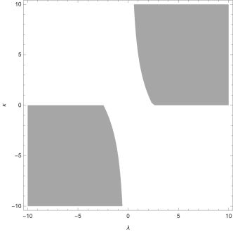
Figure 1: Region plot in the space $\left\{\lambda,\kappa\right\}$ where points $\mathbf{B=}\left(B_{1}^{\pm},B_{2}^{\pm}\right)$ are real.

The stationary points have the same physical properties, that is, the points describe universes with the same physical properties, where the physical quantities have the following values

$$w_{tot}\left(\mathbf{B}\right)=1-\frac{2\kappa}{\kappa+\lambda}~{},~{}w_{\phi}\left(\mathbf{B}\right)=-1+\frac{12}{6+\kappa\left(\kappa+\lambda\right)}~{},~{}w_{\psi}\left(\mathbf{B}\right)=1~{},$$ (35)

$$\Omega_{\phi}\left(\mathbf{B}\right)=1-\Omega_{\psi}\left(\mathbf{B}\right)~{},~{}\Omega_{\psi}\left(\mathbf{B}\right)=\left|\frac{\lambda\left(\kappa+\lambda\right)-6}{\left(\kappa+\lambda\right)^{2}}\right|.$$ (36)

From $w_{tot}\left(\mathbf{B}\right)$ it follows that the points describe scaling solutions and the de Sitter universe is recovered only when $\lambda=0$, which is excluded because for $\lambda=0$, the stationary points are not real. We continue by studying the stability of the stationary points. In Fig. 2, we present counter plots for the physical parameters $w_{tot}\left(\mathbf{B}\right),~{}w_{\phi}\left(\mathbf{B}\right)\,$ and $\Omega_{\psi}\left(\mathbf{B}\right)$ in the space of variables $\left\{\lambda,\kappa\right\}$.

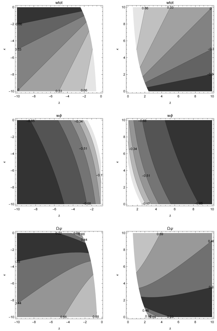
Figure 2: Qualitative evolution of the physical variables $w_{tot}\left(\mathbf{B}\right),~{}w_{\phi}\left(\mathbf{B}\right)\,$ and $\Omega_{\psi}\left(\mathbf{B}\right)$ of the exact solutions at the critical points $\mathbf{B=}\left(B_{1}^{\pm},B_{2}^{\pm}\right)$ for various values of the free variables $\left\{\lambda,\kappa\right\}$.

For the stationary points $B_{1}^{\pm}$ two of the five eigenvalues are expressed as

$$e_{1}\left(B_{1}^{\pm}\right)=3\frac{\kappa}{\kappa+\lambda},~{}e_{2}\left(B_{1}^{\pm}\right)=-3\frac{\kappa-\lambda}{\kappa+\lambda},$$

from where we observe that $e_{1}\left(B_{1}^{\pm}\right)>0$ in order for the points to be real, consequently the exact solutions at the stationary points $B_{1}^{\pm}$ are unstable.

We use the constraint $z^{2}=1-x^{2}-y^{2}-u^{2}$ such that the dynamical system is reduced by one-dimension. Thus, for the new four-dimensional system the eigenvalues of the linearized system around points $B_{1}^{\pm}$ are found

$$e_{1}\left(B_{1}^{\pm}\right) =3\frac{\kappa}{\kappa+\lambda},~{}e_{2}\left(B_{1}^{\pm}\right)=-3\frac{\kappa-\lambda}{\kappa+\lambda},$$

$$e_{3}\left(B_{1}^{\pm}\right) =-\frac{3\kappa+i\sqrt{3\kappa\left(4\lambda^{3}+8\kappa\lambda^{2}+4\left(\kappa^{2}-6\right)\lambda-27\kappa\right)}}{2\left(\kappa+\lambda\right)},$$

$$e_{4}\left(B_{1}^{\pm}\right) =-\frac{3\kappa-i\sqrt{3\kappa\left(4\lambda^{3}+8\kappa\lambda^{2}+4\left(\kappa^{2}-6\right)\lambda-27\kappa\right)}}{2\left(\kappa+\lambda\right)},$$

from where we conclude again that the exact scaling solutions at points $B_{1}^{\pm}$ are unstable. In particular points

Similarly, the eigenvalues of the linearized system around the points $B_{2}^{\pm}$ are calculated

$$e_{1}\left(B_{2}^{\pm}\right) =-3\frac{\kappa}{\kappa+\lambda},~{}e_{2}\left(B_{2}^{\pm}\right)=-3\frac{2\sigma\left(\kappa-\lambda\right)-\kappa}{2\sigma\left(\kappa+\lambda\right)},$$

$$e_{3}\left(B_{2}^{\pm}\right) =e_{3}\left(B_{1}^{\pm}\right),~{}e_{4}\left(B_{2}^{\pm}\right)=e_{3}\left(B_{1}^{\pm}\right),$$

Hence, we infer that the stationary points $B_{2}^{\pm}$  are attractors, and the exact solutions at the points are stable when the free parameters $\left\{\lambda,\kappa,\sigma\right\}$ are constraints as follows

$$\lambda\leq-\sqrt{6}:\left\{\kappa<\lambda,\sigma<0,\sigma>\frac{\kappa}{2\left(\kappa-\lambda\right)}\right\}\cup\left\{\kappa=\lambda,\sigma<0\right\}\cup\left\{\lambda<\kappa<0,\frac{\kappa}{2\left(\kappa-\lambda\right)}<\sigma<0\right\},$$

$$-\sqrt{6}<\lambda<-\sqrt{3}:\left\{\kappa<\lambda,\sigma<0,\sigma>\frac{\kappa}{2\left(\kappa-\lambda\right)}\right\}\cup\left\{\kappa=\lambda,\sigma<0\right\}\cup\left\{\lambda<\kappa<\frac{6-\lambda^{2}}{\lambda},\frac{\kappa}{2\left(\kappa-\lambda\right)}<\sigma<0\right\},$$

$$\lambda=-\sqrt{3}:\left\{\kappa<-\sqrt{3},~{}\sigma<0\right\}\cup\left\{\kappa<-\sqrt{3},~{}\frac{\kappa}{2\left(\sqrt{3}+\kappa\right)}<\sigma\right\},$$

$$-\sqrt{3}<\lambda<0:\left\{\kappa<\frac{6-\lambda^{2}}{\lambda},\sigma<0\right\}\cup\left\{\kappa<\frac{6-\lambda^{2}}{\lambda},\frac{\kappa}{2\left(\kappa-\lambda\right)}<\sigma\right\},$$

$$0<\lambda<\sqrt{3}:\left\{\kappa>\frac{6-\lambda^{2}}{\lambda},\sigma<0\right\}\cup\left\{\kappa>\frac{6-\lambda^{2}}{\lambda},\frac{\kappa}{2\left(\kappa-\lambda\right)}<\sigma\right\},$$

$$\lambda=\sqrt{3}:\left\{\kappa<\sqrt{3},~{}\sigma<0\right\}\cup\left\{\kappa<-\sqrt{3},~{}-\frac{\kappa}{2\left(\sqrt{3}-\kappa\right)}<\sigma\right\},$$

$$\sqrt{3}<\lambda<\sqrt{6}:\left\{\frac{6-\lambda^{2}}{\lambda}<\kappa<\lambda,\frac{\kappa}{2\left(\kappa-\lambda\right)}<\sigma<0\right\}\cup\left\{\kappa\geq\lambda,\sigma<0\right\}\cup\left\{\kappa>\lambda,\frac{\kappa}{2\left(\kappa-\lambda\right)}<\sigma\right\},$$

$$\lambda\geq\sqrt{6}:\left\{0<\kappa<\lambda,\frac{\kappa}{2\left(\kappa-\lambda\right)}<\sigma<0\right\}\cup\left\{\kappa\geq\lambda,\sigma<0\right\}\cup\left\{\kappa>\lambda,\frac{\kappa}{2\left(\kappa-\lambda\right)}<\sigma\right\}.$$

In Figs. 3 and 4 we plot the regions where the stationary points $B_{2}^{\pm}$ are attractors and the exact solutions on the stationary points points are stable.

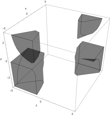
Figure 3: Region plot in the space of variabels $\left\{\kappa,\lambda,\sigma\right\}$ where the points $B_{2}^{\pm}$ are attractors.

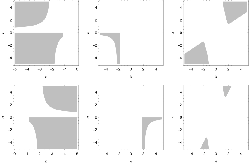
Figure 4: Region plots in the the planes $\kappa-\sigma,~{}\lambda-\sigma$ and $\lambda-\kappa$ where points $B_{2}^{\pm}$ are attractors. Left figures present the region in the plane $\kappa-\sigma$ for $\lambda=-2$ and $\lambda=2$; middle figures present the region in the plane $\lambda-\sigma$, for $\kappa=-2$ and $\kappa-2$ while right figures are in the plane for $\lambda-\kappa$ for $\sigma=-1$ and $\sigma=1$.

IV.3 Family C

The stationary points of Family C are two and they have coordinates

$$C_{1} =\left(-\frac{\kappa}{\sqrt{6}},0,0,\sqrt{1-\frac{\kappa^{2}}{6}},0\right),$$ (37)

$$C_{2} =\left(0,\sqrt{\frac{\kappa}{\kappa-\lambda}},0,\sqrt{\frac{\lambda}{\lambda-\kappa}},0\right).$$ (38)

Point $C_{1}$ is real when $\left|\kappa\right|\leq\sqrt{6}$ and the physical quantities of the exact solution at the point are

$$\left(w_{tot}\left(C_{1}\right),w_{\phi}\left(C_{1}\right),w_{\psi}\left(C_{1}\right),\Omega_{\phi}\left(C_{1}\right),\Omega_{\psi}\left(C_{1}\right)\right)=\left(-1+\frac{\kappa^{2}}{3},1,-1,\frac{\kappa^{2}}{6},1-\frac{\kappa^{2}}{6}\right).$$ (39)

Thus, stationary point $C_{1}$ describes a scaling solution. The scaling solution describes an accelerated universe when $\left|\kappa\right|<\sqrt{2}$.

Furthermore, the exact solution at the stationary point $C_{2}$ describes a de Sitter universe, where the two scalar fields mimic the cosmological constant, the physical quantities are

$$\left(w_{tot}\left(C_{2}\right),w_{\phi}\left(C_{2}\right),w_{\psi}\left(C_{2}\right),\Omega_{\phi}\left(C_{2}\right),\Omega_{\psi}\left(C_{2}\right)\right)=\left(-1,-1,-1,\frac{\kappa}{\kappa-\lambda},\frac{\lambda}{\lambda-\kappa}\right).$$ (40)

Point $C_{2}$ is real and physically accepted when $\lambda\kappa<0$, i.e. $\left\{\lambda<0,\kappa>0\right\}$ or $\left\{\lambda>0,\kappa<0\right\}$.

The linearized four-dimensional system around the stationary point $C_{1}$ admits the eigenvalues

$$e_{1}\left(C_{1}\right) =\frac{\kappa^{2}}{2},$$

$$e_{2}\left(C_{1}\right) =-\frac{1}{2}\left(6-\kappa^{2}\right)$$

$$e_{3}\left(C_{1}\right) =2\left(\kappa^{2}-3\right)$$

$$e_{4}\left(C_{1}\right) =\frac{1}{2}\kappa\left(\kappa-\lambda\right)$$

from where we infer that the exact solution at the stationary point is always unstable. Specifically, point $C_{1}$ is a saddle point.

For the stationary point $C_{2}$, we find that one of the eigenvalues of the linearized system around $C_{2}$ is zero. That eigenvalue corresponds to the linearize equation (24). As far as concerns the other three eigenvalues we plot numerically their values and we find that they have negative real parts for all the range of parameters $\left\{\lambda,\kappa\right\}$ where the point exists. In Fig. 5 we plot the real parts of the three nonzero eigenvalues of the linearized system. Therefore, we infer that the there exists a four-dimensional stable submanifold around the stationary point. However, because of the eigenvalues has zero real part the center manifold theorem (CMT) should be applied.

For simplicity on our calculations we apply the CMT for the five dimensional system. We find that the variables with nonzero real part on their eigenvalues, that is, variables $\left\{x,y,z,u\right\}$, according to the CMT theorem are approximated as functions of variable $\mu$ as follows

$$x =x_{00}\mu^{2}+x_{10}\mu^{3}+x_{20}\mu^{4}+O\left(\mu^{5}\right)~{},~{}y=y_{00}\mu^{2}+y_{10}\mu^{3}+y_{20}\mu^{4}+O\left(\mu^{5}\right),~{}$$

$$z =z_{00}\mu^{2}+z_{10}\mu^{3}+z_{20}\mu^{4}+O\left(\mu^{5}\right)~{},~{}u=u_{00}\mu^{2}+u_{10}\mu^{3}+u_{20}\mu^{4}+O\left(\mu^{5}\right)$$

where $\left\{x_{00},y_{00},z_{00},u_{00}\right\}=\left(0,0,z_{00},0\right)$; $x_{10}=-\frac{z_{00}}{\kappa},~{}y_{10}=\sqrt{\frac{3}{2}}\frac{z_{00}}{\sqrt{\kappa^{3}\left(\kappa-\lambda\right)}},~{}$etc.

Hence, the fifth equation, i.e. equation (20) is written $\frac{d\mu}{d\tau}=\alpha\mu^{4}+a_{1}\mu^{5}+O\left(\mu^{6}\right)~{}$where $\alpha=\frac{\sqrt{6}\left(\kappa\lambda-2\left(\kappa\lambda+3\right)\sigma\right)}{2\kappa\lambda+6}z_{00}-\frac{6\kappa\left(\sqrt{\lambda\left(\lambda-\kappa\right)}\right)}{2\kappa\lambda+6}u_{10}$. Therefore, the point is always unstable for $a\neq 0$, however from the coefficient term $a_{1}\mu^{5}$ we find that the point can be stable.

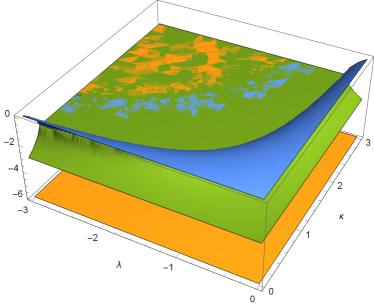
Figure 5: Qualitative evolution for the real parts of the nonzero eigenvalues of the linearized system around the stationary point $C_{2}$.

IV.4 Family D

The fourth family of stationary points is consists of the following six stationary points

$$D_{1}^{\pm}=\left(-\sqrt{\frac{3}{2}}\frac{1}{\kappa},0,\pm\frac{\sqrt{\kappa^{2}-3}}{\sqrt{2}\kappa},\frac{1}{\sqrt{2}},0\right),$$ (41)

$$D_{2}^{\pm}=\left(x_{D_{2}},0,\pm z_{D_{2}},\sqrt{1-\left(x_{D_{2}}\right)^{2}-\left(z_{D_{2}}\right)^{2}},\mu_{D_{2}}\right),$$ (42)

$$D_{3}^{\pm}=\left(x_{D_{3}},0,\pm z_{D3},\sqrt{1-\left(x_{D_{3}}\right)^{2}-\left(z_{D_{3}}\right)^{2}},\mu_{D_{3}}\right),$$ (43)

with

$$x_{D_{2}} =-\frac{\kappa^{2}(2\sigma-1)+\sqrt{-4\kappa^{4}\sigma+\kappa^{4}+4\left(\kappa^{2}-3\right)^{2}\sigma^{2}}+6\sigma}{\sqrt{6}\kappa(4\sigma-1)},$$

$$z_{D_{2}} =\frac{\sqrt{-\kappa^{4}(1-2\sigma)^{2}+6\kappa^{2}\sigma\left(8\sigma^{2}-2\sigma+1\right)-\sqrt{-4\kappa^{4}\sigma+\kappa^{4}+4\left(\kappa^{2}-3\right)^{2}\sigma^{2}}\left(\kappa^{2}(2\sigma-1)+24\sigma^{2}\right)-144\sigma^{3}}}{2\sqrt{3}\kappa\sqrt{\sigma}(4\sigma-1)},$$

$$\mu_{D_{2}} =z_{D_{2}}\frac{\sqrt{6}\left(\kappa^{2}(1-2\sigma)^{2}+2\sigma\left(\sqrt{-4\kappa^{4}\sigma+\kappa^{4}+4\left(\kappa^{2}-3\right)^{2}\sigma^{2}}-6\sigma\right)\right)}{\kappa^{2}(1-2\sigma)^{2}-24\sigma^{2}},$$

$$x_{D_{3}} =\frac{\kappa^{2}(1-2\sigma)+\sqrt{-4\kappa^{4}\sigma+\kappa^{4}+4\left(\kappa^{2}-3\right)^{2}\sigma^{2}}-6\sigma}{\sqrt{6}\kappa(4\sigma-1)},$$

$$z_{D_{3}} =\frac{\sqrt{-\kappa^{4}(1-2\sigma)^{2}+6\kappa^{2}\sigma\left(8\sigma^{2}-2\sigma+1\right)+\sqrt{-4\kappa^{4}\sigma+\kappa^{4}+4\left(\kappa^{2}-3\right)^{2}\sigma^{2}}\left(\kappa^{2}(2\sigma-1)+24\sigma^{2}\right)-144\sigma^{3}}}{2\sqrt{3}\kappa\sqrt{\sigma}(4\sigma-1)},$$

$$\mu_{D_{3}} =z_{D_{3}}\frac{\sqrt{6}\left(2\sigma\left(\sqrt{-4\kappa^{4}\sigma+\kappa^{4}+4\left(\kappa^{2}-3\right)^{2}\sigma^{2}}+6\sigma\right)-\kappa^{2}(1-2\sigma)^{2}\right)}{\kappa^{2}(1-2\sigma)^{2}-24\sigma^{2}}\text{. }$$

Points $D_{1}^{\pm}$ describe a scaling solution where the effective fluid is pressureless, that is, it describes a dust fluid source and the scale factor is $a\left(t\right)=a_{0}t^{\frac{2}{3}}$. The physical parameters of the exact solution at points $D_{1}^{\pm}$ are

$$w_{tot}\left(D_{1}^{\pm}\right)=0~{},~{}w_{\phi}\left(D_{1}^{\pm}\right)=1~{},~{}w_{\psi}\left(D_{1}^{\pm}\right)=\frac{3}{3-2\kappa^{2}}~{},$$ (44)

$$\Omega_{\phi}\left(D_{1}^{\pm}\right)=\frac{3}{2\kappa^{2}}~{},~{}\Omega_{\psi}\left(D_{1}^{\pm}\right)=1-\frac{3}{2\kappa^{2}}.$$ (45)

Remark that points $D_{1}^{\pm}$ are real when $\left|\kappa\right|>\sqrt{3}$. The eigenvalues of the four-dimensional linearized system around the stationary points $D_{1}^{\pm}$ are derived

$$e_{1}\left(D_{1}^{\pm}\right) =\frac{3}{2}$$

$$e_{2}\left(D_{1}^{\pm}\right) =\frac{3}{2}\left(\kappa-\lambda\right)$$

$$e_{3}\left(D_{1}^{\pm}\right) =-\frac{3+\sqrt{3\left(51-16\kappa^{2}\right)}}{4}$$

$$e_{4}\left(D_{1}^{\pm}\right) =-\frac{3-\sqrt{3\left(51-16\kappa^{2}\right)}}{4}$$

from where we infer that the stationary points $D_{1}^{\pm}$ are always unstable. Points $D_{1}^{\pm}$   are saddle points.

Points $D_{2}^{\pm}$ are real and physically accepted when $\left\{\sigma\in\left(0,\frac{1}{4}\right)\cup\left(\frac{1}{4},\frac{1}{2}\right),\kappa>\frac{2\sqrt{6}\sigma}{2\sigma-1}\right\}\cup\left\{\frac{2\sqrt{6}\sigma}{1-2\sigma}<\kappa<-\sqrt{6}\sqrt{\frac{2\sigma^{2}+\sigma\sqrt{4\sigma-1}}{\left(1-2\sigma\right)^{2}}},\sigma>\frac{1}{2}\right\}$ and $\left\{\kappa<0,\sigma\,<0\right\}$ as they are presented in Fig. 6. The exact solution at the stationary points describe a scaling solution with values of the equation of state parameter $w_{tot}\left(\kappa,\sigma\right)$ as they presented in Fig. 6. For the linearized four-dimensional system one of the eigenvalues is

$$e_{1}\left(D_{2}^{\pm}\right)=\frac{A\left(\kappa,\sigma\right)(2\kappa\sigma-\kappa-2\lambda\sigma)}{4\kappa\sigma(4\sigma-1)\left(2\kappa^{2}\sigma-\kappa^{2}+24\sigma^{2}\right)},$$

where

$$A\left(\kappa,\sigma\right) =4\kappa^{4}\sigma^{2}-4\kappa^{4}\sigma+\kappa^{4}+48\kappa^{2}\sigma^{3}-12\kappa^{2}\sigma^{2}-6\kappa^{2}\sigma$$

$$+\sqrt{\left(2\kappa^{2}\sigma-\kappa^{2}+24\sigma^{2}\right)^{2}\left(4\kappa^{4}\sigma^{2}-4\kappa^{4}\sigma+\kappa^{4}-24\kappa^{2}\sigma^{2}+36\sigma^{2}\right)}+144\sigma^{3}.$$

The other three eigenvalues are only functions of $\kappa,\sigma$, that is $e_{2,3,4}\left(D_{2}^{\pm}\right)=e_{2,3,4}\left(\kappa,\sigma\right)$. Numerically, we find that there are not any values of $\left\{\kappa,\sigma\right\}$ where the points $D_{2}^{\pm}$ are defined, such that all the eigenvalues have real part negative, consequently, the stationary points are always sources and the exact solutions at the stationary points $D_{2}^{\pm}$ are always unstable.

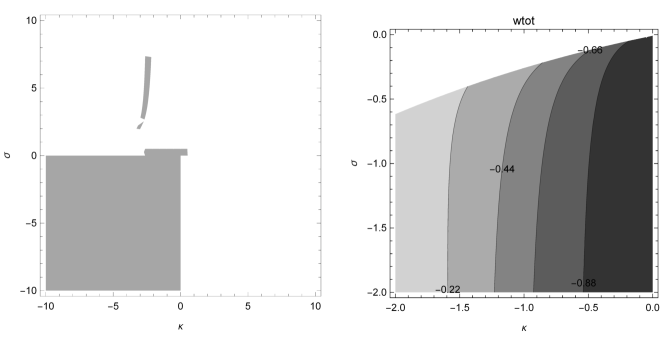
Figure 6: Left figure: Region plot in the space $\left\{\kappa,\sigma\right\}$ where points $D_{2}^{\pm}$ are real and physical accepted. Right Figure: Contour plot of the equation of state parameter for the effective fluid $w_{tot}\left(\kappa,\sigma\right)$ at the critical points $D_{2}^{\pm}$.

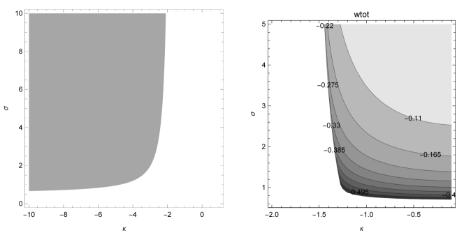
Figure 7: Left figure: Region plot in the space $\left\{\kappa,\sigma\right\}$ where points $D_{3}^{\pm}$ are real and physical accepted. Right Figure: Contour plot of the equation of state parameter for the effective fluid $w_{tot}\left(\kappa,\sigma\right)$ at the critical points $D_{3}^{\pm}$.

Stationary points $D_{3}^{\pm}$ have similar physical properties with points $D_{2}^{\pm}$, indeed they describe scaling solutions only. The points are real and physically accepted in the region $\left\{\sigma>\frac{1}{2},\kappa<-\sqrt{\frac{6\sigma}{\sqrt{4\sigma-1}-2\sigma}}\right\}$.

In Fig. 7 we present the region in the space $\left\{\sigma,\kappa\right\}$ where the points are defined as also the counter plot of the equation of state parameter for the effective fluid source which describes the exact solution at the points $D_{3}^{\pm}$. In a similar way with points $D_{2}^{\pm}$ we find that there is not any range in the space $\left\{\kappa,\sigma\right\}$ where the points are attractors. Consequently, the stationary points $D_{3}^{\pm}$   are sources. The main physical results of the stationary points are summarized in Table 1.

Table 1: The physical propreties of the stationary models in chiral cosmology

Point	Contribution of $\phi$	Contribution of $\psi$	Scaling/de Sitter	Possible $w_{tot}<-\frac{1}{3}$	Stability
$A_{1}$	Yes only kinetic part	No	Scaling	No	Unstable
$A_{2}$	Yes	No	Scaling	Yes	Unstable
$B_{1}^{\pm}$	Yes	Yes only kinetic part	Scaling	Yes	Unstable
$B_{2}^{\pm}$	Yes	Yes only kinetic part	Scaling	Yes	Can be Stable
$C_{1}$	Yes only kinetic	Yes only potential	Scaling	Yes	Unstable
$C_{2}$	Yes only potential	Yes only potential	de Sitter $\left(w_{tot}=-1\right)$	Always	CMT
$D_{1}^{\pm}$	Yes	Yes	Scaling $\left(w_{tot}=0\right)$	No	Unstable
$D_{2}^{\pm}$	Yes	Yes	Scaling	Yes	Unstable
$D_{3}^{\pm}$	Yes	Yes	Scaling	Yes	Unstable

V Application $\left(\kappa,\sigma\right)=\left(2,\frac{1}{2}\right)$

Consider now the case where $\kappa=2$ and $\sigma=\frac{1}{2}$, while $\lambda$ is an arbitrary constant. For that consideration, the stationary points of the dynamical system (20)-(24) have the following coordinates

$$\bar{A}_{1}^{\pm} =\left(\pm 1,0,0,0,0\right),~{}$$

$$\bar{A}_{2} =\left(-\frac{\lambda}{\sqrt{6}},\sqrt{1-\frac{\lambda^{2}}{6}},0,0,0\right),$$

$$\bar{B}_{1}^{\pm} =\left(-\frac{\sqrt{6}}{\lambda+2},\sqrt{\frac{2}{\lambda+2}},\pm\sqrt{\frac{\left(\lambda+1\right)^{2}-7}{\left(\lambda+2\right)^{2}}},0,0\right),~{}$$

$$\bar{B}_{2}^{\pm} =\left(-\frac{\sqrt{6}}{\lambda+2},\sqrt{\frac{2}{\lambda+2}},\sqrt{\frac{\left(\lambda+1\right)^{2}-7}{\left(\lambda+2\right)^{2}}},0,2\sqrt{\frac{6}{\left(\lambda+1\right)^{2}-7}}\right),$$

$$\bar{C}_{1} =\left(-\sqrt{\frac{2}{3}},0,0,\frac{1}{\sqrt{3}},0\right),~{}$$

$$\bar{C}_{2} =\left(0,\left(1-\frac{\lambda}{2}\right)^{-1},0,\sqrt{\frac{\lambda}{\lambda-2}}\right),$$

$$\bar{D}_{1}^{\pm} =\left(-\frac{1}{2}\sqrt{\frac{3}{2}},0,\frac{1}{2\sqrt{2}},\frac{1}{\sqrt{2}},0\right).$$

Points $\bar{A}_{1}^{\pm},~{}\bar{A}_{2}$ are sources and since they do not depend on the parameters $\kappa,\sigma$ their physical properties are the same as before. Recall that point $\bar{A}_{2}$ is real for $\left|\lambda\right|<\sqrt{6}$. Stationary points $\mathbf{B}=\left(\bar{B}_{1}^{\pm},\bar{B}_{2}^{\pm}\right)$ exist when $\lambda>\sqrt{7}-1$. The physical parameters at the points are simplified as follows

$$w_{tot}\left(\mathbf{B}\right)=\frac{\lambda-2}{\lambda+2}~{},~{}w_{\phi}\left(\mathbf{B}\right)=-1+\frac{6}{5\lambda}~{},~{}w_{\psi}\left(\mathbf{B}\right)=1~{},$$ (46)

$$\Omega_{\phi}\left(\mathbf{B}\right)=\frac{2\left(\lambda+5\right)}{\left(\lambda+2\right)^{2}}~{},~{}\Omega_{\psi}\left(\mathbf{B}\right)=1-\frac{2\left(\lambda+5\right)}{\left(\lambda+2\right)^{2}}.$$ (47)

The exact solutions at points $\bar{B}_{1}^{\pm}$ are always unstable. However, for points $\bar{B}_{2}^{\pm}$ we find that $e_{2}\left(\bar{B}_{2}^{\pm}\right)>0$ for $\lambda>\sqrt{7}-1$ which means that points $\bar{B}_{2}^{\pm}$ are sources. The parameter for the equation of state $w_{tot}\left(\mathbf{B}\right)$ is constraint as $\frac{\sqrt{7}-3}{\sqrt{7+1}}<w_{tot}\left(B\right)<1$, while for $\lambda=2$, $w_{tot}\left(\mathbf{B}\right)=0$ the exact solutions have the scale factor $a\left(t\right)=a_{0}t^{\frac{2}{3}}$,   while for $\lambda=4$, $w_{tot}\left(\mathbf{B}\right)=\frac{1}{3}$, that is $a\left(t\right)=a_{0}t^{\frac{1}{2}}$.

Furthermore, stationary point $\bar{C}_{1}$ is a source and describes the radiation epoch, $w_{tot}\left(\bar{C}_{1}\right)=\frac{1}{3}$, on the other hand, at point $\bar{C}_{2}$ the exact solution is that of de Sitter universe, the point is real for $\lambda<0\mathbf{.}$Finally, points $\bar{D}_{1}^{\pm}$ points describe the unstable scaling solutions which describe the matter dominated era, that is, $w_{tot}\left(\bar{D}_{1}^{\pm}\right)=0$.

In Figs. 8 and 9, the evolution of the physical variables $\left\{w_{tot},w_{\phi},w_{\psi},\Omega_{\phi},\Omega_{\psi}\right\}$ is presented for the specific model for $\lambda=-4$ and $\lambda=-2$ and for different initial conditions for the integration of the dynamical system (20)-(24). Recall that the de Sitter point $\bar{C}_{2}$ is a source; however, it admits a four-dimensional stable manifold when $\mu\rightarrow 0$. We observe that in the de Sitter point the physical parameters $\Omega_{\phi},~{}\Omega_{\psi}$ are not zero which means that the all the parts of the potential $V\left(\phi,\psi\right)$ contributes to the cosmological fluid. The initial conditions have been considered such that to describe a wide range of solutions and different behaviour. The large number of stationary points is observed from the behaviour of $w_{tot}$, which has various maxima before reach the de Sitter point. Similarly from the diagram of $\left\{\Omega_{\phi},~{}\Omega_{\psi}\right\}$, we observe that there is a alternation between the domination of the two fields.

Figure 8: Evolution of the physical variables $\left\{w_{tot},w_{\phi},w_{\psi},\Omega_{\phi},\Omega_{\psi}\right\}$ for numerical solutions of the field equations with $\kappa=2,~{}\sigma=\frac{1}{2}$ and $\lambda=-4$. The plots are for different initial conditions $\left(x\left(0\right),y\left(0\right),z\left(0\right),u\left(0\right),\mu\left(0\right)\right)$ where $\mu\left(0\right)$ has been chosen to be near to zero, such that the de Sitter point $\bar{C}_{2}$ to be an attractor.

Figure 9: Evolution of the physical variables $\left\{w_{tot},w_{\phi},w_{\psi},\Omega_{\phi},\Omega_{\psi}\right\}$ for numerical solutions of the field equations with $\kappa=2,~{}\sigma=\frac{1}{2}$ and $\lambda=-2$. The plots are for different initial conditions $\left(x\left(0\right),y\left(0\right),z\left(0\right),u\left(0\right),\mu\left(0\right)\right)$ where $\mu\left(0\right)$ has been chosen to be near to zero, such that the de Sitter point $\bar{C}_{2}$ to be an attractor.

Consider now the cosmographic parameters $q,~{}j$ and $s$ which are defined as cowei

$$q\left(x,y,z,u,\mu;\lambda,\kappa,\sigma\right)=-1-\frac{\dot{H}}{H^{2}}$$ (48)

$$j\left(x,y,z,u,\mu;\lambda,\kappa,\sigma\right)=\frac{\ddot{H}}{H^{3}}-3q-2$$ (49)

$$s\left(x,y,z,u,\mu;\lambda,\kappa,\sigma\right)=\frac{H^{\left(3\right)}}{H^{4}}+4j+3q(q+4)+6$$ (50)

In Fig. 10 we present the evolution of the cosmographic parameters for the application we considered in this example as also for additional values of the free parameters $\left\{\lambda,\kappa,\sigma\right\}$, while all the plots are for the same initial conditions. Here we present the qualitative evolution of these parameters, however the cosmographic parameters as also the free parameters of the theory can be constrained by the observations cob1 .

Figure 10: Qualitative evolution of the cosmographic parameters $\left\{q,j,s\right\}$ for various values of the free parameters $\left\{\lambda,\kappa,\sigma\right\}$. The plots of the first row are for $\left\{\lambda,\kappa,\sigma\right\}=\left\{-4,\pm 2,\frac{1}{2}\right\}$  while the plots of the second row are for $\left\{\lambda,\kappa,\sigma\right\}=\left\{-2,\pm 2,\frac{1}{2}\right\}$.  From the figure we observe that in order the future attractor to be a de Sitter point then $\kappa>0.$

In the following section we continue our analysis by presenting analytic solutions for the model of our study.

VI Analytic solution

We consider the point-like Lagrangian

$$\mathcal{L}\left(a,\dot{a},\phi,\dot{\phi},\psi,\dot{\psi}\right)=-3a\dot{a}^{2}+\frac{1}{2}a^{3}\left(\dot{\phi}^{2}+e^{\kappa\phi}\dot{\psi}^{2}\right)-a^{3}\left(V_{0}e^{\lambda\phi}+U_{0}\psi^{\frac{1}{\sigma}}e^{\kappa\phi}\right).$$ (51)

Analytic solutions of form of Lagrangian (51) were presented before in 2sfand . By using the results and the analysis of 2sfand we present an analytic solutions for specific values of the parameters $\left\{\lambda,\kappa,\sigma\right\}$ in order to support the results of the previous section. Specifically for the free variables we select $\left(\lambda,\kappa,\sigma\right)=\left(-\frac{\sqrt{6}}{2},-\frac{\sqrt{6}}{2},\frac{1}{2}\right)$. These values are not random. In particular, from the results of 2sfand it follows that for these specific values the field equations admit conservation laws and they form a Liouville integrable dynamical system, such that the field equations can be solved by quadratures.

In order to simplify the field equations and write the analytic solution by using closed-form functions, we apply the point transformation

$$a=\left(xz-\frac{3}{8}y^{2}\right)^{\frac{1}{3}}~{},~{}\phi=-2\sqrt{\frac{2}{3}}\ln\left(\frac{x}{\sqrt{\left(xz-\frac{3}{8}y^{2}\right)}}\right)~{},~{}\psi=\frac{y}{x}$$ (52)

such that Lagrangian (51) is written as

$$\mathcal{L}\left(x,\dot{x},y,\dot{y},z,\dot{z}\right)=-\frac{4}{3}\dot{x}\dot{z}-V_{0}x^{2}+\frac{1}{2}\dot{y}^{2}-U_{0}y^{2}.$$ (53)

In the new coordinates the field equations are

$$\ddot{x}=0~{},~{}\ddot{y}+2U_{0}y=0~{},~{}\ddot{z}-\frac{3}{2}V_{0}x=0,$$ (54)

with constraint equation

$$-\frac{4}{3}\dot{x}\dot{z}+V_{0}x^{2}+\frac{1}{2}\dot{y}^{2}+U_{0}y^{2}=0.$$ (55)

Easily, we find the exact solution

$$x=x_{1}t+x_{0}~{},~{}z=\frac{1}{4}V_{0}x_{1}t^{3}+\frac{3}{4}V_{0}x_{0}t^{2}+z_{1}t+z_{0}~{},$$ (56)

$$y\left(t\right)=y_{1}\cos\left(\sqrt{2U_{0}}t\right)+y_{2}\sin\left(\sqrt{2U_{0}}t\right)$$ (57)

with constraint condition $V_{0}x_{0}^{2}-\frac{4}{3}x_{1}z_{1}+U_{0}\left(y_{1}^{2}+y_{2}^{2}\right)$.  For $x_{0}=z_{0}=y_{1}=0$, the scale factor is written $a\left(t\right)=\left(\frac{x_{1}}{4}V_{0}t^{4}+x_{1}z_{1}t^{2}-\frac{3}{8}\left(y_{2}\right)^{2}\sin\left(\sqrt{2U_{0}}t\right)\right)^{\frac{1}{3}}.$ It is easy to observe that the present analytic solution does not provide any de Sitter point. That is in agreement with the result of the previous section, since for $\lambda=\kappa$, the de Sitter point $C_{2}$ does not exist. For more general solutions with expansion eras and de Sitter phases we refer the reader to 2sfand .

VII With a matter source

Let us assume now the presence of an additional pressureless matter source in field equations with energy density $\rho_{m}$ and let us discuss the existence of additional stationary points. For a pressureless fluid source the dimensionless field equations (20)-(25) remain the same, while the constraint equation (28) becomes

$$\Omega_{m}=1-x^{2}-y^{2}-z^{2}-u^{2}$$ (58)

where $\Omega_{m}=\frac{\rho_{m}}{3H^{2}}$, and $0\leq\Omega_{m}\leq 1$.

For this model, the stationary points found before exist and give $\Omega_{m}=0$, while when $\Omega_{m}\neq 0$ the additional points exist

$$E_{1}=\left(-\sqrt{\frac{3}{2}}\frac{1}{\lambda},\sqrt{\frac{3}{2}}\frac{1}{\lambda},0,0,0\right)~{},~{}E_{2}=\left(-\sqrt{\frac{3}{2}}\frac{1}{\kappa},0,0,\sqrt{\frac{3}{2}}\frac{1}{\kappa},0\right)$$ (59)

$$E_{3}=\left(-\sqrt{\frac{3}{2}}\frac{1}{\kappa},0,z,\sqrt{\frac{3}{2}+\kappa^{2}z^{2}}\frac{1}{\kappa},0\right)$$ (60)

Point $E_{1}$ is physically accepted when $\left|\lambda\right|>\sqrt{\frac{3}{2}}$ and describes the tracking solution with $\Omega_{m}\left(E_{1}\right)=1-\frac{3}{\lambda^{2}}$ where the field $\phi$ mimics the ideal gas $\rho_{m},~{}$that is, $w_{\phi}\left(E_{1}\right)=0,$ while the second field $\psi$ does not contribute, i.e. $z\left(E_{1}\right)=u\left(E_{1}\right)=0$.

For $E_{2}$ we find $\left(w_{tot}\left(E_{2}\right),w_{\phi}\left(E_{2}\right),w_{\psi}\left(E_{2}\right),\Omega_{\phi}\left(E_{2}\right),\Omega_{\psi}\left(E_{2}\right)\right)=\left(0,1,-1,\frac{3}{2\kappa^{2}},\frac{3}{2\kappa^{2}}\right)$, which means that it is another tracking tracking solution with $\Omega_{m}=1-\frac{3}{\kappa^{2}}$; the point is physically accepted when $\left|\kappa\right|\geq\sqrt{\frac{3}{2}}$.

$E_{3}$ does not describe one point, but a family of points on the surface $u\left(z\right)=$ $\sqrt{\frac{3}{2}+\kappa^{2}z^{2}}$ , for $x\left(E_{3}\right)=-\sqrt{\frac{3}{2}}\frac{1}{\kappa},$ $y\left(E_{3}\right)=\mu\left(E_{3}\right)=0$. It describes a tracking solution, that is $w_{tot}\left(E_{3}\right)=0$, with physical parameters

$$\left(w_{tot}\left(E_{3}\right),w_{\phi}\left(E_{3}\right),w_{\psi}\left(E_{3}\right),\Omega_{\phi}\left(E_{3}\right),\Omega_{\psi}\left(E_{3}\right)\right)=\left(0,1,-\frac{3}{4+3\kappa^{2}z^{2}},\frac{3}{2\kappa^{2}},2z^{2}+\frac{3}{2\kappa^{2}}\right),$$ (61)

while the point is physically accepted when  $\left|\kappa\right|\geq\sqrt{\frac{3}{2}}$ and $\left|z\right|\leq\frac{1}{2}\sqrt{2-\frac{3}{\kappa^{2}}}$. When $z\left(E_{3}\right)=0$, then $E_{3}$ reduces to $E_{2}$. What it is important, to mention is that the stability analysis for all the previous points changes, since we made use of the constraint equation (28).

VIII Conclusions

In this work we performed a detailed study of the dynamics for a two scalar field model with a mixed potential term known as Chiral model. The purpose of our analysis was to study the cosmological evolution of that specific model as also the cosmological viability of the model and which epochs of the cosmological evolution can be described by the Chiral model.

For the scalar field potential we assumed that it is of the form $V\left(\phi,\psi\right)=V_{0}e^{\lambda\phi}+U_{0}\psi^{\frac{1}{\sigma}}e^{\kappa\phi}$. For this consideration and without assuming the existence of additional matter source, we found four families of stationary points which provide nine different cosmological solutions. Eight of the cosmological solutions are scaling solutions which describe spacetimes with a a perfect fluid with a constant equation of state parameter $w\left(P\right)$. One of the scaling solutions describes a universe with a stiff matter, $w\left(P\right)=1$, another scaling solution correspond to a universe with a pressureless fluid source, $w\left(P\right)=0$, while for the rest six scaling solutions $w\left(P\right)=w\left(P,\lambda,\kappa,\sigma\right)$, which can describe accelerated eras for for specific values of the free parameters $\left\{\lambda,\kappa,\sigma\right\}$. Moreover, the ninth exact cosmological solution which was found from the analysis of the stationary points describes a de Sitter universe.

As far as the stability of the exact solutions at the stationary points is concerned, seven of the points are always unstable. while only the set of the points $B_{2}^{\pm}~{}$can be stable. Point $C_{2}$ which describes the de Sitter universe, has one eigenvalue negative while the rest of the eigenvalues are always negative. Consequently, according to the center manifold theorem we found the internal surface where the point $C_{2}$ is a source. Moreover, in the presence of additional matter source only additional tracking solutions follow, similarly to the quintessence model.

From the above results we observe that the specific Chiral cosmological model can describe the major eras of the cosmological history, that is, the late expansion era, an unstable matter dominated era, and two scaling solutions describe the radiation dominated era and the early acceleration epoch, therefore, the model in terms of dynamics it is cosmologically viable.

From this analysis it is clear that the Chiral cosmological model can be used as dark energy candidate. In a future work we plan to apply the cosmological observations to constrain the theory.

References

- (1) A. G. Riess, et al., Astron J. 116, 1009 (1998)
- (2) S. Perlmutter, et al., Astrophys. J. 517, 565 (1998)
- (3) P. Astier et al., Astrophys. J. 659, 98 (2007)
- (4) N. Suzuki et al., Astrophys. J. 746, 85 (2012)
- (5) G. Hinshaw et al. [WMAP Collaboration], Astrophys. J. Suppl. 208, 19 (2013)
- (6) P. A. R. Ade et al. [Planck Collaboration], Astron. Astrophys. 594, A13 (2016)
- (7) A. Guth, Phys. Rev. D 23, 347 (1981)
- (8) B. Ratra and P.J.E. Peebles, Phys. Rev. D 37, 3406 (1988)
- (9) G.W. Hordenski, Int. J. Theor. Phys. 10, 363 (1975)
- (10) C. Deffayet, G. Esposito-Farese and A. Vikman, Phys. Rev. D 79, 084003 (2009)
- (11) A.A. Coley and R.J. van den Hoogen, Phys. Rev. D 62, 023517 (2000)
- (12) T. Clifton, P.G. Ferreira, A. Padilla and C. Skordis, Phys. Rept. 513, 1 (2012)
- (13) J. Klusoň, Class. Quantum Grav. 28, 125025 (2011)
- (14) D. Sáez-Gómez, Phys. Rev. D 85, 023009 (2012)
- (15) J.D. Barrow and A.A.H. Graham, Phys. Rev. D 91, 083513 (2015)
- (16) D.N. Page, Class. Quant. Grav. 1, 417 (1984)
- (17) S. Basilakos and G. Luke-Gerakopoulos, Phys. Rev. D 78, 083509 (2008)
- (18) J.D. Barrow, Phys. Rev. D 48, 1585 (1993)
- (19) A. Muslimov, Class. Quant. Grav. 7, 231 (1990)
- (20) G.F.R. Ellis and M.S. Madsen, Class. Quant. Grav. 8, 667 (1991)
- (21) J.D. Barrow and P. Saich, Class. Quant. Grav. 10, 279 (1993)
- (22) R. de Ritis, G. Marmo, G. Platania, C. Rubano, P. Scudellaro and C. Stornaiolo, Phys. Rev. D. 42 1091 (1990)
- (23) S. Basilakos, M. Tsamparlis and A. Paliathanasis, Phys. Rev. D 83, 103512 (2011)
- (24) J.D. Barrow and A. Paliathanasis, Phys. Rev. D 94, 083518 (2016)
- (25) E.J. Copeland, M. Sami and S. Tsujikawa, IJMPD 15, 1753 (2006)
- (26) G. Leon and F.O. Franz Silva, Generalized scalar field cosmologies, arXiv:1912.09856
- (27) V. Faraoni, Cosmology in Scalar-Tensor Gravity, Springer, Dordrecht (2004)
- (28) V. Sivanesan, Phys. Rev. D 90, 104006 (2014)
- (29) V. Gorini, A. Yu. Kamenshchik, U. Moschella and V. Pasquier, Phys. Rev. D 69, 123512 (2004)
- (30) N. Chow and J. Khoury, Phys. Rev. D 80, 024037 (2009)
- (31) G. Leon and E.N. Saridakis, JCAP 1303, 025 (2013)
- (32) L.P. Chimento, M. Forte, R. Lazkoz and M.G. Richarte, Phys. Rev. D 043502 (2009)
- (33) J. Socorro and E.O. Nunez, Eur. Phys. J. Plus 132, 168 (2017)
- (34) A. Giacomini, G. Leon, A. Paliathanais and S. Pan, EPJC 80, 184 (2020)
- (35) A. Paliathanasis, Gen. Rel. Grav. 51, 101 (2019)
- (36) D. Benisty and E.I. Guendelman, Class. Quantum Grav. 36, 095001 (2019)
- (37) A.D. Lindle, Phys. Rev. D 49, 784 (1994)
- (38) E.J. Copeland, A.R. Liddle, D.H. Lyth, E.W. Steward and D. Wands, Phys. Rev. D 49, 6410 (1994)
- (39) S.A. Kim and A.R. Liddle, Phys. Rev. D 74, 023513 (2006)
- (40) D. Wands, Lect. Notes Phys. 738, 275 (2008)
- (41) P. Carrilho, D. Mulryne, J. Ronaye and T. Tenkanen, JCAP 06, 032 (2018)
- (42) P. Christodoulidis, D. Roest and E.I. Sfakianakis, JCAP 11, 002 (2019)
- (43) W. Hu, Phys. Rev. D 71, 047301 (2005)
- (44) Y.-F. Cai, E.N. Saridakis, M.R. Setare and J.-Q. Xia, Phys. Rept. 493, 1 (2010)
- (45) R. Lazkoz, G. Leon and I. Quiros, Phys. Lett. B 649, 103 (2007)
- (46) S.V. Chervon, Quantum Matter 2, 71 (2013)
- (47) I.V. Fomin, J. Phys.: Conf. Ser. 918, 012009 (2017)
- (48) S. V. Ketov, Quantum Non-linear Sigma Models, Springer-Verlag, Berlin, (2000).
- (49) N. Dimakis, A. Paliathanasis, P.A. Terzis and T. Christodoulakis, EPJC 79, 618 (2019)
- (50) P. Christodoulidis, D. Roest and E.I. Sfakianakis, JCAP 12, 059 (2019)
- (51) A. Paliathanasis and M. Tsamparlis, Phys. Rev. D 90, 043529 (2014)
- (52) L. Amendola, G. Camargo Campos and R. Rosenfeld, Phys. Rev. D 75, 083506 (2007)
- (53) D. Pavón and B. Wang, Gen. Rel. Grav. 41, 1 (2009)
- (54) L. P. Chimento, Phys. Rev. D 81, 043525 (2010)
- (55) F. Arevalo, A. P. R. Bacalhau and W. Zimdahl, Class. Quant. Grav. 29, 235001 (2012)
- (56) A. Paliathanasis, S. Pan and W. Yang, IJMPD 28, 1950161 (2019)
- (57) G. Papagiannopoulos, P. Tsiami, S. Basilakos and A. Paliathanasis, EPJC 80, 55 (2020)
- (58) D. Begue, C. Stahl and S.-S. Xue, Nucl. Phys. B 940, 312 (2019)
- (59) M. Szydlowski, T. Stachowiak and R. Wojtak, Phys. Rev. D 73, 063516 (2006)
- (60) W. Yang, S. Pan and A. Paliathanasis, MNRAS 482, 1007 (2019)
- (61) S. Pan, W. Yang and A. Paliathanasis, to appear in MNRAS (DOI:10.1093/mnras/staa213) (2020)
- (62) L. Amendola, D. Polarski and S. Tsujikawa, IJMPD 16, 1555 (2007)
- (63) G. Leon and E.N. Saridakis, JCAP 1504, 031 (2015)
- (64) G. Leon, IJMPE 20, 19 (2011)
- (65) T. Gonzales, G. Leon and I. Quiros, Class. Quantum Grav. 23, 3165 (2006)
- (66) A. Giacomini, S. Jamal, G. Leon, A. Paliathanasis and J. Saveedra, Phys. Rev. D 95, 124060 (2017)
- (67) G. Chee and Y. Guo, Class. Quantum Grav. 29, 235022 (2012) [Corrigendum: Class. Quantum Grav. 33, 209501 (2016)]
- (68) S. Mishra and S. Chakraborty, EPJC 79, 328 (2019)
- (69) H. Farajollahi and A. Salehi, JCAP 07, 036 (2011)
- (70) M. Kerachian, G. Acquaviva and G. Lukes-Gerakopoulos, Phys. Rev. D 101, 043535 (202)
- (71) S. Weinberg, Gravitation and cosmology: Principles and applications of the general theory of relativity, Wiley, New York, (1972)
- (72) J.-Q. Xia, V. Vitagliano, S. Liberati, M. Viel, Phys. Rev. D. 85, 043520 (2012)