ENSEI: Efficient Secure Inference via Frequency-Domain
Homomorphic Convolution for Privacy-Preserving Visual Recognition

Abstract

In this work, we propose ENSEI, a secure inference (SI) framework based on the frequency-domain secure convolution (FDSC) protocol for the efficient execution of privacy-preserving visual recognition. Our observation is that, under the combination of homomorphic encryption and secret sharing, homomorphic convolution can be obliviously carried out in the frequency domain, significantly simplifying the related computations. We provide protocol designs and parameter derivations for number-theoretic transform (NTT) based FDSC. In the experiment, we thoroughly study the accuracy-efficiency trade-offs between time- and frequency-domain homomorphic convolution. With ENSEI, compared to the best known works, we achieve 5–11x online time reduction, up to 33x setup time reduction, and up to 10x reduction in the overall inference time. A further 33% of bandwidth reductions can be obtained on binary neural networks with only 1% of accuracy degradation on the CIFAR-10 dataset.

1 Introduction

The design and implementation of privacy-preserving image recognition based on deep neural network (more generally, secure machine learning as a service (MLaaS)) attract increasing attentions [11, 21, 23, 19, 22, 26, 25, 4]. In the field of vision-based MLaaS, proprietary model stealing [30, 18] and privacy violation [27] have become one of the main limitations for the real-world deployment of ML algorithms. For example, serious privacy concerns have been raised against medical imaging [12], image-based localization [29], and video surveillance [5, 31], as leaking visual representations in such applications can profoundly undermine the well-beings of individuals. The threat model in a secure inference (SI) scheme for visual recognition can be informally formulated as follows. Suppose that Alice as a client wishes to inference on some of her input images using pre-trained inference engines (e.g., deep neural networks) from Bob. As the image contains her sensitive information (e.g., organ segmentation), Alice does not want to reveal her inputs to Bob. On the other hand, it is also financially unwise for Bob who owns the engine to transfer the pre-trained knowledge base to an untrusted or even malicious client. A privacy-preserving visual recognition scheme attempts to address the privacy and model security risks simultaneously via advanced cryptographic constructions, such as homomorphic encryption [2, 10] and garbled circuits [32].

Due to the multidisciplinary nature of the topic, SI on neural networks (NN) involves contributions from many distinct fields of study. Initial design explorations mainly focused on the feasibility of NN-based SI, and generally carry impractical performance overheads [11, 23]. Recent advances in cryptographic primitives [14] and adversary models [21, 19] have brought input-hiding SI into practical domain, where $32\times 32$ image datasets can be classified within seconds [19, 25]. Meanwhile, from a learning perspective, alternative feature representations are discussed to reduce the computational complexity of SI [4]. We also observe that hardware-friendly network architectures [8, 9] can be adopted in a secure setting to reduce the computational and communicational overheads [25]. Furthermore, design optimizations on the fundamental operations (e.g., secure matrix multiplication [17], secure convolution [19]) in SI can also greatly improve its practical efficiency.

In this work, we propose ENSEI, a general protocol designed for efficient secure inference over images by adopting homomorphic frequency-domain convolution (FDC). It is demonstrated that frequency-domain convolution, which is a key component in reducing the computational complexity of convolutional neural networks, can also be performed obliviously, i.e., without the participating parties revealing any piece of their confidential information. In addition, we observe that by using the ENSEI protocol, the complex cryptographic procedure of homomorphic multiply-accumulate (MAC) operation can also be simplified to efficient element-wise integer multiplications. Our main contributions are summarized as follows.

• Frequency-Domain Secure Inference: To the best of our knowledge, we are the first to adopt FDC in convolutional neural network (CNN) based secure inference. The proposed protocol works for any additive homomorphic encryption scheme, including pure garbled circuit (GC) based inference schemes [25].

• NTT-based Homomorphic Convolution with Homomorphic Secret Sharing (HSS): The key observation is that FDC can be carried out obliviously. Namely, since the discrete Fourier transform operator is linear, it can be overlaid with HSS to achieve a weight-hiding frequency-domain secure convolution (FDSC). In the experiment, we compare ENSEI-based secure inference with the most recent arts [19, 25]. For convolution benchmarks, we observe 5–11x online and 34x setup time reductions. For whole-network inference time, we observe up to 10x reduction, where deeper neural networks enjoy more reduction rates.

• Fine-Grained Architectural Design Trade-Off: We show that when ENSEI is adopted, different neural architectures with the same prediction accuracy can vary significantly in inference time. As we observe a 6x performance difference between neural networks with the same prediction accuracy, performance-aware architecture design becomes one of the most important areas of research for efficient SI.

2 Related Works

Secure Inference Based on Interactive Protocols: In MinioNN [21], GC and additive secret sharing (ASS) are used to transform CNN into oblivious neural networks that ensure data privacy during secure inference, where a secure inference on one image from the CIFAR-10 dataset requires more than 500 seconds. DeepSecure [26] further optimize GCs in MinioNN used in NN layers. Even with simple dataset such as MNIST, DeepSecure still requires more than 10 seconds and 791 MB of network bandwidth. SecureML [23] adopts the multiplication triples technique to transfer some computations offline, accelerating the on-line inference time. Nevertheless, SecureML requires the existence of two non-colluding servers, and the inference time is yet from practical.

Secure Inference Based on Homomorphic Encryptions: Instead of only using HE to generate multiplication triples, CryptoNets [11] and Faster CryptoNets [7] explores the use of leveled HE (LHE) in secure inference. With the power of LHE, a two-party protocol is devised where interactions between the server and the client are minimized. However, due to the fact that HE parameters scale with the number of network layers, one of the most recent work [4] still requires more than 700 seconds to evaluate a relatively shallow neural network.

The Hybrid Protocol: By combining the interactive and homomorphic approaches, Gazelle [19] significantly improved the efficiency of secure inference compared to existing works. The details on Gazelle are presented later.

3 Preliminaries

3.1 Packed Additive Homomorphic Encryption

In this work, we focus exclusively on lattice-based PAHE schemes. In particular, the BFV [3, 10] cryptosystem is used as it is widely implemented (e.g., SEAL [6], PALISADE [24]). Here, we give a short overview on the basic operations of BFV.

THe BFV scheme is parameterized by three variables $(n,p_{\rm E},q)$, where $n$ represents the lattice dimension, and is the main security parameter. $p_{\rm E}$ is the plaintext modulus that determines the maximum size of the plaintext, and $q$ is the ciphertext modulus. Similar to Gazelle [19], we use $[{\bf{u}}]$ to refer to a PAHE ciphertext holding a plaintext vector ${\bf{u}}$, where ${\bf{u}}\in{\mathbb{Z}}_{p_{\rm E}}^{n}$. In lattice-based PAHE schemes, using the Smart-Vercaueren packing technique [28], a ciphertext $[{\bf{u}}]$ can be constructed from a set of two integer vectors of dimension $n$ (these vectors represent the coefficients of some polynomials). Since the ciphertexts are actually polynomials rather than vectors, for the encryption of a vector ${\bf{u}}$, we first turn ${\bf{u}}$ into a polynomial $u\in{\mathcal{R}}_{q}$ where ${\mathcal{R}}_{q}$ is some residual ring. The ciphertext in BFV is then is structured as a vector of two polynomials $[{\bf{u}}]=(c_{0},c_{1})\in{\mathcal{R}}^{2}_{q}$, where

$$c_{0} =-a,c_{1}=a\cdot t+\frac{q}{p_{\rm E}}u+e_{0}.$$ (1)

Here, $a$ is a uniformly sampled polynomial, and $t,e_{0}$ are polynomials whose coefficients are drawn from some discrete Gaussian distributions. To decrypt, one simply computes $\frac{p_{\rm E}}{q}(c_{0}t+c_{1})$ and round off the fractions. Note that the multiplications (the ($\cdot$) operation) between polynomials translate to (nega)cyclic convolutions of the integer vectors representing their coefficients. For example, in Eq. (1), let ${\bf{a}},{\bf{t}}\in{\mathbb{Z}}^{n}_{q}$ be the coefficients of $a$ and $t$, then $a\cdot t={\bf{a}}*{\bf{t}}$, where $*$ is the convolution operator.

Except for $\operatorname{\mathsf{Enc}}$ and $\operatorname{\mathsf{Dec}}$ that denote the encryption and decryption functions, respectively, we define the following three abstract operations for an AHE scheme. Recall that $[{\bf{x}}]$ refers the encrypted ciphertext of ${\bf{x}}\in{\mathbb{Z}}^{n}_{p_{\rm E}}$

• Homomorphic addition $(\boxplus)$: for ${\bf{x}},{\bf{y}}\in{\mathbb{Z}}^{n}_{p_{\rm E}}$, $\operatorname{\mathsf{Dec}}([{\bf{x}}]\boxplus[{\bf{y}}])={\bf{x}}+{\bf{y}}$.

• Homomorphic Hadamard product $(\boxcircle)$: for ${\bf{x}},{\bf{y}}\in{\mathbb{Z}}^{n}_{p_{\rm E}}$, $\operatorname{\mathsf{Dec}}([{\bf{x}}]\boxcircle{\bf{y}})={\bf{x}}\circ{\bf{y}}$, where $\circ$ is the element-wise multiplication operator.

• Homomorphic rotation $({\mathsf{rot}})$: for ${\bf{x}}\in{\mathbb{Z}}^{n}_{p_{\rm E}}$, let ${\bf{x}}=(x_{0},x_{1},\cdots,x_{n-1})$, ${\mathsf{rot}}([{\bf{x}}],k)=(x_{k},x_{k+1},\cdots,x_{n-1},x_{0},\cdots,x_{k-1})$ for $k\in\{0,\cdots,n-1\}$.

We refer to the efficient implementation of $\boxcircle$ by PAHE schemes as ${\mathsf{SIMDScMult}}$. We note that both $\boxplus$ and $\boxcircle$ (when ${\mathsf{SIMDScMult}}$ is available) are cheap operations, while ${\mathsf{rot}}$ and the homomorphic convolution operation described in Section 3.3 are much more expensive.

3.2 Secure Neural Network Inference

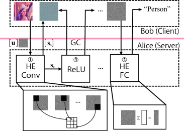
Figure 1: The general architecture of the Gazelle inference engine. The ${\mathsf{FC}}$ layer, much like the ${\mathsf{Conv}}$ layers, is internally a homomorphic matrix-vector product.

The main procedures of Gazelle [19] can be summarized using the example network architecture shown in Fig. 1. As shown in the figure, the protocol consists of three types of layers: ➀ the convolution layer ${\mathsf{Conv}}$, ➁ the fully-connected layer ${\mathsf{FC}}$, and ➂ the non-linear layers such as ReLU and image pooling. Assuming the input image $U$ is of dimension $n_{o}\times n_{i}$, Alice flattens $U$ as a vector ${\bf{u}}_{0}\in{\mathbb{Z}}_{p}^{n_{u}}$, where $n_{u}=n_{o}\cdot n_{i}$ (i.e., $U$ is raster scanned into ${\bf{u}}$). The protocol starts with Alice who encrypts ${\bf{u}}$ using some PAHE scheme and sends $[{\bf{u}}]$ to Bob. Upon receiving the ciphertext, Bob performs the corresponding computations depending on the layer type.
➀   For ${\mathsf{Conv}}$ layers, Bob homomorphically convolves $[{\bf{u}}]$ with a plaintext weight filter $W\in{\mathbb{Z}}^{f_{h}\times f_{w}}_{p}$. The convolved result, $[{\bf{y}}]=[W*{\bf{u}}]$, is randomized by a share of secret ${\bf{s}}_{B}$ as

$$\mathsf{HomShare}([{\bf{y}}])=([{\bf{s}}_{A}],{\bf{s}}_{B})=([{\bf{y}}-{\bf{s}}_{B}\bmod{p_{\rm A}}],{\bf{s}}_{B})$$ (2)

with some prime modulus $p_{\rm A}$. $[{\bf{s}}_{A}]$ is returned to Alice, and Bob keeps ${\bf{s}}_{B}$.
➁   For ${\mathsf{FC}}$ layers, Bob computes some matrix-vector product $[{\bf{y}}]=[W\cdot{\bf{u}}]$ for a plaintext weight matrix $W\in{\mathbb{Z}}^{n_{o}\times n_{i}}$, and randomizes the result similarly to the ${\mathsf{Conv}}$ layers.
➂   For non-linear layers, Gazelle evaluates the inputs in three steps:
1) obliviously compute ${\bf{y}}={\bf{s}}_{A}+{\bf{s}}_{B}$ to de-randomize ${\bf{y}}$ computed in linear layers using Bob’s input ${\bf{s}}_{B}$ with GC or multiplication triplets,
2) compute the non-linear function $f$ (e.g., ReLU or square from [21]) on ${\bf{y}}$, and
3) re-randomize the result $f({\bf{y}})$ using another share of secret, ${\bf{s}}_{B,1}$ from Bob, and output ${\bf{s}}_{A,1}=f({\bf{y}})-{\bf{s}}_{B,1}\bmod{p_{\rm A}}$ for Alice, and ${\bf{s}}_{B,1}$ for Bob.
Upon receiving the outputs from GC, Alice encrypts ${\bf{s}}_{A,1}$ as $[{\bf{s}}_{A,1}]$, and send the ciphertext to Bob. Bob then computes

$$[f({\bf{y}})]=\mathsf{HomRec}([{\bf{s}}_{A}],{\bf{s}}_{B})=[{\bf{s}}_{A}+{\bf{s}}_{B}\bmod{p_{\rm A}}]$$ (3)

using $[{\bf{s}}_{A,1}]$ and ${\bf{s}}_{B,1}$, and obtains $[f({\bf{y}})]$. Bob can then start a new round of linear evaluation (steps ➀ and ➁), until all layers are evaluated.

3.3 Homomorphic Convolution

One of the main computational bottlenecks in a typical CNN architecture [20, 15, 16] is the evaluations of the large number of ${\mathsf{Conv}}$ layers. While ${\mathsf{Conv}}$ only involves the simple calculation of a series of inner products, the homomorphic version of inner product is complex to compute. For example, in BFV, for some ciphertext vector $[{\bf{u}}]$ and plaintext vector ${\bf{w}}$, an inner product $[v]=[{\bf{w}}\cdot{\bf{u}}]$ is computed as

$$[{\bf{v}}] ={\bf{w}}\boxcircle[{\bf{u}}],\text{and }[y]=\sum_{i=1}^{\lg{(n)}}{\mathsf{rot}}\left([{\bf{v}}],\frac{n}{2^{i}}\right).$$ (4)

where expensive homomorphic rotations are required to accumulate the multiplication results. As it turns out, the ${\mathsf{rot}}$ operation is expensive in terms of both computational time and communicational bandwidth. Therefore, one of the main objectives of ENSEI is to eliminate this complex homomorphic rotate-and-accumulate process.

4 Oblivious Homomorphic Convolution in the Frequency Domain

If homomorphic convolution is expensive, a natural question to ask is that if we can avoid this operation in the first place. The convolution theorem tells us that for two discrete sequences ${\bf{w}}$ and ${\bf{u}}$, there exists a general transformation ${\mathsf{DFT}}$ in the form

$${\mathsf{DFT}}({\bf{x}})_{k}=\sum_{i=0}^{n_{f}-1}x_{i}\cdot\omega^{ik},$$ (5)

where the following property holds

$${\mathsf{DFT}}({\bf{w}}*{\bf{u}})={\mathsf{DFT}}({\bf{w}})\circ{\mathsf{DFT}}({\bf{u}}).$$ (6)

Without loss of generality, we assume that the length of the signals to be convolved is $n_{f}$, which is basically the filter dimension in secure inference (i.e., $n_{f}=f_{h}\cdot f_{w}$). Here, $\omega$ is the $n$-th root of unity in some field ${\mathbb{F}}$ (i.e., $\omega^{n}=1$ over ${\mathbb{F}}$). As shown in [1], if we choose finite fields as ${\mathbb{F}}$, we obtain the number theoretic transform (NTT), and Eq. (6) still holds. For unencrypted convolution (e.g., frequency-domain convolution algorithms adopted in CNN libraries), the NTT-based approach is not particularly attractive in terms of its performance, due to the additional reductions modulo some large field prime.

We observe a major difference in the encrypted domain. The main benefit for adopting NTT as the ${\mathsf{DFT}}$ operator in secure inference is that, in a cryptographic setting, finite fields are more natural to use than the complex number field. Most cryptographic primitives that build on established hardness assumptions live in finite fields, where arithmetic operations do not handle real numbers (and complex numbers) particularly well. Therefore, in this work, we use NTT as our main transformation realization.

4.1 ENSEI: The General Protocol

$$\boxed{\begin{array}[]{c c c c}&\text{Alice}&&\text{Bob}\\ 1.&{\hat{{\bf{u}}}}_{0}={\mathsf{DFT2D}}(U)&&\\ 2.&\left[{\hat{{\bf{u}}}}_{0}\right]=\operatorname{\mathsf{Enc}}({\hat{{\bf{u}}}}_{0},{\mathcal{K}})&&\\ 3.&&\xrightarrow{\hskip 6.99997pt\left[{\hat{{\bf{u}}}}_{0}\right]\hskip 6.99997pt}&\left[{\hat{{\bf{u}}}}_{0}\circ{\hat{{\bf{w}}}}_{0}\right]=\left[{\hat{{\bf{u}}}}_{0}\right]\boxcircle{\hat{{\bf{w}}}}_{0}\\ 4.&&&\left[{\hat{{\bf{s}}}}_{A,0}\right],{\hat{{\bf{s}}}}_{B,0}=\mathsf{HomShare}(\left[{\hat{{\bf{u}}}}_{0}\circ{\hat{{\bf{w}}}}_{0}\right])\\ 5.&{\hat{{\bf{s}}}}_{A,0}=\operatorname{\mathsf{Dec}}(\left[{\hat{{\bf{s}}}}_{A,0}\right])&\xleftarrow{\hskip 6.99997pt\left[{\hat{{\bf{s}}}}_{A,0}\right],\hskip 6.99997pt}&\\ 6.&{\bf{s}}_{A,0}={\mathsf{IDFT2D}}({\hat{{\bf{s}}}}_{A,0})&&{\bf{s}}_{B,0}={\mathsf{IDFT2D}}({\hat{{\bf{s}}}}_{B,0})\\ \\ 7.&\xrightarrow{\hskip 6.99997pt{\bf{s}}_{A,0}\hskip 6.99997pt}&\text{Activation}&\xleftarrow{\hskip 6.99997pt{\bf{s}}_{B,0}\hskip 6.99997pt}\\ 8.&\xleftarrow{\hskip 6.99997pt{\bf{s}}_{A,1}\hskip 6.99997pt}&\text{Function}&\xrightarrow{\hskip 6.99997pt{\bf{s}}_{B,1}\hskip 6.99997pt}\\ 9.&{\hat{{\bf{s}}}}_{A,1}={\mathsf{DFT2D}}({\bf{s}}_{A,1})&&{\hat{{\bf{s}}}}_{B,1}={\mathsf{DFT2D}}({\bf{s}}_{B,1})\\ 10.&\left[{\hat{{\bf{s}}}}_{A,1}\right]=\operatorname{\mathsf{Enc}}({\hat{{\bf{s}}}}_{A,1},{\mathcal{K}})&&\\ 11.&&\xrightarrow{\hskip 6.99997pt\left[{\hat{{\bf{s}}}}_{A,1}\right]\hskip 6.99997pt}&\left[{\hat{{\bf{u}}}}_{1}\right]=\mathsf{HomRec}(\left[{\hat{{\bf{s}}}}_{A,1}\right],{\hat{{\bf{s}}}}_{B,1})\\ 12.&&&\left[{\hat{{\bf{u}}}}_{1}\circ{\hat{{\bf{w}}}}_{1}\right]=\left[{\hat{{\bf{u}}}}_{1}\right]\boxcircle{\hat{{\bf{w}}}}_{1}\\ 13.&&&\left[{\hat{{\bf{s}}}}_{A,2}\right],{\hat{{\bf{s}}}}_{B,2}=\mathsf{HomShare}(\left[{\hat{{\bf{u}}}}_{1}\circ{\hat{{\bf{w}}}}_{1}\right])\\ 14.&{\hat{{\bf{s}}}}_{A,2}=\operatorname{\mathsf{Dec}}(\left[{\hat{{\bf{s}}}}_{A,2}\right])&\xleftarrow{\hskip 6.99997pt\left[{\hat{{\bf{s}}}}_{A,2}\right]\hskip 6.99997pt}&\\ &&\vdots&\end{array}}$$

Figure 2: The start and intermediate rounds of the Gazelle protocol with frequency-domain convolution via ${\mathsf{DFT}}$.

Before delving into the actual protocol, we provide a brief summary of the notations used in this section to improve the readability of the derivations.

• ${\bf{u}}$, ${\bf{w}}$: vectors denoting the plaintext input image and weights, respectively. When vectors are transformed into the frequency domain, we add a hat, e.g., ${\hat{{\bf{u}}}}$.

• ${\bf{s}}_{A,0}$, ${\bf{s}}_{B,0}$: vectors referring to the secret shared vectors for Alice and Bob, respectively, in the zeroth round of communication.

• $n_{o},n_{i},f_{h},f_{w}$: the image and filter dimensions.

• $n,p_{\rm E},q$: the RLWE parameters shown in Section 3.1.

• $p_{\rm N},p_{\rm A}$: the NTT and the secret sharing moduli, respectively.

Figure 2 details the general protocol for an oblivious homomorphic convolution in the frequency domain. In this protocol, we assume the existence of a pair of general discrete Fourier transform (DFT) operators ${\mathsf{DFT}}$ and ${\mathsf{IDFT}}$, and a pair of homomorphic secret sharing (HSS) scheme $\mathsf{HomShare}$ and $\mathsf{HomRec}$ (as depicted in Eq. (2) and (3)) for randomization and derandomization. In what follows, we provide a detailed explanation on the proposed protocol.

First, we say that Alice holds some two-dimensional plaintext input image $U\in{\mathbb{Z}}^{n_{o}\times n_{i}}$. Alice wants to inference on $U$ with a set of filters $\{W\in{\mathbb{Z}}^{f_{h}\times f_{w}}\}$ held by Bob. The protocol is executed as follows.

1. Line 1–3, Alice: Alice first pads the input according to the convolution type (e.g., same or valid), and computes a two-dimensional DFT on $U$ as ${\mathsf{DFT2D}}(U)$. Here, ${\mathsf{DFT2D}}$ is the two-dimensional DFT operator. Alice flattens the frequency-domain matrix to ${\hat{{\bf{u}}}}$ and encrypts it using $\operatorname{\mathsf{Enc}}$. The encrypted ciphertext $[{\hat{{\bf{u}}}}]=\operatorname{\mathsf{Enc}}({\hat{{\bf{u}}}})$ is transferred to Bob through public channels.

2. Line 3–4, Bob: Bob also performs similar padding, DFT, and the flatten operations on the (unencrypted) weight matrix, obtaining ${\hat{{\bf{w}}}}={\mathsf{flatten}}({\mathsf{DFT2D}}(W))$ as the result. Upon receiving $[{\hat{{\bf{u}}}}]$, Bob carries out the frequency-domain homomorphic convolution by computing a simple homomorphic Hadamard product between $[{\hat{{\bf{u}}}}]$ and transformed plaintext ${\hat{{\bf{w}}}}$. In order to prevent weight leakages, Bob applies $\mathsf{HomShare}$ from the HSS protocol and acquires two shares of secrets $[{\hat{{\bf{s}}}}_{A,0}]$ and ${\hat{{\bf{s}}}}_{B,0}$ according to Eq. (2). Bob sends the shared secret $[{\hat{{\bf{s}}}}_{A,0}]$ back to Alice.

3. Line 4–6, Alice: Alice decrypts $[{\hat{{\bf{s}}}}_{A,0}]$ as ${\hat{{\bf{s}}}}_{A,0}$. Both Alice and Bob apply ${\mathsf{IDFT}}$ to the shares of secret to obtain

   $${\bf{s}}_{A,0} ={\mathsf{IDFT}}({\hat{{\bf{s}}}}_{A,0})$$

   $$={\mathsf{IDFT}}({\hat{{\bf{u}}}}_{0}\circ{\hat{{\bf{w}}}}_{0}-{\hat{{\bf{s}}}}_{B,0})\bmod{p_{\rm A}}$$ (7)

   $${\bf{s}}_{B,0} ={\mathsf{IDFT}}({\hat{{\bf{s}}}}_{B,0})\bmod{p_{\rm A}},$$ (8)

   marking the end of the evaluation for the first convolution layer in the NN. We note that when the ${\mathsf{IDFT}}$ operator is error free, Eq. (7) evaluates to

   $${\mathsf{IDFT}}({\hat{{\bf{u}}}}_{0}\circ{\hat{{\bf{w}}}}_{0}-{\hat{{\bf{s}}}}_{B,0})\bmod{p_{\rm A}}$$

   $$={\mathsf{IDFT}}({\hat{{\bf{u}}}}_{0}\circ{\hat{{\bf{w}}}}_{0})-{\mathsf{IDFT}}({\hat{{\bf{s}}}}_{B,0})\bmod{p_{\rm A}}$$ (9)

   $$={\bf{u}}_{0}*{\bf{w}}_{0}-{\bf{s}}_{B,0}\bmod{p_{\rm A}}.$$ (10)

4. Line 7–8, Alice and Bob: In implementing oblivoius activation, the essential computations involved in GC (or multiplication triples) can be formulated as

   $${\bf{u}}_{0}*{\bf{w}}_{0} ={\bf{s}}_{A,0}+{\bf{s}}_{B,0}\bmod{p_{\rm A}}$$ (11)

   $${\bf{u}}_{1} =f({\bf{u}}_{0}*{\bf{w}}_{0})$$ (12)

   $${\bf{s}}_{A,1} ={\bf{u}}_{1}-{\bf{s}}_{B,1}\bmod{p_{\rm A}},$$ (13)

   where $f$ is some activation function (e.g., ReLU). As mentioned, the above procedure only remains correct if the underlying ${\mathsf{DFT}}$ operator satisfies Eq. (9).

5. Line 9–10, Alice: Upon receiving the computed results from oblivious activation, Alice repeats the process of Line 1–3. The transformed and encrypted inputs $[{\hat{{\bf{s}}}}_{A,1}]$ are again sent to Bob.

6. Line 11–13, Bob: The final step to complete the proposed protocol is the $\mathsf{HomRec}$ procedure as in Eq. (3). Since $[{\hat{{\bf{s}}}}_{A,1}]=[{\mathsf{DFT}}({\bf{u}}_{1}-{\bf{s}}_{B,1})]$ and ${\hat{{\bf{s}}}}_{B,1}={\mathsf{DFT}}({\bf{s}}_{B,1})$, when the same condition in Eq. (9) holds, we have

   $$[{\mathsf{DFT}}({\bf{u}}_{1}-{\bf{s}}_{B,1})]\boxplus{\mathsf{DFT}}({\bf{s}}_{B,1})$$ (14)

   $$=[{\hat{{\bf{u}}}}_{1}-{\mathsf{DFT}}({\bf{s}}_{B,1})+{\mathsf{DFT}}({\bf{s}}_{B,1})]=[{\hat{{\bf{u}}}}_{1}]$$ (15)

   and a new round of FDSC can be carried out.

The evaluation of any CNN can be decomposed into the repetitions of the above procedures, as our protocol is essentially a way of obliviously moving into and out of the frequency domain.

Note that the DFT operator in Fig. 2 does not have to be NTT. However, adopting NTT in the protocol requires minimal modification, as we only need to replace the ${\mathsf{DFT}}$ and ${\mathsf{IDFT}}$ operators in Fig. 2 with ${\mathsf{NTT}}$ and ${\mathsf{INTT}}$. In this case, in addition to the secret sharing modulus $p_{\rm A}$ and encryption modulus $p_{\rm E}$, we need a third modulus $p_{\rm N}$ for ENSEI-NTT. In other words, we have $\omega^{n}\equiv 1\bmod{p_{\rm N}}$, and the corresponding transformation is written as

$${\mathsf{NTT}}({\bf{x}})_{k}=\sum_{i=0}^{n_{f}-1}x_{i}\omega^{ik}\bmod{p_{\rm N}}.$$ (16)

4.1.1 Correctness for NTT-based ENSEI

Here, the correctness of the NTT version of our protocol is briefly explained, and a more detailed discussion can be found in the appendix. We assert that due to the need of finite-field arithmetic, not every pair of ${\mathsf{DFT}}$ operators work for the above protocol. The most important condition to ensure correctness is that Eq. (9) equals to Eq. (10), and that Eq. (14) equals to Eq. (15). If we instantiate ENSEI with NTT, then, the correctness holds when the following statement is true

$${\mathsf{INTT}}({\hat{{\bf{u}}}}\circ{\hat{{\bf{w}}}}-{\hat{{\bf{s}}}}_{B})\bmod{p_{\rm A}}$$ (17)

$$=({\mathsf{INTT}}({\hat{{\bf{u}}}}\circ{\hat{{\bf{w}}}})-{\mathsf{INTT}}({\hat{{\bf{s}}}}_{B}))\bmod{p_{\rm A}}$$ (18)

$$=({\bf{u}}*{\bf{w}}-{\bf{s}}_{B})\bmod{p_{\rm A}}.$$ (19)

The convolution result ${\bf{u}}*{\bf{w}}$ can be recovered by applying the recovery procedure of HSS, under the condition that the HSS modulus $p_{\rm A}$ is larger than the NTT modulus $p_{\rm N}$. A similar procedure also ensures the correctness of Eq. (14) and Eq. (15).

4.1.2 Security

In terms of security properties, our protocol is basically identical to the linear kernel in Gazelle [19], so a formal proof is left out. Briefly speaking, given the security of the PAHE scheme, Bob cannot temper the encrypted inputs of Alice (e.g., ${\bf{u}}$), and with HSS, Alice gains no knowledge of the models from Bob (e.g., ${\bf{w}}$).

5 Integration and Parameter Instantiation

5.1 Reducing the Number of DFT in ENSEI

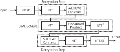
Figure 3: The overview for a sequence of $\operatorname{\mathsf{Enc}}$-${\mathsf{SIMDScMult}}$-$\operatorname{\mathsf{Dec}}$ procedures based on ENSEI for general AHE schemes.

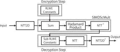
Figure 4: Modified $\operatorname{\mathsf{Enc}}$-${\mathsf{SIMDScMult}}$-$\operatorname{\mathsf{Dec}}$ for Gazelle-like networks to reduce the extra NTTs for plaintext packing.

The plaintext packing technique [28] used for embedding a vector of plaintext integers ${\bf{u}}\in{\mathbb{Z}}^{n}_{p}$ into a single ciphertext pair relies on the idea that a large-degree polynomials (with proper modulus) can be decomposed into a set of independent polynomials that are of smaller degrees. The exact procedures for lattice-based PAHE is sketched in Fig. 3, where we can see that during encryption, a vector of plaintext is transformed into the time domain via the ${\mathsf{INTT}}$ operation and embedded into the ciphertext. Later in the evaluation stage, ${\mathsf{SIMDScMult}}$ re-applies ${\mathsf{NTT}}$ on the ciphertext (and thus simultaneously on the plaintext) followed by an element-wise multiplication, which also conducts the coefficient-wise multiplication on the plaintext vector. We see that while Fig. 3 is a straightforward application of ENSEI, it clearly involves redundant NTTs.

Our key observation here is that, the internal operation of a ${\mathsf{SIMDScMult}}$ is merely conducting frequency-domain multiplication of polynomials (shown in Fig. 3), as it is known that a multiplication between two polynomials in some particular quotient rings equates to a (nega-)cyclic convolution of their coefficients. Therefore, we can directly embed the NTT2D-transformed frequency-domain image into the NTT transformed ciphertext (i.e., $\hat{a}\cdot\hat{s}+{\mathsf{NTT2D}}(U)$), as depicted in Fig. 4, and execute ${\mathsf{SIMDScMult}}$ without NTT operations during the encryption stage (the RLWE constants can be generated offline). By performing the entire $\operatorname{\mathsf{Enc}}$-${\mathsf{SIMDScMult}}$ process in the frequency domain, we can reduce two NTT butterflies per convolution. Note that, because the homomorphic rotations employed in Gazelle (${\mathsf{rot}}$) force several rounds of NTTs for switching the decryption keys (such that proper keys are generated to decrypt the rotated ciphertext), ENSEI needs much less NTT runs compared to the time-domain convolution devised by Gazelle. The only restriction in ENSEI is that the plaintext modulus $p_{\rm E}$ needs to be larger than the ENSEI modulus $p_{\rm N}$. Further elaborations on the exact precision settings that satisfy the requirement $p_{\rm E}\geq p_{\rm N}$ is discussed in the experiment.

5.2 The Moduli and RLWE Parameters

In ENSEI, we have three moduli to consider: the secret sharing modulus $p_{\rm A}$, the encryption modulus $p_{\rm E}$, and the NTT modulus $p_{\rm N}$. The three moduli need to satisfy the relation $p_{\rm E}\geq p_{\rm A}\geq p_{\rm N}$. As it turns out, $p_{\rm N}$ is determined by two factors: i) the maximum value in the matrix operands, and ii) the length of the convolving sequence. For two sequences ${\bf{u}}\in{\mathbb{Z}}^{n_{o}\times n_{i}}$ and ${\bf{w}}\in{\mathbb{Z}}^{f_{h}\cdot f_{w}}$, the lower bound on $p_{\rm N}$ can be written as

$$p_{\rm N}\geq\max({\bf{u}})\cdot\max({\bf{w}})\cdot f_{h}\cdot f_{w}.$$ (20)

Suppose $n_{f}=f_{h}\cdot f_{w}$, in a typical CNN setting, compared to the RLWE lattice dimension $n$, $n_{f}$ is generally small (e.g., $n_{f}=9$ for the $3\times 3$ filters used in the experiment). In addition, in hardware-friendly network architectures, such as BinaryConnect [8] or BinaryNet [9], $\max({\bf{u}})$ is generally less than 10-bit, and $\max({\bf{w}})$ is even smaller.

As described, $p_{\rm E}$ only needs to be as large as $p_{\rm N}$. This is not a problem when $p_{\rm N}$ is large. However, when all the terms in Eq. (20) is small, we can set $p_{\rm N}$ to be extremely small, but not $p_{\rm E}$. For security reasons, $n$ needs to be a relative large power of 2 (e.g., 1024 to 2048), and $p_{\rm E}$ can only be as small as the smallest prime that completely splits over the field $x^{n}+1$ (e.g., for $n=2048$, $p_{\rm E}\geq 12289$), and we cannot set $p_{\rm E}=p_{\rm N}$ if $p_{\rm N}<12289$. Fortunately in this case, since $p_{\rm N}$ is not related to the security of PAHE, we can still use a smaller $p_{\rm N}$ to transform the weight matrix. The small size of $p_{\rm N}$ makes the coefficients of the transformed weight matrix small, thereby reducing the noise growth and the size of the ciphertext modulus.

6 Complexity Analysis and Numerical Experiments

6.1 Complexity Analysis for ENSEI

Given the integrated protocol, we give a comparison between the asymptotic computational complexity of Gazelle and ENSEI. We formulate the complexity based on three basic operations, $t_{p_{\rm E}}$, $t_{q}$, and $t_{p_{\rm N}}$, which are the respective time of performing a multiplication modulo $p_{\rm E}$, $q$, and $p_{\rm N}$. As described above, we assume the convolution is performed between the input $U$ of dimension $n_{u}=n_{o}\times n_{i}$, and $W$ of dimension $n_{f}=f_{h}\times f_{w}$. We also use $\beta_{n_{u}}$ for $\lceil\frac{n_{u}}{n}\rceil$, the ratio between the input image dimension and lattice dimension. For ENSEI-NTT, we have

$$\beta_{n_{u}}\big{(}4\cdot(n\cdot\log(n_{u})\cdot t_{p_{\rm N}})+n\cdot t_{q}+2\cdot n\log(n)\cdot t_{q}\big{)},$$ (21)

which is of order $\mathcal{O}(n_{u}\cdot\log(n_{u}))$, since the RLWE parameter $n$ is a constant. In Eq. (21), the forward NTTs on $U$ and $W$, and the backward inverse NTT on the convolution result and randomization vector counts for four transformations over the field ${\mathbb{F}}_{p_{\rm N}}$. The last term in Eq. (21) counts for the encryption and decryption costs, where NTTs are performed on the ciphertext with lattice dimension $n$. Since Gazelle [19] did not provide formal complexity calculations, the analyses here are only of estimations.

$$\beta_{n_{u}}\big{(}2\cdot n\log(n)\cdot t_{q}+(n_{i}\cdot f_{w}-1)\cdot(n_{o}\cdot f_{h}-1)\cdot n\cdot t_{q}+$$

$$n\log(n)\cdot t_{q}+n\log(n)\cdot t_{Q}\big{)},$$ (22)

where $t_{Q}$ is the time for generating the Galois key with a slightly larger modulus $Q$, as described in [14]. Two points are emphasized here. First, it can be seen that the second term in Eq. (6.1) depends on both the input image and filter window, which means that the complexity is of $\mathcal{O}(n_{u}\cdot\log(n_{u})\cdot n_{f})$. In contrast, ENSEI-NTT is only of $\mathcal{O}(n_{u}\cdot\log(n_{u}))$. This is the primary reason why Gazelle does not scale well, as both the time for rotation and the ciphertext modulus $q=\mathcal{O}(\mathsf{Poly}(p_{\rm E}))$ increase as a result of larger weight matrices.

Table 1: Prediction Accuracy on the CIFAR-10 Dataset

Precision	Input	Filter	Accuracy
	Bit Width	Bit Width
Binary	8	1	81%
Medium	8	4	79%
High	11	7	82%
High-Square	11	7	82%
Full	32	32	83%
[21, 19]	-	-	82%

Table 2: Proposed Candidate Parameter Sets

Protocol	Parameter	Binary	Medium	High
ENSEI-NTT	$p_{\rm N}$	2311	147457	2359303
	$\lceil\lg{p_{\rm N}}\rceil$	11	12	18
	$p_{\rm E}$	12289	147457	2363393
	$\lceil\lg{p_{\rm E}}\rceil$	14	18	22
	$\lceil\lg{q}\rceil$	45	53	60
	$n$	2048	2048	2048

Table 3: Computational Cost of ENSEI with Respect to Different Parameter Sets Measured in Microseconds

	Precision	Image	Encryption	Filtering	Result	$t_{\rm online}$	PAHE	Filter	$t_{\rm setup}$	Galois-Key
		Read	Constants	(Hadamard)	Decryption		Setup	Read		Generation
ENSEI-NTT	Binary	197.4	92.1	146.7 (7.3)	150.6	587.1	21972.2	1l0.6	22082.8	76983.2
ENSEI-NTT	High	197.3	92.4	147.5 (7.3)	151.2	588.5	21351.6	110.2	21462.2	77039.3

Table 4: Convolution Benchmarks w.r.t Precision Levels

	Input Dim.	Filter Dim.	Precision	$t_{\rm setup}$	$t_{\rm online}$	Bandwidth
Gazelle	$(28\times 28\times 1)$	$(5\times 5\times 5)$	-	11.4 ms	9.20 ms	130 KB
Gazelle	$(32\times 32\times 32)$	$(3\times 3\times 32)$	-	704 ms	195 ms	-
ENSEI-NTT	$(28\times 28\times 1)$	$(5\times 5\times 5)$	Binary	22.0 ms	1.8 ms	23.0 KB
ENSEI-NTT	$(28\times 28\times 1)$	$(5\times 5\times 5)$	High	21.4 ms	1.8 ms	30.1 KB
ENSEI-NTT	$(32\times 32\times 32)$	$(3\times 3\times 32)$	Binary	22.0 ms	16.9 ms	368 KB
ENSEI-NTT	$(32\times 32\times 32)$	$(3\times 3\times 32)$	High	21.4 ms	16.9 ms	492 KB

6.2 Experiment Setup

In order to quantitatively assess the impact of ENSEI on secure inference, we implemented the ENSEI protocol using the SEAL library [6] in C++. We also performed accuracy test to estimate the smallest NTT modulus $p_{\rm N}$ for different parametrizations of PAHE.

Most existing works [19, 21] only show the main accuracy and performance results on either MNIST or CIFAR-10, or even smaller datasets [25]. For fair comparisons, we first report accuracy and quantization experiments using the same architecture in one of the most recent works [19], and then compare ENSEI-based SI on other architectures (with different protocols) suggested in [25]. The accuracy results are obtained using the Tensorflow library [13], and the runtime of homomorphic convolution is recorded on an Intel Core i3-7100 CPU 3.90 GHz processor.

6.3 CNN Prediction Accuracy

Using the same architecture in [19, 21], Table 1 illustrates how the prediction accuracy improves as the bit precision increases in SI. We observe that for 11-bit features and 7-bit weights, the accuracy is on an equivalent level to the full-bit precision case (the difference is less than 1%). Meanwhile, the binary-weight instance can reach a final prediction accuracy of 81%, which is only 1% less than the original accuracy reported in [19, 21] (we may have used different hyperparameters).

As later observed in Section 6.6, using GC-based ReLU on the first several convolution layers brings significant performance overhead to both existing works [19, 21] and ENSEI. Therefore, we experimented on a different network architecture, where some of the ReLU layers are replaced with the square activation (SA) function proposed in [21]. We found that replacing a small amount of ReLU with SA (denoted as High-Square in Table 1) does not affect the prediction accuracy much, while replacing all ReLU layers with SA does (accuracy becomes only 10%). Nonetheless, even replacing a small portion of ReLU with SA proves to be critical in improving the practicality of ENSEI-based SI, as demonstrated in Section 6.6.

6.4 Quantization and Parameter Instantiations

From the previous section, we obtain the maximum values on ${\bf{u}}$ and ${\bf{w}}$. Hence, we can apply Eq. (20) to instantiate three sets of RLWE parameters for adopting the fine-grained layer-to-layer (and network-to-network) precision adjustment. We take the high-precision case with a $3\times 3$ filter size as an example. For 12-bit ${\bf{u}}$ and 6-bit ${\bf{w}}$, $p_{\rm N}$ needs to satisfy

$$p_{\rm N}\geq 2^{12}\cdot 2^{6}\cdot 9,$$ (23)

and that $p_{\rm N}\equiv 1\bmod{3}$. The lattice dimension $n$ is fixed to be 2048 to ensure efficient packing and a 128-bit security. We find the minimal $p_{\rm E}\geq p_{\rm N}$ for the $p_{\rm N}$ required such that $p_{\rm E}\equiv 1\bmod{n}$. Finally, the ciphertext modulus $q$ is adjusted accordingly to tolerate the error growth while retaining the security requirement, with overwhelming decryption success probability (the discrete Gaussian parameter $\sigma$ is set to 4).

The calculated moduli and instantiated parameters are shown in Table 2. Using a $p_{\rm N}$ that is much smaller than $p_{\rm E}$, we generate less noises in the ciphertext, and the Binary parameter set enjoys from a smaller ciphertext modulus. The resulting ciphertext is 33% smaller than the High parameter set, as shown in Section 6.5.

6.5 Efficiency Comparison to Gazelle

We summarize the performance data of ENSEI-NTT with respect to different parameter instantiations in Table 3. The running times are an average of 10,000 trials measured in microseconds. Here, $t_{\rm setup}$ is time consumed by procedures that do not involve user inputs. Likewise, $t_{\rm online}$ refers to the time for input-dependent steps, and is the sum of all terms in Table 3 up to $t_{\rm online}$ horizontally. In particular, the results show that the time it takes to compute the Hadamard product (shown in parenthesis after the Filter column) is only a fraction of the time consumed by the NTT operations (the filtering step contains two NTT butterflies), which need to be applied once per each of the input and filter channels.

Using the instantiated parameters and recorded speed, the performance comparison of ENSEI-NTT and Gazelle on a set of convolution benchmarks are summarized in Table 4. In Table 4, we see that for larger benchmarks, the online convolution time is reduced by nearly 11x across all precisions with ENSEI-NTT. In addition, we point out that the setup time of ENSEI scales extremely slowly with the dimensions of the images and filters. Therefore, we observe a nearly 34x reduction in setup time for the larger benchmarks. In combined, ENSEI-NTT obtains a 23x reduction in total time for a 32-channel convolution.

6.6 Architectural Comparisons

Table 5: The Impact of Neural Architecture on Inference Time

Architecture	#Conv	Accuracy	ENSEI	Prior Arts
			Total Time	Time
Fig. 13 in [21]	7	82%	7.72 s	12.9 s
High-Square	7	82%	1.38 s	-
BC2 in [25]	9	82%	2.76 s	4.8 s
BC3 in [25]	9	86%	14.7 s	35.8 s
BC4 in [25]	11	88%	30.91 s	123.9 s
BC5 in [25]	17	88%	30.98 s	147.7 s

Lastly, we compare different architectures with and without FDSC to demonstrate the effectiveness of the ENSEI protocol. Table 5 summarizes the inference time with respect to increasingly deep neural architectures, and the accuracy is measured on the CIFAR-10 dataset. We first observe that, while HE-based linear layers represent a large portion of the computational time (from 40% up to 80% of the total inference time), the GC-based non-linear ReLU computations become the bottleneck when ENSEI is employed. By replacing the second and fifth ReLU layer in the benchmark architecture (the complete architecture can be found in the appendix), the online SI time can be reduced to 1.38 seconds, nearly 10x faster than the baseline method. Using ENSEI, what we discovered is that, under the same accuracy constraint, certain neural architectures are much more efficient when implemented using secure protocols. Hence, efficient ways of finding such architecture becomes an important future area of research.

7 Conclusion

In this work, we proposed ENSEI, a frequency-domain convolution technique that accelerates CNN-based secure inference. By using a generic DFT, we show that oblivious convolution can be built on any encryption scheme that is additively homomorphic. In particular, we instantiate and integrate ENSEI with NTT and compare ENSEI-NTT to one of the most recent work on secure inference, Gazelle. In the experiment, we observed up to 23x reduction in convolution time, and up to 10x in the overall inference time. We demonstrate that PAHE-based protocol is one of the simplest and most practical secure inference scheme.

References

- [1] Ramesh C Agarwal and C Sidney Burrus. Number theoretic transforms to implement fast digital convolution. Proceedings of the IEEE, 63(4):550–560, 1975.
- [2] Zvika Brakerski. Fully homomorphic encryption without modulus switching from classical GapSVP. In Advances in Cryptology–CRYPTO 2012, pages 868–886. Springer, 2012.
- [3] Zvika Brakerski, Craig Gentry, and Vinod Vaikuntanathan. (Leveled) fully homomorphic encryption without bootstrapping. ACM Transactions on Computation Theory (TOCT), 6(3):13, 2014.
- [4] Alon Brutzkus, Oren Elisha, and Ran Gilad-Bachrach. Low latency privacy preserving inference. arXiv preprint arXiv:1812.10659, 2018.
- [5] Ankur Chattopadhyay and Terrance E Boult. Privacycam: a privacy preserving camera using uclinux on the blackfin dsp. In 2007 IEEE Conference on Computer Vision and Pattern Recognition, pages 1–8. IEEE, 2007.
- [6] Hao Chen, Kim Laine, and Rachel Player. Simple encrypted arithmetic library-seal v2. 1. In International Conference on Financial Cryptography and Data Security, pages 3–18. Springer, 2017.
- [7] Edward Chou, Josh Beal, Daniel Levy, Serena Yeung, Albert Haque, and Li Fei-Fei. Faster cryptonets: Leveraging sparsity for real-world encrypted inference. arXiv preprint arXiv:1811.09953, 2018.
- [8] Matthieu Courbariaux, Yoshua Bengio, and Jean-Pierre David. Binaryconnect: Training deep neural networks with binary weights during propagations. In Advances in neural information processing systems, pages 3123–3131, 2015.
- [9] Matthieu Courbariaux, Itay Hubara, Daniel Soudry, Ran El-Yaniv, and Yoshua Bengio. Binarized neural networks: Training deep neural networks with weights and activations constrained to+ 1 or-1. arXiv preprint arXiv:1602.02830, 2016.
- [10] Junfeng Fan and Frederik Vercauteren. Somewhat practical fully homomorphic encryption. IACR Cryptology ePrint Archive, 2012:144, 2012.
- [11] Ran Gilad-Bachrach, Nathan Dowlin, Kim Laine, Kristin Lauter, Michael Naehrig, and John Wernsing. Cryptonets: Applying neural networks to encrypted data with high throughput and accuracy. In International Conference on Machine Learning, pages 201–210, 2016.
- [12] Mahadevan Gomathisankaran, Xiaohui Yuan, and Patrick Kamongi. Ensure privacy and security in the process of medical image analysis. In 2013 IEEE International Conference on Granular Computing (GrC), pages 120–125. IEEE, 2013.
- [13] Google Inc. TensorFlow: Large-scale machine learning on heterogeneous systems, 2015. Software available from tensorflow.org.
- [14] Shai Halevi and Victor Shoup. Faster homomorphic linear transformations in helib. Technical report, Cryptology ePrint Archive, Report 2018/244, 2018.
- [15] Kaiming He, Xiangyu Zhang, Shaoqing Ren, and Jian Sun. Deep residual learning for image recognition. In Proceedings of the IEEE conference on computer vision and pattern recognition, pages 770–778, 2016.
- [16] Gao Huang, Zhuang Liu, Laurens Van Der Maaten, and Kilian Q Weinberger. Densely connected convolutional networks. In Proceedings of the IEEE conference on computer vision and pattern recognition, pages 4700–4708, 2017.
- [17] Xiaoqian Jiang, Miran Kim, Kristin Lauter, and Yongsoo Song. Secure outsourced matrix computation and application to neural networks. In Proceedings of the 2018 ACM SIGSAC Conference on Computer and Communications Security, pages 1209–1222. ACM, 2018.
- [18] Mika Juuti, Sebastian Szyller, Samuel Marchal, and N Asokan. Prada: protecting against dnn model stealing attacks. In 2019 IEEE European Symposium on Security and Privacy (EuroS&P), pages 512–527. IEEE, 2019.
- [19] Chiraag Juvekar, Vinod Vaikuntanathan, and Anantha Chandrakasan. Gazelle: A low latency framework for secure neural network inference. arXiv preprint arXiv:1801.05507, 2018.
- [20] Alex Krizhevsky, Ilya Sutskever, and Geoffrey E Hinton. Imagenet classification with deep convolutional neural networks. In Advances in neural information processing systems, pages 1097–1105, 2012.
- [21] Jian Liu, Mika Juuti, Yao Lu, and N Asokan. Oblivious neural network predictions via MinioNN transformations. In Proceedings of the 2017 ACM SIGSAC Conference on Computer and Communications Security, pages 619–631. ACM, 2017.
- [22] Eleftheria Makri, Dragos Rotaru, Nigel P. Smart, and Frederik Vercauteren. Epic: Efficient private image classification (or: Learning from the masters). Cryptology ePrint Archive, Report 2017/1190, 2017. https://eprint.iacr.org/2017/1190.
- [23] Payman Mohassel and Yupeng Zhang. Secureml: A system for scalable privacy-preserving machine learning. In 2017 38th IEEE Symposium on Security and Privacy (SP), pages 19–38. IEEE, 2017.
- [24] Yuriy Polyakov, Kurt Rohloff, and Gerard W. Ryan. Alisade lattice cryptography library. https://git.njit.edu/palisade/PALISADE, 2018.
- [25] M Sadegh Riazi, Mohammad Samragh, Hao Chen, Kim Laine, Kristin E Lauter, and Farinaz Koushanfar. Xonn: Xnor-based oblivious deep neural network inference. IACR Cryptology ePrint Archive, 2019:171, 2019.
- [26] Bita Darvish Rouhani, M Sadegh Riazi, and Farinaz Koushanfar. Deepsecure: Scalable provably-secure deep learning. In 2018 55th ACM/ESDA/IEEE Design Automation Conference (DAC), pages 1–6. IEEE, 2018.
- [27] Reza Shokri, Marco Stronati, Congzheng Song, and Vitaly Shmatikov. Membership inference attacks against machine learning models. In 2017 IEEE Symposium on Security and Privacy (SP), pages 3–18. IEEE, 2017.
- [28] Nigel P Smart and Frederik Vercauteren. Fully homomorphic encryption with relatively small key and ciphertext sizes. In International Workshop on Public Key Cryptography, pages 420–443. Springer, 2010.
- [29] Pablo Speciale, Johannes L Schonberger, Sing Bing Kang, Sudipta N Sinha, and Marc Pollefeys. Privacy preserving image-based localization. In Proceedings of the IEEE Conference on Computer Vision and Pattern Recognition, pages 5493–5503, 2019.
- [30] Binghui Wang and Neil Zhenqiang Gong. Stealing hyperparameters in machine learning. In 2018 IEEE Symposium on Security and Privacy (SP), pages 36–52. IEEE, 2018.
- [31] Zhenyu Wu, Zhangyang Wang, Zhaowen Wang, and Hailin Jin. Towards privacy-preserving visual recognition via adversarial training: A pilot study. In Proceedings of the European Conference on Computer Vision (ECCV), pages 606–624, 2018.
- [32] Andrew C Yao. Protocols for secure computations. In Foundations of Computer Science, 1982. SFCS’08. 23rd Annual Symposium on, pages 160–164. IEEE, 1982.