Geostatistical Modeling and Prediction
Using Mixed-Precision Tile Cholesky Factorization

Abstract

Geostatistics represents one of the most challenging classes of scientific applications due to the desire to incorporate an ever increasing number of geospatial locations to accurately model and predict environmental phenomena. For example, the evaluation of the Gaussian log-likelihood function, which constitutes the main computational phase, involves solving systems of linear equations with a large dense symmetric and positive definite covariance matrix. Cholesky, the standard algorithm, requires $O(n^{3})$ floating point operators and has an $O(n^{2})$ memory footprint, where n is the number of geographical locations. Here, we present a mixed-precision tile algorithm to accelerate the Cholesky factorization during the log-likelihood function evaluation. Under an appropriate ordering, it operates with double-precision arithmetic on tiles around the diagonal, while reducing to single-precision arithmetic for tiles sufficiently far off. This translates into an improvement of the performance without any deterioration of the numerical accuracy of the application. We rely on the StarPU dynamic runtime system to schedule the tasks and to overlap them with data movement. To assess the performance and the accuracy of the proposed mixed-precision algorithm, we use synthetic and real datasets on various shared and distributed-memory systems possibly equipped with hardware accelerators. We compare our mixed-precision Cholesky factorization against the double-precision reference implementation as well as an independent block approximation method. We obtain an average of 1.6X performance speedup on massively parallel architectures, while maintaining the accuracy necessary for modeling and prediction.

I Introduction

The rise of mixed-precision algorithmic developments in the scientific community coincides with the advent of machine learning techniques for performing analytics on big data problems. Because the convergence between HPC and big data [1] is now at the forefront of research innovations for the digital world, e.g., healthcare, security, and climate/weather modeling, hardware vendors have tremendously invested in designing chips during the last decade with an emphasis on further provisioning low precision floating-point units [2, 3]. This computing paradigm shift has mobilized researchers in identifying opportunities within their legacy numerical algorithms to exploit such hardware features. The main idea consists in determining which computational phases within an algorithm are resilient to a lower precision, while ultimately maintaining the required level of accuracy for the final solution. The availability of off-the-shelves hardware with effective support of low precision floating-point arithmetics has further democratized mixed-precision algorithms. This hardware/algorithm synergism has demonstrated to be a game-changing approach for solving some of the most challenging scientific problems [4].

Given this fertile landscape, we propose to study geostatistics modeling and prediction using mixed-precision algorithms. Rather than using first principles physics approaches, geostatistics may represent a plausible alternative to accurately model and predict environmental phenomena given the availability of measurements at a high number of geospatial locations. One of the main computational phases necessitates the evaluation of the Gaussian log-likelihood function, which translates into iteratively solving a number of large systems of linear equations. The large dense symmetric and positive definite covariance matrix can be processed with the Cholesky factorization with a cubic algorithmic complexity as the number of geographical locations with measurements grow. There are several methodologies to reduce this intractable complexity, e.g., dimension-reducing PCA approaches, independent block approximation method [5], or low-rank approximations [6], to name a few. These methods are thoroughly described and evaluated in [7].

In this paper, we present a new mixed-precision algorithm to accelerate the Cholesky factorization during the log-likelihood function evaluation in the context of environmental applications. Based on tile algorithms [8], the resulting Cholesky factorization takes advantage of the covariance matrix structure, which retains the most significant information around the diagonal of the matrix. Instead of completely annihilating the off-diagonal contributions engendering a possible loss of accuracy, we operate the computation of close-to-diagonal tiles in double-precision accuracy while switching to single-precision accuracy for the remaining far off-diagonal tiles. Insight into the application data sparsity is paramount to take into account, before moving forward with mixed-precision algorithms. While mixed-precision algorithmic optimization translates into performance gains, it is critical to validate the statistical parameter estimators, which drive the modeling and the prediction phases for climate and weather applications.

To cope with the heterogeneity of the mixed-precision workloads, we rely on the StarPU dynamic runtime system [9] to schedule the various tasks onto available resources, while overlapping the expensive data movement with useful computations. We assess the numerical accuracy and the performance of the new mixed-precision Gaussian log-likelihood function using synthetic and real datasets on a myriad of shared and distributed-memory systems possibly equipped with GPU hardware accelerators. We report the performance of our novel mixed-precision Cholesky factorization against the double-precision reference implementation as well as an independent block approximation method. Our benchmarking results reveal a significant improvement of the performance speedup on these massively parallel architectures, with an average of 1.6X performance speedup on these massively parallel architectures, while maintaining the necessary accuracy for modeling and prediction purposes. This latest algorithmic optimization further extends the features of our software framework ExaGeoStat, which packages high performance implementations of algorithmic adaptations for large-scale environmental applications. To the best of our knowledge, this is the first implementation of a mixed-precision Cholesky factorization applied on a tile basis, using a non-iterative approach. Although this paper focuses on applications for geostatistics, the Cholesky factorization is a pivotal matrix operation for several other big data applications.

The remainder of the paper is organized as follows. Section II presents related work and Section III lists our research contributions. Section IV provides the necessary background for geostatistical applications. Section V recalls the current algorithmic features of our ExaGeoStat software framework. Section VI introduces our novel tile Cholesky factorization using mixed-precision techniques. We detail its parallel implementation in Section VII. Section VIII reports the accuracy and the performance results of our mixed-precision tile Cholesky factorization on various hardware architectures using synthetic and real datasets. Section IX summarizes our contributions from the paper and highlights future work.

II Related Work

Several approximation techniques have been proposed in the literature to reduce the arithmetic complexity and memory footprint in large-scale problems. In  [10], Gaussian Predictive Processes (GPP) was proposed to reduce the dimensions of large scale covariance matrices. This reduction is achieved by projecting the original problem into a subspace at a certain set of locations. However, this method usually underestimates the variance parameter [7]. Another approach based on fixed-rank kriging has been proposed by [11]. This approach uses a spatial mixed effects model for the spatial problem and proposes fixed rank kriging using a set of non-stationary covariance functions. In [12], a covariance tapering approach has been proposed by converting the given dense covariance to a sparse matrix. The sparse matrix is generated by ignoring the large distances and set them to zero. In this case, sparse matrices algorithms can be used for fast computation. Other methods such as Kalman filtering [13], moving averages [14], and low-rank splines [15] have been proposed to approximate the covariance matrix by reducing the problem dimension.

Hierarchical matrices ($\mathcal{H}$-matrices) are widely used to accommodate the large covariance matrices dimension by applying a low-rank approximation to the off-diagonal matrix [16]. Different data approximation techniques based on $\mathcal{H}$-matrices have been proposed in literature such as Hierarchically Off-Diagonal Low-Rank (HODLR) [17], Hierarchically Semi-Separable (HSS) [18], $\mathcal{H}^{2}$-matrices [19, 20], and Block/Tile Low-Rank (BLR/TLR) [21, 22].

Most of the existing studies about mixed-precision in climate and weather applications are related to the analysis of the effect of applying mixed-precision to such applications. For instance, in [23], the authors show that low precision arithmetic coming from faulty hardware has a negligible effect on the overall accuracy of weather and climate prediction. The study covers only the analysis part of the mixed-precision impact on such applications. Another study by [24] examines how a mixture of single- and half- precision could be useful in the case of weather and climate applications. In [25], a hybrid CPU-FPGA algorithm is proposed with mixed-precision support to compute the upwind stencil for the global shallow water equations with magnificent speedup, compared to pure CPU and hybrid CPU-GPU systems.

Mixed-precision iterative refinement approaches have been studied for solving dense linear system of equations [26] using single and double-precision arithmetics. A new mixed precision iterative refinement approach [27] has shown a significant improvement of the performance (speedup factor up to four) using multiple precisions, i.e., 16-bit, 32-bit, and 64-bit precision arithmetics for the dominant GEMM kernel, on NVIDIA V100 GPUs. These mixed-precision approaches use a unique precision arithmetic for the Cholesky factorization and subsequently, iterate using multiple precisions to refine the solution. There are, however, numerical restrictions depending on the number of matrix conditions. There are also recent works toward democratizing half-precision arithmetics for climate applications for accelerating DL workloads [28] achieving tremendous performance speedups.

Last but not least, the presented mixed-precision Cholesky factorization may accelerate scientific applications beyond the one studied herein. It may be applied to computational astronomy applications, which consist in removing the impact of the atmospheric turbulence on the distorted light from the remote galaxies and captured by ground-based telescopes [29]. Moreover, Calculating the electronic structure of molecules in material sciences may translate into solving the Schrödinger equation, using a generalized symmetric eigenvalue decomposition. The mixed-precision method may be applied during the first computational phase of the eigensolver to approximate the low interactions between distant electrons [30].

In this paper, we adopt the covariance tapering approach. The default approach consists in ignoring the correlations between the remote spatial locations separated with a predetermined distance by setting them to zero. Instead, we use flexible and adaptive mixed-precision algorithm to reduce the precision accuracy of these correlation values. We then launch the new high performance Cholesky factorization operating on mixed-precision tile data structures, which represents the main engine driving the maximum likelihood estimation (MLE). This may ultimately permit to achieve better numerical accuracy than the covariance tapering approach for the prediction.

III Contributions

Our contributions can be summarized as follows: (1) we propose a novel mixed-precision Cholesky factorization algorithm to accelerate the maximum likelihood evaluation (MLE); (2) we apply the new algorithm to the climate weather modeling and predictions problems by extending the existing ExaGeoStat software with the new mixed-precision Cholesky algorithm; (3) we conduct a set of experiments to validate the accuracy of the proposed algorithm and to show its ability to satisfy the accuracy requirements of the climate and weather applications; (4) we provide a quantitative performance analysis to assess the performance of the proposed algorithm on heterogenous shared-memory, and distributed-memory environments.

IV Geostatistics Applications

IV-A Background

Climate and environmental data usually include a large number of measurements distributed regularly or irregularly across a given geographical region. Each location is associated with a single value of climate or weather variable such as temperature, precipitation, wind speed, air pressure, etc. These data can be modeled as a realization from a Gaussian spatial random field when considering geostatistics applications. Specifically, for a given geographical region $\mathbb{R}^{d}$, let $n$ represents the number of available spatial locations from ${\bf s}_{1}$ to ${\bf s}_{n}$, and let ${\bf Z}=\{Z({\bf s}_{1}),\ldots,Z({\bf s}_{n})\}^{\top}$ be a realization of a Gaussian random field $Z({\bf s})$, i.e., measurements, at those $n$ locations. Assume the random field $Z({\bf s})$ has a mean zero and stationary parametric covariance function $C({\bf h};{\boldsymbol{\theta}})=\mbox{cov}\{Z({\bf s}),Z({\bf s}+{\bf h})\}$, where ${\bf h}\in\mathbb{R}^{d}$ is a spatial lag vector and ${\boldsymbol{\theta}}\in\mathbb{R}^{q}$ is an unknown parameter vector.

IV-B Matérn Covariance Function

The Matérn class of covariance functions is a generic form that is used to construct the covariance matrix ${\boldsymbol{\Sigma}}({\boldsymbol{\theta}})$ in geostatistics applications. The Matérn function is defined as,

$$C(r;{\boldsymbol{\theta}})=\frac{\theta_{1}}{2^{\theta_{3}-1}\Gamma(\theta_{3})}\left(\frac{r}{\theta_{2}}\right)^{\theta_{3}}{\mathcal{K}}_{\theta_{3}}\left(\frac{r}{\theta_{2}}\right),$$ (1)

where ${\boldsymbol{\Sigma}}({\boldsymbol{\theta}})$ is a symmetric positive definite covariance matrix with entries ${\boldsymbol{\Sigma}_{ij}}=C({\bf s}_{i}-{\bf s}_{j};{\boldsymbol{\theta}})$, $i,j=1,\ldots,n$, and ${\boldsymbol{\theta}}=(\theta_{1},\theta_{2},\theta_{3})^{\top}$ is the model parameter vector. Here, $\theta_{1}>0$ is the variance parameter, $\theta_{2}>0$ is a spatial range parameter that measures how quickly the correlation of the random field decays with distance, and $\theta_{3}>0$ controls the smoothness of the random field, with larger values of $\theta_{3}$ corresponding to smoother fields. Here, $r=\|{\bf s}-{\bf s}^{\prime}\|$ is the distance between any two spatial locations, ${\bf s}$ and ${\bf s}^{\prime}$. This distance can simply be calculated using Euclidean Distance (ED) metric in small geographic areas. For more accurate estimation in large areas, the Great-Circle Distance (GCD) metric should be more appropriate [31, 32], ${\displaystyle\operatorname{hav}\left({\frac{d}{r}}\right)=\operatorname{hav}(\varphi_{2}-\varphi_{1})+\cos(\varphi_{1})\cos(\varphi_{2})\operatorname{hav}(\lambda_{2}-\lambda_{1})}$ , where hav is the haversine function, $\operatorname{hav}(d)=\sin^{2}\left({\frac{d}{2}}\right)={\frac{1-\cos(d)}{2}}$; $d$ is the central angle between any two points on a sphere, $\varphi_{1}$ and $\varphi_{2}$ are the latitudes in radians of locations $L_{1}$ and $L_{2}$, respectively, and $\lambda_{1}$ and $\lambda_{2}$ are longitudes.

IV-C Maximum Likelihood Estimation (MLE)

Statistical inference about $\boldsymbol{\theta}$ is often based on the Gaussian log-likelihood function,

$$\ell({\boldsymbol{\theta}})=-\frac{n}{2}\log(2\pi)-\frac{1}{2}\log|{{\boldsymbol{\Sigma}}({\boldsymbol{\theta}})}|-\frac{1}{2}{\bf Z}^{\top}{\boldsymbol{\Sigma}}({\boldsymbol{\theta}})^{-1}{\bf Z},$$ (2)

where ${\boldsymbol{\theta}}=(\theta_{1},\theta_{2},\theta_{3})$ and the maximum likelihood estimator of ${\boldsymbol{\theta}}$ is the value $\widehat{\boldsymbol{\theta}}$ that maximizes (2).

Equation (2) usually requires the optimization of three model parameters, i.e., variance, range, and smoothness; this involves a large number of iterations. The above equation can be simplified to limit the number of these iterations by reducing the number of optimized parameters. This modification requires the optimization of two parameters only, i.e., $\theta_{2}$ and $\theta_{3}$, and considers $\theta_{1}$ as a multiplicative scale parameter that can be computed directly from the optimized parameters ${\boldsymbol{\tilde{\theta}}}=(\theta_{2},\theta_{3})$. In this case, equation (2) can be represented as,

$$\ell({\boldsymbol{\tilde{\theta}}},{\theta_{1}}^{opt})=-\frac{n}{2}\log(2\pi)-\frac{n}{2}+\frac{n}{2}log(n)-\frac{1}{2}\log|{{\boldsymbol{\tilde{\Sigma}}}({\boldsymbol{\theta}})}|-\frac{1}{2}{\bf Z}^{\top}{\boldsymbol{\tilde{\Sigma}}}({\boldsymbol{\theta}})^{-1}{\bf Z}.$$ (3)

The optimized parameter $\theta_{1}$ can be obtained at the end of the optimization problem with ${\theta_{1}}^{opt}=\frac{1}{n}{\bf Z}^{\top}{\boldsymbol{\tilde{\Sigma}}}({\boldsymbol{\theta}})^{-1}{\bf Z}$ where ${\boldsymbol{\tilde{\Sigma}}}$ is the covariance matrix generated using $\boldsymbol{\tilde{\theta}}$.

A large-scale evaluation of MLE is a prohibitively expensive operation due to the necessary floating-point operations and memory. Thus, the evaluation of equation (3) is challenging because of the linear solver and log-determinant involving the $n$-by-$n$ dense and unstructured covariance matrix ${\boldsymbol{\Sigma}}({\boldsymbol{\theta}})$ and requires ${\mathcal{O}}(n^{3})$ floating-point operations on ${\mathcal{O}}(n^{2})$ memory. In real applications, some datasets can contain millions of locations which requires a huge memory footprint that can reach to tens or even hundreds of terabytes. In this paper, we give one example of a real dataset from the Middle East region with $\sim 1M$ locations.

V The ExaGeoStat Software

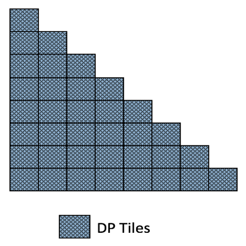
(a) Full Double-Precision (DP).

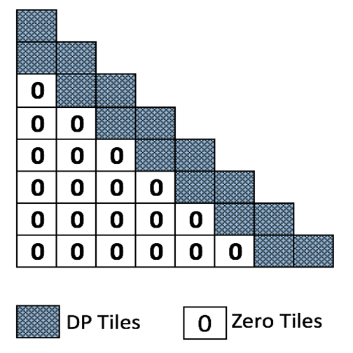
(b) Diagonal Super-Tile (DST).

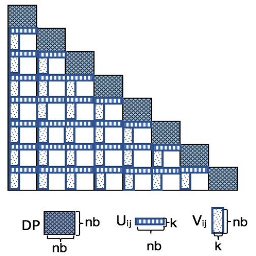
(c) Tile Low-Rank (TLR).

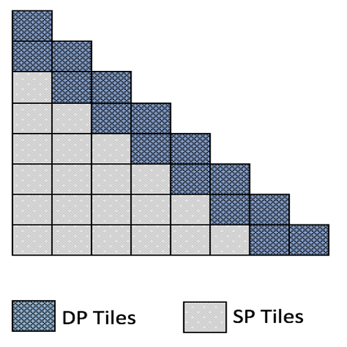
(d) Mixed-Precision (MP).

Figure 1: Four ways of computing the Cholesky-based MLE in ExaGeoStat.

The ExaGeoStat software presents a solution for the exascale computing used in geostatistical modeling and prediction based on the Cholesky factorization to drive the maximum likelihood estimation (MLE). ExaGeoStat currently supports three ways of doing Cholesky factorization to perform the MLE operation, as depicted in Fig. 1(a), Fig. 1(b), and Fig. 1(c). The factorization variant depends on the approximation type applied to the given covariance matrix, i.e., full double-precision dense structure, IndepeNDent blocks/Diagonal Super-Tile (IND/DST) structure, or Tile Low-Rank (TLR) structure. The following subsections give a brief background on each method.

V-A Dense Tile Cholesky Factorization

Fig. 1(a) gives an example of dense computation on a tile-based matrix. All the tiles are represented in double-precision and a set of Level 3 BLAS routines are applied to perform the Cholesky factorization of a given $n\times n$ symmetric, positive-definite matrix. In this paper, we assume that the factorization of $\mathbf{A}$ is presented by $\mathbf{LL}^{\top}$ and $\mathbf{L}$ is an $n\times n$ real lower triangular matrix with positive diagonal elements.

V-B Diagonal Super-Tile (DST) Cholesky Factorization

Covariance tapering is commonly used to approximate the covariance matrix from geostatistics applications by ignoring the correlation with the very far locations [12, 33]. In [34], a tapering algorithm is proposed by setting the correlation between any two far locations $i$ and $j$ equals to zero. This method has been called in statistics as Independent blocks method (IND). The blocks represent different parts of the whole geographical area with maximum dimension equals to the maximum distance between two correlated locations. In [32], we have implemented the IND method by depending on the diagonal elements where the maximum distance can be represented by the number of in-used diagonal tiles. We have called this implementation as the Diagonal Super-Tile (DST) method. Fig. 1(b) gives an example of the DST method where two diagonal tiles are represented in full precision and the other tiles are set to zeros.

Although the IND/DST approach seems impractical in many cases, since it ignores the existing relation between some of the spatial locations; in some cases, an IND/DST approach can be better than sophisticated likelihood approximation methods such as low-rank methods [5], for instance, when observations are dense enough and with low noise effects on the correlations between existing spatial locations. In general, an IND/DST approach can be used to reduce the space and computing complexity of dense computations, as long as it achieves the required accuracy.

V-C Tile Low-Rank (TLR) Cholesky Factorization

Low-rank approximation is a common way to approximate geostatistics covariance matrices [6]. In [35], we have leveraged ExaGeoStat to support Tile Low-Rank (TLR) approximation. The TLR solution depends on exploiting the data sparsity of the given covariance matrix by compressing the off-diagonal tiles up to a certain accuracy level. In TLR approximation, the diagonal tiles are kept as dense while the Singular Value Decomposition (SVD) technique is used to approximate the off-diagonal tiles. Each off-diagonal tile is represented by two matrices $\mathbf{U}$ and $\mathbf{V}$ representing the most significant $k$ singular values and their associated left and right singular vectors, respectively. $k$ is the actual rank of each tile. In general, variables ranks are expected across different matrix tiles. In the case of low accuracy level, small ranks lead to low memory footprint while in the case of high accuracy level, large ranks lead to high memory footprint.

Fig. 1(c) gives an example of applying TLR to a given covariance matrix. Each off-diagonal tile $(i,j)$ is represented by the product of $U_{ij}$, with size $k\times nb$ and $V_{ij}$ with size $nb\times k$, where $nb$ represents the tile size. $nb$ should be tuned in different hardware architectures to obtain the best performance since it corresponds to the trade-off between arithmetic intensity and degree of parallelism.

VI Mixed-precision Cholesky Factorization

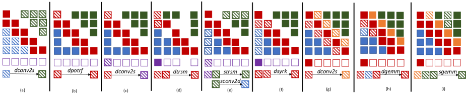
Figure 2: Unrolling the first outer loop iteration of Algorithm 1 with a $5\times 5$ tile matrix size and a diagonal thickness set to 2.

The Cholesky factorization represents one of the most time-consuming operations, when computing the likelihood function given by equation 2. In geostatistics applications, a double-precision arithmetic is usually required to satisfy the desired accuracy level [32, 35]. Assuming an appropriate ordering of the spatial locations, the covariance matrix from those applications has the most valuable information around the diagonal elements of the matrix. The closest locations to a certain location are more correlated to this location, in comparison with far locations. Thus, some methods have proposed to ignore the relation between far locations by ignoring their impact on the covariance matrix, i.e., set to zero [33].

In this paper, we propose a mixed-precision Cholesky factorization algorithm based on the tile-based Cholesky factorization algorithm. This algorithm aims at keeping valuable information around the diagonal elements by using a double floating precision in the diagonal elements, and at the same time, representing the off-diagonal elements in single floating precision to accelerate the algorithm execution time while preserving the accuracy required by the application. However, applying a mixed floating precision is a tricky process, since the computation of each tile depends on other tiles with different data format representation.

To compute the Cholesky factorization of a given dense matrix, only the upper or the lower part of the matrix is used to store the output of the operation, i.e., $\mathbf{A}=\mathbf{LL}^{\top}$. Our proposed implementation uses the other part of the matrix to store the single-precision representation of the matrix tiles, and recalls them when needed. For the diagonal tiles, a tile vector of size $n\times nb$ is required to store the single-precision representation of these tiles.

VII Implementation Details

Algorithm 1 shows the proposed mixed-precision algorithm. A symmetric positive-definite matrix $\bf A$, and the required accuracy level $diag\_thick$ are the two required inputs to the algorithm. The accuracy level represents the number of the diagonal tiles that are represented as double-precision while the remaining off-diagonal tiles are represented in single-precision. Fig. 1(d) shows an example of a mixed-precision data formatting with diagonal thickness = 2 while Fig. 2 gives a step-by-step example of Algorithm 1 using a $5\times 5$ matrix and two double-precision diagonal tiles.

Algorithm 1 Mixed-precision tile Cholesky factorization (lower triangular case)

1:Input: A symmetric positive definite matrix $\bf A$, and the accuracy level $diag\_thick$.

2:for i=1,2,...,p do

3:    for j=i+$diag\_thick$,...,p do

4:        $\bf{A}_{ji}$ $\leftarrow$ dlag2s($\bf{A}_{ij}$)

5:    end for

6:end for

7:for k=1,2,...,p do

8:    $\bf{A}_{kk}$ $\leftarrow$ dpotrf($\bf{A}_{kk}$)

9:    $\bf{tmp}_{0k}$ $\leftarrow$ dlag2s($\bf{A}_{kk}$)

10:    for i=k+1,...,p do

11:        if |m-k| < $diag\_thick$  then

12:           $\bf{A}_{ik}$ $\leftarrow$ dtrsm($\bf{A}_{kk}$,$\bf{A}_{ik}$)

13:        else

14:           $\bf{A}_{ki}$ $\leftarrow$ strsm($\bf{tmp}_{0k}$,$\bf{A}_{ki}$)

15:           $\bf{A}_{ik}$ $\leftarrow$ sconv2d($\bf{A}_{ki}$)

16:        end if

17:    end for

18:    for j=k+1,...,p do

19:        $\bf{A}_{jj}$ $\leftarrow$ dsyrk($\bf{A}_{jk}$,$\bf{A}_{jj}$)

20:        if |k-j| < $diag\_thick$  then

21:           $\bf{A}_{kj}$ $\leftarrow$ dconv2s($\bf{A}_{jk}$)

22:        end if

23:        for i=j+1,...,r do

24:           if |m-k| < $diag\_thick$  then

25:               $\bf{A}_{ij}$ $\leftarrow$ dgemm($\bf{A}_{ik}$,$\bf{A}_{jk}$,$\bf{A}_{ij}$)

26:           else

27:               $\bf{A}_{ji}$ $\leftarrow$ sgemm($\bf{A}_{ki}$,$\bf{A}_{kj}$,$\bf{A}_{ji}$)

28:           end if

29:        end for

30:    end for

31:end for

The algorithm begins by converting all the off-diagonal tiles to a single-precision format using $dconv2s$ kernel, and stores the results to the upper triangular part of the matrix (i.e., assuming lower triangular Cholesky factorization is applied) (lines 2-6). The conversion includes a transpose operation to the selected tile $(i,j)$. This step is also shown by Fig. 2(a). In line 8, a double-precision Cholesky factorization is applied to the diagonal tile ($k$, $k$) (Fig. 2(b)). This diagonal tile is used to perform some single-precision operations on the tiles at the same column $k$. Thus, a single-to-double conversion operation $sconv2d$ is applied to the ($k$, $k$) tile, and the output is stored in a temporary vector $tmp$ (line 9 and Fig. 2(c)). In lines 10-17, $trsm$ operation is applied to all the tiles of column $k$. This operation can be a single or double-precision based on the location of the target tile. The condition statement in line 11 is used to determine the required precision for the $trsm$ operation. If the ($i$, $k$) tile is a diagonal tile from the definition of the diagonal thickness, a $dtrsm$ operation is then applied (Fig. 2(d)), otherwise, a $strsm$ operation is applied to the single-precision tiles of ($k$, $k$) stored at tile ($0$, $k$) in vector $tmp$ and the ($k$, $i$) tile (Fig. 2 (e)). In the case of a single-precision, the $sconv2d$ operation should be applied to update the value of the double tile. In line 19, a $dsyrk$ operation is applied to the diagonal tile ($j$, $j$) (Fig. 2 (f)). In lines 20-21, all the double-precision tiles except the diagonal tiles ($j$, $j$) are converted to single-precision (Fig. 2 (g)). In lines 23-29, a $dgemm$ operation is applied if the ($i$, $j$) tile is a double-precision tile (Fig. 2(h)), otherwise, a $sgemm$ operation is applied (Fig. 2(i)).

VIII Experimental Results

This section presents the evaluation of the proposed mixed-precision versus the full double-precision Cholesky algorithm. The evaluation involves assessing the performance of the MLE algorithm on heterogenous shared-memory, and distributed-memory systems. The assessment of the accuracy involves the estimation of the MLE model parameters and the Prediction Mean Square Error (PMSE), in the context of climate/weather applications using both synthetic and real datasets.

VIII-A Hardware and Software Platform

Our experiments were performed on various hardware architectures. For the shared-memory systems performance assessment, we used two Intel processors, a 18-core dual-socket Intel Haswell chip and a 28-core dual-socket Intel Skylake chip. For the heterogeneous shared-memory (CPU/GPU) systems performance assessment, we used three Intel processors equipped with different GPUs accelerators, a 14-core dual-socket Intel Broadwell chip equipped with a Nvidia Tesla K80 Kepler GPU. a 18-core dual-socket Intel Haswell chip equipped with a Nvidia Tesla P100 Pascal GPU, and a 20-core dual-socket Intel Skylake chip equipped with a Nvidia Tesla V100 Volta GPU, For the distributed memory assessment, we used Shaheen-II, a Cray XC40 system with 6174 compute nodes based on dual-socket 16-core Intel Haswell processors running at 2.3 GHz. Each node has a 128 GB of DDR4 memory. The Shaheen-II has a total of 790 TB of aggregate memory.

Our code was compiled with gcc v5.5.0 and linked against the Chameleon library with HWLOC v1.11.8, StarPU v1.2.4, Intel MKL 2018, GSL v2.4, CUDA v9.0, NLopt v2.4.2 optimization libraries, HDF5 v1.10.1, and NetCDF v4.5.0. Our code will be integrated soon to the ExaGeoStat software.

VIII-B Experimental Testbed Datasets

A set of synthetic datasets and one real dataset were used to evaluate the proposed algorithm. In the ensuing subsections, we provide more details about these datasets.

VIII-B1 Synthetic Datasets

ExaGeoStat provides an internal data generator to simulate synthetic geostatistical data, based on the Matérn covariance function. The synthetic data generation process includes two main operations. First, a set of random 2D irregular spatial locations were generated between $]0,1[$. Second, an initial parameter vector $\boldsymbol{\theta_{0}}$ was used to generate a set of $\boldsymbol{Z}$ measurement vectors associated with the generated locations. More details on the ExaGeoStat data generator tool can be found in [32].

VIII-B2 Real Dataset

we also selected a real geostatistical dataset, the wind speed dataset, coming from the Middle East region to assess our proposed algorithm. Wind speed is a result of changing temperature through the air. The movements of the air from high-pressure to low-pressure layers, or vice versa, impact on the wind speed measurements. The importance of wind speed, as one of the weather components, comes from the fact that it generally affects different activities related to both air and maritime transportation. Additionally, various construction activities from airports to small houses can be impacted by the speed and direction of the wind.

The target dataset was generated using WRF (WRF-ARW) software [36]. The dataset was generated over the Arabian Peninsula in the Middle-East region. Daily data are available for over 37 years; Each data file represents 24 hours measurements of wind speed recorded hourly on 17 different layers. In our case, we picked up one dataset on September 1st, 2017 at time 00:00 AM on a 10-meter distance above the ground (i.e., layer 0). No special restriction is applied to the chosen data. We only select an example to show the effectiveness of our proposed mixed-precision method, but may easily consider extending the datasets.

Fig. 3 shows the wind speed data where the locations were divided into four subregions (i.e., 1, 2, 3, and 4). Each region has approximately $250K$ locations. We choose to divide the dataset into four regions to avoid the non-stationarity exhibition, and to provide four different regions to properly assess the accuracy of our method using different model parameters.

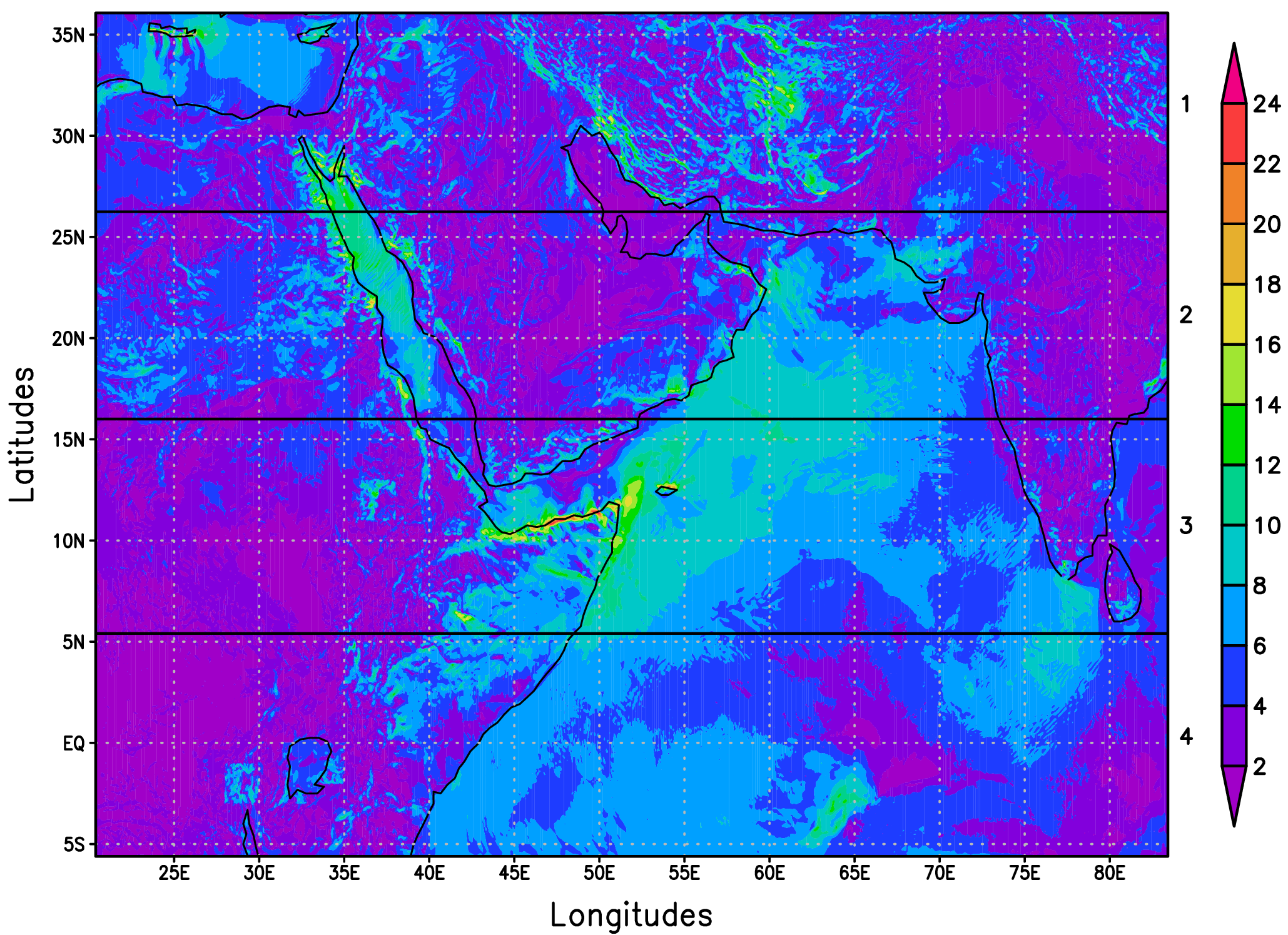
Figure 3: An example of climate/weather geostatistics real data from the Middle East (wind speed data).

VIII-C Mixed Precision MLE Performance Evaluation

In this section, we provide a set of experiments to evaluate the performance of the proposed mixed-precision, in comparison with the full double-precision Cholesky algorithm in the context of the MLE operation. We report the results on heterogenous shared-memory, and distributed-memory systems. The reported time is the average time of one evaluation of the likelihood function. All the plots display how the proposed mixed-precision algorithm outperforms the full double-precision algorithm on different architectures. All figures use different variants of the MLE algorithm. Here, we use DP to represent the pure double-precision arithmetic method, and DP($x\%$)-SP($y\%$) to represent the mixed-precision method where $x\%$ represents the amount of the diagonal tiles that manipulates double-precision and $y\%$ is the amount of the off-diagonal tiles that operates on single-precision.

VIII-C1 Homogeneous Shared-Memory Architectures

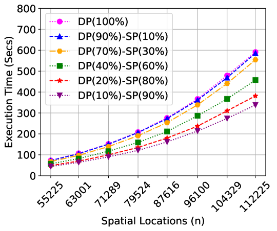
(a) Intel Haswell (36-core).

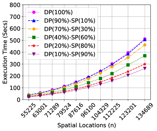
(b) Intel Skylake (56-core).

Figure 4: Execution time per iteration on Intel shared-memory architectures.

we performed the performance analysis of the mixed-precision MLE method on two recent Intel shared-memory architectures, Intel Haswell and Intel Skylake processors, over different problem size up to $\sim 134K$ spatial locations as shown in Fig. 4. The x-axis represents the number of spatial locations $n$, and the y-axis represents the execution time per iteration in seconds. We reported the execution time to show the performance improvement accomplished by the mixed-precision method.

Fig. 4(a) shows the average execution time on a 36-core Intel Haswell processor for different mixed-precision configurations. As shown, the elapsed time for the mixed-precision method with different accuracy levels outperforms the DP(100%) variant. The average obtained speedup of using DP(10%)-SP(90%) variant compared to DP(100%) across different $n$ sizes is about $1.71X$. This speedup decreases when the number of diagonal DP tiles increases, i.e., the increase of the DP diagonal tiles, and the decrease of the SP off-diagonal tiles. The same observation can be made for the Intel Skylake processor in Fig. 4(b) where the average speedup of DP(10%)-SP(90%) variant compared to the DP(100%) is about $1.84X$. In general, it is utmost importance to tune the tile size $nb$ for achieving high performance when running in mixed-precision or full accuracy mode. For both processors, we have used $nb=960$ to achieve the best performance.

Obviously, from the two figures, the average execution time has an inverse proportion with the obtained accuracy at the end. This behavior is expected since using more single-precision tiles should reduce the execution time and at same the time should decrease the estimation accuracy. In section VIII-D, we performed a set of experiments on synthetic datasets and real datasets to show the estimation and the prediction accuracy difference between different mixed-precision variants and the double-precision method.

VIII-C2 Heterogeneous Shared-Memory Architectures

we estimated the average execution time of the likelihood evaluation function, using shared-memory systems equipped with GPU accelerators. The overall execution time on CPU/GPU systems involving both the computation time and the data movement time from the CPU memory to the GPU memory or vice versa. Thus, in our study, we estimated the total execution time and the required data movement for both the double-precision and mixed-precision methods.

Fig. 5(a) shows the total execution time, using an Intel Broadwell equipped with a Tesla K80 Kepler GPU. The average speedup that we obtained by the mixed-precision variant DP(10%)-SP(90%) was $1.74X$ with upto $\sim 96K$ spatial locations. The cost of data movement for each mixed-precision variant and for each $n$, in comparison with, the DP arithmetic method, are also shown in Fig. 5(a). The DP(10%)-SP(90%) can reduce the data movement amount upto $50\%$ compared to the DP(100%) variant. For example, with $n=96K$ the data movement cost of the DP(10%)-SP(90%) variant is $1562.07$ GB while the DP(100%) variant requires about $3032.73$ GB. In Fig. 5(b), the obtained speedup by the DP(10%)-SP(90%) variant is $2.18X$ in average compared to the DP(100%) variant using an Intel Haswell equipped with a Tesla P100 Pascal GPU. We found that the difference of data movement between the two variants could reach up to $40\%$. In Fig. 5(c), the speedup reached $1.82X$ whereas the data movement were reduced to as much as $60\%$ of the DP(100%) variant using an Intel Skylake equipped with a Tesla V100 Volta GPU.

In practice, StarPU moves data around much more than expected, due to its aggressive perfecting strategy. Reducing the data transfer amounts between the GPU memory and CPU memory reduces the data communication overhead and increases the overall obtained speedup which can reach more than $2X$ in some cases.

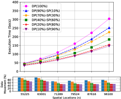
(a) Intel Broadwell w/ K80 GPU.

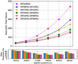
(b) Intel Haswell w/ P100 GPU.

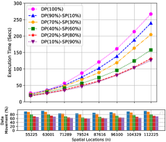
(c) Intel Skylake w/ V100 GPU.

Figure 5: Time and data movement cost per iteration on shared-memory architectures equipped with GPUs.

VIII-C3 Distributed-Memory Systems

we present the performance analysis of the proposed mixed-precision computation on the distributed-memory Shaheen-II Cray XC40 system using a different number of nodes, 64, 128, 256, and 512 (i.e., up to 16384 cores). Fig. 6(a) and Fig. 6(b) show the execution time of different mixed-precision variant compare to the double-precision method. The figures show a speedup upto $1.61X$ and $1.45X$ when using 64 and 128 nodes. Moreover, Fig. 6(c) shows the scalability with different number of nodes, 128, 256, and 512. As also shown in Fig. 6(a) and Fig. 6(b), the mixed-precision method shows a linear scaling behavior with different numbers of nodes, and the gained up speedup for 256, and 512 nodes can reach $1.48X$ and $1.27X$, using the mixed-precision method.

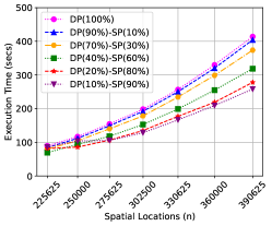
(a) 64 Nodes.

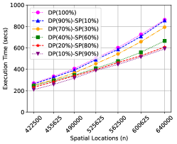
(b) 128 Nodes.

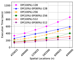
(c) Scalability with different # of nodes.

Figure 6: Execution time per iteration on different number of nodes on Shaheen-II (Cray XC40).

VIII-D MLE Statistical Parameters Estimation/Predictions Accuracy

The experiments in the previous subsection were geared towards the performance evaluation across different hardware architectures. Here, we aim to evaluate the effectiveness of our proposed mixed-precision method for the MLE calculations in terms of parameter vector estimation accuracy and prediction error compared to the DP arithmetic method. To do so, we used both synthetic and real datasets to evaluate the accuracy and to show the effectiveness of the mixed-precision method.

VIII-D1 Synthetic Datasets

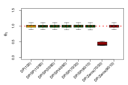
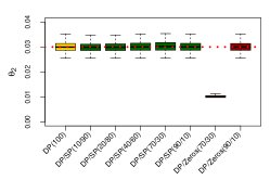
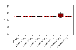
(a) Weak correlation ($\theta_{2}=0.03$).

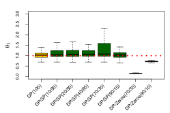
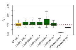
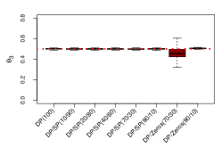
(b) Medium correlation ($\theta_{2}=0.10$).

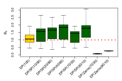
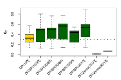
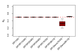
(c) Strong correlation ($\theta_{2}=0.30$).

Figure 7: Parameters estimation boxplots of 40K synthetic datasets using DP, DP(x%)-SP(y%), and DST MLE algorithm. True values of the parameters are represented by red dotted line when estimating the parameter vector.

The MLE operation involves estimating the model parameter vector $\widehat{\boldsymbol{\theta}}=(\theta_{1}$, $\theta_{2}$, $\theta_{3}$) for the underlying data and uses these estimated parameters to predict missing values at other known spatial locations. We performed a set of experiments to evaluate the accuracy of our proposed mixed-precision method for the MLE calculations, based on Monte Carlo simulations. The simulations required the availability of synthetic spatial datasets with different properties to cover different cases that are expected to exist in real data. For instance, $\theta_{2}$, which represents the correlation degree between the given spatial locations, could be weak, medium, or strong. Thus, accuracy verification should involve datasets with different correlation degrees to properly evaluate the proposed MLE computation method.

Recalling section VIII-B1, ExaGeoStat the data generator is used to generate a set of 2D locations with a set of associated $\boldsymbol{Z}$ measurement vectors. We produced a set of $40K$ synthetic datasets that represents the three correlation levels, the weak correlation ($\theta_{2}=0.03$), the medium ($\theta_{2}=0.10$), and the strong ($\theta_{2}=0.30$) correlation levels. For each case, we generated 100 different spatial data (i.e., locations and measurements). We used the DP method, five levels for mixed-precision method, i.e, DP(10%)-SP(90%), DP(20%)-SP(80%), DP(40%)-SP(60%), DP(70%)-SP(30%), DP(90%)-SP(100%), and two levels of the DST method, i.e., DP(70%)-Zero(30%) and DP(90%)-Zero(10%), for accuracy comparison. We have ignored the SP(100%) variant because most of the interactions are captured within the vicinity of the diagonal tiles. Therefore, it is critical to ensure high precision computations (i.e. double-precision) around the diagonal tiles. If single-precision is used instead, the covariance matrix may lose the numerical property of positive definiteness, and the MLE procedure cannot proceed. We also ignores comparisons against TLR because it out of the scope of this paper and it requires a thorough analysis, since it may yield poor results when nuggets (noise) are relatively small and observations are mostly dense [5]. Different computation methods were used to estimate the model parameter vector in order to show that the estimated parameter vector $\widehat{\boldsymbol{\theta}}$ was consistent with the initial parameter vector $\boldsymbol{\theta_{0}}$ that had been used to generate the spatial data.

Fig. 7 shows the estimation accuracy results for the 40K synthetic datasets. The boxplots report the results for 100 different datasets for each correlation case. The experiment involved an estimation of the accuracy of the model parameters for weak, medium, or strong correlations (Fig. 7(a), Fig. 7(b), and Fig. 7(c), respectively) The Prediction Mean Square Error (PMSE) is also shown for each correlation case.

As shown in Fig. 7(a), weak correlated data, i.e., $\theta_{2}=0.03$, required a minimum number of diagonal full-precision tiles, i.e., DP(10%)-SP(90%), to correctly estimate the parameter vector. At the same time, the DST method required at least 90% of the tiles to properly estimate the parameter vector. Fig. 7(b) shows the estimated parameter vector accuracy with medium correlated data, i.e., $\theta_{2}=0.10$. Compared to the weakly correlated, the mixed-precision method is less accurate but is still close to the correct values, whereas the DST method fails to estimate the accurate parameters with both used variants. Fig. 7(c) is related to strongly correlated data, i.e., $\theta_{2}=0.30$. More accuracy is lost when a mixed-precision is used but it is still acceptable, compared with the DST method. These results were expected, because of the tight fit between the spatial data correlation strength and the amount of numeric loss in both mixed-precision and DST methods. A higher correlation strength requires a more accurate representation of the spatial covariance matrix.

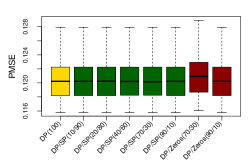
(a) Weak correlation ($\theta_{2}=0.03$).

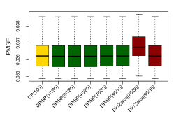
(b) Medium correlation ($\theta_{2}=0.10$).

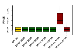
(c) Strong correlation ($\theta_{2}=0.30$).

Figure 8: Prediction Mean Square Error (PMSE) boxplots using $k$-fold cross-validation technique, where $k=10$, of 40K synthetic datasets using DP, DP(x%)-SP(y%), and DST MLE algorithm.

TABLE I: The Matérn covariance parameters estimation and the Prediction Mean Square Error (PMSE) using $k$-fold cross-validation technique, where $k=10$, for $4$ geographical regions of wind speed dataset.

	Matérn Covariance
R	Variance ($\theta_{1}$)						Spatial Range ($\theta_{2}$)						Smoothness ($\theta_{3}$)						Prediction Accuracy (PMSE)
		mixed-precision			DST			mixed-precision			DST			mixed-precision			DST			mixed-precision			DST
		(DP/SP)			(DP/Zero)			(DP/SP)			(DP/Zero)			(DP/SP)			(DP/Zero)			(DP/SP)			(DP/Zero)
	$DP$	$10/90$	$40/60$	$90/10$	$70/30$	$90/10$	$DP$	$10/90$	$40/60$	$90/10$	$70/30$	$90/10$	$DP$	$10/90$	$40/60$	$90/10$	$70/30$	$90/10$	$DP$	$10/90$	$40/60$	$90/10$	$70/30$	$90/10$
R1	8.721	8.695	8.724	8.721	1.115	8.721	32.104	31.986	32.104	32.113	9.990	32.104	1.208	1.210	1.208	1.208	0.983	1.208	0.0361	0.0366	0.0366	0.0361	0.0747	0.0366
R2	12.533	12.548	12.535	12.533	1.589	12.533	27.603	27.640	27.599	27.603	9.990	27.603	1.270	1.269	1.270	1.270	0.970	1.270	0.0571	0.0574	0.0571	0.0571	0.0912	0.0571
R3	10.813	10.870	10.813	10.812	1.230	10.813	19.196	19.241	19.188	19.195	13.880	19.196	1.417	1.417	1.417	1.417	0.538	1.417	0.0612	0.0614	0.0612	0.0606	0.1026	0.0612
R4	12.441	12.440	12.402	12.439	2.452	12.441	19.733	19.732	19.682	19.733	9.990	19.734	1.119	1.119	1.120	1.119	0.875	1.119	0.2098	0.2100	0.2097	0.2098	0.6290	0.0678

VIII-D2 Real Dataset

The estimation operations requires several likelihood function evaluation. Assuming $10^{-3}$ optimization tolerance, we estimate the average number of iterations that requires by each computation variant to convergence. Results showed that high correlated data required more iterations, for both mixed-precision and DST methods, compared with the DP method. Thus, in some cases, the total execution time of the MLE operation using the mixed-precision method exceeded the total time required by the DP arithmetic method. However, the average number of iterations decreased with fewer correlated data.

The PMSE boxplots for three correlation level are shown in Fig. 8. As shown, for our three cases, i.e., strong, medium, and weak correlation, the mixed-precision method has a prediction accuracy close to the DP arithmetic method even with the lowest accurate computation variant, i.e., DP(10%)-SP(90%). However, the DST method only performs well when representing 90% of the tiles in DP representation. We also found the high correlated data to be helpful, in general, to accurately predict missing measurements, but that the accuracy decreased with fewer correlated data.

We validated the accuracy of the proposed mixed-precision method, using the wind dataset. We divided it into four subregions (i.e., 1, 2, 3, and 4) to give more examples to validate our accuracy. Each region has approximately $250K$ locations. Table I reports the complete results of the estimation accuracy besides the prediction error of each computation variant of DP, mixed-precision, and DST methods. The prediction was estimated using the k-fold cross-validation technique, for k=10, to validate the prediction accuracy using different synthetic dataset sizes. The total number of missing values equals to n=k (i.e., subsample size).

Results showed that, across all the regions, all the mixed-precision variants achieved high accuracy estimation levels, equal or at least very close to the estimation achieved by the DP arithmetic method. For the DST method, only DP(90%)/Zero(10%) correctly estimated the parameters of the model. Accordingly, the prediction accuracy of all mixed precision variants were close to the DP prediction accuracy, whereas only DST (DP90%)/Zero(10%) could reach the same prediction accuracy level for all the regions. We also observed that with highly correlated data (i.e., Region 1 and 2), the mixed-precision method required a larger number of iterations to reach convergence, compared with the DP arithmetic method. This number of iterations decreased with the usage of more DP tiles in the diagonal. With fewer correlated data (i.e., regions 3, and 4), the number of iterations was almost the same as the DP arithmetic method.

IX Conclusion and Future Work

Maximum Likelihood Evaluation (MLE) can be used to build a statistical model of a given set of spatial locations and observations, by estimating the more accurate model parameter values that maximize the likelihood that the given observations come from a distribution with these parameter values. In Geostatistics applications, the MLE operation involves building a covariance matrix which requires $O(n^{3})$ floating point operators and an $O(n^{2})$ memory space to be handled in dense format. The Cholesky factorization is the most time-consuming operation in MLE computation. Thus, reducing the complexity of performing it is a necessity to speedup the whole operation especially in large-scale executions. This paper highlights a novel mixed-precision approach for the Cholesky factorization algorithm. The application covariance matrix is built in order for double-precision and single-precision arithmetics to be applied to diagonal tiles and off-diagonal-tiles, respectively. The new implementation provided up to 1.6X performance speedup on massively parallel architectures while maintaining the accuracy necessary for modeling and prediction.

In the paper, we propose an empirical approach and ensure numerical accuracy since the computed ratio of DP/SP is application-dependent. In future work, a more systematic approach can take into account the distance between locations and switch to lower precision beyond a certain distance threshold. We also plan to extend the proposed mixed-precision approach to have three precision layers, i.e., half-precision, single-precision, and double-precision. In this case, we will gain more speedup by ignoring the accuracy in the very far off-diagonal tiles and, hopefully, keep the required accuracy.

Acknowledgement. The authors would like to thank NVIDIA Inc., Cray Inc., and Intel Corp., the Cray Center of Excellence and Intel Parallel Computing Center awarded to the Extreme Computing Research Center (ECRC) at KAUST. For computer time, this research used GPU-based systems as well as Shaheen supercomputer hosted at the Supercomputing Laboratory at King Abdullah University of Science and Technology (KAUST).

[Notes]

References

- [1] M. Asch, T. Moore, R. Badia, M. Beck, P. Beckman, T. Bidot, F. Bodin, F. Cappello, A. Choudhary, B. de Supinski, E. Deelman, J. Dongarra, A. Dubey, G. Fox, H. Fu, S. Girona, W. Gropp, M. Heroux, Y. Ishikawa, K. Keahey, D. Keyes, W. Kramer, J.-F. Lavignon, Y. Lu, S. Matsuoka, B. Mohr, D. Reed, S. Requena, J. Saltz, T. Schulthess, R. Stevens, M. Swany, A. Szalay, W. Tang, G. Varoquaux, J.-P. Vilotte, R. Wisniewski, Z. Xu, and I. Zacharov, “Big data and extreme-scale computing: Pathways to convergence-toward a shaping strategy for a future software and data ecosystem for scientific inquiry,” The International Journal of High Performance Computing Applications, vol. 32, pp. 435–479, 2018.
- [2] “NVIDIA Tensor Cores,” https://www.nvidia.com/en-us/data-center/tensorcore/, 2019, [Online; accessed June 2019].
- [3] “Google Tensor Processing Unit (TPU),” https://cloud.google.com/tpu/, 2019, [Online; accessed June 2019].
- [4] W. Joubert, D. Weighill, D. Kainer, S. Climer, A. Justice, K. Fagnan, and D. Jacobson, “Attacking the Opioid Epidemic: Determining the Epistatic and Pleiotropic Genetic Architectures for Chronic Pain and Opioid Addiction,” in Proceedings of the International Conference for High Performance Computing, Networking, Storage, and Analysis, ser. SC ’18. Piscataway, NJ, USA: IEEE Press, 2018, pp. 57:1–57:14.
- [5] M. Stein, “Limitations on low rank approximations for covariance matrices of spatial data,” Spatial Statistics, vol. 8, pp. 1–19, 2014.
- [6] W. Hackbusch, “A sparse matrix arithmetic based on -matrices. part i: Introduction to -matrices,” Computing, vol. 62, no. 2, pp. 89–108, 1999. [Online]. Available: http://dx.doi.org/10.1007/s006070050015
- [7] Y. Sun, B. Li, and M. G. Genton, “Geostatistics for large datasets,” in Advances and challenges in space-time modelling of natural events. Springer, 2012, pp. 55–77.
- [8] E. Agullo, J. Demmel, J. Dongarra, B. Hadri, J. Kurzak, J. Langou, H. Ltaief, P. Luszczek, and S. Tomov, “Numerical Linear Algebra on Emerging Architectures: The PLASMA and MAGMA projects,” in Journal of Physics: Conference Series, vol. 180, 2009.
- [9] C. Augonnet, S. Thibault, R. Namyst, and P.-A. Wacrenier, “Starpu: a unified platform for task scheduling on heterogeneous multicore architectures,” Concurrency and Computation: Practice and Experience, vol. 23, no. 2, pp. 187–198, 2011.
- [10] S. Banerjee, A. E. Gelfand, A. O. Finley, and H. Sang, “Gaussian predictive process models for large spatial data sets,” Journal of the Royal Statistical Society: Series B (Statistical Methodology), vol. 70, no. 4, pp. 825–848, 2008.
- [11] N. Cressie and G. Johannesson, “Fixed rank kriging for very large spatial data sets,” Journal of the Royal Statistical Society: Series B (Statistical Methodology), vol. 70, no. 1, pp. 209–226, 2008.
- [12] C. G. Kaufman, M. J. Schervish, and D. W. Nychka, “Covariance tapering for likelihood-based estimation in large spatial data sets,” Journal of the American Statistical Association, vol. 103, no. 484, pp. 1545–1555, 2008.
- [13] B. Sinopoli, L. Schenato, M. Franceschetti, K. Poolla, M. I. Jordan, and S. S. Sastry, “Kalman filtering with intermittent observations,” IEEE transactions on Automatic Control, vol. 49, no. 9, pp. 1453–1464, 2004.
- [14] J. M. Ver Hoef, N. Cressie, and R. P. Barry, “Flexible spatial models for kriging and cokriging using moving averages and the fast fourier transform (fft),” Journal of Computational and Graphical Statistics, vol. 13, no. 2, pp. 265–282, 2004.
- [15] Y.-J. Kim and C. Gu, “Smoothing spline gaussian regression: more scalable computation via efficient approximation,” Journal of the Royal Statistical Society: Series B (Statistical Methodology), vol. 66, no. 2, pp. 337–356, 2004.
- [16] A. Litvinenko, Y. Sun, M. G. Genton, and D. E. Keyes, “Likelihood approximation with hierarchical matrices for large spatial datasets,” Computational Statistics & Data Analysis, vol. 137, pp. 115–132, 2019.
- [17] A. Aminfar, S. Ambikasaran, and E. Darve, “A fast block low-rank dense solver with applications to finite-element matrices,” Journal of Computational Physics, vol. 304, pp. 170–188, 2016.
- [18] P. Ghysels, X. S. Li, F.-H. Rouet, S. Williams, and A. Napov, “An efficient multicore implementation of a novel hss-structured multifrontal solver using randomized sampling,” SIAM Journal on Scientific Computing, vol. 38, no. 5, pp. S358–S384, 2016.
- [19] S. Börm and S. Christophersen, “Approximation of integral operators by green quadrature and nested cross approximation,” Numerische Mathematik, vol. 133, no. 3, pp. 409–442, 2016.
- [20] D. Sushnikova and I. Oseledets, “Preconditioners for hierarchical matrices based on their extended sparse form,” Russian Journal of Numerical Analysis and Mathematical Modelling, vol. 31, no. 1, pp. 29–40, 2016.
- [21] G. Pichon, E. Darve, M. Faverge, P. Ramet, and J. Roman, “Sparse supernodal solver using block low-rank compression,” in 2017 IEEE International Parallel and Distributed Processing Symposium Workshops (IPDPSW). IEEE, 2017, pp. 1138–1147.
- [22] K. Akbudak, H. Ltaief, A. Mikhalev, A. Charara, A. Esposito, and D. Keyes, “Exploiting data sparsity for large-scale matrix computations,” in European Conference on Parallel Processing, 2018, pp. 721–734.
- [23] P. D. Düben, H. McNamara, and T. N. Palmer, “The use of imprecise processing to improve accuracy in weather & climate prediction,” Journal of Computational Physics, vol. 271, pp. 2–18, 2014.
- [24] T. Thornes, P. Düben, and T. Palmer, “On the use of scale-dependent precision in earth system modelling,” Quarterly Journal of the Royal Meteorological Society, vol. 143, no. 703, pp. 897–908, 2017.
- [25] L. Gan, H. Fu, W. Luk, C. Yang, W. Xue, X. Huang, Y. Zhang, and G. Yang, “Accelerating solvers for global atmospheric equations through mixed-precision data flow engine,” in 2013 23rd International Conference on Field programmable Logic and Applications. IEEE, 2013, pp. 1–6.
- [26] A. Buttari, J. Dongarra, J. Langou, J. Langou, P. Luszczek, and J. Kurzak, “Mixed Precision Iterative Refinement Techniques for the Solution of Dense Linear Systems,” The International Journal of High Performance Computing Applications, vol. 21, no. 4, pp. 457–466, 2007.
- [27] A. Haidar, S. Tomov, J. Dongarra, and N. J. Higham, “Harnessing GPU Tensor Cores for Fast FP16 Arithmetic to Speed Up Mixed-precision Iterative Refinement Solvers,” in Proceedings of the International Conference for High Performance Computing, Networking, Storage, and Analysis, ser. SC ’18. NJ, USA: IEEE Press, 2018, pp. 47:1–47:11.
- [28] T. Kurth, S. Treichler, J. Romero, M. Mudigonda, N. Luehr, E. Phillips, A. Mahesh, M. Matheson, J. Deslippe, M. Fatica, Prabhat, and M. Houston, “Exascale deep learning for climate analytics,” in Proceedings of the International Conference for High Performance Computing, Networking, Storage, and Analysis, ser. SC ’18. Piscataway, NJ, USA: IEEE Press, 2018, pp. 51:1–51:12.
- [29] H. Ltaief, A. Charara, D. Gratadour, N. Doucet, B. Hadri, E. Gendron, S. Feki, and D. Keyes, “Real-Time Massively Distributed Multi-object Adaptive Optics Simulations for the European Extremely Large Telescope,” in 2018 IEEE International Parallel and Distributed Processing Symposium (IPDPS), May 2018, pp. 75–84.
- [30] H. Ltaief, P. Luszczek, and J. Dongarra, “Solving the generalized symmetric eigenvalue problem using tile algorithms on multicore architectures,” International Conference on Parallel Computing, 2011.
- [31] D. Rick, “Deriving the haversine formula,” in The Math Forum, April, 1999.
- [32] S. Abdulah, H. Ltaief, Y. Sun, M. G. Genton, and D. E. Keyes, “Exageostat: A high performance unified software for geostatistics on manycore systems,” IEEE Transactions on Parallel and Distributed Systems, vol. 29, no. 12, pp. 2771–2784, 2018.
- [33] M. Stein, “Statistical properties of covariance tapers,” Journal of Computational and Graphical Statistics, vol. 22, no. 4, pp. 866–885, 2013.
- [34] H. Huang and Y. Sun, “Hierarchical low rank approximation of likelihoods for large spatial datasets,” Journal of Computational and Graphical Statistics, vol. 27, no. 1, pp. 110–118, 2018.
- [35] S. Abdulah, H. Ltaief, Y. Sun, M. G. Genton, and D. E. Keyes, “Parallel approximation of the maximum likelihood estimation for the prediction of large-scale geostatistics simulations,” in 2018 IEEE International Conference on Cluster Computing. IEEE, 2018, pp. 98–108.
- [36] W. C. Skamarock, J. B. Klemp, J. Dudhia, D. O. Gill, D. M. Barker, W. Wang, and J. G. Powers, “A description of the advanced research WRF version 2,” National Center For Atmospheric Research Boulder Co Mesoscale and Microscale Meteorology Div, Tech. Rep., 2005.
[Notes]