Combined Centrality Measures for an Improved Characterization of Influence Spread in Social Networks

Abstract

Influence Maximization (IM) aims at finding the most influential users in a social network, i. e., users who maximize the spread of an opinion within a certain propagation model. Previous work investigated the correlation between influence spread and nodal centrality measures to bypass more expensive IM simulations. The results were promising but incomplete, since these studies investigated the performance (i. e., the ability to identify influential users) of centrality measures only in restricted settings, e. g., in undirected/unweighted networks and/or within a propagation model less common for IM.

In this paper, we first show that good results within the Susceptible-Infected-Removed (SIR) propagation model for unweighted and undirected networks do not necessarily transfer to directed or weighted networks under the popular Independent Cascade (IC) propagation model. Then, we identify a set of centrality measures with good performance for weighted and directed networks within the IC model. Our main contribution is a new way to combine the centrality measures in a closed formula to yield even better results. Additionally, we also extend gravitational centrality (GC) with the proposed combined centrality measures. Our experiments on 50 real-world data sets show that our proposed centrality measures outperform well-known centrality measures and the state-of-the art GC measure significantly. social networks, influence maximization, centrality measures, IC propagation model, influential spreaders

1 Introduction

Context– Online Social Networks (OSNs) are platforms where many people are connected to each other, e. g., due to their friendship or due to sharing similar opinions [1, 2]. In recent years, with the expansion of OSNs, modeling and analyzing the spread of an impact on the network (opinion, information, unwanted content, viruses, etc.) has gained importance [3, 4]. Deeper insights into impact propagation and key players in this process can be very beneficial, e. g., by maximizing the spread of an advertisement [5, 6] or by preventing the (typically rapid) spread of a rumor, virus, or epidemic [7, 8].

Finding the key players is formalized as the Influence Maximization (IM) problem, which asks for the set of $k$ nodes with the highest number of influenced users (i. e., the influence spread) [9]. How the influence spreads, is captured by a so-called propagation model, also see Section 2.3. It has been shown that the IM problem is $\mathcal{NP}$-hard under most propagation models [10]. Thus, when addressing IM in practice, one usually opts for heuristic approaches or even proxies such as centrality measures. Centrality measures indicate the importance of a node in the network via its position [11, 12]; numerical values yield a partial order and thus a node ranking. Such a ranking is an important basis for seeding the key players in many IM algorithms [10, 13, 14]. Also, numerous recent works investigated the correlation between centrality values of nodes and their influence capability [2, 15, 16, 17, 18, 19, 20] – not only for established measures such as betweenness, closeness or Katz centrality, but also for newly developed centrality measures such as Gravitational Centrality (GC) [15]. In this case the centrality measures act as a proxy, i. e., they indicate the influence capability of a node implicitly. With a good correlation, one may be able to bypass more costly propagation simulations.

Motivation– The propagation model is indeed an integral part of the IM problem which determines the key players – thus, different models may lead to a completely different set of influencers. A centrality measure’s ability to indicate the influence spread capability of a node (i. e., its performance in our context) is affected by the propagation model as well. Indeed, a centrality measure that provides good performance on undirected and unweighted networks under the Susceptible-Infected-Removed (SIR) propagation model [21], may give poor results on directed and weighted networks under the Independent Cascade (IC) model. Most of the established and recently tailored centrality measures, however, have been investigated under the SIR model and similar models such as Susceptible-Infected (SI) only [2, 15, 16, 17, 18, 20, 22]. Most of the recent IM algorithms,in turn, have been developed for Independent Cascade [23, 24, 25, 26, 27, 28] and partly for Linear Threshold [29, 30]. Hence, in this study, we focus on IC propagation and aim at centrality measures that correlate well with the nodes’ influence capabilities under IC.

Contribution and Outline of the Paper– To this end, after preprocessing (Section 3.1), we analyze numerous centrality measures on 50 real-world data sets under the IC model, see Section 3.2. Their performance in terms of correlation to influence spread often differs significantly from their performance in the SIR model. For example, GC’s performance is much worse with IC. This is an important observation since most of the recent centrality measure development studies have been tested under (and partially tuned for) the SIR model [2, 15, 16, 17, 18, 20, 22]. To the best of our knowledge, our study is the most comprehensive one on new centrality measures for the IC model.

We put the best performing centrality measures together as linear combinations of two each; this yields four new combined centrality measures (Section 3.3). To obtain the coefficients of each single measure, we use the correlation between the centrality measure and the real spreading capability.

In addition, we develop new measures based on Gravitational Centrality; instead of the original $k$-shell mass (see Section 2.5 for the definition), we use our combined measures.

Our experimental results (cf. Section 4) show that the proposed combined centrality measures and the modified GC measures outperform the state of the art significantly (the latter being based on GC and some basic centrality measures). Thus, with the proposed measures, one can bypass costlier propagation simulations in the IC model, but still gets highly correlated results.

2 Preliminaries and Related Work

2.1 Notation

We represent a social network by a weighted simple graph $G=\{V,E,w\}$, which is directed unless stated otherwise. $V$ is the set of nodes (individuals), $E$ is the set of edges (relations), and $w:E\rightarrow\mathbb{R}_{>0}$ is the edge weight function.

In our context we usually encounter weighted graphs where the edge weights model the influence diffusion probabilities between neighboring nodes. For an easier distinction, we write $G^{uu}$ for undirected unweighted graphs, $G^{uw}$ for undirected weighted graphs, $G^{du}$ for directed unweighted graphs, and $G^{dw}$ for directed weighted graphs, respectively.

We frequently use the (weighted) adjacency matrix $A$ of $G$, which contains the weight of edge $(u,v)$ in position $(A)_{u,v}$ (often written as $a_{uv}$) and zeros elsewhere. Finally, the $r$-hop neighborhood, $N_{r}(u)$, of a node $u$ is the set of nodes that can be reached from $u$ by traversing at most $r$ edges.

2.2 Influence Maximization in Social Networks

Influence maximization (IM) aims at finding a small subset of nodes that are able to influence as many other nodes as possible in a network [10]. In this context we mean by “$u$ influences $v$” if $u$ passes an opinion/information on to $v$ (possibly indirectly via other nodes) that is accepted by $v$ (and then passed on). There are many algorithmic approaches to address this $\mathcal{NP}$-hard combinatorial optimization problem by selecting (hopefully) very influential seed nodes: various greedy approaches (one-by-one [10], single stage seeding, sequential seeding [31]) as well as metaheuristics such as genetic algorithms, simulated annealing, and swarm intelligence [25, 26, 32, 27, 33].

Regardless of the adopted algorithmic approach, it is rather natural to evaluate the nodes in terms of their influence spread capability – numerical values for this evaluation can then lead to a ranking. Typically, such an evaluation is based on propagation simulations, which are very costly. The results of these simulations depend very much on the propagation model, i. e., how an opinion is passed on (or not) to the neighbors of a node. The two models most relevant for our paper are described next.

2.3 Propagation Models for IM in Social Networks

Propagation (or diffusion) models can be categorized into three main types: (i) Threshold models such as Linear threshold (LT) [34, 35], (ii) cascading models such as Independent cascade (IC) [29], and (iii) epidemic models such as Susceptible-Infected-Removed (SIR) [20]. This paper focuses on IC; since IC can be seen as a variant of SIR, we describe both in some detail and pass over LT.

The SIR model is a general information diffusion model often used in modeling disease spread; each node has three states: susceptible (S), infected (I), and recovered (R). Infections can only happen when an infected node transmits the disease to a neighboring susceptible node. In each discrete time step, the infected nodes can spread the disease with probability $\beta$, then enter the recovered state with another probability. In the context of IM, the information to be spread is the disease in SIR, of course. The original and frequently used SIR model (see for example [21, 36]) does not reflect the behavior of influence spread in OSNs since it assumes one global infection probability, regardless of the node pair involved (although more general SIR variations exist [37, 38], but not in the IM context).

The IC model, our main focus, can be considered as a close relative SIR, though. IC has only two states (active and inactive and thus no recovered state), but also a static (i. e., unchanged over time) $\beta$ value. If a person is influenced by another person, it becomes active. An activated person can influence other persons and cannot return to the inactive state again. The IC model associates with each $e\in E$ a propagation probability $P(e)\in[0,1]$. If we already know sensible values for these probabilities of influence diffusion, then we can use this information. However, if they are unknown, the literature usually resorts to established probability models. So do we: we adopt the Weighted Cascade Setting (WCS) model in which for $e=(u,v)\in E$ one sets $P(e)=1/(\deg^{-}(v))$, where $\deg^{-}(\cdot)$ is the in-degree. WCS is based on the idea that a node’s probability of being influenced is inversely proportional to the number of nodes that may directly influence this node.

Influence diffusion in the IC model works as follows: A set of initially active (= influenced) nodes, the seed nodes, is chosen. Then, within each iteration, all active nodes try to influence all their out-neighbors. To this end, each active node generates a random number $r_{e}\in[0,1]$ per out-edge $e$. If $r_{e}<P(e)$,

then the neighbor at the other end of $e$ is activated. If no new node is activated in an iteration, the propagation process ends. Since the IC model is probabilistic, modeling the propagation needs to be repeated and the expected value of the propagation should be taken. It is usually enough (from an empirical point of view) to repeat the propagation 20 000 times [35].

2.4 Established Centrality Measures

Recall that centrality measures are used to rank nodes based on their position in the graph. This ranking can also be used to seed IM algorithms with very central nodes [3, 15, 16, 17, 18, 19, 20, 35, 39]. Since such a ranking is often much faster to compute, centrality measures have been of high interest in the context of IM. We are interested in measures with high performance, i. e., whose ranking result correlates well with the influence spread of the nodes. After describing established basic measures (see e. g., Newman [21]) first, we review measures created with IM in mind.

Basic local centrality measures are degree and strength centrality. The degree centrality of $u\in V$, $C_{D}(u)$, is the size of $u$’s neighborhood, i. e., the number of $u$’s neighbors. This can be generalized in an analogous manner to in- and out-degree centrality ($C_{ID}(u)$ and $C_{OD}(u)$), respectively, in directed graphs. Strength centrality, $C_{S}(u)$, is just the weighted version of degree centrality: instead of using the neighborhood size, one sums up the weight of all incident edges of $u$. As above, this notion can be generalized easily to in- and out-strength centrality ($C_{IS}(u)$ and $C_{OS}(u)$) in directed graphs, respectively.

One of the global centrality measures is betweenness centrality. It considers a node’s participation in shortest paths:

$$C_{B}(u)={\sum_{s\neq u\neq t\in V}\frac{\sigma_{st}(u)}{\sigma_{st}}},$$ (1)

where $\sigma_{st}$ is the number of all shortest paths between/from $s$ and/to $t$ and $\sigma_{st}(u)$ is the number of shortest paths between/from $s$ and/to $t$ that pass through $u$ as intermediate node. If a node’s betweenness is high, more information is assumed to flow through this node.

Also based on shortest paths is the global measure closeness centrality; it is defined as the reciprocal of the average distance $\operatorname{dist}(\cdot)$ (distance = length of shortest path) to all other nodes. This way, a high closeness value indicates that the corresponding node is located in the center of the graph:

$$C_{C}(u)=\frac{n-1}{\sum_{v\neq u\in V}\operatorname{dist}(u,v)}.$$ (2)

Another global measure is eigenvector centrality. It measures a node’s importance by the importance of its neighbors. More precisely, the centrality value of node $u$ is the $u$th entry of the leading eigenvector $x$ of the adjacency matrix $A$ [21]. Hence: $x_{u}={\lambda_{1}^{-1}\sum_{v=1}^{n}a_{uv}x_{v}},$ where $\lambda_{1}$ is the largest eigenvalue of $A$. Eigenvector centrality should not be applied to directed graphs that are not strongly connected.

We mention Katz centrality as the last global centrality measure:

$$C_{Katz}(u)={\sum_{k=1}^{\infty}\alpha^{k}\sum_{v=1}^{n}(A^{k})_{vu}}.$$ (3)

Here, $0<\alpha<1$ is an attenuation factor to dampen the contribution of the number of walks of length $k$ from $v$ to $u$, $(A^{k})_{vu}$, for larger $k$.

2.5 Recent Centrality Measures for IM Seeding

Additionally, several centrality measures have been developed for or adapted to certain IM propagation models recently – for example gravitational centrality (GC) [15], $C_{GC}$, which is inspired by Newton’s gravity formula:

$$C_{GC}(u)={\sum_{v\in N_{r}(u)}\frac{ks(u)ks(v)}{(\operatorname{dist}(u,v))^{2}}}$$ (4)

Here, $ks(u)$ and $ks(v)$ are the k-shell values of nodes $u$ and $v$, respectively. The k-shell of a graph $G$ is a subgraph that consists of the nodes in the $k$-core but not in the $(k+1)$-core. The $k$-core of $G$, in turn, is the maximal subgraph in which every node has degree at least $k$ [21]. As the original paper [16], we set $r:=3$ for the neighborhood $N_{r}(\cdot)$ in all GC-related measures.

Ma et al. [15] use the SIR epidemic model to investigate the performance of gravitational centrality and an extension of GC, GC+, for IM. They compare its IM performance with established centrality measures such as degree, closeness, betweenness, semi-local centrality, etc. The average performance of the two new measures in terms of ranking correlation and distinction between nodes is slightly better than for established measures; in terms of Kendall $\tau$ correlation (defined in B) results aggregated over nine real-world data sets, the performance of GC and GC+ are $0.83$ and $0.847$, respectively. The performance of semi-local centrality, the best competitor in the study, is $0.821$.

Originally, GC has been developed for undirected and unweighted graphs, but it can be generalized for weighted networks as well [15]. To this end, a partially weighted degree needs to be calculated:

$$k_{i}^{\prime}={\sqrt{k_{i}\sum_{j=1}^{n}a_{ij}}}$$ (5)

Here, $k_{i}$ is the (unweighted) degree of node $i$, so that we take the square root of the product of the unweighted and the weighted degree. Garas et al. [41] normalize the $k_{i}^{\prime}$ values. As we work with directed graphs in which some nodes have out-strength $0$, we adapt their normalization process and do not divide by the minimum value. The experimental results and their interpretation remain unaffected by this change.

From now on, we refer to gravitational centrality for weighted networks as $C_{GC}^{w}$.

Wang et al. [16] recently proposed two extensions of gravitational centrality, $ks_{G}$ and $ks_{G+}$.

$ks_{G}$ modifies the $C_{GC}$ formula by using degree values instead of $ks(v)$ in Eq. (4). $ks_{G+}$ is calculated as sum of all neighbors’ $ks_{G}$ values. The experimental results reveal that the performance of $ks_{G}$ and $ks_{G+}$ is similar to that of $C_{GC}$ in the SIR model.

Other recent developments in the field include BridgeRank [20] and dynamics-sensitive (DS) centrality [18]. BridgeRank is a semi-local measure based on communities and local betweenness values. SIR experiments on four real-world and four synthetic networks [18] have shown that BridgeRank and its variants outperform basic centrality measures. DS, in turn, integrates topological features of the network and the spreading dynamics of the propagation model under consideration. SIR and SI experiments on four real-world networks indicate that DS can outperform basic centrality measures as well.

GC is a rather general framework; different centrality measures can be included, in particular in the numerator. New studies are inspired by GC, e. g., a new $k$-shell hybrid method has been developed for unweighted networks and the SIR model [17]. Their results, if compared to GC, do not significantly outperform the original definition [20, 18, 17], though. Moreover, all studies mentioned in this papragraph work with unweighted and/or undirected networks. Thus, one can still consider GC as state of the art in the field. While an extension to weighted GC has been proposed [15], to the best of our knowledge we provide the first substantial experimental results for its usage in weighted networks.

2.6 Summary

Greedy algorithms as well as metaheuristics compute their seed set based on the fitness of the nodes – in this case the real, simulated or indirectly assumed influence spread capabilities. Using centrality measures as a proxy for that can save a lot of running time – if the correlation between centrality and influence spread is high. As reported in the literature review, most recent works investigated centrality measures under the SIR model and very similar models. Yet, most of the recent IM algorithms have been developed for the Independent Cascade (IC) model (and partly for Linear Threshold). As the performance of a centrality measure depends on the propagation model (among others), good performance on undirected and unweighted networks under the SIR propagation model [15] may not transfer to directed and weighted networks under the IC model. Hence, we aim at new centrality measures with good performance under the (for IM) more popular IC model.

3 Materials and Methods

Our primary assumption is that a high correlation between the centrality scores of one measure and the influence spread can be further improved by combining two measures appropriately. Thus, in this section, we identify centrality measure candidates by exploration and derive new measures, e. g., as linear combinations of two candidates.

3.1 Data Acquisition and Preprocessing

The 50 social networks we use for our study are listed in Table 7 in A. They have been downloaded from the public sources SNAP [42], KONECT [43], and Network Repository [44]. We can use each network in principle in four ways: The undirected networks are made directed by pointing each edge from the node with smaller to the node with higher ID. When considering undirected graphs only, we ignore the direction specified by directed graphs. Similarly, when considering unweighted graphs only, we ignore weights specified by the data sets. On the other hand, when we work with a collection of weighted graphs, we create weighted versions of unweighted data sets by using the WCS model (see Section 2.3 for WCS).

This leads to four data collections that we index according to their type: (i) $G^{uu}$: undirected and unweighted, (ii) $G^{uw}$: undirected and weighted, (iii) $G^{du}$: directed and unweighted, (iv) $G^{dw}$: directed and weighted. We distinguish between four types because not every centrality measure can be computed for all types (without problems). Our main focus is on $G^{dw}$, however, because it is the most relevant input class for IM in social networks.

In the IC model, a high edge weight means a high probability of a node $u$ to be influenced by another node $v$. For closeness and betweenness, however, it means that two nodes are further away. Thus, we invert the edge weights of the graphs as $1/w$ when calculating distance-based centrality measures such as $C_{B}^{uw}$ and $C_{C}^{dw}$.

3.2 Exploratory Experiments

We start by investigating the correlation of single centrality measures and their influence spread. Recall that our plan is to combine the successful ones later on to obtain an even better measure. For all our experiments in this paper, we use NetworKit [45] as network analysis tool. Self-implemented code for the new measures is written in Python 3.

We investigate the following centrality measures on the different graph types as specified: (i) Out-degree in $G^{du}$ ($C_{OD}$), (ii) out-strength in $G^{dw}$ ($C_{OS}$), (iii) betweenness in $G^{uu}$ ($C_{B}^{uu}$), (iv) betweenness in $G^{uw}$ ($C_{B}^{uw}$), (v) outbound closeness in $G^{du}$ ($C_{C}^{du}$), (vi) outbound closeness in $G^{dw}$ ($C_{C}^{dw}$), (vi) eigenvector centrality in $G^{uu}$ ($C_{E}^{uu}$), (vii) Katz (incoming) centrality in $G^{du}$ ($C_{Katz}^{du}$), and (viii) Katz outgoing centrality in $G^{dw}$ ($C_{Katz\rightarrow}^{dw}$). Moreover, since exact betweenness calculations are very time-consuming (even more than simulating influence propagation), we resort to approximations based on the algorithms KADABRA [46] for undirected unweighted graphs and RK for undirected weighted graphs [47] (with $\epsilon=0.1$). For closeness centrality, we use the corresponding approximation algorithm (with $\epsilon=0.1$) in NetworKit, too. Also note that Katz centrality takes incoming edges into account. Yet, on the social networks we use, the direction of the influence is modeled by outgoing edges. That is why we can expect low Katz centrality to co-occur with high influence spread.

The expected influence spread is calculated for the IC model as follows: Each node is selected as single seed, then the propagation based on this seed is run until convergence. This probabilistic process is repeated 20 000 times (as suggested by [35]) per node to account for random fluctuations; the arithmetic mean is used as the influence spread result for that seed node.

Figure 1 displays the simulation results for the network socfb-Howard90. Each point $(x,y)$ represents the centrality score $x$ (usually normalized by the maximum value) vs. its influence spread $y$ for a particular seed. Our visual interpretation is mostly interested in a good distinction between the nodes and a (possibly linear) trend/correlation between centrality and spread.

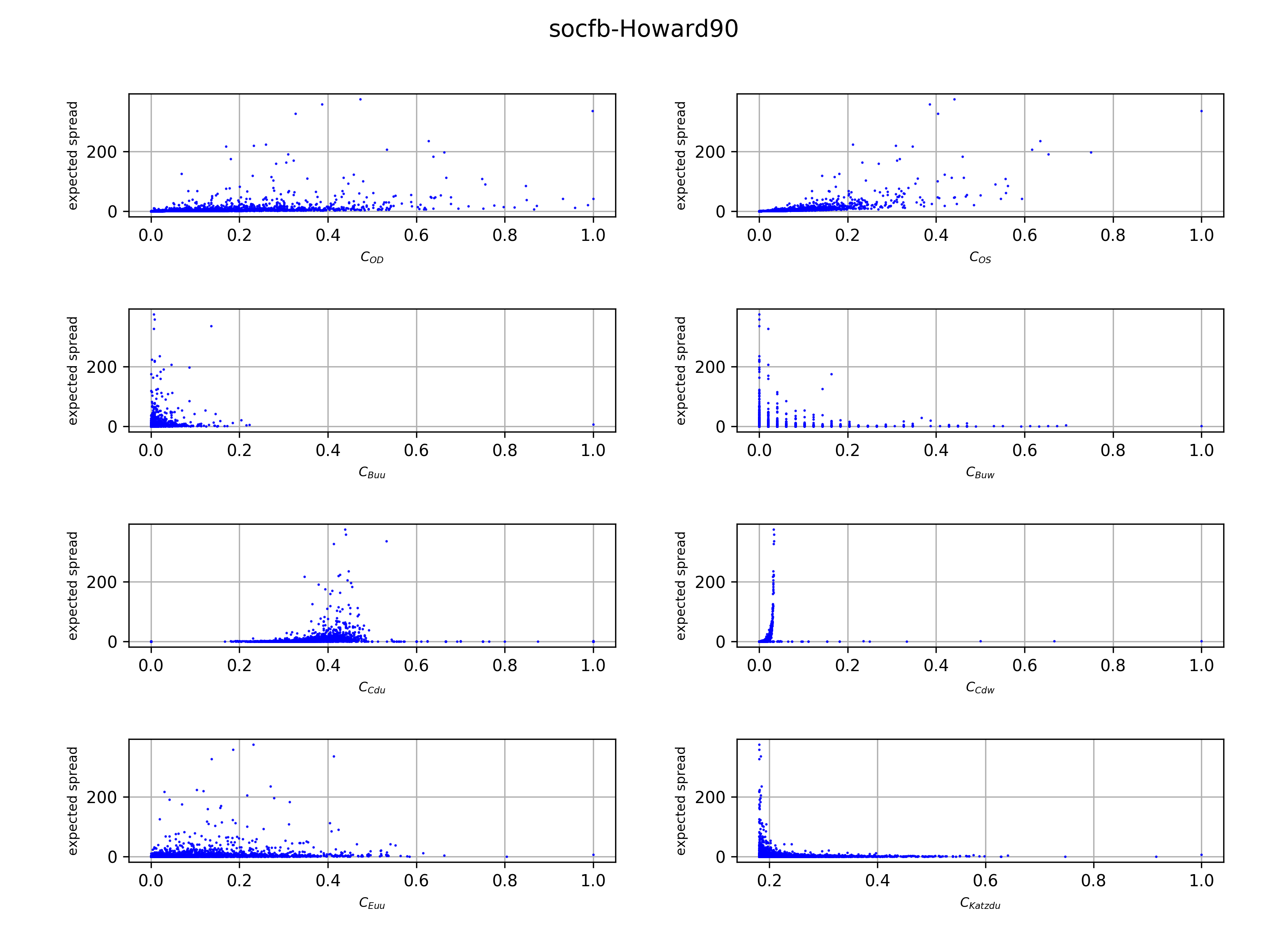
Figure 1: Centrality measure vs. expected spread for the socfb-Howard90 data set.

We observe that the point distributions of $C_{OS}$, $C_{C}^{dw}$, and $C_{Katz}^{du}$ are reasonably spread out. This means that these centrality measures allow a better distinction between nodes in terms of their influence spread capability. $C_{B}^{uw}$, on the other hand, yields values that seem discretized into numerous narrow intervals. These observations provide visual (and thus informal) indication of good and bad ranking monotonicity, respectively; in general terms, ranking monotonicity measures the fraction of (non-)ties in a ranking and thus the ability to distinguish nodes (see Def. 3 in B for a formal definition).

Furthermore, the $C_{OS}$ values increase with the expected spread. While this behavior is not necessarily linear, a trend in the sense of “higher centrality means higher spread” is visible. $C_{OD}$ yields results similar to $C_{OS}$, but the $C_{OS}$ values are more distinguishable. In fact, this trend is a visual indication of a low ranking error, which measures (broadly speaking) how well a ranking $X$ preserves a ranking $Y$ (a more formal description is given as Definition 1 in B). Betweenness, in turn, does not have such a trend; its values are clustered within narrow intervals. As expected, the slope of the $C_{Katz}^{du}$ values is negative; we will account for that later on. To analyze the results not only visually, we proceed with the Kendall $\tau$ ranking correlation coefficient (see Definition 1 in B) for each measure. The numerical results are given in Table 8 in 14. In order to see a measure’s relative performance in comparison with $C_{OD}$, we divide all scores by the $C_{OD}$ results. For a global, aggregate perspective, we provide in the last row the geometric means of these ratios over all data sets. (We use the absolute values of the results in the geometric mean calculation because some results are negative. While this approach may make the means harder to interpret, a close inspection of Table 8 reveals that the qualitative interpretation is not changed.) It is evident from the values that the centrality measures betweenness, closeness, eigenvector, Katz, and wks do not perform well when used alone. Only strength centrality shows a high correlation. Of the global measures, closeness and Katz perform best.

In summary, the best performing local measure is $C_{OS}$. Of the global measures, $C_{C}^{dw}$ and $C_{Katz}^{du}$ seem overall reasonably promising. The other measures’ patterns are not as good or even unclear. Therefore, we proceed with $C_{OS}$, $C_{C}^{dw}$, and $C_{Katz}^{du}$ when creating combined measures; further experiments in the paper will not consider the other basic measures.

3.3 Combined Centrality Measures

Based on the insights above, we proceed by combining different measures into new ones. We aim for a linear combination of a local and a global centrality measure to merge both perspectives of a node, e. g., $SC_{1}:=\gamma\cdot C_{OS}+\delta\cdot\tilde{C}_{C}^{dw}$. Note that we introduce a small change to the closeness values in weighted directed graphs. Since the largest spread is observed for $C_{C}^{dw}$ values between $0.0$ and $0.04$ (with high slope), we modify $C_{C}^{dw}$ in order to match high centrality values with high influence spread:

$$\tilde{C}_{C}^{dw}(u):=\begin{cases}C_{C}^{dw}(u)+1-0.04&\text{if }C_{C}^{dw}(u)\leq 0.04\\ 1-C_{C}^{dw}(u)+0.04&\text{if }C_{C}^{dw}(u)>0.04\end{cases}$$ (6)

To determine the coefficients $\gamma$ and $\delta$ of our linear combination, we make use of the respective correlation strength – the measure with higher strength shall receive a higher coefficient. To this end, let $k(C_{OS})$ and $k(\tilde{C}_{C}^{dw})$ be the geometric mean of the normalized $\tau$ results of $C_{OS}$ and $\tilde{C}_{C}^{dw}$ (see Table 8). This leads to $\gamma:=\frac{k(C_{OS})}{k(C_{OS})+k(\tilde{C}_{C}^{dw})}\approx 0.64$ and $\delta:=\frac{k(\tilde{C}_{C}^{dw})}{k(C_{OS})+k(\tilde{C}_{C}^{dw})}\approx 0.36$. Thus:

$$SC_{1}={0.64\cdot C_{OS}+0.36\cdot\tilde{C}_{C}^{dw}}$$ (7)

As further combinations of a local ($C_{OS}$) and a global (now $C_{Katz}^{du}$) measure, we propose the following group of measures:

$$SK_{1}=C_{OS}+{\frac{C_{OS}}{C_{Katz}^{du}}}$$ (8)

$$SK_{2}=C_{OS}-{\frac{C_{Katz}^{du}}{C_{OS}+C_{Katz}^{du}}}$$ (9)

$$SK_{3}={\frac{C_{OS}}{C_{Katz}^{du}}}$$ (10)

The rationale behind these formulas is the following: In all data sets, the $C_{OS}$ values increase while the expected spread increases; also, in most of the data sets, the $C_{Katz}^{du}$ values decrease while the expected spread increases. Thus, we use $C_{OS}$ as numerator and $C_{Katz}^{du}$ as denominator in $SK_{1}$ and $SK_{3}$. In $SK_{2}$ we use $C_{Katz}^{du}$ as numerator because we subtract the result of the division from $C_{OS}$ to get a positive correlation between $SK_{2}$ and the expected spread.

3.4 Variations of Gravitational Centrality

In addition to the proposed measures above, we create modifications of gravitational centrality (GC). GC is a general framework in which new measures can be integrated easily. To do so, we consider the Kendall $\tau$ correlation results of all the measures presented in Tables 8 and 9. The following measures yield significant results and are proposed for directed and weighted graphs. Hence, shortest path calculations are performed on $G^{dw}$. Also, we invert the edge weights of the graphs as $1/w$ when calculating shortest path lengths for all centrality measures based on GC (incl. $C_{GC}^{w}$). First, let the modified GC using out-degree strength be

$$MGC_{ODS}(i)={\sum_{j\in N_{3}(i)}\frac{ods(i)\cdot ods(j)}{(\operatorname{dist}(i,j))^{2}}},$$ (11)

where $ods(i)=C_{OD}(i)\cdot C_{OS}(i)$ for a node $i\in V$. All other parameters have the same meaning as in Eq. (4). Note that $C_{OD}$ and $C_{OS}$ are basic local measures. Yet, according to our results, they are strong indicators for influence capability of a node on a directed and weighted graph. To (potentially) create an even stronger measure, we propose further variations within the GC formula, here specified for $i\in V$:

$$MGC_{S}(i)={\sum_{j\in N_{3}(i)}\frac{C_{OS}(i)\cdot C_{OS}(j)}{(\operatorname{dist}(i,j))^{2}}},$$ (12)

$$MGC_{SC}(i)={\sum_{j\in N_{3}(i)}\frac{SC_{1}(i)\cdot SC_{1}(j)}{(\operatorname{dist}(i,j))^{2}}},$$ (13)

$$MGC_{SK}(i)={\sum_{j\in N_{3}(i)}\frac{SK_{3}(i)\cdot SK_{3}(i)}{(\operatorname{dist}(i,j))^{2}}},$$ (14)

$$MGC_{wk}(i)={\sum_{j\in N_{3}(i)}\frac{wk(i)\cdot wk(j)}{(\operatorname{dist}(i,j))^{2}}},$$ (15)

where $wk(i)=ods(i)\cdot C_{Katz\rightarrow}^{dw}(i)$.

4 Experimental Results

In this section, we provide and discuss the experimental results of our proposed measures, out-strength, and weighted gravitational centrality ($C_{GC}^{w}$). Our evaluation is based on the assessment of three ranking performance measures: Kendall $\tau$ correlation, ranking error, and ranking monotonicity (for the definitions of these measures, cf. B).

Kendall $\tau$ correlation

Geometric mean values of the normalized Kendall $\tau$ ranking results are shown in Tables 1 and 2 for all proposed centrality measures as well as for $C_{OS}$ and $C_{GC}^{w}$. Detailed results on all data sets are shown in Tables 9 and 10.

Table 1: Geometric means of normalized Kendall $\tau$ results for combined measures

Centrality Measures	$C_{OS}$	$SC_{1}$	$SK_{1}$	$SK_{2}$	$SK_{3}$	$C_{Katz\rightarrow}^{dw}$
Geometric mean	1.29864	1.35576	1.04994	1.28907	1.31493	1.30657

Table 2: Geometric means of normalized Kendall $\tau$ results for modifications of gravitational centrality

Centrality Measures	$C_{GC}^{w}$	$MGC_{ODS}$	$MGC_{S}$	$MGC_{SC}$	$MGC_{SK}$	$MGC_{wk}$
Geometric mean	0.70205	1.38455	1.35513	1.29802	1.31421	1.40721

When inspecting the detailed values, we see that $MGC_{wk}$ has the highest correlation on 43 data sets, $MGC_{ODS}$ has the highest Kendall $\tau$ correlation on six data sets, and $SC_{1}$ performs best only once. If we sort the measures according to the geometric mean results in descending order, the ranking is as follows: $MGC_{wk}$, $MGC_{ODS}$, $SC_{1}$, $MGC_{S}$, $SK_{3}$, $MGC_{SK}$, $C_{Katz\rightarrow}^{dw}$, $C_{OS}$, $MGC_{SC}$, $SK_{2}$, $SK_{1}$, $C_{GC}^{w}$. According to the overall Kendall $\tau$ correlation results, seven of the proposed measures outperform $C_{OS}$, and all of the proposed measures outperform $C_{GC}^{w}$. Note that Ma et al. [15] reported that GC’s performance in terms of Kendall’s $\tau$ is slightly better than degree centrality’s within the SIR model. In our experiments within the IC model, however, GC reaches only 70% of out-degree’s performance.

Ranking error

For the ranking error experiments, we exclude the data sets Moreno highschool, Moreno dutch college, and Moreno seventh grader from the experiments because they have less than 100 nodes and we focus here on the top-$50$. Geometric means of the normalized ranking error $\epsilon$ for the top-$50$ nodes of each measure are shown in Tables 3 and 4. The detailed results on all data sets are shown in Tables 11 and 12.

Table 3: Geometric means of normalized $\epsilon$ for $C_{OS}$, $C_{Katz\rightarrow}^{dw}$, and the proposed combined measures

Data sets	$C_{OS}$	$SC_{1}$	$SK_{1}$	$SK_{2}$	$SK_{3}$	$C_{Katz\rightarrow}^{dw}$
geometric mean	0.47425	0.47453	0.42411	0.43921	0.41501	0.47415

Table 4: Geometric means of normalized $\epsilon$ for modifications of gravitational centrality.

Centrality Measures	$C_{GC}^{w}$	$MGC_{ODS}$	$MGC_{S}$	$MGC_{SC}$	$MGC_{SK}$	$MGC_{wk}$
geometric mean	0.16681	0.08432	0.09198	0.09174	0.09066	0.24280

When inspecting the detailed data, we see that $MGC_{SK}$ has the lowest $\epsilon$ on 20 data sets; $MGC_{ODS}$, in turn, performs best on 18 data sets. Moreover, $MGC_{S}$ and $MGC_{SC}$ have the lowest $\epsilon$ on 12 data set, respectively, whereas $C_{GC}^{w}$ performs best on six data sets. All the measures’ $\epsilon$ values for the socfb-nips-ego data set are $1$; this coincides with the $C_{OS}$ result in terms of $\epsilon$ (because of normalization). We conjecture this behavior to stem from the network’s sparsity (the average out-degree is $1.03$).

If we sort the measures according to geometric mean results in ascending order, the ranking is as follows: $MGC_{ODS}$, $MGC_{SK}$, $MGC_{SC}$, $MGC_{S}$, $C_{GC}^{w}$, $MGC_{wk}$, $SK_{3}$, $SK_{1}$, $SK_{2}$, $C_{Katz\rightarrow}^{dw}$, $C_{OS}$. According to the overall $\epsilon$ results, four of the proposed measures outperform gravitational centrality $C_{GC}^{w}$ and nine of the proposed measures outperform out-strength $C_{OS}$.

Ranking monotonicity

When analyzing the ranking monotonicity of the measures, we should keep in mind that higher $M(R)$ values are better. If $M(R)$ is $1.0$ for a measure, it means that the measure perfectly distinguishes all nodes (i. e., it assigns all nodes to different ranks). The other extreme is if $M(R)$ is $0.0$; then the measure cannot distinguish the nodes at all (i. e., it assigns all nodes to only one rank). Geometric means of the (unnormalized) ranking monotonicity values are shown in Tables 5 and 6. Detailed results on all data sets are shown in Tables 13 and 14.

Table 5: Geometric means of ranking monotonicity values for $C_{OS}$, $C_{Katz\rightarrow}^{dw}$, and the proposed combined measures

Centrality Measures	$C_{OS}$	$SC_{1}$	$SK_{1}$	$SK_{2}$	$SK_{3}$	$C_{Katz\rightarrow}^{dw}$
geometric mean	0.97148	0.99585	0.99435	0.99438	0.99438	0.99603

Table 6: Geometric means of ranking monotonicity values for modifications of gravitational centrality.

Centrality Measures	$C_{GC}^{w}$	$MGC_{ODS}$	$MGC_{S}$	$MGC_{SC}$	$MGC_{SK}$	$MGC_{wk}$
geometric mean	0.21740	0.99513	0.99508	0.99521	0.99722	0.99628

When counting the instances with highest ranking monotonicity, we get the following: $SK_{1}$, $SK_{2}$, and $SK_{3}$ perform best on 33 data sets, $MGC_{SK}$ on 13 data sets, $MGC_{wk}$ on 11 data sets, $SC_{1}$ and $C_{Katzdw\epsilon}$ on five data sets, $MGC_{ODS}$, $MGC_{S}$, $MGC_{SC}$ on four data sets, and finally $C_{OS}$ on two data sets. If we sort the measures according to geometric mean results in descending order, the ranking becomes: $MGC_{SK}$, $MGC_{wk}$, $C_{Katz\rightarrow}^{dw}$, $SC_{1}$, $MGC_{SC}$, $MGC_{ODS}$, $MGC_{S}$, $SK_{2}$, $SK_{3}$, $SK_{1}$, $C_{OS}$, $C_{GC}^{w}$. According to the overall ranking monotonicity results, all proposed measures outperform gravitational centrality $C_{GC}^{w}$ and strength $C_{OS}$. We conjecture that $C_{GC}^{w}$ performs so badly here because our directed graphs contain many nodes with out-strength $0$, often leading to the same rank for them.

Stability

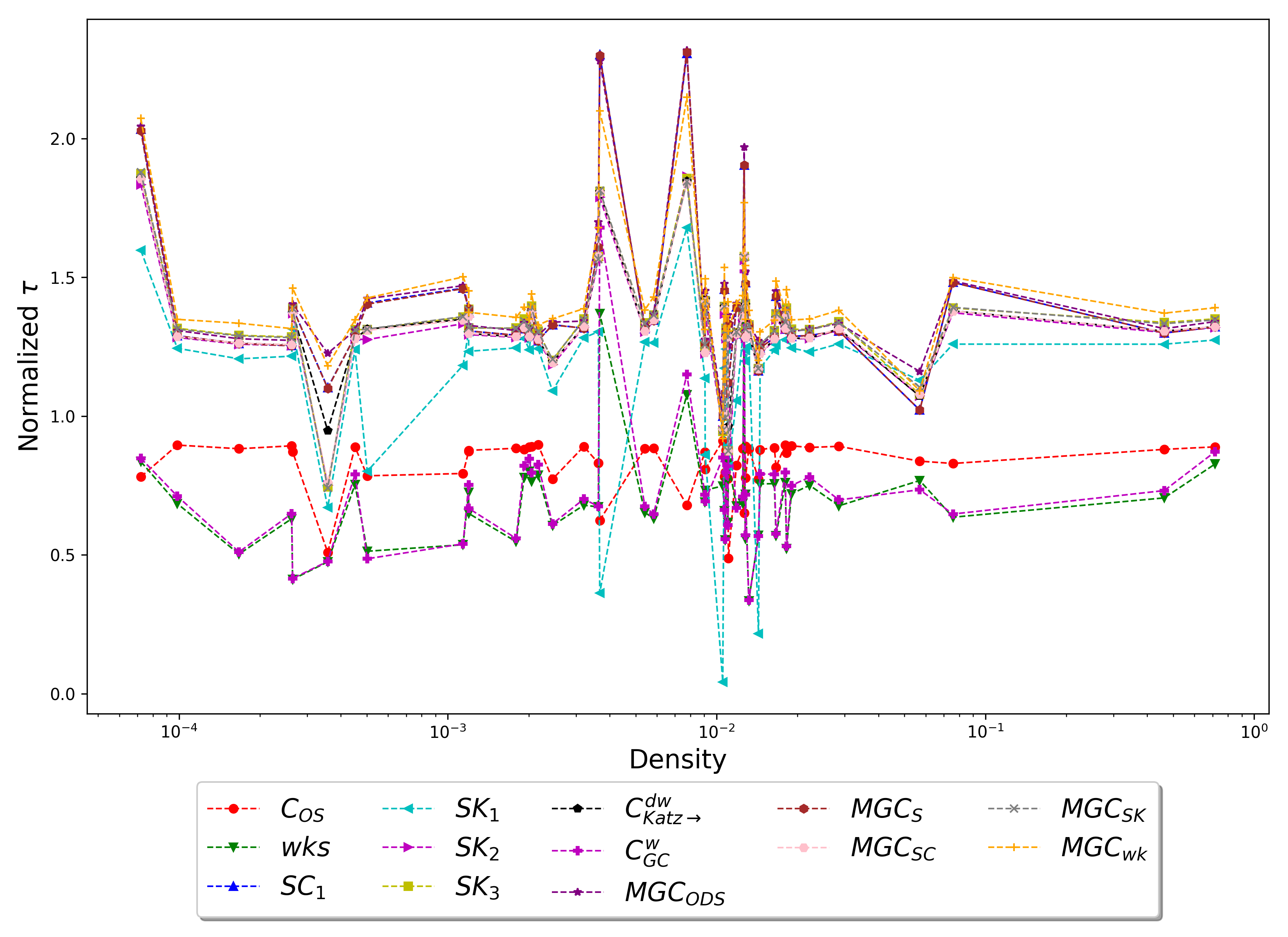
Figure 2: Graph density vs. normalized $\tau$ results of the measures.

Figure 3: Graph density vs. normalized $\epsilon$ results of the measures.

Finally, we inspect graph density vs. $\tau$ (Figure 2) and graph density vs. $\epsilon$ (Figure 3) to assess the stability of the centrality measures. In both figures, the $x$-axis corresponds to the graph density of the data sets, ordered from lowest to highest. The data show that the $\tau$ and $\epsilon$ values ($y$-axis) of the centrality measures do not change very much with graph density – but there are some peaks. Thus, the performance of the measures appears as reasonably stable w. r. t. this parameter.

Running Times

Running times of the proposed combined centrality measures as well as GC and its new variants were taken on a laptop with Intel Core i5 CPU at 1.6 GHz and 8 GB DDR3 RAM. Recall that all new measures as well as GC have been implemented in Python; basic centrality measures (uncombined) can be computed with NetworKit’s C++ backend.

In a nutshell, the results are: $C_{GC}^{w}$ and its variants fare very similar; also, $SK_{1}$’s running time is very close to the running time of $SK_{2}$ and $SK_{3}$. The combined centrality measures require a few seconds at most, often less. On average (arithmetic mean), $SC_{1}$ takes about one second, $C_{OS}$ and $SK_{1}$ only $3$ and $9$ thousandths, respectively. In contrast, the running time of GC and its variants can be quite high – even a few hours for the larger and denser graphs in our input collection and roughly $28$ minutes on average. These high running times for GC mostly stem from the iteration over $3$-hop neighborhoods. Thus, in this experimental setting, the combined measures are at least three orders of magnitude faster on average.

5 Conclusion

We have developed combined centrality measures with high prediction potential for the influence spread of nodes within the Independent Cascade (IC) model. These measures, including their extension of the state-of-the-art measure gravitational centrality (GC), show a significantly improved empirical performance compared to GC, both in correlation, monotonicity and in running time. Compared to related studies in the literature, we add a more meaningful perspective on the topic by using 50 public real-world data sets as weighted directed graphs in the common IC propagation model (as opposed to few unweighted/undirected graphs in the SIR model). Our new centrality combination with a closed formula takes care to use one local and one global centrality measure together. This approach unifies the local and global perspective of a node. Of course, there can be other ways to combine measures, e. g., by using multi-parameter regression.

How to assess the results in terms of the ranking performance measures, depends very much on the underlying algorithmic approach for IM. If we only pick the top-$k$ nodes as seeds, then the top-$k$ ranking results with lowest error $\epsilon$ are probably most useful (suggesting one of our GC variants). When applying metaheuristics to IM, Kendall $\tau$ results seems more useful as it allows a quick evaluation of new seed nodes. Ranking Monotonicity, on the other hand, is not necessarily useful when inspected in isolation. But a measure with low ranking monotonicity may be questionable.

Funding

This work was supported by The Scientific and Technological Research Council of Turkey (TÜBİTAK) [Project number: 1059B191700869]; and German Research Foundation (DFG) within Priority Programme 1736 [Grant: ME 3619/3-2].

Appendix A Input Data

Table 7: Data set properties

Data sets	$|V|$	$|E|$	Average outdegree	Density
Moreno seventh grader [43, 48]	29	376	12.97	0.4631
Moreno dutch college [43, 49]	32	710	22.19	0.7157
Moreno highschool [43, 50]	70	366	5.23	0.0758
Moreno residence hall [43, 51]	217	2672	12.31	0.0570
Moreno physicians [43, 52]	241	1098	4.56	0.0190
socfb-Haverford76 [44]	1446	59589	41.21	0.0285
socfb-Simmons81 [44]	1518	32988	21.73	0.0143
socfb-Swarthmore42 [44]	1659	61050	36.80	0.0222
Petster hamster friendships [43]	1858	12534	6.75	0.0036
Socfb-Amherst41 [44]	2235	90954	40.70	0.0182
socfb-Bowdoin47 [44]	2252	84387	37.47	0.0166
socfb-Hamilton46 [44]	2314	96394	41.66	0.0180
Moreno adolescent health [43, 53]	2539	12969	5.11	0.0020
socfb-Trinity100 [44]	2613	111996	42.86	0.0164
socfb-USFCA72 [44]	2682	65252	24.33	0.0091
socfb-Williams40 [44]	2790	112986	40.50	0.0145
socfb-nips-ego [44]	2888	2981	1.03	0.0004
socfb-Oberlin44 [44]	2920	89912	30.79	0.0105
socfb-Wellesley22 [44]	2970	94899	31.95	0.0108
socfb-Smith60 [44]	2970	97133	32.70	0.0110
socfb-Vassar85 [44]	3068	119161	38.84	0.0127
socfb-Middlebury45 [44]	3075	124610	40.52	0.0132
socfb-Pepperdine86 [44]	3445	152007	44.12	0.0128
socfb-Colgate88 [44]	3482	155043	44.53	0.0128
socfb-Santa74 [44]	3578	151747	42.41	0.0119
socfb-Wesleyan43 [44]	3593	138035	38.42	0.0107
socfb-Mich67 [44]	3748	81903	21.85	0.0058
socfb-Bucknell39 [44]	3826	158864	41.52	0.0109
Facebook 2018 tvshow [54]	3892	17262	4.44	0.0011
socfb-Brandeis99 [44]	3898	137567	35.29	0.0091
Facebook combined [55]	4039	88234	21.85	0.0054
socfb-Howard90 [44]	4047	204850	50.62	0.0125
socfb-Rice31 [44]	4087	184828	45.22	0.0111
socfb-Rochester38 [44]	4563	161404	35.37	0.0078
Facebook 2018 politician [54]	5908	41729	7.06	0.0012
Advogato [43, 56]	6539	51127	7.82	0.0012
Facebook 2018 government [54]	7057	89455	12.68	0.0018
Wiki-Vote [57, 58]	7115	103689	14.57	0.0020
socfb-BC17 [44]	11509	486967	42.31	0.0037
Facebook 2018 public figure [54]	11565	67114	5.80	0.0005
socfb-Columbia2 [44]	11770	444333	37.75	0.0032
Facebook 2018 athletes [54]	13866	86858	6.26	0.0005
socfb-JMU79 [44]	14070	485564	34.51	0.0025
Facebook 2018 company [54]	14113	52310	3.71	0.0003
socfb-UCSB37 [44]	14917	482215	32.33	0.0022
socfb-UCF52 [44]	14940	428989	28.71	0.0019
Facebook 2018 new sites [54]	27917	206259	7.39	0.0003
Deezer RO [54]	41773	125826	3.01	0.0001
Deezer HU [54]	47538	222887	4.69	0.0001
Deezer HR [54]	54573	498202	9.13	0.0002

Appendix B Performance Measures for Rankings

For completeness, we provide here the definitions for known measures for assessing the performance of rankings.

Definition 1 (Kendall $\tau$ ranking correlation [17, 59]).

Let $X$ and $Y$ be ranking lists, $n_{c}$ the number of concordant pairs, and $n_{d}$ the number of discordant pairs. Moreover, let $n_{0}:={\binom{n}{2}}$ and $n_{1}:=\sum_{i}t_{i}(t_{i}-1)/2$. Finally, let $n_{2}:=\sum_{j}t_{j}(t_{j}-1)/2$, where $t_{i}$ and $t_{j}$ are the number of tied values in the $i$th and $j$th group of ties in $X$ and $Y$, respectively. Then, the Kendall $\tau$ ranking correlation between $X$ and $Y$ is:

$$\tau(X,Y):={\frac{n_{c}-n_{d}}{\sqrt{(n_{0}-n_{1})\times(n_{0}-n_{2})}}}$$ (16)

Definition 2 (Ranking error [16]).

Let $f_{IC}(i)$ denote the expected spread of node $i$ in the IC model. Moreover, let $\phi(k)$ denote the set of top-$k$ nodes that are selected by a specific measure and let $\Phi(k)$ denote the set of top-$k$ nodes selected by expected spreads ranking of nodes within the IC model. Then, the ranking error $epsilon$ is given as:

$$\epsilon:=1-\frac{\sum_{i\in\phi(k)}f_{IC}(i)}{\sum_{j\in\Phi(k)}f_{IC}(i)}$$ (17)

Definition 3 (Ranking Monotonicity [16, 39]).

Let $R$ denote a ranking list and $|V|$ the number of nodes in the network. Moreover, let $|V|_{r}$ denote the number of nodes with rank $r$ in $R$. Then, the monotonicity of $R$, $M(R)$, is given as:

$$M(R):={\Bigg{(}1-\frac{\sum_{r\in V}|V|_{r}\times(|V|_{r}-1)}{|V|\times(|V|-1)}\Bigg{)}^{2}}$$ (18)

Appendix C Detailed Experimental Results

Table 8: Kendall $\tau$ results for basic measures normalized by $C_{OD}$

Data sets	$C_{OS}$	$C_{B}^{uu}$	$C_{B}^{uw}$	$C_{C}^{du}$	$\tilde{C}_{C}^{dw}$	$C_{E}^{uu}$	$C_{Katz}^{du}$	$wks$
Moreno seventh grader	1.07219	0.86828	0.0436	1.0895	1.05326	0.43518	0.04415	0.76777
Moreno dutch college	0.94924	0.48372	-0.12011	1	0.99014	0.75373	0.24781	0.74834
Moreno highschool	1.84211	0.59106	0.80837	1.30892	1.74549	-0.23471	-0.21467	1.07704
Moreno residence hall	1.16988	0.59655	-0.01666	0.87276	0.92799	0.41392	0.20729	0.56992
Moreno physicians	1.5771	0.52942	0.46768	0.40526	0.92737	-0.01444	0.05671	1.33096
socfb-Haverford76	1.28397	0.36361	-0.02064	0.38122	1.12532	0.30771	-0.32919	0.80109
socfb-Simmons81	1.22785	0.35745	0.04244	0.27842	0.91182	0.35444	-0.26511	0.68964
socfb-Swarthmore42	1.31375	0.399	-0.0258	0.34167	1.06816	0.31246	-0.31487	0.67667
Petster hamster friendships	1.85412	0.51868	0.51424	-0.36151	1.1611	0.30978	0.09258	0.83615
Socfb-Amherst41	1.28085	0.37866	-0.04531	0.46236	1.0534	0.30983	-0.29083	0.75061
socfb-Bowdoin47	1.28252	0.37619	0.009	0.45425	1.07021	0.29348	-0.31617	0.55806
socfb-Hamilton46	1.27881	0.34249	-0.01253	0.46144	1.11102	0.28117	-0.34063	0.75356
Moreno adolescent health	1.80561	0.56098	0.49428	1.37365	1.93651	0.08371	-0.14765	1.36908
socfb-Trinity100	1.27496	0.33278	-0.0074	0.48476	1.05317	0.29859	-0.31929	0.787
socfb-USFCA72	1.29699	0.41294	0.03016	0.45007	0.97061	0.36918	-0.17213	0.64924
socfb-Williams40	1.25598	0.35576	0.01324	0.52593	1.08511	0.31502	-0.28525	0.63013
socfb-nips-ego	0.91424	1.06276	0.84811	-0.03844	0.36752	0.46641	0.09795	0.83042
socfb-Oberlin44	1.35408	0.38774	0.02021	0.40455	1.04593	0.32949	-0.28713	0.68642
socfb-Smith60	1.22492	0.38594	0.01614	0.51633	1.00311	0.33518	-0.29024	0.75543
socfb-Wellesley22	1.37423	0.40136	-0.00929	0.34287	1.05348	0.32625	-0.28781	0.76453
socfb-Vassar85	1.31528	0.3276	-0.04416	0.46474	1.13225	0.28187	-0.35924	0.76019
socfb-Middlebury45	1.27759	0.37768	0.00691	0.35034	1.04371	0.32444	-0.26949	0.75653
socfb-Pepperdine86	1.30586	0.40344	0.03167	0.47996	1.03967	0.36903	-0.20436	0.7052
socfb-Colgate88	1.27992	0.30799	0.01587	0.42624	1.08471	0.26193	-0.36464	0.71967
socfb-Santa74	1.32182	0.36053	-0.04409	0.5468	1.10208	0.31662	-0.272	0.67879
socfb-Wesleyan43	1.32177	0.35419	-0.03332	0.48109	1.09294	0.30385	-0.31592	0.82727
socfb-Mich67	1.34677	0.44064	0.06052	0.43828	1.0198	0.36284	-0.18038	0.63085
socfb-Bucknell39	1.28519	0.32119	-0.03325	0.60848	1.0612	0.27474	-0.37136	0.6845
Facebook 2018 tvshow	1.41447	0.47297	0.35412	-0.54842	-0.11656	0.10791	-0.20833	0.73301
socfb-Brandeis99	1.26233	0.4091	-0.02065	0.60498	1.02234	0.3764	-0.1965	0.50282
Facebook combined	1.57412	0.3886	0.10442	-0.55989	0.23332	0.13391	-0.35056	0.6728
socfb-Howard90	1.31767	0.40883	-0.01443	0.58347	1.08569	0.38137	-0.20698	0.77934
socfb-Rice31	1.28138	0.37591	-0.0007	0.4965	1.07403	0.37021	-0.23798	0.75898
socfb-Rochester38	1.28599	0.34293	-0.01326	0.52499	1.0627	0.31673	-0.25947	0.54769
Facebook 2018 politician	1.39533	0.48556	0.2948	-0.70569	0.00676	0.17049	-0.19246	0.7189
advogato	0.76081	0.7351	0.43044	0.85957	0.91846	0.6862	0.60825	0.47472
Facebook 2018 government	1.35247	0.43016	0.15733	-0.22203	0.53554	0.18745	-0.16143	0.56916
Wiki-Vote	1.00791	0.66257	0.44556	0.59118	0.60544	0.77417	0.46799	0.55412
Socfb-BC17	1.3052	0.37091	-0.03239	0.68327	1.08855	0.37081	-0.23247	0.65282
Facebook 2018 public figure	1.38879	0.57016	0.34058	-0.35101	0.18357	0.22931	-0.01495	0.65866
socfb-Columbia2	1.36419	0.45096	0.02765	0.7161	1.09404	0.41569	-0.12648	0.52236
Facebook 2018 athletes	1.1923	0.48305	0.27088	-0.31938	0.2857	0.3161	-0.09231	0.60546
socfb-JMU79	1.29742	0.36219	-0.04413	0.78601	1.07609	0.37797	-0.27027	0.33486
Facebook 2018 company	1.28638	0.47791	0.34551	-0.57644	-0.20005	0.20814	-0.12015	0.61745
socfb-UCSB37	1.35853	0.41187	-0.01882	0.71768	1.10934	0.39657	-0.17722	0.72479
socfb-UCF52	1.37173	0.43188	0.00187	0.67341	0.98016	0.41325	-0.14063	0.41168
Facebook 2018 new sites	1.34588	0.4677	0.20821	-0.19962	0.33479	0.28954	-0.1521	0.53644
Deezer RO	1.30968	0.39828	0.17782	-0.79879	-0.47604	0.2095	-0.28423	0.513
Deezer HU	1.29675	0.35853	0.0919	-0.78482	-0.34168	0.26132	-0.34625	0.67605
Deezer HR	1.37833	0.40432	0.06735	-0.1702	0.51123	0.36759	-0.22419	0.63562
geometric mean	1.29864	0.43427	0.051259	0.491424	0.725396	0.291757	0.208434	0.67953

Table 9: Normalized Kendall $\tau$ results for combined measures

Data sets	$SC_{1}$	$SK_{1}$	$SK_{2}$	$SK_{3}$	$C_{Katz\rightarrow}^{dw}$
Moreno seventh grader	1.02173	1.12895	1.07219	1.07849	1.07219
Moreno dutch college	0.99964	0.042	0.94924	0.94504	0.94924
Moreno highschool	2.3055	1.67887	1.86304	1.8563	1.84658
Moreno residence hall	1.16266	0.21573	1.16537	1.17091	1.16988
Moreno physicians	1.90406	1.29563	1.5627	1.57417	1.57725
socfb-Haverford76	1.29127	1.23903	1.28214	1.31473	1.28412
socfb-Simmons81	1.26075	1.13576	1.22459	1.25217	1.22797
socfb-Swarthmore42	1.30656	1.26022	1.31087	1.34036	1.31386
Petster hamster friendships	2.03253	1.59719	1.83377	1.87295	1.85556
Socfb-Amherst41	1.29013	1.23109	1.27887	1.31191	1.28096
socfb-Bowdoin47	1.2893	1.23733	1.28024	1.31379	1.28264
socfb-Hamilton46	1.28768	1.2393	1.27684	1.31151	1.27891
Moreno adolescent health	2.30235	0.36232	1.78791	1.80946	1.80672
socfb-Trinity100	1.27118	1.24274	1.27346	1.30606	1.27505
socfb-USFCA72	1.3065	1.23325	1.29336	1.31714	1.29715
socfb-Williams40	1.25352	1.21565	1.25386	1.28535	1.25609
socfb-nips-ego	1.12072	0.81988	0.81988	0.87383	0.96288
socfb-Oberlin44	1.36136	1.28213	1.35199	1.38201	1.35422
socfb-Smith60	1.24548	1.17268	1.22259	1.25609	1.22502
socfb-Wellesley22	1.36897	1.32054	1.37127	1.39548	1.37435
socfb-Vassar85	1.31344	1.2748	1.31266	1.34281	1.31538
socfb-Middlebury45	1.2818	1.23765	1.27519	1.30794	1.27773
socfb-Pepperdine86	1.29885	1.25882	1.3012	1.33746	1.306
socfb-Colgate88	1.28686	1.24514	1.27882	1.31266	1.28003
socfb-Santa74	1.31672	1.28173	1.31999	1.35012	1.32193
socfb-Wesleyan43	1.32115	1.27399	1.31886	1.34998	1.32191
socfb-Mich67	1.34482	1.26409	1.34299	1.36394	1.34692
socfb-Bucknell39	1.28908	1.24405	1.28313	1.31614	1.2853
Facebook 2018 tvshow	1.40682	0.8598	1.36151	1.41537	1.42149
socfb-Brandeis99	1.26142	1.20605	1.25883	1.29074	1.26246
Facebook combined	1.60939	1.30368	1.56052	1.57443	1.57445
socfb-Howard90	1.31449	1.27997	1.31616	1.34902	1.3178
socfb-Rice31	1.28918	1.2417	1.27935	1.31631	1.2815
socfb-Rochester38	1.29122	1.24549	1.28376	1.31682	1.2861
Facebook 2018 politician	1.48084	1.19778	1.37895	1.40473	1.40002
advogato	1.10156	0.67022	0.75117	0.74454	0.94766
Facebook 2018 government	1.43131	1.25692	1.34626	1.3686	1.35283
Wiki-Vote	1.08119	0.99839	1.00578	0.99949	1.00823
Socfb-BC17	1.31419	1.26612	1.30292	1.33626	1.30531
Facebook 2018 public figure	1.45592	1.1719	1.36848	1.39434	1.39342
socfb-Columbia2	1.37154	1.30789	1.35883	1.38909	1.36435
Facebook 2018 athletes	1.32884	1.09071	1.18449	1.20103	1.19443
socfb-JMU79	1.3225	1.25209	1.29578	1.32809	1.29754
Facebook 2018 company	1.33801	0.8942	1.24648	1.28932	1.29482
socfb-UCSB37	1.38757	1.30484	1.35613	1.3848	1.35867
socfb-UCF52	1.38952	1.31247	1.36919	1.389	1.37189
Facebook 2018 new sites	1.46062	1.1829	1.33249	1.35655	1.34878
Deezer RO	1.40734	0.80106	1.27555	1.31152	1.31279
Deezer HU	1.39269	1.05544	1.28433	1.30042	1.29783
Deezer HR	1.48176	1.25906	1.37196	1.38919	1.37875
geometric mean	1.35576	1.04994	1.28907	1.31493	1.30657

Table 10: Normalized Kendall $\tau$ results for modifications of gravitational centrality

Data sets	$C_{GC}^{w}$	$MGC_{ODS}$	$MGC_{S}$	$MGC_{SC}$	$MGC_{SK}$	$MGC_{wk}$
Moreno seventh grader	0.73459	1.16048	1.02173	1.07849	1.10372	1.09111
Moreno dutch college	0.85002	1.00804	0.99964	0.95344	0.94924	0.91984
Moreno highschool	1.1495	2.31673	2.30999	1.83834	1.84507	2.14828
Moreno residence hall	0.56771	1.27052	1.16317	1.17027	1.17066	1.20033
Moreno physicians	1.52192	1.96817	1.90406	1.57725	1.57131	1.76854
socfb-Haverford76	0.84677	1.3151	1.2913	1.28578	1.31109	1.34965
socfb-Simmons81	0.71641	1.27526	1.26071	1.22916	1.25748	1.31159
socfb-Swarthmore42	0.69794	1.33336	1.30655	1.31462	1.33739	1.38106
Petster hamster friendships	0.84828	2.04285	2.02824	1.85425	1.87918	2.07271
Socfb-Amherst41	0.77978	1.31293	1.29016	1.28161	1.30967	1.34943
socfb-Bowdoin47	0.57039	1.30414	1.28926	1.28366	1.31301	1.3482
socfb-Hamilton46	0.78984	1.30853	1.28771	1.27967	1.30965	1.34618
Moreno adolescent health	1.6793	2.27963	2.29936	1.80534	1.81307	2.09881
socfb-Trinity100	0.82539	1.29106	1.27117	1.27605	1.30344	1.32765
socfb-USFCA72	0.66755	1.32653	1.30637	1.29776	1.31831	1.37363
socfb-Williams40	0.64841	1.27252	1.25352	1.25718	1.28258	1.31505
socfb-nips-ego	1.01414	1.25598	1.12072	0.87383	0.87383	1.30608
socfb-Oberlin44	0.70955	1.37339	1.36131	1.35471	1.38163	1.4336
socfb-Smith60	0.79162	1.25405	1.24552	1.22554	1.25862	1.30391
socfb-Wellesley22	0.79596	1.38155	1.36873	1.37451	1.39211	1.44012
socfb-Vassar85	0.79713	1.33655	1.31337	1.31608	1.33868	1.38237
socfb-Middlebury45	0.79021	1.29392	1.28173	1.27855	1.30642	1.345
socfb-Pepperdine86	0.7316	1.31475	1.29875	1.30663	1.33287	1.37074
socfb-Colgate88	0.74988	1.30449	1.28689	1.28092	1.30904	1.34626
socfb-Santa74	0.70084	1.34198	1.31664	1.32237	1.34499	1.38677
socfb-Wesleyan43	0.87143	1.34025	1.32113	1.32203	1.34634	1.39005
socfb-Mich67	0.64648	1.36589	1.34467	1.34715	1.36307	1.42902
socfb-Bucknell39	0.7113	1.3081	1.28901	1.28633	1.31292	1.34831
Facebook 2018 tvshow	0.69339	1.45027	1.40002	1.41356	1.41549	1.49404
socfb-Brandeis99	0.51041	1.2783	1.26135	1.26236	1.28888	1.33432
Facebook combined	0.67483	1.69784	1.60843	1.57409	1.56488	1.67843
socfb-Howard90	0.82153	1.33585	1.31452	1.31836	1.3412	1.39143
socfb-Rice31	0.79711	1.31074	1.28919	1.28239	1.3122	1.36068
socfb-Rochester38	0.55915	1.30834	1.29121	1.28625	1.31587	1.35564
Facebook 2018 politician	0.71679	1.52019	1.47809	1.39526	1.40782	1.54248
advogato	0.47654	1.22577	1.09978	0.76072	0.74031	1.18128
Facebook 2018 government	0.57675	1.44967	1.43062	1.3525	1.37007	1.48547
Wiki-Vote	0.55593	1.08693	1.08121	1.00789	0.9945	1.13243
Socfb-BC17	0.67427	1.32557	1.31418	1.30554	1.33301	1.38271
Facebook 2018 public figure	0.66155	1.47636	1.45225	1.38843	1.39538	1.53463
socfb-Columbia2	0.53067	1.37866	1.3713	1.36421	1.38497	1.45478
Facebook 2018 athletes	0.61181	1.33842	1.32811	1.19227	1.20419	1.35043
socfb-JMU79	0.33717	1.3333	1.32253	1.29744	1.32671	1.38115
Facebook 2018 company	0.60783	1.3633	1.33336	1.28576	1.29077	1.41088
socfb-UCSB37	0.75196	1.39101	1.38756	1.35906	1.38202	1.45049
socfb-UCF52	0.41494	1.4033	1.38954	1.37175	1.3872	1.46115
Facebook 2018 new sites	0.53968	1.46971	1.45859	1.3458	1.35829	1.50102
Deezer RO	0.48595	1.42253	1.40325	1.30878	1.31349	1.42544
Deezer HU	0.66951	1.40481	1.39164	1.29645	1.30283	1.40613
Deezer HR	0.64705	1.48671	1.48101	1.37828	1.39161	1.49918
geometric mean	0.70205	1.38455	1.35513	1.29802	1.31421	1.40721

Table 11: Normalized $\epsilon$ for $C_{OS}$, $wks$, $C_{Katz\rightarrow}^{dw}$, and the proposed combined measures

Data sets	$C_{OS}$	$wks$	$SC_{1}$	$SK_{1}$	$SK_{2}$	$SK_{3}$	$C_{Katz\rightarrow}^{dw}$
Moreno residence hall	0.25512	0.69927	0.29313	0.31851	0.33243	0.33487	0.25512
Moreno physicians	0.30256	0.37274	0.30256	0.30256	0.30256	0.30256	0.30256
socfb-Haverford76	0.26202	0.47165	0.26202	0.22385	0.22062	0.21282	0.26202
socfb-Simmons81	0.54007	0.71912	0.54007	0.48921	0.49367	0.48965	0.54007
socfb-Swarthmore42	0.46276	0.6336	0.46276	0.35905	0.45217	0.35905	0.46276
Petster hamster friendships	0.39754	0.61945	0.39754	0.35454	0.36399	0.3498	0.39754
Socfb-Amherst41	0.36125	0.68422	0.36125	0.31794	0.34848	0.28005	0.36125
socfb-Bowdoin47	0.30648	0.50406	0.30648	0.25929	0.25929	0.24939	0.30648
socfb-Hamilton46	0.37336	0.78778	0.37336	0.25364	0.30259	0.25686	0.37336
Moreno adolescent health	0.42094	0.47341	0.42094	0.42358	0.42094	0.4113	0.42094
socfb-Trinity100	0.46712	0.65428	0.46712	0.36999	0.38724	0.35247	0.46712
socfb-USFCA72	0.38633	0.84379	0.38633	0.3566	0.36694	0.35349	0.38633
socfb-Williams40	0.49189	0.78705	0.49189	0.41761	0.41761	0.41284	0.49189
socfb-nips-ego	1	1	1	1	1	1	1
socfb-Oberlin44	0.3785	0.47519	0.3785	0.31897	0.35904	0.31644	0.3785
socfb-Smith60	0.24135	0.41943	0.24135	0.2032	0.2032	0.2032	0.24135
socfb-Wellesley22	0.48079	0.76193	0.48079	0.44613	0.46375	0.41113	0.48079
socfb-Vassar85	0.25668	0.62991	0.25668	0.25211	0.25211	0.21918	0.25668
socfb-Middlebury45	0.46514	0.57362	0.46514	0.38526	0.38526	0.31756	0.46514
socfb-Pepperdine86	0.3885	0.75458	0.3885	0.3325	0.35018	0.31855	0.3885
socfb-Colgate88	0.51404	0.72975	0.51404	0.47323	0.49853	0.45644	0.51404
socfb-Santa74	0.32979	0.59999	0.32979	0.27099	0.30347	0.24535	0.32979
socfb-Wesleyan43	0.29342	0.58256	0.29342	0.25977	0.25977	0.26154	0.29342
socfb-Mich67	0.67358	0.83665	0.67358	0.51844	0.52565	0.48376	0.67358
socfb-Bucknell39	0.41871	0.59615	0.41871	0.38348	0.39553	0.35257	0.41871
Facebook 2018 tvshow	0.61928	0.59371	0.56083	0.56107	0.56107	0.56752	0.61239
socfb-Brandeis99	0.32414	0.53625	0.32414	0.26547	0.26547	0.24321	0.32414
Facebook combined	0.55791	0.66992	0.56234	0.53208	0.53208	0.51662	0.55791
socfb-Howard90	0.40548	0.71537	0.40548	0.27983	0.33532	0.26495	0.40548
socfb-Rice31	0.44395	0.57937	0.44395	0.39381	0.39684	0.39381	0.44395
socfb-Rochester38	0.27909	0.60616	0.27909	0.23	0.23492	0.22546	0.27909
Facebook 2018 politician	0.53271	0.67737	0.53271	0.50283	0.50283	0.51869	0.53271
advogato	1.04794	0.73164	1.04794	0.98956	0.95241	0.98956	1.03962
Facebook 2018 government	0.48642	0.65609	0.48642	0.4455	0.4455	0.4455	0.48642
Wiki-Vote	0.47074	0.44612	0.47074	0.53308	0.56687	0.68054	0.47074
Socfb-BC17	0.57718	0.70532	0.57718	0.47559	0.56096	0.47666	0.57718
Facebook 2018 public figure	0.66701	0.66535	0.66701	0.62448	0.63913	0.62449	0.67371
socfb-Columbia2	0.66694	0.81704	0.66694	0.56962	0.56962	0.56962	0.66694
Facebook 2018 athletes	0.92226	0.88353	0.92226	0.83905	0.8565	0.82413	0.92226
socfb-JMU79	0.53781	0.81163	0.53781	0.43576	0.43576	0.43385	0.53781
Facebook 2018 company	0.76854	0.70986	0.75373	0.72783	0.72783	0.72783	0.76854
socfb-UCSB37	0.66844	0.73694	0.66844	0.62428	0.65571	0.61348	0.66844
socfb-UCF52	0.52686	0.72915	0.52686	0.50551	0.52086	0.49955	0.52686
Facebook 2018 new sites	0.70388	0.71843	0.70388	0.65429	0.67445	0.65429	0.70388
Deezer RO	0.73214	0.82637	0.73214	0.73214	0.73214	0.70391	0.73214
Deezer HU	0.6953	0.70415	0.6953	0.68203	0.68695	0.67093	0.6953
Deezer HR	0.75138	0.81517	0.75138	0.69428	0.72058	0.69603	0.75138
geometric mean	0.47425	0.65788	0.47453	0.42411	0.43921	0.41501	0.47415

Table 12: Normalized $\epsilon$ for modifications of gravitational centrality.

Data sets	$C_{GC}^{w}$	$MGC_{ODS}$	$MGC_{S}$	$MGC_{SC}$	$MGC_{SK}$	$MGC_{wk}$
Moreno residence hall	2.448	0.11315	0.42324	0.42324	0.51414	0.38118
Moreno physicians	0.20283	0.10236	0.21894	0.21894	0.18107	0.2643
socfb-Haverford76	0.11135	0.01677	0.01707	0.01707	0.02279	0.08911
socfb-Simmons81	0.32375	0.0525	0.05035	0.05035	0.05267	0.22209
socfb-Swarthmore42	0.09462	0.02152	0.04461	0.04461	0.0505	0.09746
Petster hamster friendships	0.43121	0.11701	0.15453	0.14662	0.18088	0.32448
Socfb-Amherst41	0.06586	0.02541	0.02802	0.02802	0.02802	0.09175
socfb-Bowdoin47	0.20356	0.01704	0.02473	0.02473	0.03083	0.08075
socfb-Hamilton46	0.06337	0.03676	0.03763	0.03763	0.04067	0.13756
Moreno adolescent health	0.26861	0.18761	0.13217	0.13217	0.13217	0.3275
socfb-Trinity100	0.08626	0.04673	0.04301	0.04301	0.04422	0.15279
socfb-USFCA72	0.14782	0.05549	0.08039	0.08039	0.08039	0.23444
socfb-Williams40	0.18012	0.04529	0.05901	0.05901	0.05901	0.19405
socfb-nips-ego	1	1	1	1	1	1
socfb-Oberlin44	0.10535	0.10038	0.06695	0.06695	0.05149	0.12517
socfb-Smith60	0.1146	0.03551	0.0295	0.0295	0.03189	0.16791
socfb-Wellesley22	0.17402	0.01778	0.05613	0.05613	0.05921	0.22957
socfb-Vassar85	0.03984	0.02785	0.03876	0.03876	0.03876	0.07046
socfb-Middlebury45	0.10623	0.03542	0.02143	0.02143	0.02863	0.18416
socfb-Pepperdine86	0.10288	0.03321	0.03023	0.03023	0.02289	0.11396
socfb-Colgate88	0.23763	0.07742	0.03966	0.03966	0.03966	0.29269
socfb-Santa74	0.08188	0.04581	0.03994	0.03994	0.03751	0.12454
socfb-Wesleyan43	0.09717	0.0468	0.03625	0.03625	0.03142	0.13584
socfb-Mich67	0.08518	0.09433	0.10884	0.10884	0.10278	0.29759
socfb-Bucknell39	0.19714	0.04229	0.04841	0.04841	0.04841	0.18054
Facebook 2018 tvshow	0.18434	0.17221	0.24594	0.26484	0.26063	0.42753
socfb-Brandeis99	0.17139	0.0196	0.01558	0.01558	0.01558	0.11424
Facebook combined	0.49939	0.19561	0.12713	0.12713	0.12713	0.16093
socfb-Howard90	0.0792	0.05839	0.06017	0.06017	0.04334	0.11557
socfb-Rice31	0.072	0.0766	0.06589	0.06589	0.06419	0.14502
socfb-Rochester38	0.10521	0.03811	0.04021	0.04021	0.03391	0.1071
Facebook 2018 politician	0.15745	0.09422	0.19236	0.19236	0.20892	0.44732
advogato	0.27719	0.33991	0.56697	0.56697	0.59685	0.8474
Facebook 2018 government	0.13169	0.13371	0.18233	0.18233	0.15915	0.31694
Wiki-Vote	0.10855	0.49188	0.65787	0.65787	1.32246	1.58915
Socfb-BC17	0.08558	0.06673	0.07063	0.07063	0.04905	0.21086
Facebook 2018 public figure	0.21784	0.17261	0.31177	0.2801	0.231	0.54453
socfb-Columbia2	0.16332	0.12478	0.10754	0.10754	0.10754	0.26202
Facebook 2018 athletes	0.22149	0.31631	0.22155	0.22155	0.17837	0.70301
socfb-JMU79	0.28261	0.15332	0.13874	0.13874	0.13874	0.27724
Facebook 2018 company	0.2098	0.29788	0.22984	0.22079	0.21741	0.62358
socfb-UCSB37	0.14998	0.09283	0.06006	0.06006	0.05773	0.19566
socfb-UCF52	0.13389	0.13706	0.16518	0.16518	0.12535	0.3586
Facebook 2018 new sites	0.31945	0.23881	0.23164	0.23164	0.20128	0.53716
Deezer RO	0.30249	0.26882	0.27234	0.27234	0.25782	0.51047
Deezer HU	0.20487	0.19902	0.21211	0.21211	0.21211	0.45621
Deezer HR	0.26697	0.33505	0.26885	0.26885	0.26257	0.53277
geometric mean	0.16681	0.08432	0.09198	0.09174	0.09066	0.24280

Table 13: Ranking Monotonicity values for $C_{OS}$, $wks$, $C_{Katz\rightarrow}^{dw}$, and the proposed combined measures

Data sets	$C_{OS}$	$wks$	$SC_{1}$	$SK_{1}$	$SK_{2}$	$SK_{3}$	$C_{Katz\rightarrow}^{dw}$
Moreno seventh grader	1	0.0398	1	1	1	1	1
Moreno dutch college	1	0.01513	1	1	1	1	1
Moreno highschool	0.99504	0.00714	1	1	1	1	1
Moreno residence hall	1	0.00208	1	1	1	1	1
Moreno physicians	0.99806	0.04491	1	1	1	1	1
socfb-Haverford76	0.99989	0.01022	0.99993	1	1	1	0.99993
socfb-Simmons81	0.99944	0.02382	0.9999	0.99998	0.99998	0.99998	0.9999
socfb-Swarthmore42	0.99985	0.01822	0.99997	1	1	1	0.99997
Petster hamster friendships	0.84912	0.02653	0.91699	0.9191	0.91994	0.91994	0.91699
Socfb-Amherst41	0.99981	0.01556	0.99995	1	1	1	0.99995
socfb-Bowdoin47	0.9998	0.01767	0.99998	1	1	1	0.99998
socfb-Hamilton46	0.99989	0.0134	0.99997	1	1	1	0.99997
Moreno adolescent health	0.91861	0.03401	0.99995	0.99995	0.99995	0.99995	0.99998
socfb-Trinity100	0.99991	0.01714	0.99999	1	1	1	0.99999
socfb-USFCA72	0.99824	0.03555	0.99986	0.99998	0.99998	0.99998	0.99986
socfb-Williams40	0.99981	0.01731	0.99997	1	1	1	0.99997
socfb-nips-ego	0.99997	0.99993	0.99998	0.99999	0.99999	0.99999	0.99998
socfb-Oberlin44	0.99943	0.02982	0.99994	0.99999	0.99999	0.99999	0.99994
socfb-Smith60	0.99944	0.02601	0.99984	1	1	1	0.99984
socfb-Wellesley22	0.99953	0.02742	0.99993	1	1	1	0.99993
socfb-Vassar85	0.99985	0.01426	0.99996	1	1	1	0.99997
socfb-Middlebury45	0.99946	0.02197	0.99995	1	1	1	0.99995
socfb-Pepperdine86	0.99932	0.02937	0.99985	0.99995	0.99995	0.99995	0.99986
socfb-Colgate88	0.99985	0.0142	0.99999	1	1	1	0.99999
socfb-Santa74	0.99973	0.0202	0.9999	0.99999	0.99999	0.99999	0.9999
socfb-Wesleyan43	0.99966	0.02337	0.99996	1	1	1	0.99996
socfb-Mich67	0.99711	0.04927	0.99971	0.99994	0.99994	0.99994	0.99971
socfb-Bucknell39	0.99986	0.01962	0.99997	1	1	1	0.99997
Facebook 2018 tvshow	0.82555	0.24428	0.96548	0.96886	0.96911	0.96911	0.96936
socfb-Brandeis99	0.99935	0.03458	0.99991	0.99998	0.99998	0.99998	0.99991
Facebook combined	0.99051	0.06099	0.99831	0.99998	0.99998	0.99998	0.99845
socfb-Howard90	0.99954	0.0265	0.99995	1	1	1	0.99995
socfb-Rice31	0.99966	0.02558	0.99994	1	1	1	0.99994
socfb-Rochester38	0.99954	0.03071	0.99994	1	1	1	0.99994
Facebook 2018 politician	0.9271	0.17586	0.9884	0.99181	0.99185	0.99185	0.98835
advogato	0.98435	0.43515	0.99883	0.99825	0.99825	0.99825	0.99661
Facebook 2018 government	0.97943	0.11658	0.9968	0.99895	0.99895	0.99895	0.99686
Wiki-Vote	0.9655	0.40037	0.98887	0.96793	0.96793	0.96793	0.98887
Socfb-BC17	0.9994	0.07503	0.99998	0.99998	0.99998	0.99998	0.99998
Facebook 2018 public figure	0.89544	0.29705	0.98941	0.9802	0.9803	0.9802	0.99001
socfb-Columbia2	0.99774	0.11542	0.99983	0.99977	0.99977	0.99977	0.99983
Facebook 2018 athletes	0.94458	0.24277	0.99424	0.99567	0.9957	0.9957	0.99421
socfb-JMU79	0.9993	0.08415	0.99998	0.99999	0.99999	0.99999	0.99998
Facebook 2018 company	0.82812	0.32434	0.97689	0.96469	0.96491	0.96499	0.97941
socfb-UCSB37	0.99859	0.11029	0.99996	0.99994	0.99994	0.99994	0.99996
socfb-UCF52	0.99739	0.11593	0.99989	0.99995	0.99995	0.99995	0.99989
Facebook 2018 new sites	0.94966	0.31787	0.99659	0.99441	0.9944	0.99441	0.99685
Deezer RO	0.77783	0.46095	0.99208	0.95579	0.95586	0.9559	0.9949
Deezer HU	0.87108	0.39118	0.99695	0.98997	0.99008	0.99004	0.99765
Deezer HR	0.9742	0.38287	0.99946	0.99833	0.99835	0.99834	0.99949
geometric mean	0.97148	0.05049	0.99585	0.99435	0.99438	0.99438	0.99603

Table 14: Ranking Monotonicity values for modifications of gravitational centrality.

Data sets	$C_{GC}^{w}$	$MGC_{ODS}$	$MGC_{S}$	$MGC_{SC}$	$MGC_{SK}$	$MGC_{wk}$
Moreno seventh grader	0.18579	1	1	1	1	1
Moreno dutch college	0.47822	1	1	1	1	1
Moreno highschool	0.08498	1	1	1	1	1
Moreno residence hall	0.02816	1	1	1	1	1
Moreno physicians	0.73685	0.99993	0.99993	0.99993	1	1
socfb-Haverford76	0.23123	0.99956	0.99956	0.99956	0.99977	0.99993
socfb-Simmons81	0.17236	0.99903	0.99903	0.99903	0.99908	0.9999
socfb-Swarthmore42	0.12773	0.99953	0.99953	0.99953	0.99956	0.99997
Petster hamster friendships	0.11237	0.91399	0.91356	0.91442	0.94663	0.91741
Socfb-Amherst41	0.18578	0.99965	0.99965	0.99965	0.99986	0.99995
socfb-Bowdoin47	0.08701	0.99968	0.99968	0.99968	0.99978	0.99998
socfb-Hamilton46	0.18893	0.99976	0.99976	0.99976	0.99989	0.99997
Moreno adolescent health	0.75033	0.99994	0.99994	0.99994	0.99994	1
socfb-Trinity100	0.23114	0.99988	0.99988	0.99988	0.99993	0.99999
socfb-USFCA72	0.14526	0.99926	0.99926	0.99926	0.9995	0.99986
socfb-Williams40	0.11667	0.99985	0.99985	0.99985	0.99991	0.99997
socfb-nips-ego	0.99989	0.99996	0.99996	0.99996	0.99997	0.99998
socfb-Oberlin44	0.15114	0.99958	0.99958	0.99958	0.99963	0.99994
socfb-Smith60	0.23876	0.99928	0.99928	0.99928	0.99957	0.99984
socfb-Wellesley22	0.18772	0.99947	0.99947	0.99947	0.99957	0.99993
socfb-Vassar85	0.1906	0.99979	0.99979	0.99979	0.99987	0.99997
socfb-Middlebury45	0.20712	0.99973	0.99973	0.99973	0.99985	0.99995
socfb-Pepperdine86	0.17224	0.99952	0.99952	0.99952	0.99976	0.99986
socfb-Colgate88	0.16582	0.9998	0.9998	0.9998	0.99986	0.99999
socfb-Santa74	0.1379	0.99968	0.99968	0.99968	0.99985	0.9999
socfb-Wesleyan43	0.26978	0.99973	0.99973	0.99973	0.99984	0.99996
socfb-Mich67	0.14673	0.99873	0.99873	0.99873	0.99933	0.99971
socfb-Bucknell39	0.15732	0.99981	0.99981	0.99981	0.99987	0.99997
Facebook 2018 tvshow	0.36418	0.96179	0.96123	0.96304	0.97882	0.97219
socfb-Brandeis99	0.09087	0.99956	0.99956	0.99956	0.99974	0.99991
Facebook combined	0.14512	0.99672	0.99672	0.99672	0.99785	0.99848
socfb-Howard90	0.21934	0.9997	0.9997	0.9997	0.99981	0.99995
socfb-Rice31	0.21706	0.99964	0.99964	0.99964	0.99979	0.99994
socfb-Rochester38	0.10144	0.99974	0.99974	0.99974	0.99987	0.99994
Facebook 2018 politician	0.28619	0.98412	0.9843	0.98447	0.99379	0.98926
advogato	0.48197	0.99913	0.99913	0.99917	0.99945	0.99952
Facebook 2018 government	0.18878	0.99482	0.99482	0.99482	0.9976	0.99693
Wiki-Vote	0.49329	0.98226	0.98226	0.98226	0.98252	0.98928
Socfb-BC17	0.21013	0.99991	0.99991	0.99991	0.99995	0.99998
Facebook 2018 public figure	0.39146	0.98715	0.98696	0.9874	0.99447	0.99072
socfb-Columbia2	0.18284	0.99967	0.99967	0.99967	0.99979	0.99983
Facebook 2018 athletes	0.346	0.9918	0.99173	0.99186	0.99642	0.9945
socfb-JMU79	0.11089	0.9999	0.9999	0.9999	0.99994	0.99998
Facebook 2018 company	0.4071	0.9757	0.97492	0.97652	0.98878	0.98193
socfb-UCSB37	0.27912	0.99987	0.99987	0.99987	0.99993	0.99996
socfb-UCF52	0.15485	0.99969	0.99969	0.99969	0.99983	0.99989
Facebook 2018 new sites	0.37889	0.99599	0.99589	0.99612	0.99836	0.99729
Deezer RO	0.50332	0.99347	0.99286	0.99403	0.99781	0.99563
Deezer HU	0.49947	0.9968	0.99666	0.9969	0.99836	0.99786
Deezer HR	0.4801	0.99913	0.99911	0.99914	0.99943	0.99951
geometric mean	0.21740	0.99513	0.99508	0.99521	0.99722	0.99628

References

- Henri and Pudelko [2003] F. Henri and B. Pudelko. Understanding and analysing activity and learning in virtual communities. Journal of Computer Assisted Learning, 19(4):474–487, dec 2003. ISSN 02664909.
- Zareie and Sheikhahmadi [2018] Ahmad Zareie and Amir Sheikhahmadi. A hierarchical approach for influential node ranking in complex social networks. Expert Systems With Applications, 93:200–211, 2018. ISSN 0957-4174.
- Kimura et al. [2010] Masahiro Kimura, Kazumi Saito, Ryohei Nakano, and Hiroshi Motoda. Extracting influential nodes on a social network for information diffusion. Data Mining and Knowledge Discovery, 20(1):70–97, jan 2010. ISSN 1384-5810.
- Sheikhahmadi et al. [2017] Amir Sheikhahmadi, Mohammad Ali Nematbakhsh, and Ahmad Zareie. Identification of influential users by neighbors in online social networks. Physica A: Statistical Mechanics and its Applications, 486:517–534, nov 2017. ISSN 03784371.
- Chevalier and Mayzlin [2006] Judith A. Chevalier and Dina Mayzlin. The Effect of Word of Mouth on Sales: Online Book Reviews. Journal of Marketing Research, 43(3):345–354, aug 2006. ISSN 0022-2437.
- Probst et al. [2013] Florian Probst, Laura Grosswiele, and Regina Pfleger. Who will lead and who will follow: Identifying Influential Users in Online Social Networks. Business & Information Systems Engineering, 5(3):179–193, jun 2013. ISSN 1867-0202.
- Madar et al. [2004] N. Madar, T. Kalisky, R. Cohen, D. Ben-Avraham, and S. Havlin. Immunization and epidemic dynamics in complex networks. The European Physical Journal B - Condensed Matter, 38(2):269–276, mar 2004. ISSN 1434-6028.
- Pastor-Satorras and Vespignani [2001] Romualdo Pastor-Satorras and Alessandro Vespignani. Epidemic Spreading in Scale-Free Networks. Physical Review Letters, 86(14):3200–3203, apr 2001. ISSN 0031-9007.
- Li et al. [2018] Yuchen Li, Ju Fan, Yanhao Wang, and Kian-Lee Tan. Influence Maximization on Social Graphs: A Survey. IEEE Transactions on Knowledge and Data Engineering, 30(10):1852–1872, oct 2018. ISSN 1041-4347.
- Kempe et al. [2003] David Kempe, Jon Kleinberg, and Éva Tardos. Maximizing the spread of influence through a social network. In Proceedings of the ninth ACM SIGKDD international conference on Knowledge discovery and data mining - KDD ’03, page 137, New York, New York, USA, 2003. ACM Press. ISBN 1581137370.
- Borgatti and Everett [2006] Stephen P. Borgatti and Martin G. Everett. A Graph-theoretic perspective on centrality. Social Networks, 28(4):466–484, oct 2006. ISSN 03788733.
- Borgatti [2005] Stephen P. Borgatti. Centrality and network flow. Social Networks, 27(1):55–71, jan 2005. ISSN 03788733.
- Borgatti [2006] Stephen P. Borgatti. Identifying sets of key players in a social network. Computational and Mathematical Organization Theory, 12(1):21–34, apr 2006. ISSN 1381-298X.
- Borgatti et al. [2009] S. P. Borgatti, A. Mehra, D. J. Brass, and G. Labianca. Network Analysis in the Social Sciences. Science, 323(5916):892–895, feb 2009. ISSN 0036-8075.
- Ma et al. [2016] Ling-ling Ma, Chuang Ma, Hai-feng Zhang, and Bing-hong Wang. Identifying influential spreaders in complex networks based on gravity formula. Physica A, 451:205–212, 2016. ISSN 0378-4371.
- Wang et al. [2018] Juan Wang, Chao Li, and Chengyi Xia. Improved centrality indicators to characterize the nodal spreading capability in complex networks. Applied Mathematics and Computation, 334:388–400, 2018. ISSN 0096-3003.
- Namtirtha et al. [2018] Amrita Namtirtha, Animesh Dutta, and Biswanath Dutta. Identifying influential spreaders in complex networks based on kshell hybrid method. Physica A, 499:310–324, 2018. ISSN 0378-4371.
- Liu et al. [2016a] Jian-guo Liu, Jian-hong Lin, Qiang Guo, and Tao Zhou. Locating influential nodes via dynamics-sensitive centrality. Nature Publishing Group, (May 2015):1–8, 2016a.
- Berahmand et al. [2018] Kamal Berahmand, Asgarali Bouyer, and Negin Samadi. A new centrality measure based on the negative and positive effects of clustering coefficient for identifying influential spreaders in complex networks. Chaos, Solitons & Fractals, 110:41–54, may 2018. ISSN 09600779.
- Salavati et al. [2018] Chiman Salavati, Alireza Abdollahpouri, and Zhaleh Manbari. BridgeRank : A novel fast centrality measure based on local structure of the network. Physica A, 496:635–653, 2018. ISSN 0378-4371.
- Newman [2018] Mark Newman. Networks. Oxford Univ. Press, 2nd ed. edition, 2018.
- Li et al. [2016] Xujun Li, Yezheng Liu, Yuanchun Jiang, and Xiao Liu. Identifying social influence in complex networks: A novel conductance eigenvector centrality model. Neurocomputing, 210:141–154, oct 2016. ISSN 09252312.
- Li et al. [2014] Dong Li, Zhi-Ming Xu, Nilanjan Chakraborty, Anika Gupta, Katia Sycara, and Sheng Li. Polarity Related Influence Maximization in Signed Social Networks. PLoS ONE, 9(7):e102199, jul 2014. ISSN 1932-6203.
- Gong et al. [2016a] Maoguo Gong, Chao Song, Chao Duan, Lijia Ma, and Bo Shen. An Efficient Memetic Algorithm for Influence Maximization in Social Networks. IEEE Computational Intelligence Magazine, 11(3):22–33, aug 2016a. ISSN 1556-603X.
- Simsek and Kara [2018] Aybike Simsek and Resul Kara. Using swarm intelligence algorithms to detect influential individuals for influence maximization in social networks. Expert Systems with Applications, 114:224–236, dec 2018. ISSN 09574174.
- Yang and Liu [2018] Jie Yang and Jing Liu. Influence Maximization-Cost Minimization in Social Networks Based on a Multiobjective Discrete Particle Swarm Optimization Algorithm. IEEE Access, 6:2320–2329, 2018. ISSN 2169-3536.
- Li et al. [2017] Dong Li, Cuihua Wang, Shengping Zhang, Guanglu Zhou, Dianhui Chu, and Chong Wu. Positive influence maximization in signed social networks based on simulated annealing. Neurocomputing, 260:69–78, oct 2017. ISSN 09252312.
- Gong et al. [2016b] Maoguo Gong, Jianan Yan, Bo Shen, Lijia Ma, and Qing Cai. Influence maximization in social networks based on discrete particle swarm optimization. Information Sciences, 367-368:600–614, nov 2016b. ISSN 00200255.
- Song et al. [2015] Guojie Song, Xiabing Zhou, Yu Wang, and Kunqing Xie. Influence Maximization on Large-Scale Mobile Social Network: A Divide-and-Conquer Method. IEEE Transactions on Parallel and Distributed Systems, 26(5):1379–1392, may 2015. ISSN 1045-9219.
- Chen et al. [2009] Wei Chen, Yajun Wang, and Siyu Yang. Efficient influence maximization in social networks. In Proceedings of the 15th ACM SIGKDD international conference on Knowledge discovery and data mining - KDD ’09, page 199, New York, New York, USA, 2009. ACM Press. ISBN 9781605584959.
- Liu and Hong [2018] Qipeng Liu and Tao Hong. Sequential seeding for spreading in complex networks : Influence of the network topology. Physica A, 508:10–17, 2018. ISSN 0378-4371.
- Nuñez-Gonzalez et al. [2016] J. David Nuñez-Gonzalez, Borja Ayerdi, Manuel Graña, and Michał Wozniak. A new heuristic for influence maximization in social networks. Logic Journal of IGPL, 24(6):996–1014, dec 2016. ISSN 1367-0751.
- Tong et al. [2017] Guangmo Tong, Weili Wu, Shaojie Tang, and Ding-Zhu Du. Adaptive Influence Maximization in Dynamic Social Networks. IEEE/ACM Transactions on Networking, 25(1):112–125, feb 2017. ISSN 1063-6692.
- Peng et al. [2017] Sancheng Peng, Aimin Yang, Lihong Cao, Shui Yu, and Dongqing Xie. Social influence modeling using information theory in mobile social networks. Information Sciences, 379:146–159, feb 2017. ISSN 00200255.
- Tong et al. [2016] Guangmo Amo Tong, Shasha Li, Weili Wu, and Ding-Zhu Du. Effector Detection in Social Networks. IEEE Transactions on Computational Social Systems, 3(4):151–163, dec 2016. ISSN 2329-924X.
- Kamp et al. [2013] Christel Kamp, Mathieu Moslonka-Lefebvre, and Samuel Alizon. Epidemic Spread on Weighted Networks. PLoS Computational Biology, 9(12):e1003352, dec 2013. ISSN 1553-7358.
- Sun et al. [2014] Ye Sun, Chuang Liu, Chu-Xu Zhang, and Zi-Ke Zhang. Epidemic spreading on weighted complex networks. Physics Letters A, 378(7-8):635–640, jan 2014. ISSN 03759601.
- Tolić et al. [2018] Dijana Tolić, Kaj-Kolja Kleineberg, and Nino Antulov-Fantulin. Simulating SIR processes on networks using weighted shortest paths. Scientific Reports, 8(1):6562, dec 2018. ISSN 2045-2322.
- Liu et al. [2016b] Ying Liu, Ming Tang, Tao Zhou, and Younghae Do. Identify influential spreaders in complex networks, the role of neighborhood. Physica A: Statistical Mechanics and its Applications, 452:289–298, jun 2016b. ISSN 03784371.
- Chen et al. [2012] Duanbing Chen, Linyuan Lü, Ming-Sheng Shang, Yi-Cheng Zhang, and Tao Zhou. Identifying influential nodes in complex networks. Physica A: Statistical Mechanics and its Applications, 391(4):1777–1787, feb 2012. ISSN 03784371.
- Garas et al. [2012] Antonios Garas, Frank Schweitzer, and Shlomo Havlin. A k -shell decomposition method for weighted networks. New Journal of Physics, 14(8):083030, aug 2012. ISSN 1367-2630. doi: 10.1088/1367-2630/14/8/083030.
- Leskovec and Krevl [2014] Jure Leskovec and Andrej Krevl. {SNAP Datasets}: {Stanford} Large Network Dataset Collection, 2014. URL http://snap.stanford.edu/data.
- Kunegis [2013] Jérôme Kunegis. KONECT. In Proceedings of the 22nd International Conference on World Wide Web - WWW ’13 Companion, pages 1343–1350, New York, New York, USA, 2013. ACM Press. ISBN 9781450320382.
- Rossi and Ahmed [2015] Ryan A Rossi and Nesreen K Ahmed. The Network Data Repository with Interactive Graph Analytics and Visualization. In Proceedings of the Twenty-Ninth AAAI Conference on Artificial Intelligence, 2015.
- Staudt et al. [2016] Chiristian L. Staudt, Aleksejs Sazonovs, and Henning Meyerhenke. NetworKit: A tool suite for large-scale complex network analysis. Network Science, 4(04):508–530, dec 2016. ISSN 2050-1242.
- Borassi and Natale [2019] Michele Borassi and Emanuele Natale. Kadabra is an adaptive algorithm for betweenness via random approximation. J. Exp. Algorithmics, 24(1):1.2:1–1.2:35, February 2019. ISSN 1084-6654.
- Riondato and Kornaropoulos [2016] Matteo Riondato and Evgenios M. Kornaropoulos. Fast approximation of betweenness centrality through sampling. Data Min. Knowl. Discov., 30(2):438–475, 2016.
- Watts and Strogatz [1998] Duncan J. Watts and Steven H. Strogatz. Collective dynamics of ‘small-world’ networks. Nature, 393(6684):440–442, jun 1998. ISSN 0028-0836.
- Van De Bunt et al. [1999] Gerhard G Van De Bunt, Marijtje A J Van Duijn, and Tom A B Snijders. Friendship Networks Through Time: An Actor-Oriented Dynamic Statistical Network Model. Comput. Math. Organ. Theory, 5(2):167–192, 1999. ISSN 1381-298X.
- Coleman [1964] James Samuel Coleman. Introduction to Mathematical Sociology. London Free Press Glencoe, 1964.
- Freeman et al. [1998] Linton C Freeman, Cynthia M Webster, and Deirdre M Kirke. Exploring social structure using dynamic three-dimensional color images. Social Networks, 20(2):109–118, apr 1998. ISSN 03788733.
- Coleman et al. [1957] James Coleman, Elihu Katz, and Herbert Menzel. The Diffusion of an Innovation Among Physicians. Sociometry, 20(4):253, dec 1957. ISSN 00380431.
- Moody [2001] James Moody. Peer influence groups: identifying dense clusters in large networks. Social Networks, 23(4):261–283, oct 2001. ISSN 03788733.
- Rozemberczki et al. [2018] Benedek Rozemberczki, Ryan Davies, Rik Sarkar, and Charles Sutton. GEMSEC: Graph Embedding with Self Clustering. arXiv:1802.03997v2, pages 1–8, feb 2018.
- McAuley and Leskovec [2012] Julian McAuley and Jure Leskovec. Learning to discover social circles in ego networks. In NIPS’12 Proceedings of the 25th International Conference on Neural Information Processing Systems, pages 539–547, Lake Tahoe, Nevada, USA, 2012.
- Massa et al. [2009] Paolo Massa, Martino Salvetti, and Danilo Tomasoni. Bowling Alone and Trust Decline in Social Network Sites. In 2009 Eighth IEEE International Conference on Dependable, Autonomic and Secure Computing, pages 658–663. IEEE, dec 2009. ISBN 978-1-4244-5420-4.
- Leskovec et al. [2010a] Jure Leskovec, Daniel Huttenlocher, and Jon Kleinberg. Predicting positive and negative links in online social networks. In Proceedings of the 19th international conference on World wide web - WWW ’10, page 641, New York, New York, USA, 2010a. ACM Press. ISBN 9781605587998.
- Leskovec et al. [2010b] Jure Leskovec, Daniel Huttenlocher, and Jon Kleinberg. Signed networks in social media. In Proceedings of the 28th international conference on Human factors in computing systems - CHI ’10, page 1361, New York, New York, USA, 2010b. ACM Press. ISBN 9781605589299.
- Kendall [1945] M. G. Kendall. The Treatment Of Ties In Ranking Problems. Biometrika, 33(3):239–251, 1945. ISSN 0006-3444.