Creation and manipulation of quantized vortices in Bose-Einstein condensates using reinforcement learning

Abstract

We apply the technique of reinforcement learning to the control of nonlinear matter waves. In this method, an agent controls the position, strength, and shape of an external Gaussian potential to create and manipulate quantized vortices in a Bose-Einstein condensate (BEC) trapped in a harmonic potential. The density and velocity distributions of the BEC at each moment obtained by the Gross-Pitaevskii evolution are directly input into a convolutional neural network to determine the next action of the agent. We demonstrate that a stationary single-vortex state can be produced in a two-dimensional system, and a stationary vortex-ring state can be produced in a three-dimensional system.

1 Introduction

Recent developments in machine learning have been remarkable. A standout example is the computer program “AlphaGo” [1, 2], which defeated the best human players in the game of Go. In AlphaGo, reinforcement learning with deep neural networks (called deep-Q learning) is used to evaluate the situation of the game and determine the next action. Another interesting example of the use of deep-Q learning was reported in Ref. Mnih, in which a computer agent playing video games is trained to get higher scores. It was demonstrated that the computer agent outperforms human players after training, without prior knowledge about the games.

In this study, we focus on the control of quantum systems by reinforcement learning [4, 5, 6, 7, 8, 9, 10, 11, 12, 13, 14, 15, 16, 17]. Controlling quantum systems and producing desired quantum states are important in a variety of areas in quantum physics. Reinforcement learning consists of an agent and the environment. In this case, the quantum system is regarded as the environment. An easily accessible initial state, such as the ground state, is first prepared, and during the time evolution, the agent makes decisions to control the time-dependent parameters in the Hamiltonian. The quantum state develops depending on the parameters determined by the agent, and the information of the quantum state is fed back to the agent. Depending on the quantum state, a reward is also given to the agent, and the agent is trained to maximize the reward. The reward is, for example, the overlap or fidelity between the controlling state and the target state,

In this paper, we consider a Bose-Einstein condensate (BEC) of an atomic gas as a quantum system to be controlled. Optimal control of a BEC has been studied for a variety of purposes, such as spatial transport [18, 19, 20], splitting into two BECs [18, 21, 22], squeezing of quantum fluctuations [23, 24], excitation to specific states [25, 21, 26, 27, 28, 29], changing trap geometry [22, 30], improving interferometry [31], and creating a self-bound droplet [32]. In these studies, quantum control theories, such as GRAPE [33] and CRAB [34, 35] are used. Recently, machine learning techniques have been used for the optimized creation of a BEC [36, 37, 38, 39] as well as the transport and decompression [40] of a BEC.

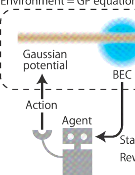
Figure 1: Schematic illustration of our system. The system consists of an agent and the environment. At each time step, the agent decides on an action on the environment, namely, how to change the external Gaussian potential applied to the BEC. The dynamics of the BEC with the time-dependent Gaussian potential is obtained by numerically solving the Gross-Pitaevskii (GP) equation, and the state of the BEC and the reward are given to the agent. The agent is trained to get a higher reward, which leads to the production of a desired state of the BEC.

Figure 1 illustrates reinforcement learning to control a BEC. We aim to create and manipulate quantized vortices in a BEC by changing a Gaussian external potential. Experimentally, such a potential can be produced by a nonresonant Gaussian laser beam applied to the BEC. On the environmental side, the dynamics of the BEC with a time-dependent Gaussian external potential are obtained by numerically solving the Gross-Pitaevskii (GP) equation. At each time step, the agent obtains the state of the BEC from the environment, and decides on the next action, i.e., how to change the position, strength, and shape of the Gaussian potential. The decision of the agent is made using a deep convolutional neural network (CNN), where the spatial distributions of the density and velocity of the BEC are directly input into the CNN, giving the next action as an output. At each time step, the agent also receives reward from the environment. The reward is higher when the state of the BEC is closer to the target state. The CNN of the agent is trained to maximize the total amount of rewards, which enables the agent to discover an optimal control of the Gaussian potential.

Using the above scheme, we demonstrate that quantized vortices can be created and manipulated in two-dimensional (2D) and three-dimensional (3D) BECs. In a 2D system, the target state is set to be the state with a singly-quantized vortex at the center. Although both vortices and antivortices are created in pairs by a simple translation of the Gaussian potential [41, 42], the agent finds a clever way to generate a single vortex state. In a 3D system, the target state is set to be the stationary vortex-ring state, and the agent finds that it can be created by a simple Gaussian laser beam.

The remainder of the paper is organized as follows. Section 2 explains our method, Sec. 3 shows the numerical results, and Sec. 4 gives the conclusions to this study.

2 Method

2.1 Environment

We begin by describing the environment of the reinforcement learning system. As described above, the environment receives the action from the agent and evolves to the next time step depending on the action. The environment then relays its state to the agent. The environment also evaluates whether the action of the agent was a good action, and gives a reward to the agent.

As an environment, we consider a BEC of bosonic atoms with mass $m$ confined in a harmonic potential. In the mean-field approximation at zero temperature, the macroscopic wave function $\psi(\bm{r},t)$ obeys the GP equation given by

$$i\hbar\frac{\partial\psi}{\partial t}=-\frac{\hbar^{2}}{2m}\nabla^{2}\psi+V_{\rm trap}(\bm{r})\psi+V_{G}(\bm{r},t)\psi+g|\psi|^{2}\psi,$$ (1)

where $V_{\rm trap}=m[\omega_{\perp}^{2}(x^{2}+y^{2})+\omega_{z}^{2}z^{2}]/2$ is the harmonic trap potential with $\omega_{\perp}$ and $\omega_{z}$ being the radial and axial trap frequencies, $V_{G}$ is the Gaussian external potential, and $g=4\pi\hbar^{2}a/m$ is the interaction coefficient with $a$ being the $s$-wave scattering length of the atom. The wave function is normalized as $\int|\psi|^{2}d\bm{r}=N_{\rm atom}$, where $N_{\rm atom}$ is the number of atoms.

In the next section, we will investigate both 2D and 3D systems. For the 3D system, for simplicity, the harmonic trap potential is assumed to be isotropic, i.e., $\omega_{\perp}=\omega_{z}\equiv\omega$. The external Gaussian potential for the 3D problem has the form

$$V_{G}(\bm{r},t)=A(t)\exp\left\{\frac{y^{2}}{d_{y}^{2}(t)}+\frac{[z-\zeta(t)]^{2}}{d_{z}^{2}}\right\},$$ (2)

where the strength $A(t)>0$, width $d_{y}(t)>0$, and position $\zeta(t)$ are control parameters, and the width $d_{z}$ is a constant. Such an external potential can be produced by a blue-detuned Gaussian laser beam propagating in the $x$ direction.

The 2D system is experimentally realized by tight confinement in the $z$ direction such that $\hbar\omega_{z}$ is much larger than the other characteristic energies. In this case, the wave function can be approximated as $\psi(\bm{r},t)=\psi_{\perp}(x,y,t)\psi_{0}(z)e^{-i\omega_{z}t/2}$, where $\psi_{0}(z)$ is the ground state of the harmonic oscillator potential $m\omega_{z}^{2}z^{2}/2$. Multiplying Eq. (1) by $\psi_{0}(z)$ and integrating it with respect to $z$, the system is reduced to 2D as

$$i\hbar\frac{\partial\psi_{\perp}}{\partial t}=-\frac{\hbar^{2}}{2m}\nabla_{\perp}^{2}\psi_{\perp}+V_{\rm trap}(x,y)\psi_{\perp}+V_{G}(x,y,t)\psi_{\perp}+g_{\perp}|\psi_{\perp}|^{2}\psi_{\perp},$$ (3)

where $\nabla_{\perp}^{2}=\partial^{2}/\partial x^{2}+\partial^{2}/\partial y^{2}$, $V_{\rm trap}(x,y)=m\omega_{\perp}^{2}(x^{2}+y^{2})/2$, and $g_{\perp}=[m\omega_{z}/(2\pi\hbar)]^{1/2}g$. The external Gaussian potential for the 2D problem is assumed to be

$$V_{G}(x,y,t)=A_{\perp}(t)\exp\left\{\frac{[x-\xi(t)]^{2}}{d^{2}}+\frac{[y-\eta(t)]^{2}}{d^{2}}\right\},$$ (4)

where the strength $A_{\perp}(t)>0$ and position $\xi(t)$, $\eta(t)$ are control parameters, and the width $d$ is a constant. This form of the potential is generated by a blue-detuned Gaussian laser beam propagating in the $z$ direction.

At the start of each run of time evolution (called an episode), the environment is reset: the control parameters are set to the initial values, and the wave function is set to the ground state for $V_{G}(t=0)$. The ground-state wave function is prepared by the imaginary-time evolution, where $i$ on the right-hand sides of Eqs. (1) and (3) is replaced with $-1$. The real-time and imaginary-time evolution is numerically obtained by the pseudospectral method [43]. After the initial reset of the environment, the real-time evolution starts. At intervals of time $\Delta t$ (which is much larger than the discretized time interval $\delta t$ in the pseudospectral method), the environment returns its state and the reward to the agent, and receives the action from the agent (see Fig. 1). The state of the environment given to the agent is the density distribution $\rho=|\psi|^{2}$ and flux distribution $\bm{F}=\hbar(\psi^{*}\bm{\nabla}\psi-\psi\bm{\nabla}\psi^{*})/(2mi)$ ($\psi\rightarrow\psi_{\perp}$ for 2D) of the BEC. The state of the environment also includes the current shape of the Gaussian potential $V_{G}$ so that the agent can determine how to change the potential. The reward given to the agent is calculated from the overlap between the current wave function and the target wave function, which is specified in the next section. By the action received from the agent, one of the parameters in the Gaussian external potential is changed by a small amount at each time step. Each episode terminates at $t=500\Delta t\equiv T_{\rm end}$, which is followed by the next episode.

2.2 Agent

The agent observes the state $s_{t}$ of the environment at time $t$, and determines the action $a_{t}$ on the environment. The agent then gets the reward $r_{t}$ for the action from the environment. From these experiences, the agent tries to maximize the discounted cumulative reward, $\sum_{n=0}^{\infty}\gamma^{n}r_{t+n\Delta t}$, where $0<\gamma<1$ is the discount rate [44].

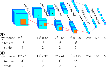
Figure 2: Structures of the CNNs for the 2D and 3D cases. The density and flux distributions of the BEC and the Gaussian potential distribution are input into the CNN. The six values from the output correspond to $Q(s_{t},a)$ for six actions $a=0,1,\cdots,5$. Filters are applied with the indicated stride and without padding in each convolutional layer. There are no pooling layers.

As mentioned in Sec. 2.1, as the state $s_{t}$ of the environment, we take the density distribution $\rho(\bm{r},t)$, flux distribution $\bm{F}(\bm{r},t)$, and the Gaussian potential $V_{G}(\bm{r},t)$. For the 2D case, the four distributions $\rho(x,y)$, $F_{x}(x,y)$, $F_{y}(x,y)$, and $V_{G}(x,y)$ are expressed by $64\times 64\times 4$ pixels, and are input into the CNN [45] shown in Fig. 2. For the 3D case, the five distributions $\rho(x,y,z)$, $F_{x}(x,y,z)$, $F_{y}(x,y,z)$, $F_{z}(x,y,z)$, and $V_{G}(x,y,z)$ are expressed by $32\times 32\times 32\times 5$ pixels. The CNN consists of four convolutional layers and two fully-connected layers. The CNN outputs six values, which we denote $Q(s_{t},a)$ with $a=0,1,\cdots,5$. The agent determines the action $a_{t}$ by the $\epsilon$-greedy policy:

$$a_{t}=\left\{\begin{array}[]{cc}\mbox{randomly chosen from 0 to 5}&(r<\epsilon)\\ \mbox{argmax}_{a}Q(s_{t},a)&(r\geq\epsilon),\end{array}\right.$$ (5)

where $0\leq r<1$ is a random number and $\mbox{argmax}_{a}Q(s_{t},a)$ indicates the value of $a$ that maximizes $Q(s_{t},a)$. The value of $\epsilon$ is linearly decreased from 1 to 0.1 in the first 50,000 steps (100 episodes), and a constant value of $\epsilon=0.1$ is used after that. The action $a_{t}$ chosen by the agent is applied to the environment, where the Gaussian external potential is changed depending on $a_{t}$, and the BEC evolves from $t$ to $t+\Delta t$. The agent then receives the reward $r_{t}$ from the environment, and observes the new state $s_{t+\Delta t}$.

According to the Bellman optimality equation [44], $Q(s_{t},a_{t})$ should approach the target value $r_{t}+\gamma Q(s_{t+\Delta t},a^{\prime})$, where $a^{\prime}=\mbox{argmax}_{a}Q(s_{t+\Delta t},a)$. It was reported in Ref. Hasselt that the training process is stabilized by replacing $Q$ with $\hat{Q}$ in the above target value, where $\hat{Q}$ is generated by another CNN, called the target network. Thus, the target value is given by

$$y_{t}=r_{t}+\gamma\hat{Q}(s_{t+\Delta t},\mbox{argmax}_{a}Q(s_{t+\Delta t},a)).$$ (6)

The original CNN to generate $Q$ is updated in every training step, and the original CNN is copied to the target CNN every $C$ steps, where we take $C=1000$. The target value $y_{t}$ is thus calculated by fixing the target CNN during $C$ steps, which stabilizes the learning process. This method with Eq. (6) is called double-Q learning [46].

The agent (CNN) is trained as follows. In every time step, the set of data $(s_{t},a_{t},r_{t},s_{t+\Delta t})$ is stored in the memory, which is called the replay memory [3]. In the present case, the replay memory can store 50,000 sets of data. Once the limit is reached, old data are removed to store new data (queue). From the replay memory, 32 sets of data are taken randomly, which is called a minibatch. For each dataset in the minibatch, the target value $y_{t}$ in Eq. (6) is calculated, and the network parameters of the CNN are updated to minimize $\sum_{\rm minibatch}L(Q(s_{t},a_{t})-y_{t})$, where the function $L$ is called the Huber loss [47], defined by

$$L(x)=\left\{\begin{array}[]{cc}\frac{x^{2}}{2}&(|x|\leq 1)\\ |x|-\frac{1}{2}&(|x|>1).\end{array}\right.$$ (7)

Using the Huber loss, large gradients are suppressed and network updates are stabilized. Updating the CNN is performed using the Adam optimization scheme [48] with a learning rate of $10^{-5}$-$10^{-4}$. The procedure for the agent is summarized in Algorithm 1.

Algorithm 1

  Initialize deep-Q network $Q$

  Initialize target network as $\hat{Q}=Q$

  for episode = 1, $N_{\rm episode}$ do

     Initialize environment and get initial observation $s_{0}$

     for $t=0$, $T_{\rm end}$ do

        Select action $a_{t}={\rm argmax}_{a}Q(s_{t},a)$ with $\epsilon$-greedy exploration

        Execute action $a_{t}$ on environment and get reward $r_{t}$ and next state $s_{t+\Delta t}$

        Store $(s_{t},a_{t},r_{t},s_{t+\Delta t})$ in replay memory

        Sample minibatch of $(s_{t},a_{t},r_{t},s_{t+\Delta t})$ from replay memory

        Set $y_{t}=r_{t}$ if $t=T_{\rm end}$, otherwise $y_{t}=r_{t}+\gamma\hat{Q}(s_{t+\Delta t},a^{\prime})$, where $a^{\prime}={\rm argmax}_{a}Q(s_{t+\Delta t},a)$

        Train network using gradient of $L(y_{t}-Q(s_{t},a_{t}))$

        Copy $\hat{Q}=Q$ every $C$ steps

     end for

  end for

3 Results

We numerically demonstrate that our method can create and manipulate vortices in BECs. In the following, we normalize the length, time, and energy by $[\hbar/(m\omega_{\perp})]^{1/2}$, $\omega_{\perp}^{-1}$, and $\hbar\omega_{\perp}$, respectively. The density $|\psi_{\perp}|^{2}$ is normalized by $N_{\rm atom}m\omega_{\perp}/\hbar$ in 2D, and $|\psi|^{2}$ is normalized by $N_{\rm atom}(m\omega_{\perp}/\hbar)^{3/2}$ in 3D. For 2D calculations, the normalized interaction coefficient $\tilde{g}_{\perp}=N_{\rm atom}a(8\pi m\omega_{z}/\hbar)^{1/2}$ is taken to be 1000. For example, for ${}^{87}{\rm Rb}$ atoms in a quasi-2D trap with $\omega_{\perp}=2\pi\times 100$ Hz and $\omega_{z}=2\pi\times 10$ kHz, $\tilde{g}_{\perp}=1000$ corresponds to $N_{\rm atom}\simeq 4.1\times 10^{3}$. For 3D calculations, the normalized interaction coefficient $\tilde{g}=4\pi N_{\rm atom}a(m\omega_{\perp}/\hbar)^{1/2}$ is taken to be 6000. For a 3D isotropic trap with $\omega=2\pi\times 100$ Hz, $\tilde{g}=6000$ corresponds to $N_{\rm atom}=9.7\times 10^{4}$. The spatial discretization size is 0.15 with a $128\times 128$ mesh for the 2D case, and 0.25 with a $64\times 64\times 64$ mesh for the 3D case. These spatial data are averaged and reduced to $64\times 64$ for the 2D case and $32\times 32\times 32$ for the 3D case to be input into the CNN in Fig. 2. The time interval for numerical integration is $\delta t=0.002$, and the time step for the reinforcement learning is $\Delta t=50\delta t=0.1$.

3.1 Two-dimensional system

We first consider the 2D system, which obeys the GP equation in Eq. (3). The initial parameters of the Gaussian potential in each episode are $\xi(0)=0$, $\eta(0)=2$, and $A_{\perp}(0)=20$. The initial state of the BEC is the ground state for these parameters, as shown in Fig. 3(a), where the density dip is due to the Gaussian potential. For this initial state, therefore, the rotational symmetry of the problem is broken. Here we set our target state $\psi_{\rm target}(x,y)$ to the lowest-energy stationary state having a singly-quantized counterclockwise vortex at the center, as shown in Fig. 3(f). Numerically, such a wave function can be obtained by phase imprinting followed by imaginary-time evolution. Starting from the initial state without a vortex, the agent tries to produce $\psi_{\rm target}(x,y)$ by controlling the position and strength of the Gaussian potential in Eq. (4).

We specify the action and reward. Depending on the six actions of the agent, $a=0,1,\cdots,5$, the parameters in Eq. (4) are changed in each time step as

$$\begin{array}[]{cc}a=0&\xi\rightarrow\xi+0.15,\\ a=1&\xi\rightarrow\xi-0.15,\\ a=2&\eta\rightarrow\eta+0.15,\\ a=3&\eta\rightarrow\eta-0.15,\\ a=4&A_{\perp}\rightarrow A_{\perp}+2,\\ a=5&A_{\perp}\rightarrow A_{\perp}-2,\end{array}$$ (8)

where the displacement 0.15 is identical with the numerical mesh size. Since the strength $A_{\perp}$ of the Gaussian potential produced by a blue-detuned laser beam should be nonnegative, the actions $a=5$ is ignored when $A_{\perp}$ becomes negative. The fidelity between the wave function $\psi_{\perp}(x,y,t)$ at time $t$ and the target wave function $\psi_{\rm target}(x,y)$ is defined by

$$F(t)=\left|\int\psi_{\rm target}^{*}(x,y)\psi_{\perp}(x,y,t)dxdy\right|^{2}.$$ (9)

Since the present purpose is to increase the fidelity as much as possible, the reward $r_{t}$ given to the agent should be taken to be a monotonically increasing function of the fidelity. Here, to enhance the increase of the fidelity near $F=1$, we take the reward as

$$r_{t}=F(t)+8[F(t)]^{16}.$$ (10)

As shown in the inset of Fig. 3(g), this function steeply rises for $F\gtrsim 0.9$.

Figure 3: Result with the best total reward through 5000 trials of episodes. (a)-(e) Snap shots of the density profiles in the time evolution. The crosses and circles in (c) and (d) indicate the positions of clockwise and counterclockwise vortex cores, respectively. (f) Density profile of the target state, which has a counterclockwise vortex at the center. (g) Parameters $\xi(t)$, $\eta(t)$, and $A_{\perp}(t)$ of the Gaussian external potential. The inset in (g) plots Eq. (10). See the Supplemental Material for a movie of the dynamics shown in (a)-(e) [49].

We performed the reinforcement learning in Algorithm 1 for $N_{\rm episode}=5000$ episodes. The total reward obtained in each episode is defined as

$$R_{\rm total}=\sum_{n=0}^{500}r_{n\Delta t},$$ (11)

where the episode terminates at $T_{\rm end}=500\Delta t$. The episode with the largest $R_{\rm total}$ among 5000 episodes is shown in Fig. 3. First, the Gaussian potential is moved leftward (Fig. 3(b)), and at the edge of the BEC a clockwise vortex is released to the periphery of the BEC, leaving a counterclockwise vortex in the Gaussian potential (Fig. 3(c)). The Gaussian potential then carries the counterclockwise vortex to the center of the BEC (Fig. 3(d)), at which point the strength of the Gaussian potential is reduced to produce the desired state (Fig. 3(e)). This process finishes at $t\simeq 130$, and after that the vortex is kept at the center. It is numerically predicted [41] and experimentally verified [42] that the simple translation of a circular potential in a BEC produces a pair of clockwise and counterclockwise vortices simultaneously. In the above dynamics, in contrast, the strong anisotropy at the edge of the condensate is used to release only a single vortex from the potential.

Figure 3(g) shows the time dependence of the controlled parameters $\xi(t)$, $\eta(t)$, and $A(t)$. The strength $A(t)$ of the Gaussian potential is first decreased from the initial value as the potential goes to the edge of the BEC. This is because the density is low at the edge of the BEC and a weak Gaussian potential is suitable for manipulating the vortices. The strength $A(t)$ is then increased to rapidly transport the counterclockwise vortex to the center. Even after the final state is produced at $t\simeq 130$, $A(t)$ is kept at $\simeq 4$, which helps fix the vortex to the center. It was confirmed that the vortex stays almost at the center, even if $A(t)$ vanishes for $t\geq 130$.

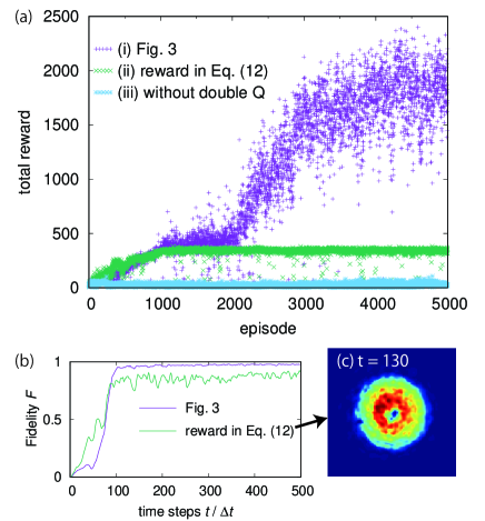
Figure 4: (a) Total reward in Eq. (11) obtained in each episode in the learning process. (i) The learning process with 5000 episodes. The episode with the largest total reward is used in Fig. 3. (ii) Using the reward in Eq. (12) instead of Eq. (10). (iii) Using the target value in Eq. (13) instead of the double-Q learning in Eq. (6). (b) Time evolution of the fidelity for the episode with the best total reward for conditions (i) and (ii). (c) Snapshot of the density profile for case (ii) in (b).

Figure 4(a) shows the total reward $R_{\rm total}$ obtained in each episode. The total reward increases as the agent experiences more episodes, and finally reaches $R_{\rm total}\simeq 2000$. The total reward first increases to $R_{\rm total}\simeq 400$, then remains on a plateau till the $\simeq 2000$th episodes and then increases again. This behavior is related to the form of the reward in the inset in Fig. 3(g), because the total reward saturates at $R_{\rm total}\simeq 400$ if we replace the reward in Eq. (10) with

$$r_{t}=F(t).$$ (12)

Figure 4(b) shows the time evolution of the fidelity $F(t)$ for the best episode, which indicates that the fidelity reaches $F\simeq 0.97$ using the reward in Eq. (10), while $F\simeq 0.9$ for the reward in Eq. (12). A snapshot of the density profile for the reward in Eq. (12) is shown in Fig. 4(c), which exhibits more short-wavelength excitations than Fig. 3(e). Thus, the nonlinear term in Eq. (10) makes the fidelity closer to unity, and reduces short-wavelength excitations. In Fig. 4(a), we also show the case without double-Q learning, i.e., we use

$$y_{t}=r_{t}+\gamma Q(s_{t+\Delta t},\mbox{argmax}_{a}Q(s_{t+\Delta t},a))$$ (13)

instead of Eq. (6). Without the target network $\hat{Q}$, the learning process does not proceed, which indicates the validity of the target network.

3.2 Three-dimensional system

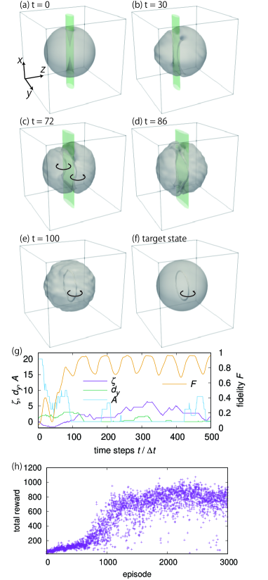
Figure 5: (a)-(e) Dynamics of a 3D BEC with the best total reward. The BEC is confined in an isotropic harmonic trap with an external Gaussian potential in Eq. (2). (f) Target state containing a stationary vortex ring. The arrows indicate the directions of circulation. Surfaces of equal density $|\psi|^{2}=0.0005$ are shown in gray and surfaces of equal Gaussian potential $V_{G}=3$ are shown in green (dark gray). The size of the cubic frames is $16\times 16\times 16$. (g) Parameters $\zeta(t)$, $d_{y}(t)$, and $A(t)$ of the Gaussian external potential used in (a)-(e). For $t/\Delta t\gtrsim 100$, the Gaussian potential almost vanishes, since $A(t)\simeq 0$ or $d_{y}(t)\simeq 0$. The time evolution of the fidelity $F(t)$ defined in Eq. (15) is also shown. (h) Total reward obtained in each episode in the learning process. The episode with the best total reward among these 3000 episodes is used in (a)-(e) and (g). See the Supplemental Material for a movie of the dynamics shown in (a)-(e) [51].

Next, we consider a 3D system obeying Eq. (1), in which a BEC is confined in an isotropic harmonic potential, and a Gaussian laser beam is applied from the $x$ direction, producing the potential in Eq. (2). The initial parameters in Eq. (2) are set to $A(0)=20$, $d_{y}(0)=1$, and $\zeta(0)=0$, and $d_{z}=0.5$ is fixed. The initial wave function is the ground state for these parameters, as shown in Fig. 5(a). Here, our target state $\psi_{\rm target}(\bm{r})$ is the stationary state containing a vortex ring [50] with axial symmetry about the $z$ axis, as shown in Fig. 5(f). Although a vortex ring in a uniform system travels in the direction of the symmetry axis, the vortex ring in Fig. 5(f) is stationary due to the inhomogeneity. Numerically, this target state is generated by imprinting the phase $e^{i\phi}$ with $\phi=\tan^{-1}[z/(r_{\perp}-r_{0})]-\tan^{-1}[z/(r_{\perp}+r_{0})]$ followed by the imaginary-time evolution, where $r_{0}$ and the duration of the imaginary-time evolution are chosen appropriately.

As in the 2D case, the agent chooses one of six actions, $a=0,1,\cdots,5$, according to which the parameters of the Gaussian potential are modified as

$$\begin{array}[]{cc}a=0&\zeta\rightarrow\zeta+0.15,\\ a=1&\zeta\rightarrow\zeta-0.15,\\ a=2&d_{y}\rightarrow d_{y}+0.2,\\ a=3&d_{y}\rightarrow d_{y}-0.2,\\ a=4&A\rightarrow A+2,\\ a=5&A\rightarrow A-2,\end{array}$$ (14)

in each time step. The actions $a=3$ and 5 are ignored when $d_{y}$ and $A$ become negative, respectively. The reward has the same form as in Eq. (10) with the fidelity being given by

$$F(t)=\left|\int\psi^{*}_{\rm target}(\bm{r})\psi(\bm{r},t)d\bm{r}\right|^{2}.$$ (15)

Figures 5(a)-5(e) show the time evolution of the BEC for the episode with the best total reward among $N_{\rm episode}=3000$ episodes. The controlled parameters of the Gaussian external potential are shown in Fig. 5(g). First, the Gaussian potential is moved in the $-z$ direction, and a pair of vortex-antivortex lines are produced (Fig. 5(b)). The width $d_{y}$ of the Gaussian potential is then increased (Fig. 5(c)), and the two vortex lines connect with each other at the $\pm x$ edges (Fig. 5(d)), which forms a vortex ring (Fig. 5(e)). The produced vortex ring is almost stationary and stays in the condensate until the end of the episode $t/\Delta t=500$. After $t/\Delta t\gtrsim 100$, the Gaussian external potential almost vanishes because either $A=0$ or $d_{y}=0$.

The generation of the vortex ring shown above is nontrivial, because the external Gaussian potential is uniform in the $x$ direction. In a uniform system, using such a potential, we can only generate vortex lines along the $x$ direction, and therefore the vortex-ring formation in our system is due to the inhomogeneity in the trap. The board-like potential with large $d_{y}$, as in Figs. 5(c) and 5(d), also plays an important role. This potential creates the constrictions at the $\pm x$ edges of the isodensity surface, as shown in Fig. 5(c), which bend the vortex lines and forms a ring.

The time evolution of the fidelity $F(t)$ is shown in Fig. 5(g). Unlike the 2D case in Fig. 4(b), the fidelity in Fig. 5(g) exhibits nonadiabatic oscillation, which may be unavoidable for the present condition. Figure 5(h) shows the total reward $R_{\rm total}$ obtained in each episode. The total reward first increases gradually for $\lesssim 1000$th step and then suddenly rises to $R_{\rm total}\simeq 800$. This behavior is similar to that in the 2D case shown in Fig. 4(a).

4 Conclusions and discussions

We have applied reinforcement learning to the control of nonlinear matter waves. The agent in the reinforcement learning is implemented using a deep convolutional neural network (CNN), and the state of the Bose-Einstein condensate (BEC) is input into the CNN to determine the next action of the agent. According to the action of the agent, the position and shape of the external Gaussian potential applied to the BEC are controlled. The agent is trained so that the state of the BEC approaches the prescribed target state.

Using this method, we demonstrated that quantized vortices can be created and manipulated in 2D and 3D systems. In the 2D system, the target state was set to be the single-vortex state at the center. Although vortices and antivortices are always created in pairs, the agent found a way to expel one of them to leave only a single vortex at the center of the BEC (Fig. 3). In the 3D system, the target state was set to be the stationary vortex-ring state. Although the Gaussian potential is 2D (uniform in the $x$ direction), the agent found a way to produce such a 3D structure (Fig. 5).

The two examples demonstrated in the present paper are interesting, but rather simple; the control parameters found in Figs. 3(g) and 5(g) for creating the target states are very simple functions. Other methods have been developed to control quantum systems [33, 34, 35] that may find similar optimal results. Furthermore, the simple vortex states used for our target states can also be created by other methods, such as methods using Rabi transitions [52, 53]. In this sense, our method might be considered overcomplicated for the present examples. However, reinforcement learning is very versatile and may prove to be an effective approach for handling more complicated problems (e.g., manipulation of multiple vortex states, control of quantum turbulence, creation of nontrivial topological excitations, etc.). This will be the topic of future studies.

Another challenging extension of this study will be the real-time control of BECs in experiments, where a series of nondestructive imaging data is given to the agent, and the reward is based on the measurement data. Reinforcement learning may be suitable for such measurement-based control which introduces errors and noise, since the method has already been successfully applied to control real-world objects, such as robots.

- [1] D. Silver, A. Huang, C. J. Maddison, A. Guez, L. Sifre, G. van den Driessche, J. Schrittwieser, I. Antonoglou, V. Panneershelvam, M. Lanctot, S. Dieleman, D. Grewe, J. Nham, N. Kalchbrenner, I. Sutskever, T. Lillicrap, M. Leach, K. Kavukcuoglu, T. Graepel, and D. Hassabis, Nature 529, 484 (2016).
- [2] D. Silver, J. Schrittwieser, K. Simonyan, I. Antonoglou, A. Huang, A. Guez, T. Hubert, L. Baker, M. Lai, A. Bolton, Y. Chen, T. Lillicrap, F. Hui, L. Sifre, G. van den Driessche, T. Graepel, and D. Hassabis, Nature 550, 354 (2017).
- [3] V. Mnih, K. Kavukcuoglu, D. Silver, A. A. Rusu, J. Veness, M. G. Bellemare, A. Graves, M. Riedmiller, A. K. Fidjeland, G. Ostrovski, S. Petersen, C. Beattie, A. Sadik, I. Antonoglou, H. King, D. Kumaran, D. Wierstra, S. Legg, and D. Hassabis, Nature 518, 529 (2015).
- [4] C. Chen, D. Dong, H.-X. Li, J. Chu, and T.-J. Tarn, IEEE Trans. Neural Netw. Learn. Syst. 25, 920 (2014).
- [5] M. Bukov, A. G. R. Day, D. Sels, P. Weinberg, A. Polkovnikov, and P. Mehta, Phys. Rev. X 8, 031086 (2018).
- [6] M. Bukov, Phys. Rev. B 98, 224305 (2018).
- [7] F. Albarrán-Arriagada, J. C. Retamal, E. Solano, and L. Lamata, Phys. Rev. A 98, 042315 (2018).
- [8] S. Yu, F. Albarrán-Arriagada, J. C. Retamal, Y.-T. Wang, W. Liu, Z.-J. Ke, Y. Meng, Z.-P. Li, J.-S. Tang, E. Solano, L. Lamata, C.-F. Li, and G.-C. Guo, Adv. Quantum Technol. 2, 1800074 (2019).
- [9] T. Fösel, P. Tighineanu, T. Weiss, and F. Marquardt, Phys. Rev. X 8, 031084 (2018).
- [10] X.-M. Zhang, Z.-W. Cui, X. Wang, and M.-H. Yung, Phys. Rev. A 97, 052333 (2018).
- [11] P. Andreasson, J. Johansson, S. Liljestrand, and M. Granath, Quantum 3, 183 (2019).
- [12] F. Chen, J.-J. Chen, L.-N. Wu, Y.-C. Liu, and L. You, Phys. Rev. A 100, 041801(R) (2019).
- [13] M. August, J. M. Hernández-Lobato, arXiv:1802.04063.
- [14] M. Y. Niu, S. Boixo, V. Smelyanskiy, and H. Neven, arXiv:1803.01857.
- [15] J.-J. Chen and M. Xue, arXiv:1901.08748.
- [16] Z. T. Wang, Y. Ashida, and M. Ueda, arXiv:1910.09200
- [17] J. Mackeprang, D. Dasari, and J. Wrachtrup, arXiv:1908.05981.
- [18] U. Hohenester, P. K. Rekdal, A. Borzí, and J. Schmiedmayer, Phys. Rev. A 75, 023602 (2007).
- [19] X. Chen, E. Torrontegui, D. Stefanatos, J.-S. Li, and J. G. Muga, Phys. Rev. A 84, 043415 (2011).
- [20] S. Amri, R. Corgier, D. Sugny, E. M. Rasel, N. Gaaloul, and E. Charron, Sci. Rep. 9, 5346 (2019).
- [21] G. Jäger, D. M. Reich, M. H. Goerz, C. P. Koch, and U. Hohenester, Phys. Rev. A 90, 033628 (2014).
- [22] J.-F. Mennemann, D. Matthes, R.-M. Weishäupl, and T. Langen, New J. Phys. 17, 113027 (2015).
- [23] J. Grond, J. Schmiedmayer, and U. Hohenester, Phys. Rev. A 79, 021603(R) (2009).
- [24] G. Jäger, T. Berrada, J. Schmiedmayer, T. Schumm, and U. Hohenester, Phys. Rev. A 92, 053632 (2015).
- [25] R. Bücker, T. Berrada, S. van Frank, J.-F. Schaff, T. Schumm, J. Schmiedmayer, G. Jäger, J. Grond, and U. Hohenester, J. Phys. B 46, 104012 (2013).
- [26] S. van Frank, M. Bonneau, J. Schmiedmayer, S. Hild, C.Gross, M. Cheneau, I. Bloch, T. Pichler, A. Negretti, T. Calarco, and S. Montangero, Sci. Rep. 6, 34187 (2016).
- [27] D. Hocker, J. Yan, and H. Rabitz, Phys. Rev. A 93, 053612 (2016).
- [28] C. A. Weidner and D. Z. Anderson, Phys. Rev. Lett. 120, 263201 (2018).
- [29] J. J. W. H. Sørensen, M. O. Aranburu, T. Heinzel, and J. F. Sherson, Phys. Rev. A 98, 022119 (2018).
- [30] M. K. Riahi, J. Salomon, S. J. Glaser, and D. Sugny, Phys. Rev. A 93, 043410 (2016).
- [31] J. C. Saywell, I. Kuprov, D. Goodwin, M. Carey, and T. Freegarde, Phys. Rev. A 98, 023625 (2018).
- [32] J.-F. Mennemann, T. Langen, L. Exl, and N. J. Mauser, Comput. Phys. Commun. 244, 205 (2019).
- [33] N. Khaneja, T. Reiss, C. Kehlet, T. Schulte-Herbrüggen, and S. J. Glaser, J. Magn. Reson. 172, 296 (2005).
- [34] P. Doria, T. Calarco, and S. Montangero, Phys. Rev. Lett. 106, 190501 (2011).
- [35] T. Caneva, T. Calarco, and S. Montangero, Phys. Rev. A 84, 022326 (2011).
- [36] P. B. Wigley, P. J. Everitt, A. van den Hengel, J. W. Bastian, M. A. Sooriyabandara, G. D. McDonald, K. S. Hardman, C. D. Quinlivan, P. Manju, C. C. N. Kuhn, I. R. Petersen, A. N. Luiten, J. J. Hope, N. P. Robins, and M. R. Hush, Sci. Rep. 6, 25890 (2016).
- [37] I. Nakamura, A. Kanemura, T. Nakaso, R. Yamamoto, and T. Fukuhara, Opt. Exp. 27, 20435 (2019).
- [38] A. J. Barker, H. Style, K. Luksch, S. Sunami, D. Garrick, F. Hill, C. J. Foot, and E. Bentine, Mach. Learn.: Sci. Technol. 1, 015007 (2020).
- [39] E. T. Davletov, V. V. Tsyganok, V. A. Khlebnikov, D. A. Pershin, D. V. Shaykin, and A. V. Akimov, arXiv:2003.00346
- [40] B. M. Henson, D. K. Shin, K. F. Thomas, J. A. Ross, M. R. Hush, S. S. Hodgman, and A. G. Truscott, PNAS 115, 13216 (2018).
- [41] T. Frisch, Y. Pomeau, and S. Rica, Phys. Rev. Lett. 69, 1644 (1992).
- [42] T. W. Neely, E. C. Samson, A. S. Bradley, M. J. Davis, and B. P. Anderson, Phys. Rev. Lett. 104, 160401 (2010).
- [43] W. H. Press, S. A. Teukolsky, W. T. Vetterling, and B. P. Flannery, Numerical Recieps, 3rd ed. (Cambridge Univ. Press, Cambridge, 2007).
- [44] R. S. Sutton and A. G. Barto, Reinforcement Learning, 2nd ed., (MIT Press, Cambridge, 2018)
- [45] I. Goodfellow, Y. Bengio, and A. Courville, Deep learning (MIT Press, Massachusetts, 2016)
- [46] H. van Hasselt, A. Guez, and D. Silver, arXiv:1509.06461.
- [47] P. J. Huber, Ann. Math. Statist. 35, 73 (1964).
- [48] D. P. Kingma and J. L. Ba, arXiv:1412.6980.
- [49] (Supplemental Material) A movie of the dynamics in Fig. 3(b)-3(f) is provided online.
- [50] L.-C. Crasovan, V. M. Pérez-García, I. Danaila, D. Mihalache, and L. Torner, Phys. Rev. A 70, 033605 (2004).
- [51] (Supplemental Material) A movie of the dynamics in Fig. 5(b)-5(f) is provided online.
- [52] M. F. Anderson, C. Ryu, P. Cladé, V. Natarajan, A. Vaziri, K. Helmerson, and W. H. Phillips, Phys. Rev. Lett. 97, 170406 (2006).
- [53] J. Ruostekoski and J. R. Anglin, Phys. Rev. Lett. 86, 3934 (2001).