Efficient Linear Transmission Strategy for MIMO Relaying Broadcast Channels with Direct Links

Abstract

In this letter, a novel linear transmission strategy to design the linear precoding matrix (PM) at base station (BS) and the beamforming matrix (BM) at relay station (RS) for multiple-input multiple-output (MIMO) relaying broadcast channels with direct channel (DC) is proposed, in which a linear PM is designed at BS based on DC, and the RS utilizes the PM, the backward channel and the forward channel to design the linear BM. We then give a quite tight lower bound of the achievable sum-rate of the network with the proposed strategy to measure the performance. The sum-rates achieved by the proposed strategy is compared with other schemes without considering the DC in design in simulations, which shows that the proposed strategy outperforms the existing methods when RS is close to BS.

I Introduction

Recently, MIMO relaying broadcast network has attracted considerable interest from both academic and industrial communities. For a MIMO relaying broadcast network, there are two independent channels between source and destination nodes; i.e., relay channel consisting of backward channel (BC) and forward channel (FC), and direct channel (DC). Many works [1, 2, 3, 4, 5, 6, 7] have investigated the linear transmission strategy for MIMO relaying broadcast networks. In [1], an implementable multiuser precoding strategy that combines Tomlinson-Harashima precoding at the BS and linear signal processing at the RS is presented. In [2], a joint optimization of linear beamforming and power control at BS and RS to minimize the weighted sum-power consumption under the user minimum SINR-(QoS)-constraints is presented. In [3], the singular value decomposition (SVD) and zero forcing (ZF) precoder are respectively used to the BC and FC to optimize the joint precoding. The authors use an iterative method to show that the optimal precoding matrices always diagonalize the compound channel of the system. In [4], the authors use the quadratic programming to joint precoding optimization to maximize the system capacity. In [5], the authors propose a scheme based on duality of MIMO multiple access and broadcast channel to maximize the system capacity. In [6] and [7], the authors consider a robust linear beamforming scheme with a limited feedback.

However, all these works only consider the BC and FC to optimize precoding matrix (PM) and beamforming matrix (BM) to maximize the system performance. For a MIMO relay network with DC, jointly designing the PM and BM to maximize capacity or minimize the mean square error is much difficult, especially for a MIMO relaying broadcast networks. In this letter, we consider a MIMO relaying broadcast networks composing of one BS, one RS and multiple users with DC, and propose a novel linear transmission strategy to design the PM and BM. To avoid complexity, we consider the distributed design method. Firstly, the BS designes the linear PM based on DC only, Secondly, the RS utilizes the linear PM, BC and FC to design the BM. Simulation results demonstrates that the proposed strategy outperforms the existing methods when RS is close to BS.

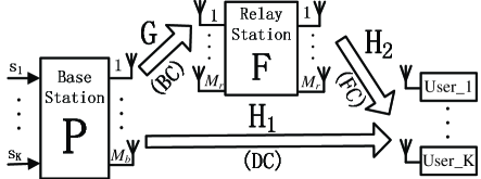
Figure 1: The MIMO relaying broadcast network with one base station, one relay station, and $K$ mobile users

Notations: $\textmd{E}(\cdot)$, $\mathrm{tr}(\cdot)$, $(\cdot)^{T}$, $(\cdot)^{-1}$, $(\cdot)^{{\dagger}}$, and $\mathrm{det}(\cdot)$ denote expectation, trace, inverse, transpose, conjugate transpose, and determinant, respectively. i.i.d stands for independent and identically distributed. $\mathbf{I}_{N}$ stands for an $N\times N$ identity matrix. $\mathrm{diag}(a_{1},\ldots,a_{N})$ is a diagonal matrix with the $i$th diagonal entry $a_{i}$. $\log$ is of base $2$. $\mathcal{C}^{M\times N}$ represents the set of $M\times N$ matrices over complex field, and $\sim\mathcal{CN}(x,y)$ means satisfying a circularly symmetric complex Gaussian distribution with mean $x$ and covariance $y$.

II System Model

In this letter, we consider the MIMO relaying broadcast channel with one BS, one RS, and $K$ single-antenna users as depicted in Fig 1. It is assumed that the BS and RS are equipped with $M_{b}$ and $M_{r}$ antennas, respectively. We consider that each user can receive the signals from the BS via DC and BC-FC. Assuming that the BS can support $K$ independent substreams for $K$ users simultaneously, which requires $K\leq M_{b}$. Here, we only consider $M_{b}=M_{r}=K$ for simplicity. By means of relaying scheme, we consider a non-regenerative and half-duplex relaying scheme applied at the RS to process and forward the received signals due to simplicity [8]. Thus, a broadcast transmission is composed of two phases. During the first phase, the BS broadcasts $K$ precoded data streams to the RS and users after applying a linear PM $\mathbf{P}$ to the data vector $\mathbf{s}$, where $\mathbf{s}=[s_{1},s_{2},\ldots,s_{K}]\sim\mathcal{CN}(0,\mathbf{I}_{K})$, $s_{k}$ is the symbol intended for the $k$th user. We supposed that the BS transmit power is $P_{s}$ and then the power control factor at the BS is $\rho_{s}=\sqrt{{P_{s}}/{\mathrm{tr}(\mathbf{P}\mathbf{P}^{{\dagger}})}}$ due to $\textmd{E}\{\mathbf{Ps}\mathbf{s}^{{\dagger}}\mathbf{P}^{{\dagger}}\}=\mathrm{tr}(\mathbf{P}\mathbf{P}^{{\dagger}})$. In this case, the received signal vectors at the users and RS are respectively

$$\mathbf{y}_{1} = [y_{11},y_{12},\ldots,y_{1K}]^{T}=\rho_{s}\mathbf{H}_{1}\mathbf{P}\mathbf{s}+\mathbf{n}_{1},$$ (1a)

$$\mathbf{y}_{r} = \rho_{s}\mathbf{G}\mathbf{P}\mathbf{s}+\mathbf{n}_{r},$$ (2a)

where $\mathbf{P}=[\mathbf{p}_{1},\mathbf{p}_{2},\ldots,\mathbf{p}_{k}]\in\mathcal{C}^{M_{b}\times K}$ is a PM at BS, and $\mathbf{H}^{T}_{1}=[\mathbf{h}_{11},\mathbf{h}_{12},\ldots,\mathbf{h}_{1k}]\in\mathcal{C}^{K\times M_{b}}$ is the DC matrix, in which $\mathbf{h}_{1k}$ is the channel vector between BS and the $k$th user. $\mathbf{G}$ is the BC matrix. Each entry in $\mathbf{H}_{1}$ and $\mathbf{G}$ is i.i.d complex Gaussian variables with zero mean and variances $\sigma^{2}_{h_{1}}$ and $\sigma^{2}_{g}$, respectively. $\mathbf{n}_{i}=[n_{i1},n_{i2},\ldots,n_{ik}]^{T}$ $\sim\mathcal{CN}(0,\sigma^{2}_{n}\mathbf{I}_{K})$ ($i=1,r$) is the noise vectors at users and RS. $y_{1k}$ and $\mathbf{y}_{r}$ are the received signal symbol at the $k$th user and the received signal vector at RS, respectively.

During the second phase, the RS forwards the received signal vector to the users after a linear BM $\mathbf{F}$. The transmit power at the RS is $P_{r}$, and the relay power control factor $\rho_{r}$ is

$$\rho_{r}=\sqrt{{P_{r}}/{\mathrm{tr}(\rho^{2}_{s}\mathbf{F}\mathbf{G}\mathbf{P}\mathbf{P}^{{\dagger}}\mathbf{G}^{{\dagger}}\mathbf{F}^{{\dagger}}+\sigma^{2}_{n}\mathbf{FF}^{{\dagger}})}}.$$ (3)

Denoting the received signal symbol at the $k$th user as $y_{2k}$, the received signal vector at users can thus be written as

$$\mathbf{y}_{2}=[y_{21}~{}\cdots~{}y_{2K}]^{T}=\rho_{r}\rho_{s}\mathbf{H}_{2}\mathbf{F}\mathbf{G}\mathbf{P}\mathbf{s}+\rho_{r}\mathbf{H}_{2}\mathbf{F}\mathbf{n}_{r}+\mathbf{n}_{2},$$ (4)

where $\mathbf{H}^{T}_{2}=[\mathbf{h}_{21},\mathbf{h}_{22},\ldots,\mathbf{h}_{2k}]\in\mathcal{C}^{K\times M_{r}}$ is a MIMO BC matrix, in which $\mathbf{h}_{2k}$ is the channel vector between RS and the $k$th user. Each entry in $\mathbf{H}_{2}$ is i.i.d complex Gaussian variables with zero mean and variances $\sigma^{2}_{h_{2}}$. $\mathbf{n}_{2}=[n_{21},n_{22},\ldots,n_{2k}]^{T}\sim\mathcal{CN}(0,\sigma^{2}_{n}\mathbf{I}_{K})$ is the noise vector at user.

Overall, we model the MIMO relaying broadcast network with DC as two broadcast channels in (1a) and (4) with power constraints at the BS and the RS being $P_{s}$ and $P_{r}$, respectively.

III Base Station Precoding and Relay Beamforming Design

In this section, we choose a regularized ZF (RZF)[9] precoder at BS based on DC, and then propose a novel linear beamforming scheme based on ZF-RZF beamforming techniques at RS within the context of the proposed strategy.

III-A Base Station Precoding Design Based on RZF

The design of the PM at the BS depends on the user operation mode. For the BS-users direct mode and BS-RS-users relay mode, the precoding design have been well investigated in several papers [10, 9, 11, 12] and [1, 2, 3, 5, 4, 6]. However, to our best knowledge, there is no work investigating the mixed mode in MIMO relaying broadcast network with DC. In this letter, we consider the PM at BS as like the direct mode to make better use of DC. We assume that the BS has perfect CSI of DC. We choose an RZF filter as the PM for the BS due to it is linear and can achieve near-capacity at sum-rate [9]. Therefore, the PM is

$$\mathbf{P}=\mathbf{H}^{{\dagger}}_{1}(\mathbf{H}_{1}\mathbf{H}^{{\dagger}}_{1}+\alpha\mathbf{I})^{-1},$$ (5)

where the optimal $\alpha$ is equal to the ratio of total noise variance to the total transmit power, i.e., $\alpha_{opt}=K\sigma^{2}_{n}/P_{s}$ [9]. Consequently, the received signal vectors (1a) at the users and RS can be rewritten as

$$\mathbf{y}_{1} = \rho_{s}\mathbf{H}_{1}\mathbf{H}^{{\dagger}}_{1}(\mathbf{H}_{1}\mathbf{H}^{{\dagger}}_{1}+\alpha\mathbf{I})^{-1}\mathbf{s}+\mathbf{n}_{1},$$ (6a)

$$\mathbf{y}_{r} = \rho_{s}\mathbf{G}\mathbf{H}^{{\dagger}}_{1}(\mathbf{H}_{1}\mathbf{H}^{{\dagger}}_{1}+\alpha\mathbf{I})^{-1}~{}\mathbf{s}+\mathbf{n}_{r}.$$ (7a)

III-B Relay Beamforming Design Based on ZF-RZF

To design a BM at RS, we assumed that the RS has known the $\mathbf{P}$ and the perfect knowledge of $\mathbf{G}$ and $\mathbf{H}_{2}$. To design an efficient BM at RS, we divide the BM $\mathbf{F}$ into two parts: $1)$ the receiving BM $\mathbf{F}_{R}$, and $2)$ the transmitting BM $\mathbf{F}_{T}$, i.e., $\mathbf{F}=\mathbf{F}_{R}\mathbf{F}_{T}$. The transmitting BM $\mathbf{F}_{T}$ is like the PM at BS. We also choose an RZF filter as the transmitting BM for the RS. Thus, the transmitting BM $\mathbf{F}_{T}$ can be written as

$$\mathbf{F}_{T}=[\mathbf{f}_{T1},\mathbf{f}_{T2}\ldots,\mathbf{f}_{TK}]=\mathbf{H}^{{\dagger}}_{2}(\mathbf{H}_{2}\mathbf{H}^{{\dagger}}_{2}+\gamma\mathbf{I})^{-1},$$ (8)

where the optimal $\gamma$ is $\gamma_{opt}=K\sigma^{2}_{n}/P_{r}$ [9].

The next work is to decide the receiving BM $\mathbf{F}_{R}$. In this letter, we utilize a ZF filter [13] as the receiving BM for RS. But, we treat the $\mathbf{GP}$ as the equivalent channel from BS to RS to design the ZF filter. According to the principles of ZF filter [13], the receiving BM based on ZF can be written as

$$\mathbf{F}_{R}=(\mathbf{P}^{{\dagger}}\mathbf{G}^{{\dagger}}\mathbf{G}\mathbf{P})^{-1}\mathbf{P}^{{\dagger}}\mathbf{G}^{{\dagger}}.$$ (9)

Therefore, the linear BM at RS based on ZF-RZF can be expressed as

$$\mathbf{F}=\mathbf{H}^{{\dagger}}_{2}(\mathbf{H}_{2}\mathbf{H}^{{\dagger}}_{2}+\gamma\mathbf{I})^{-1}(\mathbf{P}^{{\dagger}}\mathbf{G}^{{\dagger}}\mathbf{G}\mathbf{P})^{-1}\mathbf{P}^{{\dagger}}\mathbf{G}^{{\dagger}}.$$ (10)

IV Achievable Sum Rates with Base Station and Relay Design Structures

In this section, we derive a quite tight lower bounds of the achievable sum-rate of the MIMO non-regenerative relaying broadcast network with the proposed linear transmission strategy.

After substituting the BM $\mathbf{F}$ (10) in to (4), the corresponding received signal vector at the users can be written as (11). From (6a) and (11), to evaluate the amount of desired signals and interference signals at the $k$th user, we can write the received signals at the $k$th user during two phases in vector form as in (22),

$$\mathbf{y}_{2} = \rho_{r}\rho_{s}\mathbf{H}_{2}\mathbf{H}^{{\dagger}}_{2}(\mathbf{H}_{2}\mathbf{H}^{{\dagger}}_{2}+\gamma\mathbf{I})^{-1}\mathbf{s}+\rho_{r}\mathbf{H}_{2}\mathbf{H}^{{\dagger}}_{2}(\mathbf{H}_{2}\mathbf{H}^{{\dagger}}_{2}+\gamma\mathbf{I})^{-1}(\mathbf{P}^{{\dagger}}\mathbf{G}^{{\dagger}}\mathbf{G}\mathbf{P})^{-1}\mathbf{P}^{{\dagger}}\mathbf{G}^{{\dagger}}\mathbf{n}_{r}+\mathbf{n}_{2}.$$ (11)

$$\underbrace{\left[\begin{array}[]{c}y_{1k}\\ y_{2k}\\ \end{array}\right]}_{\mathbf{y}[k]} = \underbrace{\left[\begin{array}[]{c}\rho_{s}\mathbf{h}_{1k}\mathbf{p}_{k}\\ \rho_{r}\rho_{s}\mathbf{h}_{2k}\mathbf{f}_{Tk}\\ \end{array}\right]}_{\mathbf{A}}s_{k}+\underbrace{\left[\begin{array}[]{ccc}\rho_{s}\mathbf{h}_{1j}\mathbf{p}_{j}&\ldots&\rho_{s}\mathbf{h}_{1K}\mathbf{p}_{K}\\ \rho_{r}\rho_{s}\mathbf{h}_{2j}\mathbf{f}_{Tj}&\ldots&\rho_{r}\rho_{s}\mathbf{h}_{2K}\mathbf{f}_{TK}\\ \end{array}\right]}_{\mathbf{B}}\left[\begin{array}[]{c}s_{j\neq k}\\ \vdots\\ \end{array}\right]+\underbrace{\left[\begin{array}[]{c}n_{1k}\\ \rho_{r}\mathbf{h}_{2k}\mathbf{F}\mathbf{n}_{r}+n_{2k}\\ \end{array}\right]}_{\mathbf{N}}.$$ (22)

where the second additive term $\mathbf{B}$ is the interference signals and the third additive term $\mathbf{N}$ is the noise signals. Since the channel is memoryless, the average mutual information of the $k$th user satisfies [8]

$$\mathbf{I}(s_{k};\mathbf{y}[k])\leq\frac{1}{2}\log\det\left(\mathbf{I}_{2}+\mathbf{AA}^{{\dagger}}(\mathbf{BB}^{{\dagger}}+\textmd{E}[\mathbf{NN}^{{\dagger}}])^{-1}\right),$$ (23)

with equality for $s_{k}$ satisfying zero-mean, circularly symmetric complex Gaussian. Note that

$$\mathbf{AA}^{{\dagger}} = \left[\begin{array}[]{cc}\rho^{2}_{s}\mathbf{h}_{1k}\mathbf{p}_{k}\mathbf{p}^{{\dagger}}_{k}\mathbf{h}^{{\dagger}}_{1k}&\rho_{r}\rho^{2}_{s}\mathbf{h}_{1k}\mathbf{p}_{k}\mathbf{f}^{{\dagger}}_{Tk}\mathbf{h}^{{\dagger}}_{2k}\\ \rho_{r}\rho^{2}_{s}\mathbf{h}_{2k}\mathbf{f}_{Tk}\mathbf{p}^{{\dagger}}_{k}\mathbf{h}^{{\dagger}}_{1k}&\rho^{2}_{r}\rho^{2}_{s}\mathbf{h}_{2k}\mathbf{f}_{Tk}\mathbf{f}^{{\dagger}}_{Tk}\mathbf{h}^{{\dagger}}_{2k}\\ \end{array}\right],$$ (26)

$$\mathbf{BB}^{{\dagger}} = \left[\begin{array}[]{cc}\sum\rho^{2}_{s}\mathbf{h}_{1j}\mathbf{p}_{j}\mathbf{p}^{{\dagger}}_{j}\mathbf{h}^{{\dagger}}_{1j}&\sum\rho_{r}\rho^{2}_{s}\mathbf{h}_{1j}\mathbf{p}_{j}\mathbf{f}^{{\dagger}}_{Tj}\mathbf{h}^{{\dagger}}_{2j}\\ \sum\rho_{r}\rho^{2}_{s}\mathbf{h}_{2j}\mathbf{f}_{Tj}\mathbf{p}^{{\dagger}}_{j}\mathbf{h}^{{\dagger}}_{1j}&\sum\rho^{2}_{r}\rho^{2}_{s}\mathbf{h}_{2j}\mathbf{f}_{Tj}\mathbf{f}^{{\dagger}}_{Tj}\mathbf{h}^{{\dagger}}_{2j}\\ \end{array}\right],$$ (29)

$$\textmd{E}[\mathbf{NN}^{{\dagger}}] = \left[\begin{array}[]{cc}\sigma^{2}_{n}&0\\ 0&\sigma^{2}_{n}\rho^{2}_{r}(\mathbf{h}_{2k}\mathbf{FF}^{{\dagger}}\mathbf{h}^{{\dagger}}_{2k})+\sigma^{2}_{n}\\ \end{array}\right],$$ (32)

where $\sum=\sum^{K}_{j=1,j\neq k}$. It is complicated to express the expanded form of equation (23). Here, we give the expression of a lower bound of the equation (23) as

$$\mathbf{I}(s_{k};\mathbf{y}[k]) = \frac{1}{2}\log\det\left(\mathbf{I}_{2}+\mathbf{AA}^{{\dagger}}(\mathbf{BB}^{{\dagger}}+\textmd{E}[\mathbf{NN}^{{\dagger}}])^{-1}\right)$$ (33)

$$\geq \frac{1}{2}\log(1+\mathrm{SINR}_{1k}+\mathrm{SINR}_{2k}),$$

where $\mathrm{SINR}_{1k}={\rho^{2}_{s}\mathbf{h}_{1k}\mathbf{p}_{k}\mathbf{p}^{{\dagger}}_{k}\mathbf{h}^{{\dagger}}_{1k}}/{(\sum\mathbf{h}_{1j}\mathbf{p}_{j}\mathbf{p}^{{\dagger}}_{j}\mathbf{h}^{{\dagger}}_{1j}+\sigma^{2}_{n})}$,

$$\mathrm{SINR}_{2k} = \frac{\rho^{2}_{r}\rho^{2}_{s}\mathbf{h}_{2k}\mathbf{f}_{Tk}\mathbf{f}^{{\dagger}}_{Tk}\mathbf{h}^{{\dagger}}_{2k}}{\sum\rho^{2}_{r}\rho^{2}_{s}\mathbf{h}_{2j}\mathbf{f}_{Tj}\mathbf{f}^{{\dagger}}_{Tj}\mathbf{h}^{{\dagger}}_{2j}+\sigma^{2}_{n}\rho^{2}_{r}(\mathbf{h}_{2k}\mathbf{FF}^{{\dagger}}\mathbf{h}^{{\dagger}}_{2k})+\sigma^{2}_{n}}$$

are the useful signal to interference plus noise ratio (SINR) for the $k$th user during the first and second phases, respectively. The last step (33) is obtained by considering that the interference signal received by user $k$ during the first phase is irrelevant to the interference signal during the second phase, i.e., $\mathbf{BB}^{{\dagger}}=\mathrm{diag}(\sum\mathbf{h}_{1j}\mathbf{p}_{j}\mathbf{p}^{{\dagger}}_{j}\mathbf{h}^{{\dagger}}_{1j},\sum\mathbf{h}_{2j}\mathbf{f}_{Tj}\mathbf{f}^{{\dagger}}_{Tj}\mathbf{h}^{{\dagger}}_{2j})$, which will lead to interference strengthen. Thus, the sum-rate of the network can be expressed as

$$\mathbf{I}(\mathbf{s},\mathbf{y})=\sum^{K}_{k=1}\mathbf{I}(s_{k};\mathbf{y}[k]).$$ (34)

Form the next section, we can see that the lower bound of the network with the proposed strategy is quite tight.

V Simulation Results

In this section, the performance of the the proposed linear transmission strategy with an RZF at BS and a ZF combining an RZF at RS (RZF+ZF& RZF) will be evaluated by using Monte Carlo simulation with 2000 random channel realizations. We compare the proposed strategy with several different schemes without considering DC in design, in terms of the ergodic sum-rate of the MIMO relaying broadcast network. Noting that, the sum-rate of other schemes also include the DC contribution for fair comparison. These alternative schemes are:

1. SVD-MF scheme [3]: assuming that $\mathbf{G}=\mathbf{U}\mathbf{\Lambda}\mathbf{V}^{{\dagger}}$, then $\mathbf{P}=\sqrt{\frac{P_{s}}{M_{b}}}\mathbf{V}$, $\mathbf{F}=\rho_{r}\mathbf{F}_{T}\mathbf{U}^{{\dagger}}$, where $\mathbf{F}_{T}=[\mathbf{h}^{{\dagger}}_{21}/\|\mathbf{h}_{21}\|~{}\ldots\mathbf{h}^{{\dagger}}_{2K}/\|\mathbf{h}_{2K}\|]$ and $\rho_{r}$ is a control factor to guarantee the power constraint in (3)

2. SVD-ZF scheme [3]: $\mathbf{F}_{T}=\mathbf{H}^{{\dagger}}_{2}(\mathbf{H}_{2}\mathbf{H}^{{\dagger}}_{2})^{-1}$, other conditions are the same as SVD-MF scheme.

3. SVD-RZF scheme [14]: $\mathbf{F}_{T}=\mathbf{H}^{{\dagger}}_{2}(\mathbf{H}_{2}\mathbf{H}^{{\dagger}}_{2}+\gamma\mathbf{I})^{-1}$, where $\gamma=K\sigma^{2}_{n}/P_{r}$. Other conditions are the same as SVD-MF scheme.

4. I-MMSE scheme [6]: $\mathbf{P}=\rho_{s}\mathbf{I}_{M_{b}}$, and $\mathbf{F}=\rho_{r}(\mathbf{H}^{{\dagger}}_{2}\mathbf{H}_{2}+\frac{\sigma^{2}_{n}}{\mathbf{P}_{r}}\mathbf{I}_{M_{r}})^{-1}\mathbf{H}^{{\dagger}}_{2}\mathbf{H}^{{\dagger}}_{1}(\mathbf{H}^{{\dagger}}_{1}\mathbf{H}_{1}+\sigma^{2}_{n}\mathbf{I}_{M_{R}})^{-1}$. Parameters $\rho_{s}$ and $\rho_{r}$ are scalar factors to make the power constraints at BS and RS, respectively.

All schemes are compared under the same condition of various network parameters and do not consider the optimal power allocation at BS and RS. In these simulations, we consider that BS and RS are deployed in a line with users, where all the users are deployed at the same point. The channel gains are modeled as the combination of large scale fading (related to distance) and small scale fading (Rayleigh fading), and all channel matrices have i.i.d. $\mathcal{CN}(0,\frac{1}{L^{\tau}})$ entries, where $L$ is the distance between two nodes, and $\tau=3$ is the path loss exponent.

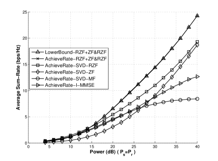
Figure 2: Average sum-rate versus the transmitting power with $P_{s}=P_{r}$, where $M_{b}=M_{r}=K=4$, and BS is at 0 point, RS is at 0.25 point, users are at 1.0 point

Fig. 2 shows the average sum-rate of the network versus the transmitting power, when all nodes positions are fixed. It is observed that the sum-rate offered by the proposed linear transmission strategy are higher than those by the other linear schemes at all SNR regime, when the RS is at position of a quarter of the distance from BS to users. Fig. 3 shows the average sum-rate of the network versus the RS’s position, when the powers at BS and RS are fixed. We can see that the average sum-rate of the proposed strategy is higher than those of the other linear schemes, when the RS is close to BS. From Fig. 4, the average sum rate gap between the proposed strategy and other linear schemes become larger when the number of antennas at BS and the number of users both increase simultaneously. From Fig. 2-4, it is clear that the proposed strategy outperforms other linear schemes without considering the DC in design, when the RS is close to BS. This is because that the BM schemes without considering DC in design cause $\mathrm{SINR}_{1k}$ loss (near to 0), which leads to rate loss when the channel gains of the DC and FC are considerable at the scenario that RS is close to BS. However, both SVD-RZF and SVD-ZF schemes outperform the proposed strategy when the RS is close to users, because: 1) the BC is bottleneck when the RS is close to users, and the FC is bottleneck when the RS is close to BS, vice versa, 2) the gain of BC by SVD surpasses the loss of the DC by SVD when the BC is bottleneck, and 3) the ZF receiving filter at RS will amplify the noise, especially at the case that the RS is close to users, which leads to rate loss of the proposed strategy.

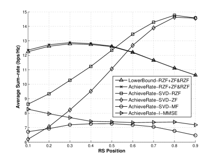
Figure 3: Average sum-rate versus RS position (between 0 and 1.0 ), where BS is at $0$ point and users are at $1.0$ point, $M_{b}=M_{r}=K=4$, and $P_{s}=P_{r}=28\mathrm{dB}$

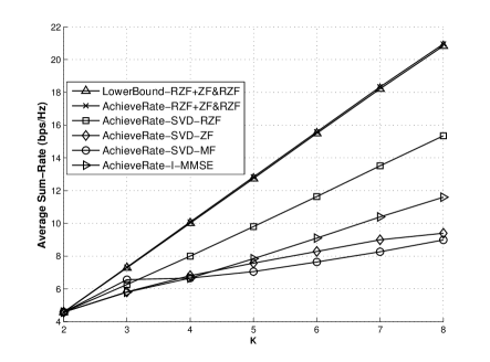
Figure 4: Average sum-rate versus $K$, where $K=M_{b}=M_{r}$, $P_{s}=P_{r}=28\mathrm{dB}$, and BS is at 0 point, RS is at 0.25 point, users are at 1.0 point.

VI Conclusion and discussions

In this letter, we propose a linear transmission strategy to design PM at BS and BM at RS for the MIMO relaying broadcast network with DC. In the proposed scheme, we take an RZF filter based on DC as the PM at BS, an RZF filter based on FC as transmitting BM at RS, and a ZF filter as receiving BM at RS based on the PM at BS and BC. Numerical results shown that the proposed strategy outperforms the other linear schemes without considering DC in design, when the RS is close to BS. In fact, the proposed linear strategy is a general scheme to design the PM at BS and BM at RS with DC. One can choose other linear precoders at BS and RS instead of the RZF, such as the precoder based on SLNR [11], and other relay linear receiving filter can be chosen as receiving BM at RS, such as MMSE [13] filter and so on.

References

• [1] C.-B. Chae, T. Tang, J. Robert W. Heath, and S. Cho, “MIMO relaying with linear processing for multiuser transmission in fixed relay networks,” IEEE Trans. Sig. Proc., vol. 56, no.2, FEB 2008.
• [2] R. Zhang, C. C. Chai, and Y.-C. Liang, “Joint beamforming and power control for multiantenna relay broadcast channel with QoS constraints,” IEEE Trans. Sig. Proc., vol. 57, no.2, pp. 726–737, Feb. 2009.
• [3] W. Xu, X. Dong, and W.-S. Lu, “Joint optimization for source and relay precoding under multiuser MIMO downlink channels,” in Proc. of the IEEE ICC 2010, June 2010.
• [4] W. Xu, X. Dong, and W.-S. Lu, “Joint precoding optimization for multiuser multi-antenna relaying downlinks using quadratic programming,” IEEE Trans. Commun., vol. 59, no.5, pp. 1228–1235, May 2011.
• [5] K. S. Gomadam and S. A. Jafar, “Duality of MIMO multiple access channel and broadcast channel with amplify-and-forward relays,” IEEE Trans. Commun., vol. 58, no.1, pp. 211–217, Jan 2010.
• [6] B. Zhang, Z. He, K. Niu, and L. Zhang, “Robust linear beamforming for MIMO relay broadcast channel with limited feedback,” IEEE Sign. Proc. Lett, vol. 17, no.2, pp. 209–212, Oct. 2010.
• [7] W. Xu, X. Dong, and W.-S. Lu, “MIMO relaying broadcast channels with linear precoding and quantized channel state information feedback,” IEEE Trans. Sig. Proc., vol. 58, no.10, pp. 5233–5245, Otc. 2010.
• [8] J. N. Laneman, D. Tse, and G. W. Wornell, “Cooperative diversity in wireless networks: Effcient protocols and outage behavior,” IEEE Trans. Inf. Theory, vol. 50, no.12, pp. 3062–3080, Dec 2004.
• [9] C. B. Peel, B. M. Hochwald, and A. L. Swindlehurst, “A vector-perturbation technique for near-capacity multiantenna multiuser communication-part I: Channel inversion and regularization,” IEEE Trans. Commun., vol. 53, no.1, pp. 195–202, Jan. 2005.
• [10] G. Caire and S. S. (Shitz), “On the achievable throughput of a multiantenna Gaussian broadcast channel,” IEEE Trans. Inf. Theory, vol. 49, no.7, pp. 1691–1706, July 2003.
• [11] M. Sadek, A. Tarighat, and A. H. Sayed, “A leakage-based precoding scheme for downlink multi-user MIMO channels,” IEEE Trans. Wireless Commun., vol. 6, no.5, May 2007.
• [12] X. Wang and X.-D. Zhang, “Linear transmission for rate optimization in MIMO broadcast channels,” IEEE Trans. Wireless Commun., vol. 9, no.10, Oct 2010.
• [13] D. Tse and P. Viswanath, Fundamentals of Wireless Communications. Cambridge University Press, 2005.
• [14] Z. Wang, W. Chen, and J. Li, “Efficient beamforming in MIMO relaying broadcast channels with imperfect channel estimations,” To appear in IEEE Trans. Veh. Tech.