Joint Source and Relay Design for Multi-user MIMO Non-regenerative Relay Networks with Direct Links

Abstract

In this paper, we investigate joint source precoding matrices and relay processing matrix design for multi-user multiple-input multiple-output (MU-MIMO) non-regenerative relay networks in the presence of the direct source-destination (S-D) links. We consider both capacity and mean-squared error (MSE) criterions subject to the distributed power constraints, which are nonconvex and apparently have no simple solutions. Therefore, we propose an optimal source precoding matrix structure based on the point-to-point MIMO channel technique, and a new relay processing matrix structure under the modified power constraint at relay node, based on which, a nested iterative algorithm of jointly optimizing sources precoding and relay processing is established. We show that the capacity based optimal source precoding matrices share the same structure with the MSE based ones. So does the optimal relay processing matrix. Simulation results demonstrate that the proposed algorithm outperforms the existing results.

I Introduction

Recently, MIMO relay network has attracted considerable interest from both academic and industrial communities. It has been verified that wireless relay can increase coverage and capacity of the wireless networks [1]. Meanwhile, MIMO techniques can provide significant improvement for the spectral efficiency and link reliability in scattered environments because of its multiplexing and diversity gains [2]. A MIMO relay network, combining the relaying and MIMO techniques, can make use of both advantages to increase the data rate in the network edge and extend the network coverage. It is a promising technique for the next generation’s wireless communications.

The capacity of MIMO relay network has been extensively investigated in the literature [3, 4, 5, 6, 7]. Recent works on MIMO non-regenerative relay are focusing on how to design the source precoding matrix and relay processing matrix. For a single-user MIMO relay network, an optimal relay processing matrix which maximizes the end-to-end mutual information is designed in [8] and [9] independently, and the optimal structures of jointly designed source precoding matrix and relay processing matrix are derived in [10]. In [11] and [12], the relay processing matrix to minimize the mean-squared error (MSE) at the destination is developed. A unified framework to jointly optimize the source precoding matrix and the relay processing matrix is established in [13]. For a multi-user single-antenna relay network, the optimal relay processing is designed to maximize the system capacity [14, 15, 16]. In [17], the optimal source precoding matrices and relay processing matrix are developed in the downlink and uplink scenarios of an MU-MIMO relay network without considering S-D links. There are only a few works considering the direct S-D links. In [18] and [19], the optimal relay processing matrix is designed based on MSE criterion with and without the optimal source precoding matrix in the presence of direct links, respectively. However, for a relay network with direct S-D links, jointly optimizing the source precoding matrix and the relay processing matrix based on capacity or MSE is much difficult, especially for an MU-MIMO relay network.

In this paper, we consider an MU-MIMO non-regenerative relay network where each node is equipped with multiple antennas. We take the effect of S-D link into the joint optimization of the source precoding matrices and relay processing matrix, which is more complicated than the relatively simple case without considering S-D links [17]. To our best knowledge, there is no such work in the literature on the joint optimization of source precoding and relay processing for MU-MIMO non-regenerative relay networks with direct S-D links. Two major contributions of this paper over the conventional works are as follows:

• We first introduce a general strategy to the joint design of source precoding matrices and relay processing matrix by transforming the network into a set of parallel scalar sub-systems just as a point-to-point MIMO channel under a relay modified power constraint, and show that the capacity based source precoding matrices and relay processing matrix respectively share the same structures with the MSE based ones.

• A nested iterative algorithm is presented to solve the joint optimization of sources precoding and relay processing based on capacity and MSE respectively. Simulation results show that the proposed algorithm outperforms the existing methods.

The rest of this paper is organized as follows. Section II illustrates the system model. Section III presents the optimal structures of source precoding and relay processing, and a nested iterative algorithm to solve the joint optimization of sources precoding and relay processing. Section IV devotes to the simulation results. Finally, Section V concludes the paper.

Notations: Lower-case letter, boldface lower-case letter, and boldface upper-case letter denote scalar, vector, and matrix, respectively. $\textsf{E}(\cdot)$, $\mathrm{tr}(\cdot)$, $(\cdot)^{-1}$, $(\cdot)^{{\dagger}}$, $|\cdot|$, and $\|\cdot\|_{F}$ denote expectation, trace, inverse, conjugate transpose, determinant, and Frobenius norm of a matrix, respectively. $\mathbf{I}_{N}$ stands for the identity matrix of order $N$. $\mathrm{diag}(a_{1},\ldots,a_{N})$ is a diagonal matrix with the $i$th diagonal entry $a_{i}$. $\log$ is of base $2$. $\mathcal{C}^{M\times N}$ represents the set of $M\times N$ matrices over complex field, and $\sim\mathcal{CN}(x,y)$ means satisfying a circularly symmetric complex Gaussian distribution with mean $x$ and covariance $y$. $[x]^{+}$ denotes $\max\{0,x\}$.

II System Model

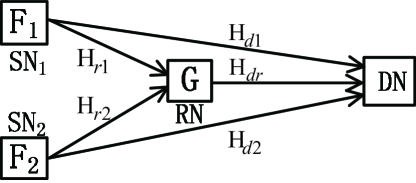
Figure 1: The multiple-access relay network with two source nodes, one relay node, and one destination node

We consider a multiple access MIMO relay network with two source nodes (SNs), one relay node (RN) and one destination node (DN) as illustrated in Fig. 1, where the channel matrices have been shown. The numbers of antennas equipped at the SNs, RN and DN are $N_{s},N_{r}$, and $N_{d}$, respectively. We assume that there is only two SNs and both SNs have the same number of antennas for simplicity. However, it is easy to be generalized to the scenario of multiple SNs with different numbers of antennas at each SN. In this paper, we consider a non-regenerative half-duplex relaying strategy applied at the RN to process the received signals. Thus, the transmission will take place in two phases. Suppose that perfect synchronization has been established between SN₁ and SN₂ prior to transmission, and both SN₁ and SN₂ transmit their independent messages to the RN and DN simultaneously during the first phase. Then the RN processes the received signals and forwards them to the DN during the second phase.

Let $\mathbf{H}_{ri}\in\mathcal{C}^{N_{r}\times N_{s}},\mathbf{H}_{di}\in\mathcal{C}^{N_{d}\times N_{s}},$ and $\mathbf{H}_{dr}\in\mathcal{C}^{N_{d}\times N_{r}}$ denote the channel matrices of the $i$th SN to RN, to DN, and RN to DN, respectively. Each entry of the channel matrices is assumed to be complex Gaussian variable with zero-mean and variance $\sigma^{2}_{h}$. Furthermore, all the channels involved are assumed to be quasi-static i.i.d. Rayleigh fading combining with large scale fading over a common narrow-band. Let $\mathbf{F}_{1}\in\mathcal{C}^{N_{s}\times N_{s}}$ and $\mathbf{F}_{2}\in\mathcal{C}^{N_{s}\times N_{s}}$ denote the precoding matrices for SN₁ and SN₂, respectively, which satisfy the power constraint $\textsf{E}[\mathbf{F}_{i}\mathbf{s}_{i}\mathbf{s}^{{\dagger}}_{i}\mathbf{F}^{{\dagger}}_{i}]=\mathrm{tr}(\mathbf{F}_{i}\mathbf{F}^{{\dagger}}_{i})\leq P_{i}$. Let $\mathbf{G}\in\mathcal{C}^{N_{r}\times N_{r}}$ denote the relay processing matrix. Suppose that $\mathbf{n}_{r}\in\mathcal{C}^{N_{r}\times 1}$ and $\mathbf{n}_{i}\in\mathcal{C}^{N_{d}\times 1}$ are the noise vectors at RN and DN, respectively, and all noise are independent and identically distributed additive white Gaussian noise (AWGN) with zero-mean and unit variance. Then, the baseband signal vectors $\mathbf{y}_{1}$ and $\mathbf{y}_{2}$ received at the DN during the two consecutive phases can be expressed as follows:

$$\underbrace{\left[\begin{array}[]{c}\mathbf{y}_{1}\\ \mathbf{y}_{2}\\ \end{array}\right]}_{\mathbf{Y}} = \underbrace{\left[\begin{array}[]{c}\mathbf{H}_{d1}\\ \mathbf{H}_{dr}\mathbf{G}\mathbf{H}_{r1}\end{array}\right]}_{\mathbf{H}_{1}}\mathbf{F}_{1}\mathbf{s}_{1}+\underbrace{\left[\begin{array}[]{c}\mathbf{H}_{d2}\\ \mathbf{H}_{dr}\mathbf{G}\mathbf{H}_{r2}\\ \end{array}\right]}_{\mathbf{H}_{2}}\mathbf{F}_{2}\mathbf{s}_{2}+$$ (13)

$$\underbrace{\left[\begin{array}[]{ccc}\mathbf{I}_{N_{d}}&\mathbf{0}&\mathbf{0}\\ \mathbf{0}&\mathbf{H}_{dr}\mathbf{G}&\mathbf{I}_{N_{d}}\\ \end{array}\right]}_{\mathbf{H}_{3}}\underbrace{\left[\begin{array}[]{c}\mathbf{n}_{1}\\ \mathbf{n}_{r}\\ \mathbf{n}_{2}\\ \end{array}\right]}_{\mathbf{N}},$$

where $\mathbf{s}_{i}\in\mathcal{C}^{N_{s}\times 1}$ is assumed to be a zero-mean circularly symmetric complex Gaussian signal vector transmitted by the $i$th SN and satisfies $\textsf{E}(\mathbf{s}_{i}\mathbf{s}^{{\dagger}}_{i})=\mathbf{I}_{N_{s}}$. Let Y, $\textbf{H}_{i}$ ($i=1,2,3$), and N, shown in (13), denote the effective receive signal, effective channels and effective noise respectively. Then $\mathbf{H}_{3}\textsf{E}[\mathbf{NN}^{{\dagger}}]\mathbf{H}_{3}^{{\dagger}}=\mathbf{H}_{3}\mathbf{H}_{3}^{{\dagger}}=\mathrm{diag}(\mathbf{I}_{N_{d}},\mathbf{R})$, where $\mathbf{R}=\mathbf{I}_{N_{d}}+\mathbf{H}_{dr}\mathbf{GG}^{{\dagger}}\mathbf{H}^{{\dagger}}_{dr}$ is the covariance matrix of the effective noise at the DN during the second phase.

III Optimal coordinates of Joint Source and Relay Design

In this section, the capacity and MSE for the MMSE detector with successive interference cancelation (SIC) at DN are analyzed. Then, we will exploit the optimal structures of source precoding and relay processing based on capacity and MSE respectively. Then a new algorithm on how to jointly optimize the sources precoding matrices and the relay processing matrix is proposed to maximize the capacity or minimize MSE of the entire network.

III-A Decoding Scheme

Conventional receivers such as matched filter (MF), zero-forcing (ZF), and MMSE decoder have been well studied in the previous works. The MF receiver has bad performance in the high SNR region, whereas the ZF produces a noise enhancement effect in the low SNR region. The MMSE detector with SIC has significant advantage over MF and ZF, which is information lossless and optimal [20]. Therefore, we consider the MMSE-SIC receiver at the DN and first decode the signal from SN₂ without loss of generality. With the predetermined decoding order, the interference from SN₂ to SN₁ is virtually absent. To exploit the optimal structures of the matrices at the SNs, we first set up the RN with a fixed processing matrix $\mathbf{G}$ without considering the power control. With the predetermined decoding order, the MMSE receive filter for SN_i ($i=1,2$) is given as [21][22]:

$$\mathbf{A}^{\mathrm{MMSE}}_{i}=\mathbf{F}^{{\dagger}}_{i}\mathbf{H}^{{\dagger}}_{i}(\mathbf{H}_{i}\mathbf{F}_{i}\mathbf{F}^{{\dagger}}_{i}\mathbf{H}^{{\dagger}}_{i}+\mathbf{R}_{Z_{i}})^{-1},$$ (14)

where $\mathbf{R}_{Z_{1}}\triangleq\mathbf{H}_{3}\mathbf{H}^{{\dagger}}_{3}~{}\mathrm{and}~{}\mathbf{R}_{Z_{2}}\triangleq\mathbf{H}_{3}\mathbf{H}^{{\dagger}}_{3}+\mathbf{H}_{1}\mathbf{F}_{1}\mathbf{F}^{{\dagger}}_{1}\mathbf{H}^{{\dagger}}_{1}.$ Then, the MSE-matrix for SN_i can be expressed as:

$$\mathbf{E}_{i} = \textsf{E}\left[(\mathbf{A}^{\mathrm{MMSE}}_{i}\mathbf{Y}_{i}-\mathbf{s}_{i})(\mathbf{A}^{\mathrm{MMSE}}_{i}\mathbf{Y}_{i}-\mathbf{s}_{i})^{{\dagger}}\right]$$ (15)

$$= \left(\mathbf{I}_{N_{s}}+\mathbf{F}^{{\dagger}}_{i}\mathbf{H}^{{\dagger}}_{i}\mathbf{R}^{-1}_{Z_{i}}\mathbf{H}_{i}\mathbf{F}_{i}\right)^{-1},$$

where $\mathbf{Y}_{1}=\mathbf{Y}-\mathbf{H}_{2}\mathbf{F}_{2}\mathbf{s}_{2}$ and $\mathbf{Y}_{2}=\mathbf{Y}$. Hence, the capacity for SN_i is given as [20]

$${C}_{i}=\log\left|\mathbf{I}_{N_{s}}+\mathbf{F}^{{\dagger}}_{i}\mathbf{H}^{{\dagger}}_{i}\mathbf{R}^{-1}_{Z_{i}}\mathbf{H}_{i}\mathbf{F}_{i}\right|=\log\left|\mathbf{E}^{-1}_{i}\right|.$$ (16)

III-B Optimal Precoding Matrices at SNs

In this subsection, we will introduce two lemmas, which will be used to exploit the optimal source precoding matrices and relay processing matrix, respectively.

Lemma 1

For a matrix $\mathbf{A}$, if matrix $\mathbf{B}$ is a positive definite matrix, and $\mathbf{C}=\mathbf{A}\mathbf{B}^{-1}\mathbf{A}^{{\dagger}}$, then $\mathbf{C}$ is an Hermitian and positive semidefinite matrix (HPSDM).

Proof:

Since $\mathbf{B}$ is a positive definite matrix, then $\mathbf{B}^{-1}$ is also a positive definite matrix. For any non-zero column vector x, let $\textbf{{y}}=\mathbf{A}^{{\dagger}}\textbf{{x}}$. Then we have $\textbf{{x}}^{{\dagger}}\mathbf{C}\textbf{{x}}=\textbf{{x}}^{{\dagger}}\mathbf{A}\mathbf{B}^{-1}\mathbf{A}^{{\dagger}}\textbf{{x}}=\textbf{{y}}^{{\dagger}}\mathbf{B}^{-1}\textbf{{y}}\geq 0$, which implies that $\mathbf{C}$ is an HPSDM. ∎

Lemma 2

If $\mathbf{A}$ and $\mathbf{B}$ are positive semidefinite matrices, then, $0\leq\mathrm{tr}(\mathbf{AB})\leq\mathrm{tr}(\mathbf{A})\mathrm{tr}(\mathbf{B})$, and, there is an $\alpha\in[0,1]$, such that $\mathrm{tr}(\mathbf{AB})=\alpha\mathrm{tr}(\mathbf{A})\mathrm{tr}(\mathbf{B})$.

Proof:

See [23, page 269]. ∎

Since $\mathbf{R}_{Z_{i}}~{}(i=1,2)$ is positive definite matrix [24], according to Lemma 1, $\mathbf{H}_{si}=\mathbf{H}^{{\dagger}}_{i}\mathbf{R}^{-1}_{Z_{i}}\mathbf{H}_{i}$ is HPSDM, which can be decomposed as:

$$\mathbf{H}_{si}=\mathbf{U}_{i}\mathbf{\Lambda}_{i}\mathbf{U}^{{\dagger}}_{i},$$ (17)

with unitary matrix $\mathbf{U}_{i}$, and non-negative diagonal matrices $\mathbf{\Lambda}_{i}$, which diagonal entries are in descending order. One of our main results of this paper is as below.

Propositon 1

For a given matrix $\mathbf{G}$ and predetermined decoding order, the precoding matrix for SN_i with the following canonical form

$$\mathbf{F}_{i}=\mathbf{U}_{i}\mathbf{\Sigma}_{i}~{}~{}(i=1,2)$$ (18)

is optimal with the water-filling power allocation policy (Policy-A) based on capacity or with the inverse water-filling power allocation policy (Policy-B) based on MSE, where:

$$\mathbf{\Sigma}^{2}_{i} = \left[\mu-\mathbf{\Lambda}^{-1}_{i}\right]^{+}~{}~{}~{}~{}~{}~{}~{}~{}~{}(\mathrm{Policy-A}),~{}~{}$$ (19a)

$$\mathbf{\Sigma}^{2}_{i} = \left[\mu\mathbf{\Lambda}^{-1/2}_{i}-\mathbf{\Lambda}^{-1}_{i}\right]^{+}~{}(\mathrm{Policy-B}),$$ (20a)

$$\mathrm{s.t} : \mathrm{tr}(\mathbf{\Sigma}^{2}_{i})=P_{i}.$$ (21a)

Proof:

Substituting $\mathbf{F}_{1}$ in (18) into (16) and (15), we respectively have:

$${C}_{1} = \log\left|\mathbf{I}_{N_{s}}+\mathbf{\Sigma}^{2}_{1}\mathbf{\Lambda}_{1}\right|,$$

$$\mathrm{tr}(\mathbf{E}_{1}) = \mathrm{tr}\left\{(\mathbf{I}_{N_{s}}+\mathbf{\Sigma}^{2}_{1}\mathbf{\Lambda}_{1})^{-1}\right\}.$$

According to KKT conditions [25], the Policy-A and Policy-B can make the capacity $C_{1}$ maximized and the MSE $\mathrm{tr}(\mathbf{E}_{1})$ minimized, respectively, under the power control $P_{1}$ at SN₁. This implies that $\mathbf{F}_{1}$ is optimal. After deciding $\mathbf{F}_{1}$, and substituting the $\mathbf{F}_{1}$ into $\mathbf{R}_{Z_{2}}$, we can prove that $\mathbf{F}_{2}$ is optimal. ∎

III-C A Nearly Optimal Processing Matrix at Relay

In this subsection, we first exploit the structure of relay processing matrix based on capacity for given $\mathbf{F}_{1}$ and $\mathbf{F}_{2}$. Then, we show that the same structure matrix at RN can make the MSE of the entire network near to minimum with a different power allocation policy. The capacity of the entire network is [20]

$$C=\log\left|\mathbf{H}_{1}\mathbf{\Pi}_{1}\mathbf{H}^{{\dagger}}_{1}+\mathbf{H}_{2}\mathbf{\Pi}_{2}\mathbf{H}^{{\dagger}}_{2}+\mathbf{H}_{3}\mathbf{H}^{{\dagger}}_{3}\right|-\log\left|\mathbf{H}_{3}\mathbf{H}^{{\dagger}}_{3}\right|,$$

where $\mathbf{\Pi}_{i}=\mathbf{F}_{i}\mathbf{F}^{{\dagger}}_{i}$. According to the determinant expansion formula of the block matrix [26], (III-C) can be rewritten as:

$$C = \log\left|\mathbf{T}\right|+\log\left|\mathbf{H}_{dr}\mathbf{G}\mathbf{K}\mathbf{G}^{{\dagger}}\mathbf{H}^{{\dagger}}_{dr}+\mathbf{R}\right|-\log\left|\mathbf{R}\right|,$$ (22)

where

$$\mathbf{T} = \mathbf{I}_{N_{d}}+\sum_{i=1}^{2}\mathbf{H}_{di}\mathbf{\Pi}_{i}\mathbf{H}^{{\dagger}}_{di},$$ (23a)

$$\mathbf{K} = \sum_{i=1}^{2}\mathbf{H}_{ri}\mathbf{\Pi}_{i}\mathbf{H}^{{\dagger}}_{ri}-\mathbf{\widetilde{K}},$$ (24a)

$$\mathbf{\widetilde{K}} = \left(\sum_{i=1}^{2}\mathbf{H}_{ri}\mathbf{\Pi}_{i}\mathbf{H}^{{\dagger}}_{di}\right)\mathbf{T}^{-1}\left(\sum_{i=1}^{2}\mathbf{H}_{di}\mathbf{\Pi}_{i}\mathbf{H}^{{\dagger}}_{ri}\right).$$ (25a)

Let $\Delta=\log|\mathbf{T}|$, which is independent of $\mathbf{G}$. Then, for given $\mathbf{F}_{1}$ and $\mathbf{F}_{2}$, the problem on maximum capacity of the network can be formulated as

$$\arg \max_{\mathbf{G}}~{}C=\log\left|\mathbf{H}_{dr}\mathbf{G}\mathbf{K}\mathbf{G}^{{\dagger}}\mathbf{H}^{{\dagger}}_{dr}+\mathbf{R}\right|-\log\left|\mathbf{R}\right|,$$ (26a)

$$\mathrm{s.t.} ~{}\mathrm{tr}\left\{\mathbf{G}\left(\mathbf{I}_{N_{r}}+\sum^{2}_{i=1}\mathbf{H}_{ri}\mathbf{\Pi}_{i}\mathbf{H}^{{\dagger}}_{ri}\right)\mathbf{G}^{{\dagger}}\right\}\leq P_{r}.$$ (27a)

To solve this problem, and find a nearly optimal processing matrix $\mathbf{G}$, due to $\mathbf{K}=\mathbf{K}^{{\dagger}}$, we first decompose $\mathbf{K}$ based on eigenvalue decomposition, and then decompose $\mathbf{H}_{dr}$ based on singular value decomposition, i.e.,

$$\mathbf{K} = \mathbf{U}_{K}\mathbf{\Lambda}_{K}\mathbf{U}^{{\dagger}}_{K},$$

$$\mathbf{H}_{dr} = \mathbf{U}_{H}\mathbf{\Theta}\mathbf{V}^{{\dagger}}_{H},$$

where $\mathbf{U}_{K},\mathbf{U}_{H}$ and $\mathbf{V}_{H}$ are unitary matrices, and $\mathbf{\Lambda}_{K}=\mathrm{diag}(\lambda_{1},\cdots,\lambda_{N_{r}})$ is an $N_{r}\times N_{r}$ diagonal matrix, and $\mathbf{\Theta}=\mathrm{diag}(\theta_{1},\cdots,\theta_{r})$ is an $N_{r}\times N_{r}$ diagonal matrix, which diagonal entries are in descending order.

From (26a), it is easy to verify that the optimal left canonical of $\mathbf{G}$ is still given by $\mathbf{V}_{H}$ [8]. But, it is intractable to find the optimal right canonical for the processing matrix $\mathbf{G}$, because there is no matrix which can achieve the diagonalization of both the capacity cost function (26a) and the power constraint (27a). But, we can modify the power constraint (27a) to another expression to find a matrix which has the desired property. Due to $\mathbf{K}$ is a deterministic matrix for the fixed sources precoding matrices, (27a) can be rewritten as

$$\mathrm{tr}\{\mathbf{G}(\mathbf{I}_{N_{r}}+\mathbf{K})\mathbf{G}^{{\dagger}}\}+\mathrm{tr}\{\mathbf{\widetilde{K}}\mathbf{G}^{{\dagger}}\mathbf{G}\}=\\ \mathrm{tr}\left\{\mathbf{G}\left(\mathbf{I}_{N_{r}}+\sum^{2}_{i=1}\mathbf{H}_{ri}\mathbf{\Pi}_{i}\mathbf{H}^{{\dagger}}_{ri}\right)\mathbf{G}^{{\dagger}}\right\}\leq P_{r}.$$ (28)

Since $\mathbf{T}$ is a positive definite matrix, according to Lemma 1, $\mathbf{\widetilde{K}}$ in (25a) is also a positive semidefinite matrix. According to Lemma 2, the new power constraint at the RN can be expressed as

$$\mathrm{tr}\{\mathbf{G}(\mathbf{I}_{N_{r}}+\mathbf{K})\mathbf{G}^{{\dagger}}\}+\alpha\mathrm{tr}\{\mathbf{\widetilde{K}}\}\mathrm{tr}\{\mathbf{G}^{{\dagger}}\mathbf{G}\}\approx\\ \mathrm{tr}\left\{\mathbf{G}(\mathbf{I}_{N_{r}}+\sum^{2}_{i=1}\mathbf{H}_{ri}\mathbf{F}_{i}\mathbf{F}^{{\dagger}}_{i}\mathbf{H}^{{\dagger}}_{ri})\mathbf{G}^{{\dagger}}\right\}\leq P_{r},$$ (29)

where the exact value $\alpha$ can be found by an iterative method. Thus, applying the results in [8][17], the processing matrix $\mathbf{G}$ with the following structure can achieve the desired diagonalization for both capacity cost function (26a) and the new power constraint (29), and will be optimal [8]:

$$\mathbf{G}=\mathbf{V}_{H}\mathbf{\Xi}\mathbf{U}^{{\dagger}}_{K},$$ (30)

where $\mathbf{\Xi}^{2}=\mathrm{diag}(\xi_{1},\cdots,\xi_{N_{r}})$ can be solved by optimization method [8].

Let $\kappa=\mathrm{tr}\{\mathbf{\widetilde{K}}\}$. Substituting $\mathbf{G}$ into (26a), and using the new power constraint (29) to replace (27a), the problem (26a) to find $\xi_{i}$ becomes

$$\arg \max_{\xi_{1},~{}\ldots,~{}\xi_{N_{r}}}~{}C(\xi_{i})=\sum^{N_{r}}_{i=1}\log\frac{\theta^{2}_{i}\xi_{i}\lambda_{i}+\theta^{2}_{i}\xi_{i}+1}{\theta^{2}_{i}\xi_{i}+1},$$ (31a)

$$\mathrm{s.t.} ~{}\sum^{N_{r}}_{i=1}(\lambda_{i}+\alpha\kappa+1)\xi_{i}\leq P_{r}~{}~{}\mathrm{and}~{}~{}\xi_{i}\geq 0,~{}\forall i~{}.$$ (32a)

Then, this optimization problem with respect to $\xi_{i}$ is similar to a problem solved in [8, 17]. Then we have

$$\xi_{i}=\frac{1}{2\theta^{2}_{i}(\lambda_{i}+1)}\left[\sqrt{\lambda^{2}_{i}+\frac{4\lambda_{i}\theta^{2}_{i}(\lambda_{i}+1)\mu}{\lambda_{i}+1+\alpha\kappa}}-\lambda_{i}-2\right]^{+}$$ (33)

$$\sum^{N_{r}}_{i=1}(\lambda_{i}+1+\alpha\kappa)\xi_{i}\leq P_{r}.$$ (34)

where $\mu$ in (33) is decided by (34).

Next, we will show that the same structure matrix $\mathbf{G}$ can also make the MSE of the entire network near to minimum with a different power allocation matrix $\mathbf{\Xi}$ for given $\mathbf{F}_{1}$ and $\mathbf{F}_{2}$. Due to the total MSE can be expressed as:

$$J(\mathbf{G}) = \mathrm{tr}(\mathbf{E}_{1})+\mathrm{tr}(\mathbf{E}_{2})$$ (35)

$$\overset{a}{\leq} \mathrm{tr}(\mathbf{\tilde{E}}_{1})+\mathrm{tr}(\mathbf{E}_{2})$$

$$= \mathrm{tr}\left\{(\mathbf{I}_{2N_{d}}+\mathbf{F}^{{\dagger}}\mathbf{H}^{{\dagger}}\mathbf{R}^{-1}_{Z_{1}}\mathbf{H}\mathbf{F})^{-1}\right\}$$

$$\overset{b}{=} \mathrm{tr}(\mathbf{I}_{2N_{d}})-\mathrm{tr}\left\{(\mathbf{R}_{Z_{1}}+\mathbf{H}\mathbf{F}\mathbf{F}^{{\dagger}}\mathbf{H}^{{\dagger}})^{-1}\mathbf{H}\mathbf{F}\mathbf{F}^{{\dagger}}\mathbf{H}^{{\dagger}}\right\}$$

$$= \mathrm{tr}\left\{(\mathbf{R}_{Z_{1}}+\mathbf{H}\mathbf{F}\mathbf{F}^{{\dagger}}\mathbf{H}^{{\dagger}})^{-1}\mathbf{R}_{Z_{1}}\right\}$$

$$\overset{c}{=} \beta\mathrm{tr}\left\{(\mathbf{H}_{dr}\mathbf{G}\mathbf{K}\mathbf{G}^{{\dagger}}\mathbf{H}^{{\dagger}}_{dr}+\mathbf{R})^{-1}\right\}\mathrm{tr}\left\{(\mathbf{I}_{N_{d}}+\mathbf{R})\right\}$$

$$\triangleq \beta\tilde{J}(\mathbf{G}),$$

where $\mathbf{F}=\mathrm{diag}(\mathbf{F}_{1},\mathbf{F}_{2})$, $\mathbf{H}=[\mathbf{H}_{1}~{}\mathbf{H}_{2}]$, $\beta$ is a scalar factor. In (35), (a) come from the fact that noise is enhanced by using $\mathbf{\tilde{R}}_{Z_{1}}=\mathbf{H}_{3}\mathbf{H}^{{\dagger}}_{3}+\mathbf{H}_{2}\mathbf{\Pi}_{2}\mathbf{H}^{{\dagger}}_{2}$ to replace $\mathbf{R}_{Z_{1}}$ in calculating $\mathrm{tr}(\mathbf{\tilde{E}}_{1})$, (b) follows from Woodbury identity and $\mathrm{tr}(\mathbf{AB})=\mathrm{tr}(\mathbf{BA})$, and (c) follows from Lemma 2 and Schur complement to inverse a block matrix [26]. From (35), to minimize the $J(\mathbf{G})$ is equivalent to minimize $\tilde{J}(\mathbf{G})$. Then, for given $\mathbf{F}_{1}$ and $\mathbf{F}_{2}$, the optimal $\mathbf{G}$ to minimize MSE is

$$\arg ~{}\min_{\mathbf{G}}~{}\tilde{J}(\mathbf{G}),$$ (36a)

$$\mathrm{s.t.} :~{}~{}~{}~{}(\ref{eq:NewPowerConstr}).$$ (37a)

From the analysis above, the structure of $\mathbf{G}$ in (30) can also achieve the diagonalization of the equation (36a), but, has a new power allocation matrix $\mathbf{\Xi}$ different from that of capacity based one. Then, substituting $\mathbf{G}$ in (30) into (36a) to find the new $\mathbf{\Xi}$, (36a) becomes

$$\arg \min_{\xi_{1},\ldots,~{}\xi_{N_{r}}}\tilde{J}(\xi_{i}),$$ (38a)

$$\mathrm{s.t.} :~{}~{}(\ref{eq:NewPower-R}).$$ (39a)

where

$$\tilde{J}(\xi_{i})=\left(\sum\limits^{N_{r}}_{i=1}\left(\theta^{2}_{i}\lambda_{i}\xi_{i}+\theta^{2}_{i}\xi_{i}+1\right)^{-1}\right)\left(\sum\limits^{N_{r}}_{i=1}(\theta^{2}_{i}\xi_{i}+2)\right).$$

This problem can be solved by numerical optimization methods [25].

III-D Iterative Algorithm

In the above discussion, with predetermined decoding order and fixed $\mathbf{G}$, $\mathbf{F}_{1}$ and $\mathbf{F}_{2}$ can be optimized; For $\mathbf{F}_{1}$ and $\mathbf{F}_{2}$, $\mathbf{G}$ can be optimized. Therefore, we propose an iterative algorithm to jointly optimize $\mathbf{F}_{1},\mathbf{F}_{2}$ and $\mathbf{G}$ based on capacity. Note that, the MSE based algorithm can be easily obtained as well. The convergence analysis of the proposed iterative algorithm is intractable. But, it can yield much better performance than the existing methods, which will be demonstrated by the simulation results in the next section.

In summary, we outline the nested iterative algorithm as follows:

Algorithm 1 : A nested iterative algorithm.

  ${\bullet}$ Initialization: $\mathbf{G}$.

  ${\bullet}$ Repeat: Update $k:=k+1$;

     – Compute $\mathbf{F}^{(k)}_{1}$ based on $\mathbf{G}^{(k)}$;

     – Compute $\mathbf{F}^{(k)}_{2}$ based on $\mathbf{G}^{(k)}$ and $\mathbf{F}^{(k)}_{1}$;

     – Compute $\mathbf{G}^{(k+1)}=\mathbf{V}_{H}\mathbf{\Xi}\mathbf{U}_{K}$ based on $\mathbf{F}^{(k)}_{1}$ and $\mathbf{F}^{(k)}_{2}$ by the following inner repeat to find $\mathbf{\Xi}$;

${\circ}$  Initial: $\alpha$;

${\circ}$  Inner Repeat : Update $n:=n+1$;

    – Compute $\mathbf{\Xi}^{(n)}$ based on $\alpha^{(n)}$;

    – Compute $\alpha^{(n+1)}$ based on $\mathbf{\Xi}^{(n)}$;

${\circ}$ Inner Until: Convergence.

  $\bullet$ Until: The termination criterion is satisfied.

IV Simulation Results

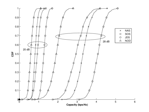
Figure 2: CDF of the capacity for different power constraints, $P_{1}=P_{2}=P_{r}=20\mathrm{dB}$ and  $P_{1}=P_{2}=P_{r}=28\mathrm{dB}$, $N_{s}=N_{r}=N_{d}=4$, $\ell_{sd}=10,~{}\ell_{sr}=\ell_{rd}=5$

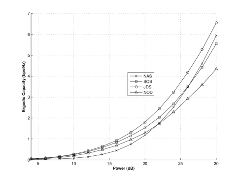
Figure 3: The capacity versus the power constraints $P_{i}~{}(i=1,2,r)$ (dB), $P_{1}=P_{2}=P_{r}$, and $N_{s}=N_{r}=N_{d}=4$, $\ell_{sd}=10,~{}\ell_{sr}=\ell_{rd}=5$.

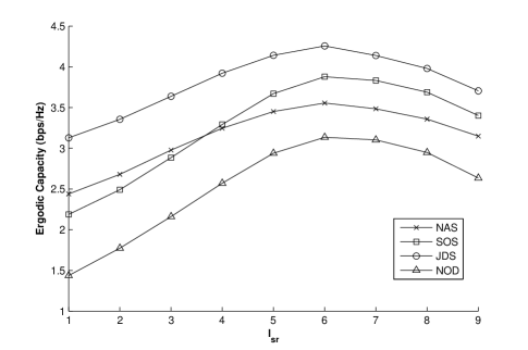
Figure 4: The capacity versus the distance between source-to-relay ($\ell_{sr})$,  $\ell_{sd}=10,~{}\ell_{rd}=\ell_{sd}-\ell_{sr}$, and $P_{1}=P_{2}=P_{r}=26\mathrm{dB}$, $N_{s}=N_{r}=N_{d}=4$.

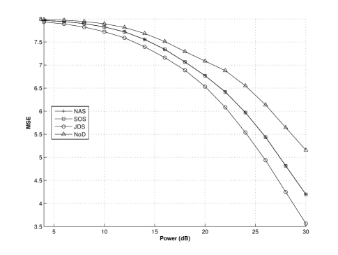
Figure 5: The sum-MSE versus the power constraints $P_{i}~{}(i=1,2,r)$ (dB), $P_{1}=P_{2}=P_{r}$, and $N_{s}=N_{r}=N_{d}=4$, $\ell_{sd}=10,~{}\ell_{sr}=\ell_{rd}=5$.

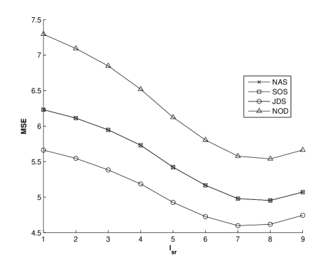
Figure 6: The sum-MSE versus the distance between source-to-relay ($\ell_{sr})$,  $\ell_{sd}=10,~{}\ell_{rd}=\ell_{sd}-\ell_{sr}$, and $P_{1}=P_{2}=P_{r}=26\mathrm{dB}$, $N_{s}=N_{r}=N_{d}=4$.

In this section, simulation results are carried out to verify the performance superiority of the proposed joint source-relay design scheme (JDS) for MU-MIMO relay network with direct links. We first compare the proposed scheme with other three schemes in terms of the ergodic capacity and the Cumulative Distribution Function (CDF) of instantaneous capacity of the MIMO relaying networks, and then compare the sum-MSE of the networks. The alternative schemes are:

1. Naive scheme (NAS): The source covariances are fixed to be scaled by the identity matrices $\frac{P_{1}}{N_{S}}\mathbf{I}$ and $\frac{P_{2}}{N_{S}}\mathbf{I}$ at SN₁ and SN₂, respectively, and the relay processing matrix is $\mathbf{G}=\eta\mathbf{I}$, where $\eta=\sqrt{\frac{P_{r}}{\mathrm{tr}(\mathbf{I}+\sum^{2}_{i=1}\mathbf{H}_{ri}\mathbf{F}_{i}\mathbf{F}^{{\dagger}}_{i}\mathbf{H}^{{\dagger}}_{ri})}}$ is a power control factor. The S-D links contribution is included.

2. Suboptimal scheme (SOS): This scheme is proposed in [17] for MU-MIMO relay network without considering S-D links in design. But, the S-D links contribution of capacity is included in the simulation for fair comparison. Note that this scheme is optimal for the scenario without considering the S-D links.

3. No-direct links scheme (NOD): This scheme is like SOS, but, without S-D links contribution.

Noting that both SOS and NOD have different power control polices to accommodate the capacity and MSE criterions. In the simulations, we consider a linear two-dimensional symmetric network geometry as depicted in Fig. 1, where both SNs are deployed at the same position, and the distance between SNs (or RN) and DN is set to be $\ell_{sd}$ (or $\ell_{rd}$), and $\ell_{sd}=\ell_{sr}+\ell_{rd}$. The channel gains are modeled as the combination of large scale fading (related to distance) and small scale fading (Rayleigh fading), and all channel matrices have i.i.d. $\mathcal{CN}(0,\frac{1}{\ell^{\tau}})$ entries, where $\ell$ is the distance between two nodes, and $\tau=3$ is the path loss exponent.

Fig. 2-4 are based on capacity criterion. Fig. 2 shows the CDF of instantaneous capacity for different power constraints, when all nodes positions are fixed. Fig. 3 shows the capacity of the network versus the power constraints, when all nodes positions are fixed. These two figures show that capacity offered by the proposed relaying scheme is better than both SOS and NOD schemes at all SNR regime, especially at high SNR regime. The naive scheme surpasses both SOS and NOD schemes at high SNR regime, which demonstrates that the direct S-D link should not be ignored in design. Fig. 4 shows the capacity of the network versus the distance ($\ell_{sr}$) between SNs and RN, for fixed $\ell_{sd}$. It is clear that the capacity offered by the proposed scheme is better than those by the SOS, NAS and NOD schemes. NOD scheme is the worst performance scheme at any relay position at moderate and high SNR regimes.

Fig. 5 and Fig. 6, are based on MSE criterion, the similar conclusions can be drawn.

V Conclusion

In this paper, we propose a optimal structure of the source precoding matrices and relay processing matrix for MU-MIMO non-regenerative relay network with direct S-D links based on capacity and MSE respectively. We show that the capacity based optimal source precoding matrices share the same structures with the MSE based ones. So does relay processing matrix. A nested iterative algorithm jointly optimizing the source precoding and relay processing is proposed. Simulation results show that the proposed algorithm provides better performance than the existing methods.

References

• [1] R. Pabst, B. H. Walke, D. C. Schultz, S. Mukherjee, H. Viswanathan, D. D. Falconer, and G. P. Fettweis, “Relay-based deployment concepts for wireless and mobile broadband radio,” IEEE Commun. Mag., vol. 42, no.9, pp. 80–89, Sept 2004.
• [2] L. Zheng and D. N. Tse, “Diversity and multiplexing: A fundamental tradeoff in multiple antenna channels,” IEEE Trans. Inf. Theory, vol. 8, no.1, pp. 2–25, August 2002.
• [3] B. Wang, J. Zhang, and A. Høst-Madsen, “On the capacity of MIMO relay channels,” IEEE Trans. Inf. Theory, vol. 51, no.1, pp. 29–43, Jan. 2005.
• [4] Z. Wang, W. Chen, F. Gao, and J. Li, “Capacity performance of relay beamformings for MIMO multirelay networks with imperfect $\mathcal{R}$-$\mathcal{D}$ CSI at relays,” IEEE Trans. Veh. Tech., vol. 60, no.6, pp. 2608–2619, July 2011.
• [5] C. K. Lo, S. Vishwanath, and J. Robert W. Heath, “Rate bounds for MIMO relay channels using precoding,” in Proc. of the IEEE GLOBECOM 2005, St.Louis, MO, vol. 3, pp. 1172–1176, Nov. 2005.
• [6] H. Bölcskei, R. U. Nabar, Özgür Oyman, and A. J. Paulraj, “Capacity scaling laws in MIMO relay networks,” IEEE Trans. Inf. Theory, vol. 5, no.6, pp. 1143–1444, Jun. 2006.
• [7] H. Wan, W. Chen, and J. Ji, “Efficient linear transmission strategy for mimo relaying broadcast channels with direct links,” IEEE Wireless Commun. Lett., vol. 1, pp. 14–17, Feb. 2012.
• [8] X. Tang and Y. Hua, “Optimal design of non-regenerative MIMO wireless relays,” IEEE Trans. Wireless Commun., vol. 6, no.4, pp. 1398–1407, Apr. 2007.
• [9] O. M. noz Medina, J. Vidal, and A. Agustín, “Linear transceiver design in nonregenerative relays with channel state information,” IEEE Trans. Sig. Proc., vol. 55, no.6, pp. 2593–2604, Jun. 2007.
• [10] Z. Fang, Y. Hua, and J. C. Koshy, “Joint source and relay optimization for a non-regenerative MIMO relay,” in Proc. of the IEEE Workshop Sensor Array Multi-Channel Processing, Waltham, MA, 2006.
• [11] W. Guan and H. Luo, “Joint MMSE transceiver design in non-regenerative MIMO relays systems,” IEEE Commun. Lett., vol. 55, no.12, pp. 517–519, July. 2008.
• [12] A. S. Behbahani, R. Merched, and A. M. Eltawil, “Optimizations of a MIMO relay network,” IEEE Trans. Sig. Proc., vol. 56, no.10, pp. 5062–5073, Oct. 2008.
• [13] Y. Rong, X. Tang, and Y. Hua, “A unified framework for optimizing linear nonregenerative multicarrier MIMO relay communication systems,” IEEE Trans. Sig. Proc., vol. 57, no.12, pp. 4837–4851, Dec. 2009.
• [14] L. Weng and R. D. Murch, “Multi-user MIMO relay system with self-interference cancellation,” in Proc. of the IEEE Wireless Communications Networking Conf.(WCNC), pp. 958–962, 2007.
• [15] C.-B. Chae, T. Tang, J. Robert W. Heath, and S. Cho, “MIMO relaying with linear processing for multiuser transmission in fixed relay networks,” IEEE Trans. Sig. Proc., vol. 56, no.2, FEB 2008.
• [16] K. S. Gomadam and S. A. Jafar, “Duality of MIMO multiple access channel and broadcast channel with amplify-and-forward relays,” IEEE Trans. Commun., vol. 58, no.1, pp. 211–217, Jan 2010.
• [17] Y. Yu and Y. Hua, “Power allocation for a MIMO relay system with multiple-antenna users,” IEEE Trans. Sig. Proc., vol. 58, no.5, pp. 2823–2835, May 2010.
• [18] Y. Rong and F. Gao, “Optimal beamforming for non-regenerative MIMO relays with direct link,” IEEE Commun. Lett., vol. 13, no.12, pp. 926–928, Dec. 2009.
• [19] Y. Rong, “Optimal joint source and relay beamforming for MIMO relays with direct link,” IEEE Commun. Lett., vol. 14, no.5, pp. 390–392, May. 2010.
• [20] D. Tse and P. Viswanath, Fundamentals of Wireless Communications. Cambridge University Press, 2005.
• [21] S. M.Kay, Fundamental of Statistical Signal Processing: Estimation Theory. EngLewood Cilffs, NJ: Prentice Hall, 1993.
• [22] S. S. Christensen, R. agarwal, E. de Carvalho, and J. M.Cioffi, “Weighted sum-rate maximization using weighted MMSE for MIMO-BC beamforming design,” IEEE Trans. Wireless Commun., vol. 7, no.12, Dec. 2008.
• [23] E. H. Lieb and W. Thirring, Studies in Mathematical Physics, Essays in Honor of Valentine Bartmann. Princeton University Press, Princeton, NJ, USA,, 1976.
• [24] M. H.Hayes, Statistical Digital Signal Processing and Modeling. John Wiley & Sons, Inc., 1996.
• [25] S. Boyd and L. Vandenberghe, Convex Optimization. Cambridge University Press, 2004.
• [26] R. A. Horn and C. R. Johnson, Topics in Matrix Analysis. Cambridge University Press, 1991.