Using machine learning to speed up new and upgrade detector studies: a calorimeter case

Abstract

In this paper, we discuss the way advanced machine learning techniques allow physicists to perform in-depth studies of the realistic operating modes of the detectors during the stage of their design. Proposed approach can be applied to both design concept (CDR) and technical design (TDR) phases of future detectors and existing detectors if upgraded. The machine learning approaches may speed up the verification of the possible detector configurations and will automate the entire detector R&D, which is often accompanied by a large number of scattered studies. We present the approach of using machine learning for detector R&D and its optimisation cycle with an emphasis on the project of the electromagnetic calorimeter upgrade for the LHCb detectorlhcls3 . The spatial reconstruction and time of arrival properties for the electromagnetic calorimeter were demonstrated.

1 Introduction

The calorimeters are an essential part of most of the existing and developing detectors in high energy physics. The high luminosity delivered by the collider causes a high multiplicity and hit occupancy in the calorimeter. In order to operate under such conditions a new generation of the calorimeters is characterised by high granularity (increased number of channels) and by the ability to measure the time of arrival of the particles to mitigate pile-up.

To obtain the planned physical performance during the R&D of modern experiments in HEP, the detailed Geant4 simulationgeant4 of the calorimeter is necessary. Such simulations are computationally expensive taking into account the large number of channels and the variety of possible options in the calorimeter module technologies, in the modules arrangement, in the reconstruction of the attributes of physical objects, etc. The optimisation cycle, within the calorimeter R&D, comprises several computationally intensive elements, such as shower development and particle transport. Processes of multi-parametric optimisation appear to be also expensive. These factors make new approaches to calorimeter development necessary. Machine learning allows a quick turnover for the optimisation cycle, when parameters are changed, and eliminates manual work for re-tuning the simulation and reconstruction.

2 Spatial Reconstruction

To reconstruct the hit position of the particle reached calorimeter, we implement an approach which is based on Pythia8-generated events of $B_{s}^{0}\rightarrow J/\psi(\rightarrow\mu^{+}\mu^{-})\pi^{0}(\rightarrow\gamma\gamma)$ (hereinafter signal sample), generated with default LHCb tunings and on a data of Geant4-simulated events in the simplified high-granularity detector. This simplified simulation setup uses the same alternating layers of scintillator and lead plates (Shashlik technology), as in LHCb Electromagnetic calorimeter (ECAL)lhcbmain and it consists of a matrix of 30x30 cells of size 20.2x20.2 mm² in $\eta$ – $\phi$ plane. This allows us to emulate each type of current ECAL modules: inner, middle or outer with cells size of 40.4x40.4 mm², 60.6x60.6 mm² or 121.2x121.2 mm², respectively.

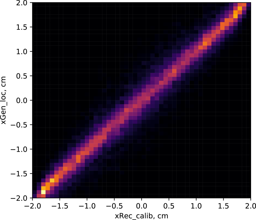
For each photon from the signal sample, we find the closest track in Geant4 simulated data. The calorimeter cell, in which the signal produces the hit is required to be surrounded by two layers of cells of the same type. Thus, a matrix of 5x5 cells of the same type is obtained. We suppose that most of the clusters of the signal sample do not exceed the size of such a matrix. Inside this matrix, the cell with the highest energy deposit is searched. The barycentre of the cluster is the reconstructed position of the photon which released energy in the calorimeter. The dependence of each of the local coordinates of the signal cluster barycentre on the corresponding true coordinate of the hit position we call the S-curve due to its distinctive shape. The S-curves of both x and y coordinates for the inner region are displayed in Figure 1. The difference between the S-curve and the straight line characterises the quality of spatial reconstruction. Several approaches were tested to calibrate the S-curve (hit position reconstruction): the parametric approach and the machine learning approach using XGBoost regressorxgboost . The results of the calibration for these approaches are shown in Figure 2 and in Table 1.

Figure 1: The dependence (2-dimensional distribution) of local coordinates of signal cluster barycentre on true coordinates of the hit position for inner modules. The local coordinates are of x (left) and y (right). Here and in the Figure 2 colour from violet (dark) to yellow (bright) represents the normalised counts of the events from 0.0 to 1.0, respectively.

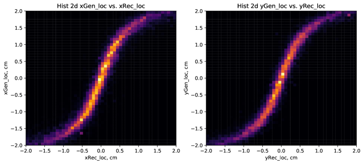
As a metric of spatial resolution we use RMSE of the difference between true and reconstructed local coordinate (independent of x and y) of the hit. The observed difference in the metric, based on local coordinates x and y was found to be negligible. Therefore, all the results exploited in this metric are presented for local coordinate x.

Figure 2: S-curve calibration results for inner modules and local coordinate x using parametric approach (left) and XGBoost regressor (right).

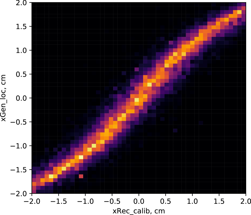
For the parametric approach, the reconstructed local coordinate x is represented as ${a\cdot arcsinh(b\cdot x)}$. The parameters for the calibration were found using random searchrandom with 1000² points in the range (0.01, 100) for each parameter. The best parameters obtained using a parametric approach for the inner section are: a = 1.15, b = 2.07.

The selected machine learning approach was based on the extreme gradient boosting (XGBoost), and among its hyperparameters colsample_bytree, gamma, max_depth and min_child_weight were selected, which are typical for such a problem. These hyperparameters were optimised using BayesSearchCV, within the ranges (1, 20), (1, 10), (0.1, 0.9) and (0.3, 0.7), respectively. The chosen parameters colsample_bytree = 0.7, gamma = 0.1, max_depth = 20, min_child_weight = 10 (the set of values is for the inner section) provide best results without overtraining being observed. As a result, we used 5-fold cross-validation and trained the regressor using 30% events of the sample.

ECAL region	Inner	Middle	Outer
Uncalibrated	0.860 $\pm$ 0.007	1.413 $\pm$ 0.017	3.795 $\pm$ 0.030
Calibration
Parametric	0.522 $\pm$ 0.009	0.964 $\pm$ 0.012	2.780 $\pm$ 0.025
XGBoost	0.117 $\pm$ 0.002	0.267 $\pm$ 0.004	0.731 $\pm$ 0.002

Table 1: Spatial reconstruction results (RMSE, cm) of local coordinate x for uncalibrated data, and for the data calibrated using parametric approach and XGBoost regressor.

3 Pile-up Mitigation with Timing

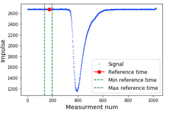
Among the requirements for the LHCb Phase 2 Upgrade ECAL, is the ability to measure the time of arrival of the photon or electron with an accuracy of few tenths of a picosecond. The difficulty is that the time-of-arrival properties are hard to reproduce in an accurate simulation. We used test beam results to evaluate important simulation parameters, as well as calibrate simulation on points measured during the test beam. The data was obtained from the electron test beam and consists of 7848 signals, where each signal contain 1024 impulse measurements sampled with a step of 200 picoseconds (5 GHz) involving the reference time of the signal. The time of arrival has been studied in two cases: single signal and two overlapped signals. The goal of using machine learning algorithms is to evaluate limitations of the possible physics performance driven by test beam data.

3.1 Single signal

In the case of a single signal, the machine learning algorithms were used to evaluate its reference time. It has been investigated how accurately the reference time can be reconstructed depending on the sampling rates. The second case is based on reference time reconstruction, in the presence of the second signal. Additionally, machine learning was applied for the classification in which cases the data contain one signal, or multiple ones.

The raw signal obtained during the test beam, is presented in Figure 3 (left). Artificial re-sampling allows us to reduce data while retaining the signal shape as shown in Figure 3 (right).

Figure 3: Signal sampling before (left) and after dimensionality reduction (right).

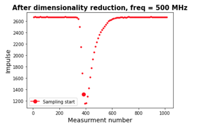
The procedure of test beam data analysis starts with the choosing of an initial sampling point. Afterwards, given a frequency k, each k-th point was sampled towards both lower and higher frequencies.

Figure 4: Models comparison for time difference RMSE (ns) w.r.t. sampling frequency (MHz).

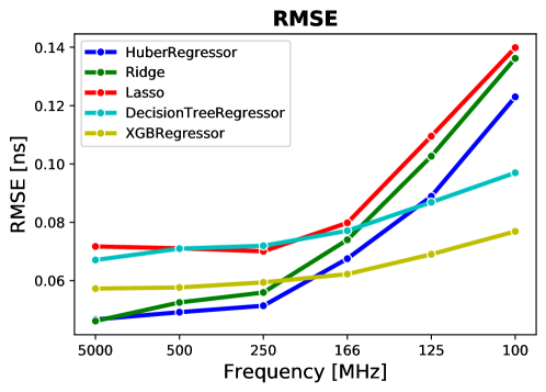
The reference time was predicted using 5 different models. All the regressors have been tuned using Bayesian optimisation. Feature engineering for the selected regressors did not show any significant improvement in the results. Time difference RMSE was chosen as a loss function. The comparison of 5 selected models is shown in Figure 4. Different regressors demonstrate similar results. One can see that the sampling frequency can be reduced from 5 GHz to 250 MHz without considerable changes of time reconstruction. Subsequent results were obtained using the XGBoost regressorxgboost .

3.2 Overlapping signals

High pile-up conditions imply overlap of signals from different vertices. Timing information can be used to mitigate pile-up. Hereinafter, we consider signal processing at the readout for an individual calorimeter cell.

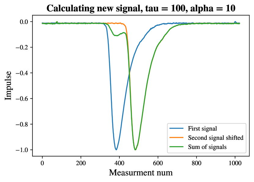
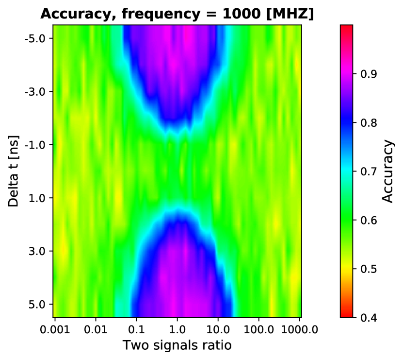
Since we didn’t have samples with multiple signals, we generated it under given amplitude ratio and time shift. The resulted signal can be parameterised as $S_{\mathrm{res}}=S_{1}+\alpha\cdot{}S_{2}^{\mathrm{shifted}}$, where $S_{1}$ and $S_{2}$ are different signals obtained from the test beam data in the same way as described in Section 3.1. The reference time of the signal which amplitude is greater is assigned to the reference time of the resulting signal. Figure 5 (left) shows the generated signal. By aggregation of the arrival time difference ($\tau$) and ratio ($\alpha$) of two signals one can produce 2-dimensional distributions over these variables as displayed in Figure 5 (right). It demonstrates the accuracy of our predictions on these two parameters for two different datasets.

Figure 5: Generated and initial signals (left). The 2-dimensional distribution of arrival time difference and signal ratio of two signals for sampling frequency 1000 MHz (right).

3.3 Reference time prediction in the presence of the second signal

The final model for time difference/amplitude separation of two signals employs an ensemble of models of KNeighborsClassifier, DecisionTreeClassifier and RandomForestClassifier. The models were tuned using Bayesian optimisation separately for each sampling frequency. A variety of strategies we tried for probabilistic class estimation, such as âlinearâ, âharmonicâ, âgeometricâ and ârank averagingâ. âHarmonicâ resulted as the best one according to the cross-validation.

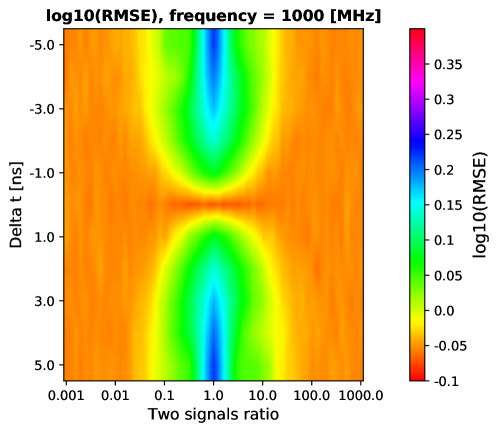
Figure 6 demonstrates the ability of the final model to evaluate time reconstruction in the presence of the second signal.

Figure 6: The 2-dimensional distribution of arrival time difference and signal ratio of two signals for sampling frequency 1000 MHz.

4 Conclusion

The proposed approaches of spatial reconstruction and time of arrival properties of the LHCb electromagnetic calorimeter illustrate the idea of automation of the detector development and its optimisation cycle. The results obtained, using the discussed approaches, addresses physics performance aspects which are known to be computationally expensive for accurate simulation. The spatial reconstruction using both parametric and machine learning approaches was obtained. The performance of the selected XGBoost configuration surpass those of the parametric approach for each of calorimeter regions. For the pile-up mitigation, the machine learning approach demonstrates the ability to evaluate time reconstruction in the presence of the second signal.

5 Acknowledgements

The research leading to these results has received funding from Russian Science Foundation under grant agreement n^∘ 19-71-30020.

References

- (1) LHCb Collaboration, Expression of Interest for a Phase-II LHCb Upgrade: Opportunities in flavour physics, and beyond, in the HL-LHC era, CERN report CERN-LHCC-2017-003 (2017)
- (2) S. Agostinelli et al. GEANT4: A Simulation toolkit. Nucl. Instrum. Meth., A506: 250â303, 2003
- (3) The LHCb Detector at the LHC - LHCb Collaboration (Alves, A.Augusto, Jr. et al.) JINST 3 (2008) S08005
- (4) SciPy 1.0 – Fundamental Algorithms for Scientific Computing in Python arXiv:1907.10121v1 [cs.MS], Jul 2019
- (5) XGBoost: A Scalable Tree Boosting System. arXiv:1603.02754 [cs.LG], March 2016
- (6) Bergstra, James, and Yoshua Bengio. "Random search for hyper-parameter optimization." Journal of machine learning research, 281-305, Feb 2012
- (7) Head T, MechCoder, Louppe G, Shcherbatyi I, fcharras, et al. 2020 Scikit-optimize [software] version 0.7.1 Zenodo https://doi.org/10.5281/zenodo.1207017
- (8) Bergstra J, Yamins D, Cox D D, Making a Science of Model Search: Hyperparameter optimisation in Hundreds of Dimensions for Vision Architectures. Proc. of the 30th International Conference on Machine Learning (ICML 2013)