Text classification with word embedding regularization and soft similarity measure

Abstract

Since the seminal work of Mikolov et al., word embeddings have become the preferred word representations for many natural language processing tasks. Document similarity measures extracted from word embeddings, such as the soft cosine measure (scm) and the Word Mover’s Distance (wmd), were reported to achieve state-of-the-art performance on the semantic text similarity and text classification.

Despite the strong performance of the wmd on text classification and semantic text similarity, its super-cubic average time complexity is impractical. The scm has quadratic worst-case time complexity, but its performance on text classification has never been compared with the wmd. Recently, two word embedding regularization techniques were shown to reduce storage and memory costs, and to improve training speed, document processing speed, and task performance on word analogy, word similarity, and semantic text similarity. However, the effect of these techniques on text classification has not yet been studied.

In our work, we investigate the individual and joint effect of the two word embedding regularization techniques on the document processing speed and the task performance of the scm and the wmd on text classification. For evaluation, we use the $k$nn classifier and six standard datasets: bbcsport, twitter, ohsumed, reuters-21578, amazon, and 20news.

We show 39% average $k$nn test error reduction with regularized word embeddings compared to non-regularized word embeddings. We describe a practical procedure for deriving such regularized embeddings through Cholesky factorization. We also show that the scm with regularized word embeddings significantly outperforms the wmd on text classification and is over $10{,}000\times$ faster.

1 Introduction

Word embeddings are the state-of-the-art words representation for many natural language processing (nlp) tasks. Most of these tasks are at the word level, such as the word analogy (Garten et al., 2015) and word similarity, and at the sentence level, such as question answering, natural language inference, semantic role labeling, co-reference resolution, named-entity recognition, and sentiment analysis (Peters et al., 2018), semantic text similarity (Charlet and Damnati, 2017). On document-level tasks, such as machine translation (Qi et al., 2018), text classification (Kusner et al., 2015; Wu et al., 2018) and ad-hoc information retrieval (Zuccon et al., 2015; Kuzi et al., 2016), word embeddings provide simple and strong baselines.

Document similarity measures, such as the Soft Cosine Measure (scm) (Sidorov et al., 2014; Charlet and Damnati, 2017; Novotný, 2018) and the Word Mover’s Distance (wmd) (Kusner et al., 2015) can be extracted from word embeddings. The scm achieves state-of-the-art performance on the semantic text similarity task (Charlet and Damnati, 2017). The wmd outperforms standard methods, such as the vsm, bm25, lsi, lda, msda, and ccg on the text classification task (Kusner et al., 2015), and achieves state-of-the-art performance on nine text classification datasets and 22 semantic text similarity datasets with better performance on datasets with shorter documents. The scm is asymptotically faster than the wmd, but their task performance has never been compared.

Regularization techniques were reported to improve the task performance of word embeddings. We use the quantization technique of Lam (2018), which reduces storage and memory cost, and improves training speed (Courbariaux et al., 2016) and task performance on word analogy and word similarity. We also use the orthogonalization technique of Novotný (2018), which improves the document processing speed and the task performance of the scm on semantic text similarity (Charlet and Damnati, 2017). However, the effect of these techniques at the document-level (e.g. text classification) has not been studied.

In our work, we investigate the effect of word embedding regularization on text classification. The contributions of our work are as follows: (1) We show that word embedding regularization techniques that reduce storage and memory costs and improve speed can also significantly improve performance on the text classification task. (2) We show that the scm with regularized word embeddings significantly outperforms the slower wmd on the text classification task. (3) We define orthogonalized word embeddings and we prove a relationship between orthogonalized word embeddings, Cholesky factorization, and the word embedding regularization technique of Novotný (2018).

The rest of the paper is organized as follows: We present related work in Section 2. In Section 3, we discuss the document distance and similarity measures. In Section 4, we discuss word embedding regularization techniques and we prove their properties. Section 5 presents our experiment and Section 6 discusses our results. Section 7 concludes the paper.

2 Related Work

Word embeddings represent words in a vector space, where syntactically and semantically similar words are close to each other. Word embeddings can be extracted from word co-occurrence matrices (Deerwester et al., 1990; Pennington et al., 2014) and from neural network language models (Bengio et al., 2003; Mikolov et al., 2013; Peters et al., 2018). Word embeddings extracted from neural network language models have been shown to be effective on several (nlp) tasks, but they tend to suffer from overfitting due to high feature dimensionality. There have been several works that use word embedding regularization to reduce overfitting.

Labutov and Lipson (2013) introduce a technique which re-embeds an existing embedding with the end product being a target embedding. In their technique, they perform optimization of a convex objective. Their objective is a linear combination of the log-likelihood of the dataset under a designated target embedding and the Frobenius norm of a distortion matrix. The Frobenius norm serves as a regularizer that penalizes the Euclidean distance between the initial and the designated target embeddings. To enrich the embedding, they further use external source embedding, which they incorporated into the regularizer, on the supervised objective. Their approach was reported to improve performance on the sentiment classification task.

The Dropout technique was introduced by Srivastava et al. (2014) to mitigate the problem of overfitting in neural networks by dropping their neurons and links between neurons during training. During the training, Dropout samples an exponential number of the reduced networks and at test time, it approximates the effect of averaging the previsions of these thinned networks by using a single unthinned network with smaller weights. Learning the Dropout networks involves two major steps: back propagation and unsupervised pre-training. Dropout was successfully applied to a number of tasks in the areas of vision, speech recognition, document classification, and computational biology.

Sun et al. (2016) introduce a sparse constraint into Word2Vec (Mikolov et al., 2013) in order to increase its interpretability and performance. They added the $\ell_{1}$ regularizer into the loss function of the Continuous Bag-of-Words (cbow). They applied the technique to online learning and to solve the problem of stochastic gradient descent, they employ an online optimization algorithm for regularized stochastic learning – the Regularized Dual Averaging (rda).

In their own work, Peng et al. (2015) experimented with four regularization techniques: penalizing weights (embeddings excluded), penalizing embeddings, word re-embedding and Dropout. At the end of their experiments, they concluded the following: (1) regularization techniques do help generalization, but their effect depends largely on the dataset size. (2) penalizing the $\ell_{2}$-norm of embeddings also improves task performance (3) incremental hyperparameter tuning achieves similar performance, which shows that regularization has mostly a local effect (4) Dropout performs slightly worse than the $\ell_{2}$-norm penalization (5) word re-embedding does not improve task performance.

Another approach by Song et al. (2017) uses pre-learned or external priors as a regularizer for the enhancement of word embeddings extracted from neural network language models. They considered two types of embeddings. The first one was extracted from topic distributions generated from unannotated data using the Latent Dirichlet Allocation (lda). The second was based on dictionaries that were created from human annotations. A novel data structure called the trajectory softmax was introduced for effective learning with the regularizers. Song et al. reported improved embedding quality through learning from prior knowledge with the regularizer.

A different algorithm was presented by Yang et al. (2017). They applied their own regularization to cross-domain embeddings. In contrast to Sun et al. (2016), who applied their regularization to the cbow, the technique of Yang et al. is a regularized skip-gram model, which allows word embeddings to be learned from different domains. They reported the effectiveness of their approach with experiments on entity recognition, sentiment classification and targeted sentiment analysis.

Berend (2018) in his own approach investigates the effect of $\ell_{1}$-regularized sparse word embeddings for identification of multi-word expressions. Berend uses dictionary learning, which decomposes the original embedding matrix by solving an optimization problem.

Other works that focus solely on reducing storage and memory costs of word embeddings include the following: Hinton et al. (2014) use a distillation compression technique to compress the knowledge in an ensemble into a single model, which is much easier to deploy. Chen et al. (2015) present HashNets, a novel framework to reduce redundancy in neural networks. Their neural architecture uses a low-cost hash function to arbitrarily group link weights into hash buckets, and all links within the same hash bucket share a single parameter value. See et al. (2016) employ a network weight pruning strategy and apply it to Neural Machine Translation (nmt). They experimented with three nmt models, namely the class-blind, the class-uniform and the class-distribution model. The result of their experiments shows that even strong weight pruning does not reduce task performance. FastTest.zip is a compression technique by Joulin et al. (2016) who use product quantization to mitigate the loss in task performance reported with earlier quantization techniques. In an attempt to reduce the space and memory costs of word embeddings, Shu and Nakayama (2017) experimented with construction of embeddings with a few basis vectors, so that the composition of the basis vectors is determined by a hash code.

Our technique is based partly on the recent regularization technique by Lam (2018), in which a quantization function was introduced into the loss function of the cbow with negative sampling to show that high-quality word embeddings using 1–2 bits per parameter can be learned. Lam’s technique is based on the work of Courbariaux et al. (2016), who employ neural networks with binary weights and activations to reduce space and memory costs. A major component of their work is the use of bit-wise arithmetic operations during computation.

3 Document Distance and Similarity Measures

The Vector Space Model (vsm) (Salton and Buckley, 1988) is a distributional semantics model that is fundamental to a number of text similarity applications including text classification. The vsm represents documents as coordinate vectors relative to a real inner-product-space orthonormal basis $\bm{\beta}$, where coordinates correspond to weighted and normalized word frequencies. In the vsm, a commonly used measure of similarity for document vectors $\mathbf{x}$ and $\mathbf{y}$ is the cosine similarity:

$$\text{cosine similarity of }\mathbf{x}\text{ and }\mathbf{y}=\langle\mathbf{x}/\|\mathbf{x}\|_{2},\mathbf{y}/\|\mathbf{y}\|_{2}\rangle\text{, where }\langle\mathbf{x},\mathbf{y}\rangle=\big{(}(\mathbf{x})_{\raisebox{0.0pt}{$\scriptscriptstyle\mkern-1.5mu\bm{\beta}$}}\big{)}^{\raisebox{-0.3014pt}{$\scriptscriptstyle\mkern-1.5mu\mathsf{T}$}}(\mathbf{y})_{\raisebox{0.0pt}{$\scriptscriptstyle\mkern-1.5mu\bm{\beta}$}}\text{ and }\|\mathbf{z}\|_{2}\text{ is the }\ell_{2}\text{-norm of }\mathbf{z}.$$ (1)

The cosine similarity is highly susceptible to polysemy, since distinct words correspond to mutually orthogonal basis vectors. Therefore, documents that use different terminology will always be regarded as dissimilar. To borrow an example from Kusner et al. (2015), the cosine similarity of the documents “Obama speaks to the media in Illinois” and “the President greets the press in Chicago” is zero if we disregard stop words.

The Word Mover’s Distance (wmd) and the Soft Cosine Measure (scm) are document distance and similarity measures that address polysemy. Because of the scope of this work, we discuss briefly the wmd and the scm in the following subsections.

3.1 Word Mover’s Distance

The Word Mover’s Distance (wmd) (Kusner et al., 2015) uses network flows to find the optimal transport between vsm document vectors. The distance of two document vectors $\mathbf{x}$ and $\mathbf{y}$ is the following:

$$\text{{{wmd}}}(\mathbf{x},\mathbf{y})=\text{minimum cumulative cost }\sum_{i,j}f_{ij}c_{ij}\text{ of a flow }\mathbf{F}=(f_{ij})\text{ subject to }\mathbf{F}\geq 0,\sum_{j}f_{ij}=(x_{i})_{\raisebox{0.0pt}{$\scriptscriptstyle\mkern-1.5mu\bm{\beta}$}},$$ (2)

where the cost $c_{ij}$ is the Euclidean distance of embeddings for words $i$ and $j$. We use the implementation in PyEMD (Pele and Werman, 2008, 2009) with the best known average time complexity $\mathcal{O}(p_{\mathbf{xy}}^{3}\log p_{\mathbf{xy}})$, where $p_{\mathbf{xy}}$ is the number of unique words in $\mathbf{x}$ and $\mathbf{y}$.

3.2 Soft Cosine Measure

The soft vsm (Sidorov et al., 2014; Novotný, 2018) assumes that document vectors are represented in a non-orthogonal normalized basis $\bm{\beta}$. In the soft vsm, basis vectors of similar words are close and the cosine similarity of two document vectors $\mathbf{x}$ and $\mathbf{y}$ is the Soft Cosine Measure (scm):

$$\text{{{scm}}}(\mathbf{x},\mathbf{y})=\langle\mathbf{x}/\|\mathbf{x}\|_{2},\mathbf{y}/\|\mathbf{y}\|_{2}\rangle\text{, where }\langle\mathbf{x},\mathbf{y}\rangle=\big{(}(\mathbf{x})_{\raisebox{0.0pt}{$\scriptscriptstyle\mkern-1.5mu\bm{\beta}$}}\big{)}^{\raisebox{-0.3014pt}{$\scriptscriptstyle\mkern-1.5mu\mathsf{T}$}}\mathbf{S}(\mathbf{y})_{\raisebox{0.0pt}{$\scriptscriptstyle\mkern-1.5mu\bm{\beta}$}}\text{, and }\mathbf{S}\text{ is a word similarity matrix.}$$ (3)

We define the word similarity matrix $\mathbf{S}$ like Charlet and Damnati (2017): $s_{ij}=\max(t,\langle\mathbf{e}_{i}/\|\mathbf{e}_{i}\|_{2},\mathbf{e}_{j}/\|\mathbf{e}_{j}\|_{2}\rangle)^{o}\!\!$, where $\mathbf{e}_{i}$ and $\mathbf{e}_{j}$ are the embeddings for words $i$ and $j$, and $o$ and $t$ are free parameters. We use the implementation in the similarities.termsim module of Gensim (Řehůřek and Sojka, 2010). The worst-case time complexity of the scm is $\mathcal{O}(p_{\mathbf{x}}p_{\mathbf{y}})$, where $p_{\mathbf{x}}$ is the number of unique words in $\mathbf{x}$ and $p_{\mathbf{y}}$ is the number of unique words in $\mathbf{y}$.

4 Word Embedding Regularization

The Continuous Bag-of-Words Model (cbow) (Mikolov et al., 2013) is a neural network language model that predicts the center word from context words. The cbow with negative sampling minimizes the following loss function:

$$J(\mathbf{u}_{o},\hat{\mathbf{v}}_{c})=-\log\big{(}\sigma(\langle\mathbf{u}_{o},\hat{\mathbf{v}}_{c}\rangle)\big{)}-\sum_{i=1}^{k}\log\big{(}\sigma(-\langle\mathbf{u}_{i},\hat{\mathbf{v}}_{c}\rangle)\big{)},\text{where }\hat{\mathbf{v}}_{c}=\frac{1}{2w}\sum_{-w+i\leq i\leq w+o,i\neq o}\mathbf{v}_{i},$$ (4)

$\mathbf{u}_{o}$ is the vector of a center word with corpus position $o$, $\mathbf{v}_{i}$ is the vector of a context word with corpus position $i$, and the window size $w$ and the number of negative samples $k$ are free parameters.

Word embeddings are the sum of center word vectors and context word vectors. To improve the properties of word embeddings and the task performance of the wmd and the scm, we apply two regularization techniques to cbow.

4.1 Quantization

Following the approach of Lam (2018), we quantize the center word vector $\mathbf{u}_{o}$ and the context word vector $\mathbf{v}_{i}$ during the forward and backward propagation stages of the training:

$$\text{a quantized center word vector }\mathbf{u}_{o}=\nicefrac{{1}}{{3}}\cdot\text{sign}(\mathbf{u}_{o})\text{ and a quantized context word vector }\mathbf{v}_{i}=\nicefrac{{1}}{{3}}\cdot\text{sign}(\mathbf{v}_{i}).$$ (5)

Since the quantization function is non-differentiable at certain points, we use Hinton’s straight-through estimator (Hinton, 2012, Lecture 15b) as the gradient:

$$\nabla(\nicefrac{{1}}{{3}}\cdot\text{sign})=\nabla I,\text{where }\nabla\text{ is the gradient operator and }I\text{ is the identity function.}$$ (6)

Lam shows that quantization reduces the storage and memory cost and improves the performance of word embeddings on the word analogy and word similarity tasks.

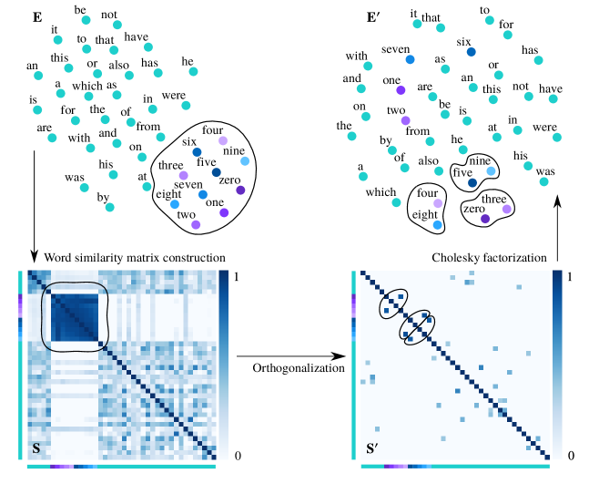
Figure 1: T-sne visualizations of non-regularized word embeddings $\mathbf{E}$ (top left) and orthogonalized word embeddings $\mathbf{E}^{\prime}$ (top right) for the 40 most common words on the first 100 MiB of the English Wikipedia, and images of the word similarity matrices $\mathbf{S}$ (bottom left) and $\mathbf{S}^{\prime}$ (bottom right). Word similarity matrix construction uses the parameters $o=1$ and $t=-1$, and orthogonalization uses the parameter values $\text{Sym}=\text{$\text{\char 51}$},\text{Dom}=\text{$\text{\char 51}$},$ and $\text{Idf}=\text{$\text{\char 51}$}$. Notice how the cluster of numerals from $\mathbf{E}$ is separated in $\mathbf{E}^{\prime}$ due to the parameter value $\text{Idf}=\text{$\text{\char 51}$}$, which makes common words more likely to be mutually orthogonal.

4.2 Orthogonalization

Novotný (2018) shows that producing a sparse word similarity matrix $\mathbf{S}^{\prime}$ that stores at most $C$ largest values from every column of $\mathbf{S}$ reduces the worst-case time complexity of the scm to $\mathcal{O}(p_{\mathbf{x}})$, where $p_{\mathbf{x}}$ is the number of unique words in a document vector $\mathbf{x}$.

Novotný also claims that $\mathbf{S}^{\prime}$ improves the performance of the soft vsm on the question answering task and describes a greedy algorithm for producing $\mathbf{S}^{\prime}$, which we will refer to as the orthogonalization algorithm. The orthogonalization algorithm has three boolean parameters: Sym, Dom, and Idf. Sym and Dom make $\mathbf{S}^{\prime}$ symmetric and strictly diagonally dominant. Idf processes columns of $\mathbf{S}$ in descending order of inverse document frequency (Robertson, 2004):

$$\text{inverse document frequency of word }w=-\log_{2}\text{P}(w\mid D)=\log_{2}\frac{|D|}{|\{d\in D\mid w\in d\}|}\text{, where }D\text{ are documents.}$$ (7)

In our experiment, we compute the scm directly from the word similarity matrix $\mathbf{S}^{\prime}$, see Equation (3). However, actual word embeddings must be extracted for many nlp tasks. Novotný shows that the word similarity matrix $\mathbf{S}^{\prime}$ can be decomposed using Cholesky factorization. We will now define orthogonalized word embeddings and we will show that the Cholesky factors of $\mathbf{S}^{\prime}$ are in fact orthogonalized word embeddings.

Definition 1 (Orthogonalized word embeddings)

Let $\mathbf{E},\mathbf{E}^{\prime}$ be real matrices with $|V|$ rows, where $V$ is a vocabulary of words. Then $\mathbf{E}^{\prime}$ are orthogonalized word embeddings from $\mathbf{E}$, which we denote $\mathbf{E}^{\prime}\leq_{\bot}\mathbf{E}$, iff for all $i,j=1,2,\ldots,|V|$ it holds that $\langle\mathbf{e}^{\prime}_{i},\mathbf{e}^{\prime}_{j}\rangle\neq 0\implies\langle\mathbf{e}^{\prime}_{i},\mathbf{e}^{\prime}_{j}\rangle=\langle\mathbf{e}_{i},\mathbf{e}_{j}\rangle$, where $\mathbf{e}_{k}$ and $\mathbf{e}^{\prime}_{k}$ denote the $k$-th rows of $\mathbf{E}$ and $\mathbf{E}^{\prime}$.

Theorem 4.1

Let $\mathbf{E}$ be a real matrix with $|V|$ rows, where $V$ is a vocabulary of words, and for all $k=1,2,\ldots,|V|$ it holds that $\|\mathbf{e}_{k}\|_{2}=1$. Let $\mathbf{S}$ be a word similarity matrix constructed from $\mathbf{E}$ with the parameter values $t=-1$ and $o=1$ as described in Section 3.2. Let $\mathbf{S}^{\prime}$ be a word similarity matrix produced from $\mathbf{S}$ using the orthogonalization algorithm with the parameter values $\text{Sym}=\text{$\text{\char 51}$}$ and $\text{Dom}=\text{$\text{\char 51}$}$. Let $\mathbf{E}^{\prime}$ be the Cholesky factor of $\mathbf{S}^{\prime}$. Then $\mathbf{E}^{\prime}\leq_{\bot}\mathbf{E}$.

Proof

With the parameter values $\text{Sym}=\text{$\text{\char 51}$},\text{Dom}=\text{$\text{\char 51}$}$, $\mathbf{S}^{\prime}$ is symmetric and strictly diagonally dominant, and therefore also positive definite. The symmetric positive definite matrix $\mathbf{S}^{\prime}$ has a unique Cholesky factorization of the form $\mathbf{S}^{\prime}=\mathbf{E}^{\prime}(\mathbf{E}^{\prime})^{\raisebox{-0.3014pt}{$\scriptscriptstyle\mkern-1.5mu\mathsf{T}$}}$. Therefore, the Cholesky factor $\mathbf{E}^{\prime}$ exists and is uniquely determined.

From $\mathbf{S}^{\prime}=\mathbf{E}^{\prime}(\mathbf{E}^{\prime})^{\raisebox{-0.3014pt}{$\scriptscriptstyle\mkern-1.5mu\mathsf{T}$}}$, we have that for all $i,j=1,2,\ldots,|V|$ such that the sparse matrix $\mathbf{S}^{\prime}$ does not contain the value $s^{\prime}_{ij}$ it holds that $s^{\prime}_{ij}=\langle\mathbf{e}^{\prime}_{i},\mathbf{e}^{\prime}_{j}\rangle=0$. Since the implication in the theorem only applies when $\langle\mathbf{e}^{\prime}_{i},\mathbf{e}^{\prime}_{j}\rangle\neq 0$, we do not need to consider this case.

From $\mathbf{S}^{\prime}=\mathbf{E}^{\prime}(\mathbf{E}^{\prime})^{\raisebox{-0.3014pt}{$\scriptscriptstyle\mkern-1.5mu\mathsf{T}$}},o=1,t=-1,$ and $\|\mathbf{e}_{k}\|_{2}=1$, we have that for all $i,j=1,2,\ldots,|V|$ such that the sparse matrix $\mathbf{S}^{\prime}$ contains the value $s^{\prime}_{ij}$, it holds that $\langle\mathbf{e}^{\prime}_{i},\mathbf{e}^{\prime}_{j}\rangle=s^{\prime}_{ij}=s_{ij}=\max(t,\langle\mathbf{e}_{i}/\|\mathbf{e}_{i}\|_{2},\mathbf{e}_{j}/\|\mathbf{e}_{j}\|_{2}\rangle)^{o}=\langle\mathbf{e}_{i},\mathbf{e}_{j}\rangle.$∎

Figure 1 shows the extraction of orthogonalized word embeddings $\mathbf{E}^{\prime}$ from $\mathbf{E}$: From $\mathbf{E}$, we construct the dense word similarity matrix $\mathbf{S}$ and from $\mathbf{S}$, we produce the sparse word similarity matrix $\mathbf{S}^{\prime}$ through orthogonalization. From $\mathbf{S}^{\prime}$, we produce the orthogonalized embeddings $\mathbf{E}^{\prime}$ through Cholesky factorization.

With a large vocabulary $V$, a $|V|\times|V|$ dense matrix $\mathbf{S}$ may not fit in the main memory, and we produce the sparse matrix $\mathbf{S}^{\prime}$ directly from $\mathbf{E}$. Similarly, a $|V|\times|V|$ dense matrix $\mathbf{E}^{\prime}$ may also not fit in the main memory, and we use sparse Cholesky factorization to produce a sparse matrix $\mathbf{E}^{\prime}$ instead. If dense word embeddings are required, we use dimensionality reduction on $\mathbf{E}^{\prime}$ to produce a $|V|\times D$ dense matrix, where $D$ is the number of dimensions.

With the parameter value $\text{Idf}=\text{$\text{\char 51}$},$ words with small inverse document frequency, i.e. common words such as numerals, prepositions, and articles, are more likely to be mutually orthogonal (i.e. $\langle\mathbf{e}^{\prime}_{i},\mathbf{e}^{\prime}_{j}\rangle=0$) than rare words. This is why in Figure 1, the numerals form a cluster in the non-regularized word embeddings $\mathbf{E}$, but they are separated in orthogonalized word embeddings $\mathbf{E}^{\prime}$.

5 Experiment

The experiment was conducted using six standard text classification datasets by employing both the wmd and the scm with a $k$ Nearest Neighbor ($k$nn) classifier using both regularized and non-regularized word embeddings. First, we describe briefly our datasets, then our experimental steps. Our experimental code is available online.

5.1 Datasets

In our experiment, we used the following six standard text classification datasets:

BBCSPORT

The bbcsport dataset (Greene and Cunningham, 2006) consists of 737 sport news articles from the bbc sport website in five topical areas: athletics, cricket, football, rugby, and tennis. The period of coverage was during 2004–2005.

TWITTER

The twitter dataset (Sanders, 2011) consists of 5,513 tweets hand-classified into one of four topics: Apple, Google, Twitter, and Microsoft. The sentiment of every tweet was also hand-classified as either Positive, Neutral, Negative, or Irrelevant.

OHSUMED

The ohsumed dataset (Hersh et al., 1994) is a set of 348,566 references spanning 1987–1991 from the medline bibliographic database of important, peer-reviewed medical literature maintained by the National Library of Medicine (nlm). While the majority of references are to journal articles, there are also a small number of references to letters of the editor, conference proceedings, and other reports. Each reference contains human-assigned subject headings from the 17,000-term Medical Subject Headings (MeSH) vocabulary.

REUTERS

The documents in the reuters-21578 collection (Lewis, 1997) appeared on the Reuters newswire in 1987. The documents were assembled and indexed with categories by the personnel of Reuters Ltd. The collection is contained in 22 sgml files. Each of the first 21 files (reut2-000.sgm through reut2-020.sgm) contains 1,000 documents, while the last one (reut2-021.sgm) contains only 578 documents.

AMAZON

The amazon dataset (McAuley et al., 2015) contains 142.8 million product reviews from Amazon spanning 1996–2014. Each product belongs to one of 24 categories, which include Books, Cell Phones & Accessories, Clothing, Shoes & Jewelry, Digital Music, and Electronics, among others. The $5$-core subset of the amazon dataset contains only those products and users with at least five reviews.

20NEWS

The 20news dataset (Lang, 1995) is a collection of 18,828 Usenet newsgroup messages partitioned across 20 newsgroups with different topics. The collection has become popular for experiments in text classification and text clustering.

5.2 Preprocessing

For twitter, we use 5,116 out of 5,513 tweets due to unavailability, we restrict our experiment to the Positive, Neutral, and Negative classes, and we subsample the dataset to 3,108 tweets like Kusner et al. (2015). For ohsumed, we use the 34,389 abstracts related to cardiovascular diseases (Joachims, 1998) out of 50,216 and we restrict our experiment to abstracts with a single class label from the first 10 classes out of 23. In the case of reuters, we use the R8 subset (Cardoso-Cachopo, 2007). For amazon, we use 5-core reviews from the Books, CDs and Vinyl, Electronics, and Home and Kitchen classes.

We preprocess the datasets by lower-casing the text and by tokenizing to longest non-empty sequences of alphanumeric characters that contain at least one alphabetical character. We do not remove stop words or rare words, only words without embeddings. We split each dataset into train and test subsets using either a standard split (for reuters and 20news) or following the split size of Kusner et al. (2015). See Table 1 for statistics of the preprocessed datasets.

Algorithm 1  The $k$nn classifier for the wmd and the scm with regularized and non-regularized word embeddings

Input: Training data $A$, test data $B$, neighborhood size $k$
      Output: Class labels for the test data, $L$

1:foreach $b_{i}\in B$ do

2:     For all $a_{j}\in A$, compute the scm / wmd between $a_{j}$ and $b_{i}$.

3:     Choose the $k$ nearest neighbors of $b_{i}$ in $A$.

4:     Assign the majority class of the $k$ nearest neighbors to $l_{i}$.

5:end for

Table 1: Statistics of the datasets used for evaluation, where $E[p]$ is the average number of unique words in a document, and $|\mathcal{Y}|$ is the number of document classes

Dataset name	Train set size	Test set size	$E[p]$	$|\mathcal{Y}|$
bbcsport	517	220	181.0	5
twitter	2,176	932	13.7	3
ohsumed	3,999	5,153	89.4	10
reuters	5,485	2,189	56.0	8
amazon	5,600	2,400	86.3	4
20news	11,293	7,528	145.0	20

   
   

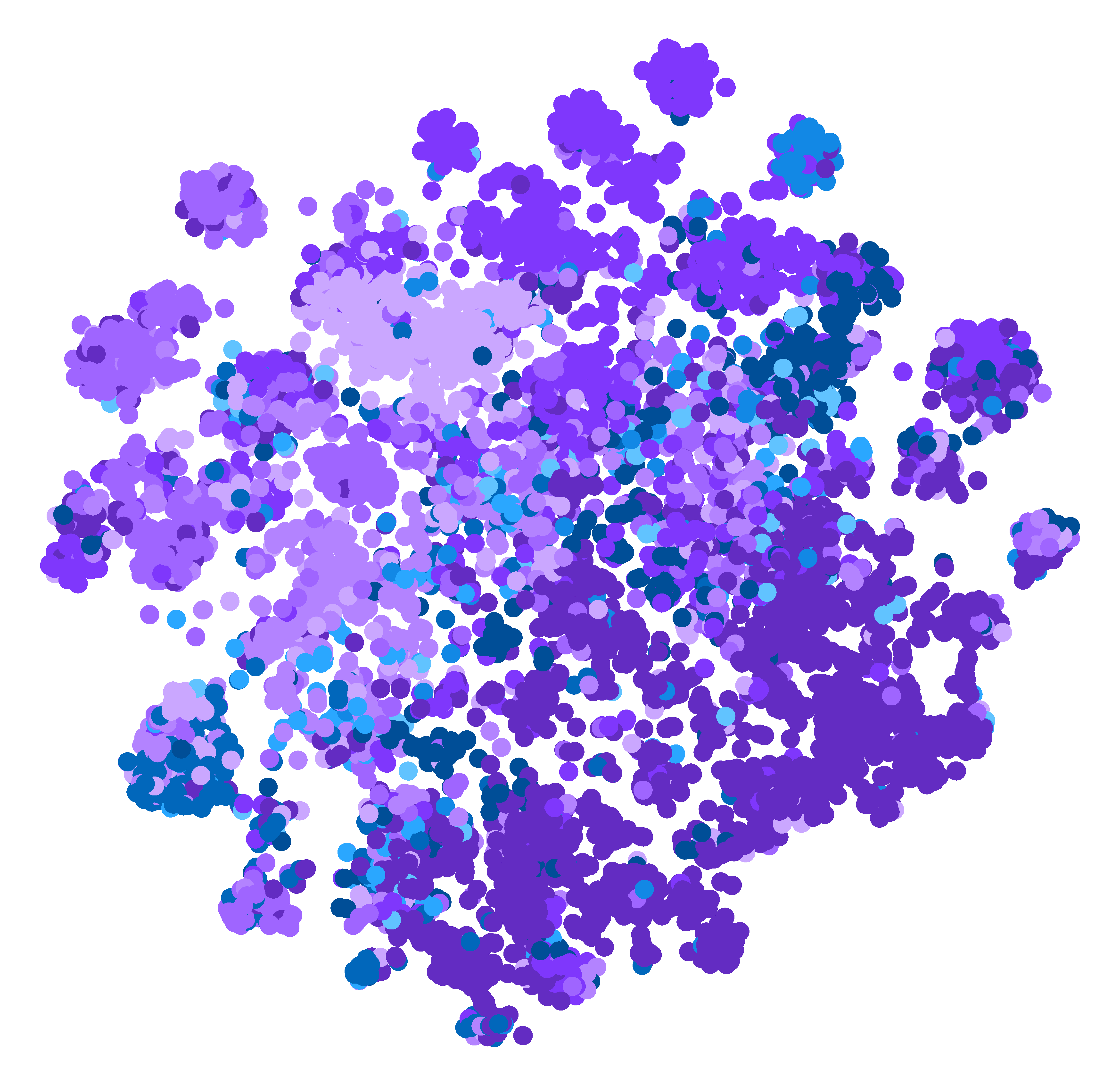
Figure 2: $k$nn ($k=9$) confusion matrices and t-sne document visualizations for the soft vsm with non-regularized (50.71% test error, top) and regularized (24.14% test error, bottom) word embeddings on the ohsumed dataset. See https://mir.fi.muni.cz/ohsumed-nonregularized and https://mir.fi.muni.cz/ohsumed-regularized for interactive three-dimensional t-sne document visualisations.

       
   

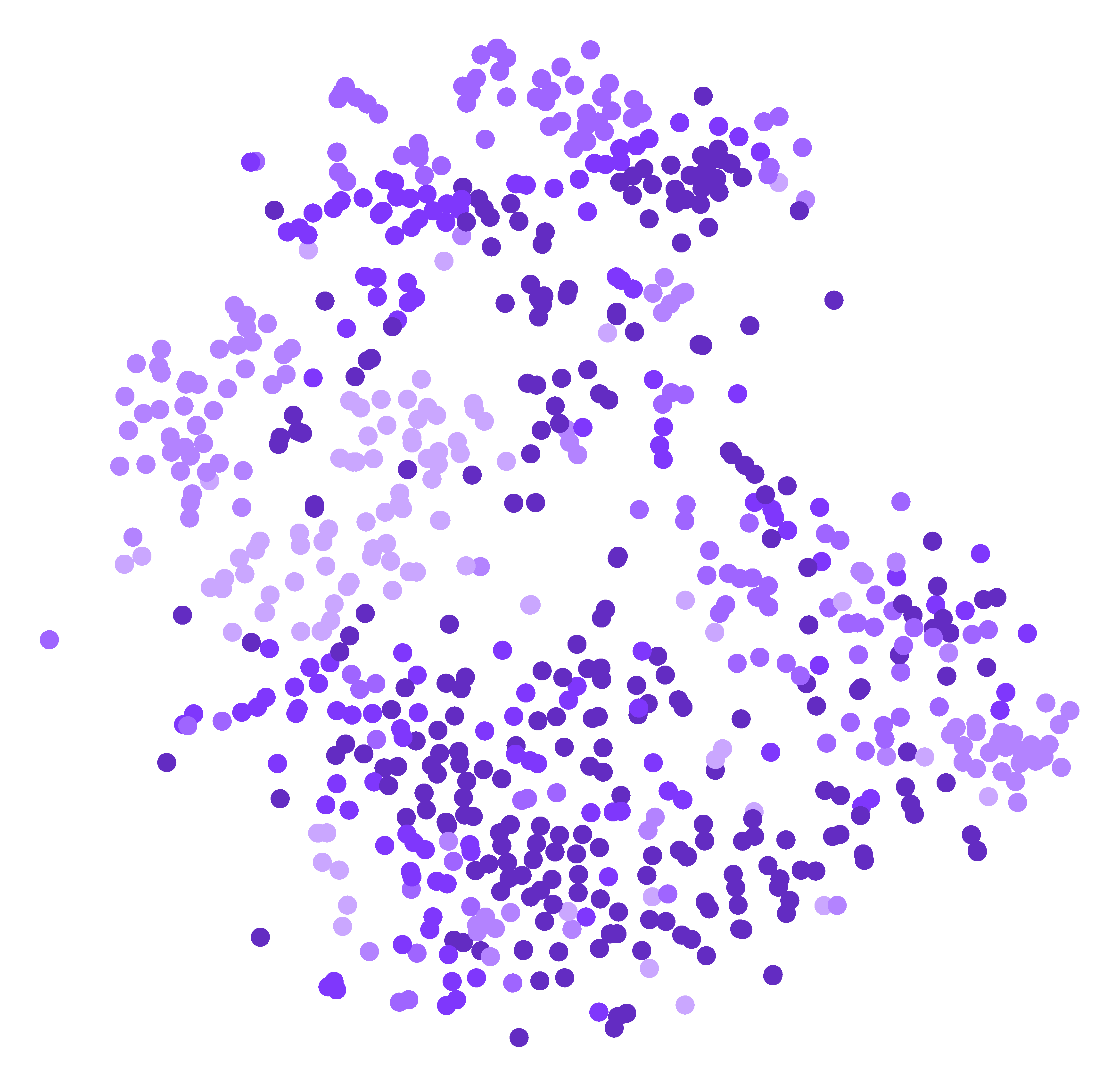
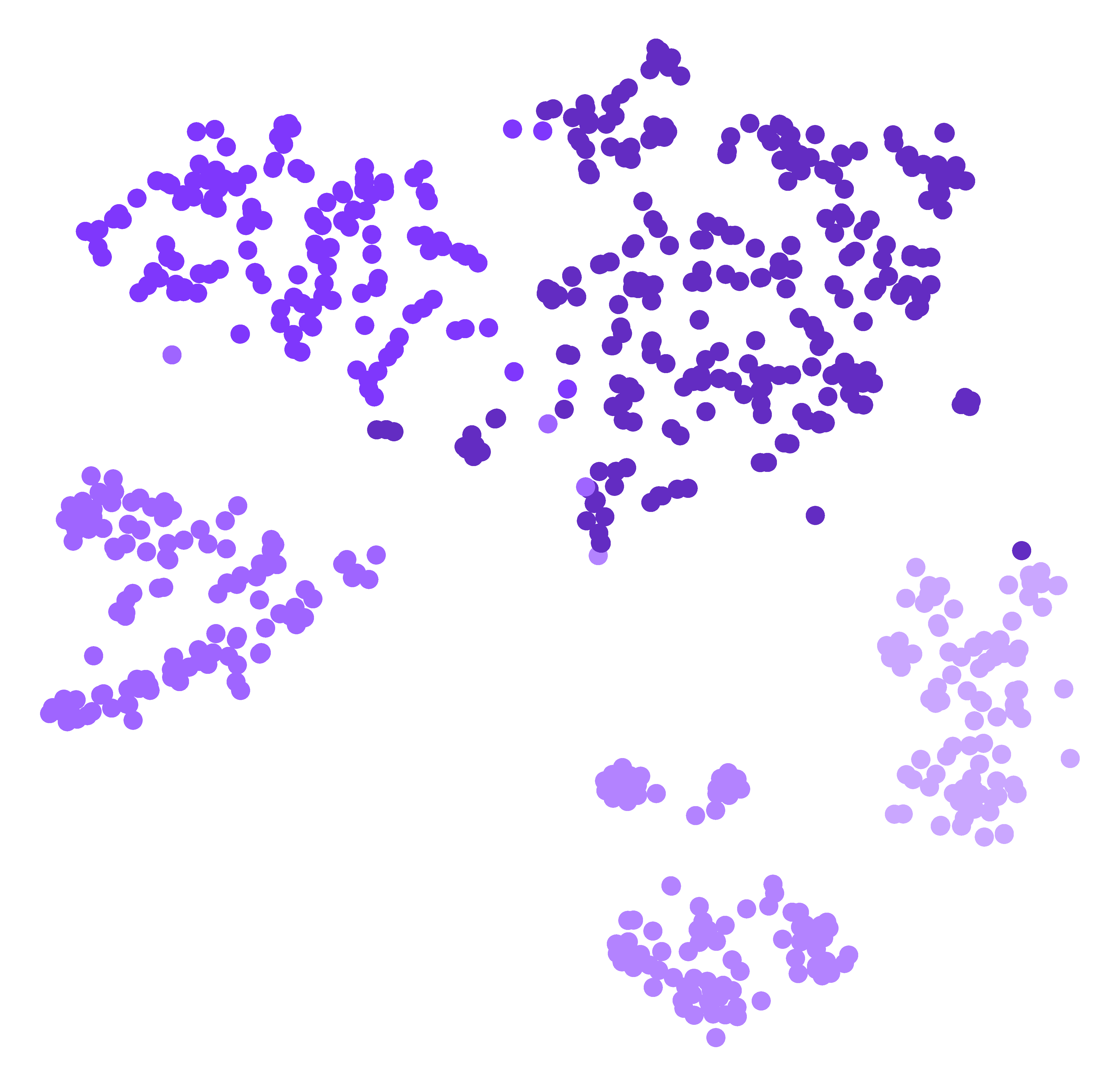
Figure 3: $k$nn ($k=1$) confusion matrices and t-sne document visualizations for the soft vsm with non-regularized (21.82% test error, top) and regularized (2.27% test error, bottom) word embeddings on the bbcsport dataset. See https://mir.fi.muni.cz/bbcsport-nonregularized and https://mir.fi.muni.cz/bbcsport-regularized for interactive three-dimensional t-sne document visualisations.

   
   

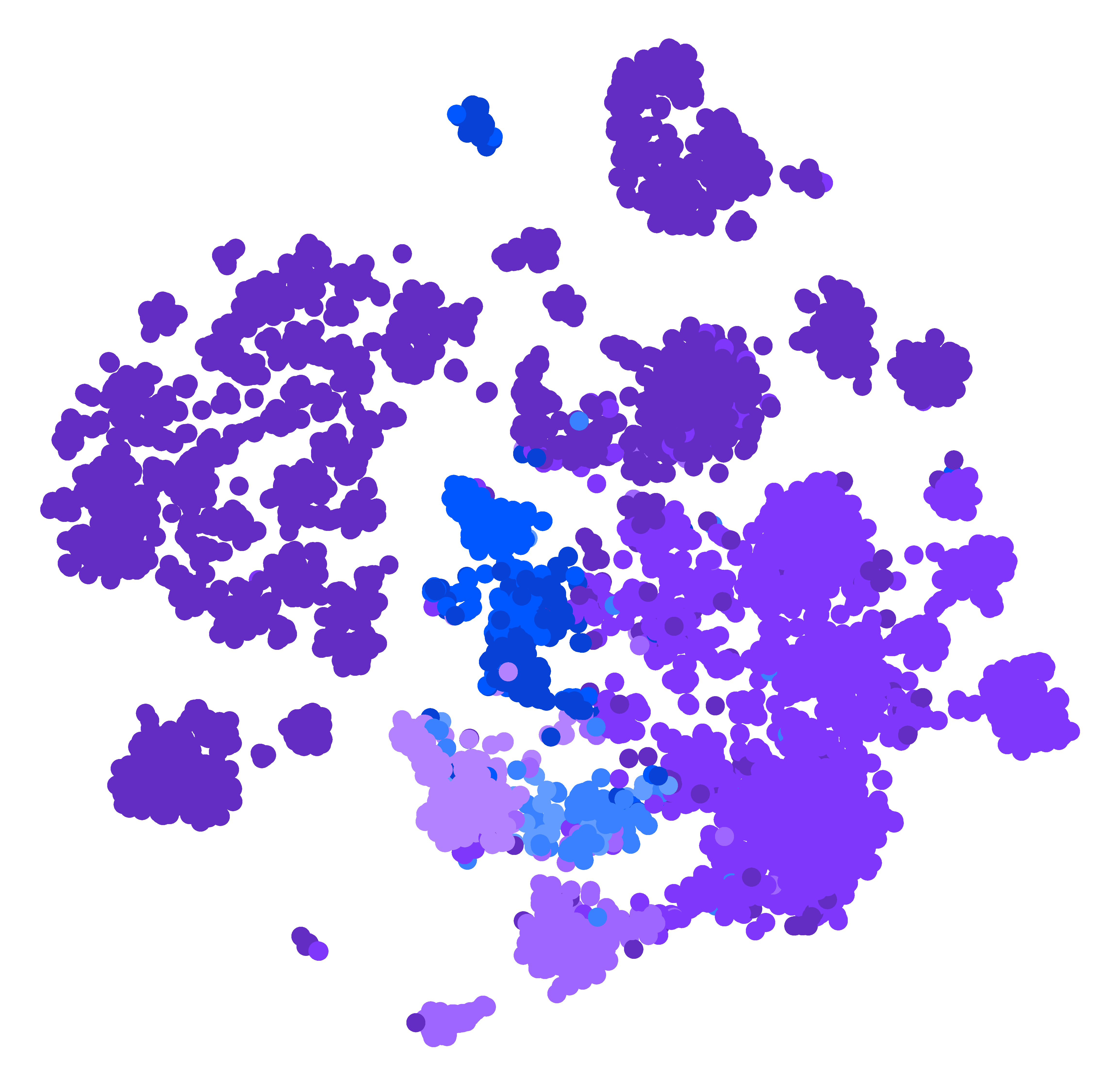
Figure 4: $k$nn ($k=9$ and $19$) confusion matrices and t-sne document visualizations for the soft vsm with non-regularized (10.19% test error, top) and regularized (7.22% test error, bottom) word embeddings on the reuters dataset. See https://mir.fi.muni.cz/reuters-nonregularized and https://mir.fi.muni.cz/reuters-regularized for interactive three-dimensional t-sne document visualisations.

          
   

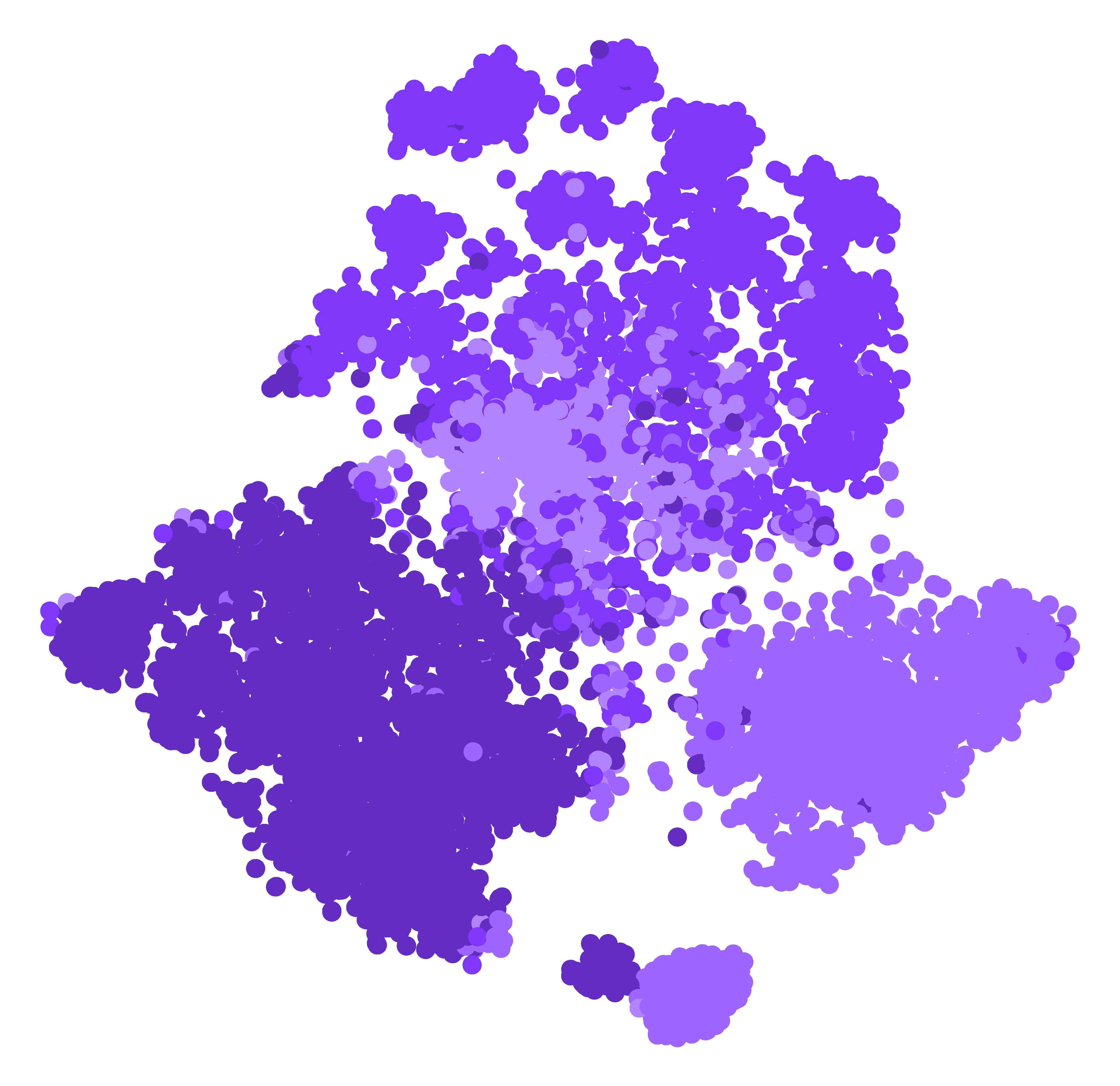
Figure 5: $k$nn ($k=15$ and $11$) confusion matrices and t-sne document visualizations for the soft vsm with non-regularized (10.04% test error, top) and regularized (6.33% test error, bottom) word embeddings on the amazon dataset. See https://mir.fi.muni.cz/amazon-nonregularized and https://mir.fi.muni.cz/amazon-regularized for interactive three-dimensional t-sne document visualisations.

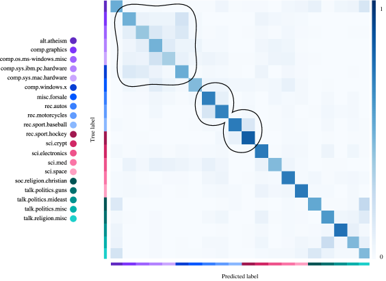
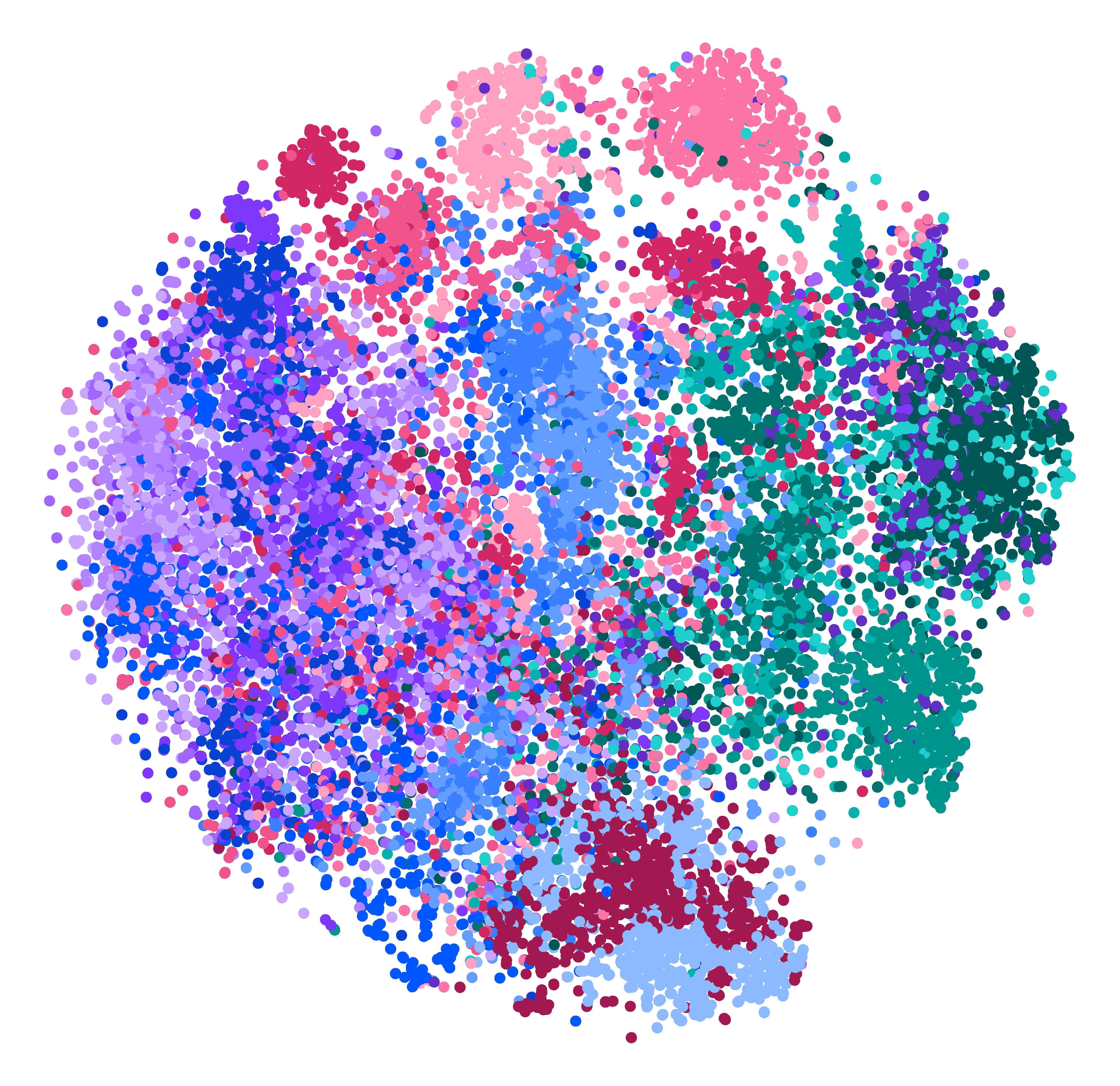
Figure 6: $k$nn ($k=1$) confusion matrix (top) and t-sne document visualization (bottom) for the soft vsm with non-regularized (42.53% test error) word embeddings on the 20news dataset. Notice how the Usenet hierarchies comp.*, rec.*, and rec.sport.* form visible clusters. See https://mir.fi.muni.cz/20news-nonregularized for an interactive three-dimensional t-sne document visualisation.

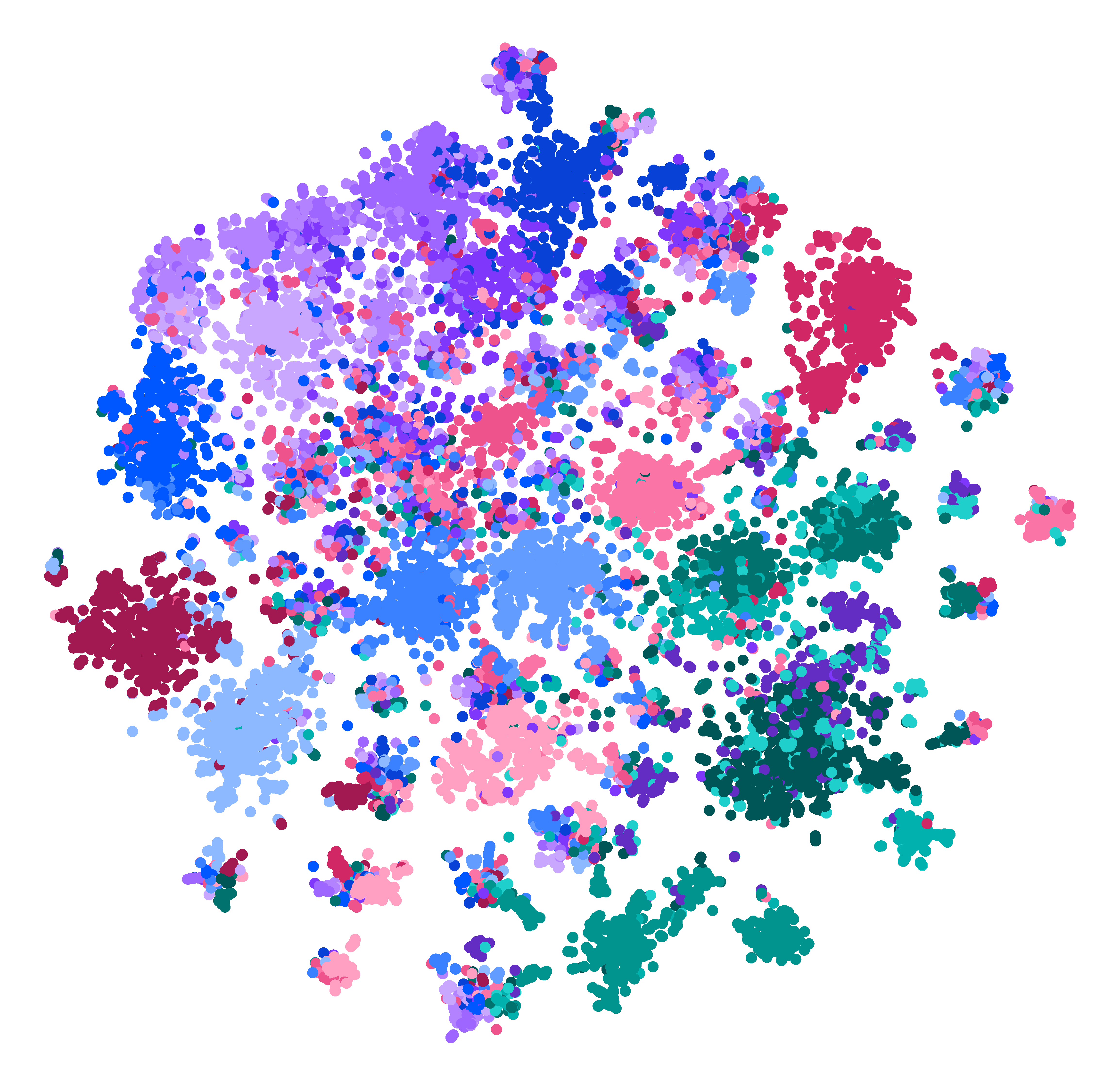
Figure 7: $k$nn ($k=1$) confusion matrix (top) and t-sne document visualization (bottom) for the soft vsm with regularized (29.97% test error) word embeddings on the 20news dataset. See https://mir.fi.muni.cz/20news-regularized for an interactive three-dimensional t-sne document visualisation.

5.3 Training and Regularization of Word Embeddings

Using Word2Vec, we train the cbow on the first 100 MiB of the English Wikipedia (Mahoney, 2011) using the same parameters as Lam (2018, Section 4.3) and 10 training epochs. We use quantized word embeddings in 1,000 dimensions and non-quantized word embeddings in 200 dimensions to achieve comparable performance on the word analogy task. (Lam, 2018)

5.4 Nearest Neighbor Classification

We use the vsm with uniform word frequency weighting, also known as the bag of words (bow), as our baseline. For the scm, we use the double-logarithm inverse collection frequency word weighting (the smart dtb weighting scheme) as suggested by Singhal et al. (2001, Table 1). For the wmd, we use bow document document vectors like Kusner et al. (2015).

We tune the parameters $o\in\{1,2,3,4\}$ and $t\in\{0,\pm\nicefrac{{1}}{{2}},1\}$ of the scm, the parameter $s\in\{0.0,0.1,\ldots,1.0\}$ of the smart dtb weighting scheme, the parameter $k\in\{1,3,\ldots,19\}$ of the $k$nn, and the parameters $C\in\{100,200,400,800\}$, and Idf, Sym, Dom${}\in\{\text{\char 51},\text{\char 55}\}$ of the orthogonalization. For each dataset, we hold out 20% of the train set for validation, and we use grid search to find the optimal parameter values. To classify each sample in the test set, we follow the procedure presented in Algorithm 1.

5.5 Significance Testing

We use the method of Agresti and Coull (1998) to construct 95% confidence intervals for the $k$nn test error. For every dataset, we use Student’s $t$-test at 95% confidence level with $q$-values (Benjamini and Hochberg, 1995) for all combinations of document similarities and word embedding regularization techniques to find significant differences in $k$nn test error.

6 Discussion of Results

Our results are shown in figures 2–11 and in Table 2. In the following subsections, we will discuss the individual results and how they are related.

6.1 Task Performance on Individual Datasets

Figure 8 shows 95% interval estimates for the $k$nn test error. All differences are significant, except for the second and fourth results from the left on the bbcsport and twitter datasets, the sixth and seventh results from the left on the bbcsport and ohsumed datasets, and the fourth and sixth results from the left on the twitter dataset.

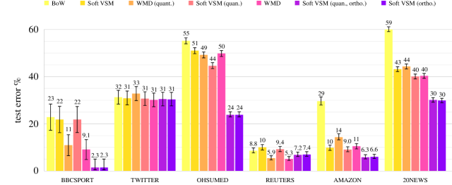
Figure 8: 95% interval estimates for the $k$nn test error on six text classification datasets

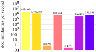
Figure 9: Average document processing speed on one Intel Xeon X7560 core

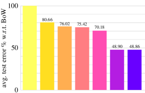
Figure 10: Average $k$nn test error compared to the bow

Although most differences in the $k$nn test error are statistically significant on the twitter dataset, they are relatively minor compared to other datasets. This is because of two reasons: (1) twitter is a sentiment analysis dataset, and (2) words with opposite sentiment often appear in similar sentences. Since word embeddings are similar for words that appear in similar sentences, embeddings for words with opposite sentiment are often similar. For example, the embeddings for the words good and bad are mutual nearest neighbors with cosine similarity 0.58 for non-quantized and 0.4 for quantized word embeddings. As a result, word embeddings don’t help us separate positive and negative documents. Using a better measure of sentiment in the word similarity matrix $\mathbf{S}$ and in the flow cost $c_{ij}$ would improve the task performance of the soft vsm and the wmd.

Figures 2–7 show confusion matrices and t-sne document visualizations (Maaten and Hinton, 2008) for the soft vsm with non-regularized word embeddings and for the soft vsm with orthogonalized and quantized word embeddings.

In Figure 2, we see that with non-regularized word embeddings, we predict most documents as class C04, followed by classes C10 and C06. When a document representation is uniformly random, then the most common classes in a dataset are most likely to be predicted by the $k$nn classifier. In the ohsumed dataset, 2,835 documents belong to the most common class C04, 1,711 documents belong to the second most common class C10, and 1,246 documents belong to the third most common class C06. In contrast to the almost random representations of the soft vsm with non-regularized word embeddings, orthogonalized word embeddings make the true class label much easier to predict. We hypothesize that this is because ohsumed is a medical dataset. Medical terms are highly specific, so when we search for documents containing similar words, we need to restrict ourselves only to highly similar words, which is one of the effects of using orthogonalized word embeddings.

In Figure 4, we see that with non-regularized word embeddings, most documents from the class Grain are misclassified as the more common class Crude. With regularized word embeddings, the classes are separated. We hypothesize that this is because both grain and crude oil are commodities, which makes the documents from both classes contain many similar words. The classes will become indistinguishable unless we restrict ourselves only to a subset of the similar words, which is one of the effects of using orthogonalized word embeddings.

In Figure 6, we see that with non-regularized word embeddings, messages are often misclassified as a different newsgroup in the same Usenet hierarchy. We can see that the Usenet hierarchies comp.*, rec.*, and rec.sport.* form visible clusters in both the t-sne document visualization and in the confusion matrix. In Figure 7, we see that with regularized word embeddings, the clusters are separated. We hypothesize that this is because newsgroups in a Usenet hierarchy share a common topic and similar terminology. The terminology of the newsgroups will become difficult to separate unless only highly specific words are allowed to be considered similar, which is one of the effects of using orthogonalized word embeddings.

6.2 Average Task Performance

Figure 10 shows the average $k$nn test error ratio between the document similarities and the bow baseline. This ratio is the lowest for the soft vsm with orthogonalized word embeddings, which achieves $48.86\%$ of the average bow $k$nn test error. The average test error ratio between the soft vsm with regularized word embeddings and the soft vsm with non-regularized word embeddings is $60.57\%$, which is a $39.43\%$ reduction in the average $k$nn test error.

Unlike the soft vsm, the wmd does not benefit from word embedding quantization. This is because of two reasons: (1) the soft vsm takes into account the similarity between all words in two documents, whereas the wmd only considers the most similar word pairs, and (2) non-quantized word embeddings are biased towards positive similarity, see Figure 11. With non-quantized word embeddings, embeddings of unrelated words have positive cosine similarity, which makes dissimilar documents less separable. With quantized embeddings, unrelated words have negative cosine similarity, which improves separability and reduces $k$nn test error. The wmd is unaffected by the bias in non-quantized word embeddings, and the reduced precision of quantized word embeddings increases $k$nn test error.

6.3 Document Processing Speed

Figure 9 shows the average document processing speed using a single Intel Xeon X7560 2.26 GHz core. Although the orthogonalization reduces the worst-case time complexity of the soft vsm from quadratic to linear, it also makes the word similarity matrix sparse, and performing sparse instead of dense matrix operations causes a $2.73\times$ slowdown compared to the soft vsm with non-orthogonalized word embeddings. Quantization causes a $1.8\times$ slowdown, which is due to the $5\times$ increase in the word embedding dimensionality, since we use 1000-dimensional quantized word embeddings and only 200-dimensional non-quantized word embeddings.

The super-cubic average time complexity of the wmd results in an average $819{,}496\times$ slowdown compared to the soft vsm with orthogonalized and quantized word embeddings, and a $1{,}505{,}386\times$ slowdown on the 20news dataset, which has a large average number of unique words in a document. Although Kusner et al. (2015) report up to $110\times$ speed-up using an approximate variant of the wmd (the wcd), this still results in an average $7{,}450\times$ slowdown, and a $13{,}685\times$ slowdown on the 20news dataset.

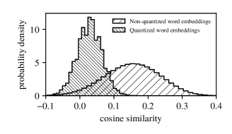
Figure 11: Histograms of word embedding cosine similarity

Table 2: Optimal parameter values for the soft vsm with orthogonalized word embeddings. Most common parameter values are bold.

Dataset name	$o$	$s$	$t$	$C$	$k$	Idf	Sym	Dom
bbcsport	2	0	$\mathbf{-1}$	100	1	✔	✔	✔
twitter	2	0	$\mathbf{-1}$	400	13	✔	✔	✗
ohsumed	4	0	$\mathbf{-1}$	200	11	✔	✗	✔
reuters	4	0	$\mathbf{-1}$	100	19	✔	✔	✔
amazon	4	0	$\mathbf{-1}$	100	17	✔	✔	✔
20news	3	0	$\mathbf{-1}$	100	1	✔	✗	✗

6.4 Parameter Optimization

Table 2 shows the optimal parameter values for the soft vsm with orthogonalized word embeddings. The most common parameter value $\text{Idf}=\text{\char 51}$ shows that it is important to store the nearest neighbors of rare words in the word similarity matrix $\mathbf{S}^{\prime}$. The most common parameter values $C=100$, $o=4$, $t=-1$, $\text{Sym}=\text{\char 51}$, and $\text{Dom}=\text{\char 51}$ show that strong orthogonalization, which makes most values in $\mathbf{S}^{\prime}$ zero or close to zero, gives the best results.

Due to the low document processing speed of the wmd and the number of orthogonalization parameters, using parameter optimization on the wmd with regularized embeddings is computationally intractable. Therefore, we do not report results for the wmd with regularized embeddings in figures 8–10.

7 Conclusion

Word embeddings achieve state-of-the-art results on several nlp tasks, predominantly at the sentence level, but overfitting is a major issue, especially when applied at the document level with a large number of words. We have shown that regularization of word embeddings significantly improves their performance not only on the word analogy, word similarity, and semantic text similarity tasks, but also on the text classification task.

We further show that the most effective word embedding regularization technique is orthogonalization and we prove a connection between orthogonalization, Cholesky factorization and orthogonalized word embeddings. With word embedding orthogonalization, the task performance of the soft vsm exceeds the wmd, an earlier known state-of-the-art document distance measure, while being several orders of magnitude faster. This is an important step in bringing application of word embeddings from supercomputers to mobile and embedded systems.