Decoherence as Detector of the Unruh Effect

Abstract

We propose a new type of the Unruh-DeWitt detector which measures the decoherence of the reduced density matrix of the detector interacting with the massless quantum scalar field. We find that the decoherence decay rates are different in the inertial and accelerated reference frames. We show that the exponential phase decay can be observed for relatively low accelerations, that can significantly improve the conditions for measuring the Unruh effect.

All elementary particles, which exist in nature, are the excitations of the corresponding quantum fields. But even when these fields are in their quantum vacuum states, a very complicated dynamics of vacuum fluctuations takes place. Moreover, as it was discovered by Unruh in 1976 Unruh (1976), in a flat spacetime the state of the quantum vacuum depends on the motion of observer, and thus the concept of particles, in the context of quantum field theory, is relative. More specifically, for the uniformly accelerated observer the vacuum of quantum fields in the Minkowski spacetime is modified to the thermal state. This result, nowadays known as the Unruh effect, generated an enormous number of publications. (See Ref. L. C. B. Crispino, A. Higuchi and G. E. A. Matsas (2008) for a comprehensive review, and references therein.) The effective temperature of the thermal distribution is $T=\hbar a/2\pi ck_{B}$, where $a$ is the acceleration, $k_{B}$ is the Boltzmann constant, $\hbar$ is the reduced Planck constant, and $c$ is the speed of light.

The direct observation of the Unruh effect requires very large accelerations, e. g. $a\approx 2.5\cdot 10^{20}\,\rm m/s^{2}$ for $T=1K$. These accelerations can be realized only in strong gravitational fields, for instance, produced by the black holes. That is why, the current trend in this field is to propose various types of detectors which can measure indirectly the Unruh effect W. G. Unruh (1995); W. G. Unruh and R. M. Wald (1984); D. Hümmer, E. Martín-Martínez and A. Kempf (2016); W. Zhou, R. Passante and L. Rizzuto (2016); F. Hong-Yi (2010). In particular, the detector which measures the dependence of the Berry phase on the acceleration was suggested in E. Martín-Martínez, I. Fuentes and R. B. Mann (2011); E. Martín-Martínez, A. Dragan, R. B. Mann and I. Fuentes (2013). According to Ref. E. Martín-Martínez, I. Fuentes and R. B. Mann (2011), this detector can significantly reduce the required acceleration, up to $a\approx 2.5\cdot 10^{17}\,\rm m/s^{2}$.

In this Letter, we propose a new type of detector to probe the Unruh effect. Our detector does not measure directly the equilibrium distribution of the produced particles, but the decoherence of the reduced density matrix. We show that this information can be used for the detection of the Unruh effect at significantly lower accelerations, even in comparison with the detector based on the measurement of the Berry phase. Through the paper, unless stated otherwise, we use the natural units, $\hbar=c=k_{B}=1$.

We assume that the observer moves with an uniform acceleration, $a$, in $z$-direction with respect to an inertial reference frame in the Minkowski spacetime. The transformation of coordinates,

$$t=\frac{1}{a}e^{a\zeta}\sinh(a\tau),\quad z=\frac{1}{a}e^{a\zeta}\cosh(a\tau),$$ (1)

describes the right wedge of the Rindler spacetime with the metric,

$$ds^{2}=e^{2a\zeta}(d\tau^{2}-d\zeta^{2})-d\textbf{x}_{\bot}^{2},$$ (2)

where we set ${\mathbf{x}}_{\perp}=(x,y)$. Hereafter, we denote the coordinates in the Minkowski spacetime as $(t,\mathbf{r})$, and the coordinates in the Rindler spacetime as $(\tau,\mathbf{x})$, where $\mathbf{x}=({\mathbf{x}}_{\perp},\zeta)$.

The conventional Unruh-DeWitt (UDW) detector is presented as a box containing a non-relativistic particle interacting with a massless scalar field. It is assumed that the detector is located at the origin of the moving reference frame, and the particle is in its ground state. The quanta of the scalar field is detected if the detector is found in an excited state. Since, only two states are relevant: the ground state and the first excited state, one can consider the detector as a two-level quantum system interacting with the scalar field Unruh (1976); W. G. Unruh and R. M. Wald (1984).

The entire system, “detector + field”, is governed by the Hamiltonian, $\mathcal{H}_{t}=H_{d}+H_{f}+H_{int}$, where $H_{d}$ is the Hamiltonian of the detector, $H_{f}$ is the Hamiltonian of the free scalar field, and $H_{int}$ stands for the interaction Hamiltonian. The latter can be written as, $H_{int}=\int_{\Sigma_{t}}{\mathcal{H}}_{int}\,d^{3}\mathbf{r}$, where ${\mathcal{H}}_{int}$ is the Hamiltonian density, and the integral is taken over the three-dimensional surface, $\Sigma_{t}$, at time $t=\rm const$.

In the original formulation, of the UDW model, the detector was considered as a pointlike particle, with the interaction Hamiltonian being $H_{int}=\int_{\Sigma_{t}}\delta^{3}(\mathbf{r}-\mathbf{r}(t)){\mathcal{H}}_{int}\,d^{3}\mathbf{r}$, where $\mathbf{r}(t)$, describes the trajectory of the detector. In our paper we consider both cases: a pointlike detector and a detector of the finite size.

In our analysis, we consider the UDW detector as a two-level system with the transition energy $\varepsilon$. The Hamiltonian of the detector we take as $H_{d}=(\varepsilon/2)\sigma_{z}$, where $\sigma_{z}$ is the Pauli matrix. This form of the Hamiltonian corresponds to the effective Zeeman interaction of a single spin with a permanent magnetic field, oriented in the $z$-direction.

We assume that in the uniformly accelerated reference frame, the detector is located at the origin of the coordinates. The entire system is governed by the Hamiltonian,

$$H_{t}={{\varepsilon}\over{2}}\sigma_{z}\otimes\mbox{$1{\bf l}$}+\mbox{$1{\bf l}$}\otimes\sum_{\omega>0}\sum_{\textbf{k}_{\bot}}\omega b^{\dagger}_{\mathbf{k}}b_{\mathbf{k}}$$

$$+\frac{\lambda}{\sqrt{V}}\sigma_{z}\otimes\sum_{\omega>0}\sum_{\textbf{k}_{\bot}}\frac{1}{\sqrt{2\omega}}(g_{\mathbf{k}}b^{\dagger}_{\mathbf{k}}+g^{\ast}_{\mathbf{k}}b_{\mathbf{k}}),$$ (3)

where $\sigma_{z}$ is the Pauli matrix, $\lambda$ is a coupling constant and $\mathbf{k}=(\textbf{k}_{\bot},\omega)$. The Rindler creation and annihilation operators, associated with the field mode, $\mathbf{k}$, obey the standard commutation relations: $[b_{\mathbf{k}},b^{\dagger}_{{\mathbf{k}}^{\prime}}]=\delta_{{\mathbf{k}}{\mathbf{k}}^{\prime}}$, $[b_{\mathbf{k}},b_{{\mathbf{k}}^{\prime}}]=0$ and $[b^{\dagger}_{\mathbf{k}},b^{\dagger}_{{\mathbf{k}}^{\prime}}]=0$. The form factor, $g_{\mathbf{k}}$, is defined as follows: $g_{\mathbf{k}}=\int_{\mathbf{R}^{3}}v_{\mathbf{k}}({\mathbf{x}})f(\mathbf{x})e^{a\zeta}d\zeta\,d^{2}\mathbf{x}_{\perp}$. The modes, $v_{\mathbf{k}}$, are given by Fulling (1973, 1989); F. Lenz, K. Ohta and K. Yazaki (2008),

$$v_{\mathbf{k}}=\sqrt{\frac{4\omega\sinh(\pi\omega/a)}{\pi a}}K_{i\omega/a}\Big{(}\frac{k_{\bot}}{a}e^{a\zeta}\Big{)}e^{i\mathbf{k}_{\perp}\cdot\mathbf{x}_{\perp}},$$ (4)

where $K_{i\mu}(z)$ is the Macdonald function of the imaginary order. The function, $f(\mathbf{x})$, describes the spatial profile of the detector in the Rindler space.

In (3), we assume that the interaction term is much smaller than the effective Zeeman interaction. It is well-known that in this case, only the $\sigma_{z}$ operator can be used in the interaction Hamiltonian. We call the system with the Hamiltonian (3) energy conserving, because the operator, $\sigma_{z}$, commutes with the total Hamiltonian. As a result, the initial probabilities of population of the detector do not change in time.

We assume that for the entire system, the density operator, $\varrho(\tau)$, at time $\tau=\tau_{0}$, takes the form, $\varrho(\tau_{0})=|\Psi_{0}\rangle\langle\Psi_{0}|$, with $|\Psi_{0}\rangle=|\psi_{0}\rangle\otimes|0_{M}\rangle$. Here, $|\psi_{0}\rangle=\alpha|\downarrow\rangle+\beta|\uparrow\rangle$, denotes the initial superpositional state of the detector, and $|0_{M}\rangle$ stands for the Minkowski vacuum.

We denote by $\rho(\tau)$ the detector reduced density matrix, obtained by tracing out all scalar field degrees of freedom. The time evolution of the matrix elements of the reduced density matrix can be written as,

$$\rho_{ij}(\tau)= \langle i|{\rm Tr}_{R}U(\tau)\varrho(0)U^{-1}(\tau)|j\rangle,$$ (5)

$$(i,j=0,1),$$

where the index $i=0$ is associated with the eigenvector $|\downarrow\rangle$, and the index $i=1$ is associated with the eigenvector $|\uparrow\rangle$ of the operator $\sigma_{z}$.

The interaction of the detector with the scalar field does not excite the detector, and the detection of the Unruh effect is reduced to the study of the phase decoherence (decay of the non-diagonal elements of the reduced density matrix) (for details see the supplemental material (SM) at https:// …):

$$\rho_{01}(\tau)=e^{i\varepsilon\tau-\gamma(\tau)}\rho_{01}(\tau_{0}).$$ (6)

We say that the full phase decoherence takes place if $\rho_{01}(\tau)\rightarrow 0$ as $\tau\rightarrow\infty$. Otherwise, we call the phase decoherence partial.

The computation of the decoherence function yields (see SM):

$$\gamma(\tau)=\frac{\lambda^{2}}{2\pi^{3}}\int_{0}^{\infty}\frac{|g_{\omega}|^{2}}{\omega}{\rm sinc}^{2}\Big{(}\frac{\omega\tau}{2}\Big{)}\coth\Big{(}\frac{\pi\omega}{a}\Big{)}d\omega,$$ (7)

where $|g_{\omega}|^{2}=\int|g_{\mathbf{k}}|^{2}d^{2}{\mathbf{k}}_{\perp}$, ${\rm sinc}(x)=\sin(x)/x$.

Pointlike detector. – For a pointlike detector, the form factor is,

$$g_{\mathbf{k}}=\sqrt{\frac{4\omega\sinh(\pi\omega/a)}{\pi a}}K_{i\omega/a}\Big{(}\frac{k_{\bot}}{a}\Big{)}.$$ (8)

The computation of $|g_{\omega}|^{2}$ yields, $|g_{\omega}|^{2}=8\pi\omega^{2}$. Substituting this result in Eq. (7), we obtain,

$$\gamma(\tau)=\frac{4\lambda^{2}}{\pi^{2}}\int_{0}^{\infty}{\omega}\,{\rm sinc}^{2}\Big{(}\frac{\omega\tau}{2}\Big{)}\coth\Big{(}\frac{\pi\omega}{a}\Big{)}d\omega.$$ (9)

As one can see, the integral in (9) is formally divergent at $\omega\rightarrow\infty$, and we have, $\gamma\propto\ln\omega$. This issue was studied in Svaiter and Svaiter (1992, 1993); Higuchi et al. (1993); Sriramkumar and Padmanabhan (1996). It was shown that the ultraviolet logarithmic divergence is caused by instantaneous switching on/off of the detector. This difficulty can be overcome, and the divergence can be removed by a regularization procedure through the smooth switching function of the detector, or through its profile (or both) D. Hümmer, E. Martín-Martínez and A. Kempf (2016); Lima et al. (2019). Below we use the regularization procedure through the detector profile.

Detector of the finite size. – To avoid the ultraviolet divergence, we consider the form factor in the form,

$$g_{\mathbf{k}}=e^{-l\omega/2}\sqrt{\frac{4\omega\sinh(\pi\omega/a)}{\pi a}}K_{i\omega/a}\Big{(}\frac{k_{\bot}}{a}\Big{)},$$ (10)

where, $l$, is the characteristic size of the detector. The exponential cutoff eliminates the logarithmic divergence in the limit of $\omega\rightarrow\infty$. Using the inverse transformation, one can reconstruct the detector profile as follows:

$$f(\mathbf{x})=\frac{1}{(2\pi)^{3}}\int g_{\mathbf{k}}v^{\ast}_{\mathbf{k}}({\mathbf{x}})\,d^{3}\mathbf{k}.$$ (11)

For the detector at rest in Minkowski space, the computation yields the spherically symmetric profile:

$$f(r)=\frac{l}{\pi^{2}(l^{2}+r^{2})^{2}}.$$ (12)

One can show, that at $l\rightarrow 0$, the function $f(r)\rightarrow\delta(\mathbf{r})$. Thus, the detector becomes a pointlike particle, and we return to the expression (9) for the decoherence function.

The choice of the magnitude of the cutoff is dictated by the minimal size of the detector. We assume here that it can’t be less than the size of the hydrogen atom, and set $l\approx r_{0}$, where $r_{0}$ is the Bohr radius.

Due to the acceleration, in the Rindler spacetime the detector modifies its shape as follows:

$$f(\mathbf{x})=\frac{le^{-a\zeta}\ln(u+\sqrt{u^{2}-1})}{\pi^{2}\sqrt{u^{2}-1}\big{(}l^{2}+\frac{1}{a^{2}}\ln^{2}(u+\sqrt{u^{2}-1})\big{)}^{2}},$$ (13)

where $u=a^{2}(x^{2}+y^{2})e^{-a\zeta}/2+\cosh(a\zeta)$.

In Fig. 1, we compare the detector shape in the inertial reference frame with its shape in the accelerated reference frame, for the observer moving with the acceleration, $a=5\cdot 10^{26}\rm m/s^{2}$. Such high acceleration can be sustained by using current laser technologies L. C. B. Crispino, A. Higuchi and G. E. A. Matsas (2008); Chen and Tajima (1999).

With the modified form factor, the decoherence function takes the form,

$$\gamma(\tau)=\frac{4\lambda^{2}}{\pi^{2}}\int_{0}^{\infty}{\omega}e^{-l\omega}{\rm sinc}^{2}\Big{(}\frac{\omega\tau}{2}\Big{)}\coth\Big{(}\frac{\pi\omega}{a}\Big{)}d\omega.$$ (14)

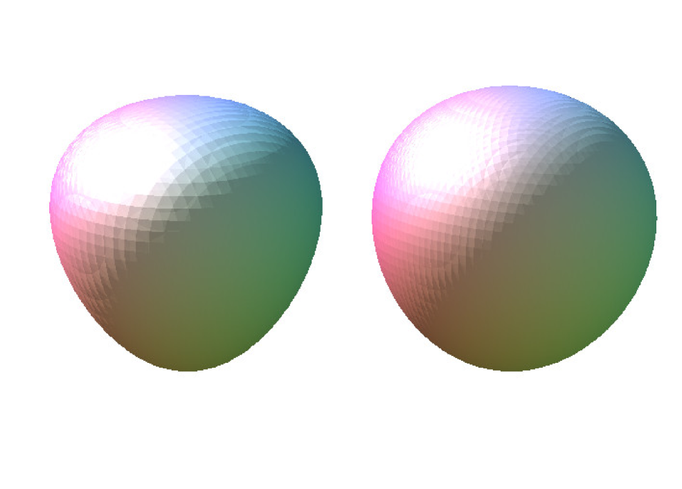
Figure 1: (Color online) The detector profile. Left: an accelerated observer, with the acceleration being taken as, $a=5\cdot 10^{26}\rm m/s^{2}$. Right: an inertial observer ($a=0$).

Performing the integration, we obtain,

$$\gamma(\tau)= \frac{2\lambda^{2}}{\pi^{2}}\Re\ln(1+{i\tau}/l)$$

$$-\frac{4\lambda^{2}}{\pi^{2}}\Re\ln\bigg{(}\frac{\Gamma(1+al/2\pi+ia\tau/2\pi)}{\Gamma(1+al/2\pi)}\bigg{)},$$ (15)

where $\Gamma(z)$ is the Gamma-function.

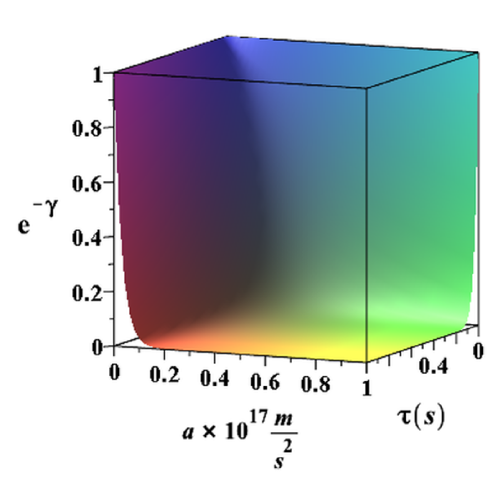
Figure 2: (Color online) The exponential decay function, $e^{-\gamma(\tau)}$ vs $\tau$ and $a$ ($\lambda=10^{-3}$).

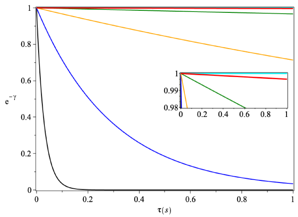
Figure 3: (Color online) The exponential decay function, $e^{-\gamma(\tau)}$ vs $\tau$ ($\lambda=10^{-3}$). From the top to the bottom: $a=0$ (cyan), $a=10^{13}\rm m/s^{2}$ (red), $a=10^{14}\rm m/s^{2}$ (green), $a=10^{15}\rm m/s^{2}$ (orange), $a=10^{16}\rm m/s^{2}$ (blue), $a=10^{17}\rm m/s^{2}$ (black). Inset: zoom of the main figure.

Returning to the physical units, we find that in the limit of $a\tau/2\pi c\gg 1$, one can approximate the decoherence function as,

$$\gamma(\tau)\approx\frac{2\lambda^{2}}{\pi^{2}}\ln(c\tau/l)+\frac{\lambda^{2}a\tau}{\pi^{2}c}.$$ (16)

As one can see, the detector exhibits the full phase decoherence, even for an inertial motion. However, the decay process is very slow, $\gamma\propto\ln\tau$. In the limit of large accelerations, one can neglect the contribution of the first term in Eq. (16), and recast the decoherence function as, $\gamma(\tau)\approx\Gamma_{d}\tau$, where $\Gamma_{d}=\lambda^{2}a/(\pi^{2}c)$ denotes the decoherence decay rate. We conclude that the decoherence effect is insensitive to the choice of the cutoff and is highly sensitive to the choice of the coupling constant, $\lambda$.

In Figs. 2, and 3, we present the results of numerical simulations for the trial coupling constant, $\lambda=10^{-3}$. In Fig. 2, the exponential decay function is depicted as a function of the acceleration and proper time of the accelerating observer. In Fig. 3, we plot the exponential decay function as a function of time and for different choices of the acceleration: $a=0$, $a=10^{13}\rm m/s^{2}$, $a=10^{14}\rm m/s^{2}$, $a=10^{15}\rm m/s^{2}$, $a=10^{16}\rm m/s^{2}$ and $a=10^{17}\rm m/s^{2}$.

Setup for the Gedanken experiment. – We consider two identical detectors coupled to the scalar field in both inertial and accelerated reference frames. The experiment consists of comparing the decoherence for inertial and accelerated observers.

Let us denote by $\sigma$ the magnitude of the decoherence function that can be measured in the experiment. Then, the time required to make the measurement, can be estimated as follows: $\tau_{i}\approx(l/c)\exp(\pi^{2}\sigma/\lambda^{2})$ for the detector at rest in Minkowski space, and $\tau_{a}=\sigma/\Gamma_{d}$ for the uniformly accelerated detector. By choosing, $\sigma=10^{-4}$, we find $\tau_{i}\sim e^{10^{3}}\,\rm s$, and $\tau_{a}\approx 3\cdot 10^{11}/a\,[\rm s]$. Then, for the acceleration, $a=10^{13}\rm m/s^{2}$, we obtain, $\tau_{a}\approx 30\,\rm ms$, and $\tau_{a}\approx 3\,\rm\mu s$ for $a=10^{17}\rm m/s^{2}$.

Laboratory bounds. – Due to the Lorentz contraction of time, for the high accelerations, one might expect a significant difference between the decoherence time for the accelerated observer and for the inertial one. Indeed, while for non-relativistic velocities, the observation time in the laboratory system is, $\Delta t\approx\tau$, where $\tau$ denotes the decoherence time for the accelerated observer, for the ultra-relativistic motion, one might expect, $\Delta t\gg\tau$. This imposes strong restrictions on the upper limit of the observation time in the Rindler spacetime.

For definiteness, let us consider two cases: (1) non-relativistic motion with $v\lesssim 0.2\,c$; (2) ultra-relativistic motion with $v\lesssim 0.95\,c$. In the first case, we obtain: $\Delta t_{1}\approx\tau_{1}$, and $\tau_{1}\lesssim 0.2c/a$. In the second case, we find: $\Delta t_{2}\approx 1.8\tau_{2}$ and $\tau_{2}\lesssim 2c/a$. Substituting $\tau_{1,2}$ in Eq. (16), we obtain $\gamma(\tau_{1})\approx 0.02{\lambda^{2}}$, and $\gamma(\tau_{2})\approx 0.2{\lambda^{2}}$.

Concluding remarks. – We demonstrated that the information about the presence of the Unruh effects is encoded in the decoherence - the exponential decay of the non-diagonal elements of the reduced density matrix. The phase decay of the reduced density matrix can be observable for the accelerations as low as $10^{13}\,\rm m/s^{2}$. Such accelerations should be sustained only for a time $\approx 100\,\mu s$.

Our approach has the limitations related to the decoherence observation time from the perspective of an inertial observer at rest, in the Minkowski spacetime. Note, that the same restrictions are valid for any detector based on the indirect measurement of the Unruh effect.

Appendix A Supplemental material

A.1 Evolution operator

To proceed with calculations of evolution operator, we use the interaction picture writing the interaction Hamiltonian as,

$$H_{I}(\tau)=e^{-iH_{f}\tau}H_{sd}e^{iH_{f}\tau},$$ (17)

where $H_{f}=\mbox{$1{\bf l}$}\otimes\sum_{\omega>0}\sum_{\textbf{k}_{\bot}}\omega b^{\dagger}_{\mathbf{k}}b_{\mathbf{k}}$ and,

$$H_{sd}={{\varepsilon}\over{2}}\sigma_{z}\otimes\mbox{$1{\bf l}$}+\frac{\lambda}{\sqrt{V}}\sigma_{z}\otimes\sum_{\omega>0}\sum_{\textbf{k}_{\bot}}\frac{1}{\sqrt{2\omega}}(g_{\mathbf{k}}b^{\dagger}_{\mathbf{k}}+g^{\ast}_{\mathbf{k}}b_{\mathbf{k}}).$$ (18)

Then, in the interaction picture, the evolution operator, $U(\tau)=\hat{T}\exp\Big{(}-{i}\int_{0}^{\tau}dt^{\prime}H_{I}(t^{\prime})\Big{)}$, can be written as G. P. Berman, D. I. Kamenev and V. I. Tsifrinovich (2005),

$$U(\tau)=\exp\Big{(}-i\nu(\tau)\mbox{$1{\bf l}$}+i\frac{\varepsilon}{2}\sigma_{z}\otimes\mbox{$1{\bf l}$}+\sigma_{z}\otimes\sum_{{\mathbf{k}}}(b^{\dagger}_{\mathbf{k}}\xi_{\mathbf{k}}(\tau)-b_{\mathbf{k}}\xi^{\ast}_{\mathbf{k}}(\tau))\Big{)},$$ (19)

where,

$$\nu(\tau)=\frac{i}{2}\sum_{{\mathbf{k}}}\int^{\tau}_{0}\big{(}\xi^{\ast}_{\mathbf{k}}(t)\dot{\xi}_{\mathbf{k}}(t)-\xi_{\mathbf{k}}(t)\dot{\xi}^{\ast}_{\mathbf{k}}(t)\big{)}dt,\quad\xi_{\mathbf{k}}(\tau)=\lambda g_{\mathbf{k}}\frac{1-e^{-i\omega\tau}}{\sqrt{2V}\omega^{3/2}}.$$ (20)

The results of the action of the evolution operator (19) on an arbitrary pure initial state of the entire system, can be described by the expressions,

$$U(\tau)|\downarrow\rangle\otimes|\psi_{F}\rangle= e^{-i\nu(\tau)-i\varepsilon\tau/2}|\downarrow\rangle\otimes\prod_{k}D\Big{(}-\xi_{\mathbf{k}}(\tau)\Big{)}|\psi_{F}\rangle,$$ (21)

$$U(\tau)|\uparrow\rangle\otimes|\psi_{F}\rangle= e^{-i\nu(\tau)+i\varepsilon\tau/2}|\uparrow\rangle\otimes\prod_{k}D\Big{(}\xi_{\mathbf{k}}(\tau)\Big{)}|\psi_{F}\rangle,$$ (22)

where $|\psi_{F}\rangle$ is an initial state of the scalar field, and $D(\xi_{\mathbf{k}})$ denotes the displacement operator M. Hillery (1984):

$$D(\xi_{\mathbf{k}})=e^{\xi_{\mathbf{k}}b^{\dagger}_{\mathbf{k}}-\xi^{\ast}_{\mathbf{k}}b_{\mathbf{k}}}.$$ (23)

The density operator, $\varrho(\tau)$, for the entire system, at time $\tau=\tau_{0}$, is taken in the form, $\varrho(\tau_{0})=|\Psi_{0}\rangle\langle\Psi_{0}|$. Here, $|\Psi_{0}\rangle=|\psi_{0}\rangle\otimes|0_{M}\rangle$. The wave function, $|\psi_{0}\rangle$, denotes the initial state of the detector, and $|0_{M}\rangle$ stands for the Minkowski vacuum. The reduced density matrix of the detector, $\rho(\tau)$, is obtained by tracing out all scalar field degrees of freedom. Its matrix elements are given by,

$$\rho_{ij}(\tau)=\langle i|{\rm Tr}_{R}U(\tau)\varrho(\tau_{0})U^{-1}(\tau)|j\rangle,\quad(i,j=0,1),$$ (24)

where the index $i=0$ is associated with the eigenvector $|\downarrow\rangle$ and the index $i=1$ is associated with the eigenvector $|\uparrow\rangle$. Using Eqs. (21) and (22), one can show that $\rho_{00}(\tau)=\rho_{00}(\tau_{0})$, $\rho_{11}(\tau)=\rho_{11}(\tau_{0}),$ and,

$$\rho_{01}(\tau)=e^{i\varepsilon\tau-\gamma(\tau)}\rho_{01}(\tau_{0}).$$ (25)

A.2 Bogolyubov transformations

The relations between the creation and annihilation operators in the Rindler spacetime and in the Minkowski spacetime are determined by the Bogolyubov transformations: $\hat{b}_{k}=\sum_{p}(\alpha_{{\mathbf{k}}{\mathbf{p}}}\hat{a}_{\mathbf{p}}-\beta^{\ast}_{{\mathbf{k}}{\mathbf{p}}}\hat{a}^{\dagger}_{\mathbf{p}})$. Note that, while the operators $\hat{b}_{\mathbf{k}}$ annihilate the Rindler vacuum, $|0_{R}\rangle$, the operators $\hat{a}_{\mathbf{p}}$ annihilate the Minkowski vacuum, $|0_{M}\rangle$. The computation of the Bogolyubov coefficients yields L. C. B. Crispino, A. Higuchi and G. E. A. Matsas (2008):

$$\hat{b}_{\omega\mathrm{k}_{\perp}}=\frac{\hat{a}_{-\omega\mathbf{k}_{\perp}}+e^{-\pi\omega/a}\hat{a}_{\omega-\mathbf{k}_{\perp}}^{\dagger}}{\sqrt{1-e^{-2\pi\omega/a}}}.$$ (26)

Using the Bogolyubov transformations, one can easily calculate the mean number of the particles in the mode $\omega$:

$$\bar{n}_{\omega}=\langle 0_{M}|b^{\dagger}_{\mathbf{k}}b_{\mathbf{k}}|0_{M}\rangle=\frac{1}{e^{2\pi\omega/a}-1}.$$ (27)

In order to obtain the decoherence function, $\gamma(\tau)$, we employ the Bogolyubov transformations. Substituting (26) in Eq. (23) and using Eqs. (21), (22) and (24), after some algebra we obtain,

$$\gamma(\tau)={2}\sum_{{\mathbf{k}}}|\xi_{k}(\tau)|^{2}(1+2\bar{n}_{k})={2}\sum_{{\mathbf{k}}}|\xi_{k}(\tau)|^{2}\coth\Big{(}\frac{\pi\omega_{k}}{a}\Big{)}.$$ (28)

In the continuous limit, the sum over ${\mathbf{k}}$ is replaced by the integral, $\sum\rightarrow V/(2\pi)^{3}\int d^{3}{\mathbf{k}}$, and the decoherence function is defined by the integral:

$$\gamma(\tau)=\frac{\lambda^{2}}{4\pi^{3}}\int_{0}^{\infty}\frac{|g_{\omega}|^{2}}{\omega}{\rm sinc}^{2}\Big{(}\frac{\omega\tau}{2}\Big{)}\coth\Big{(}\frac{\pi\omega}{a}\Big{)}d\omega,$$ (29)

where, $|g_{\omega}|^{2}=\int|g_{\mathbf{k}}|^{2}d^{2}{\mathbf{k}}_{\perp}$ and ${\rm sinc}(x)=\sin(x)/x$.