Individual-Level Modelling of Infectious Disease Data: EpiILM

Abstract

In this article we introduce the R package EpiILM, which provides tools for simulation from, and inference for, discrete-time individual-level models of infectious disease transmission proposed by Deardon et al. (2010). The inference is set in a Bayesian framework and is carried out via Metropolis-Hastings Markov chain Monte Carlo (MCMC). For its fast implementation, key functions are coded in Fortran. Both spatial and contact network models are implemented in the package and can be set in either susceptible-infected (SI) or susceptible-infected-removed (SIR) compartmental frameworks. Use of the package is demonstrated through examples involving both simulated and real data.

Introduction

The task of modelling infectious disease transmission through a population poses a number of challenges. One challenge is that successfully modelling many, if not most, infectious disease systems requires accounting for complex heterogeneities within the population. These heterogeneities may be characterized by individual-level covariates, spatial clustering, or the existence of complex contact networks through which the disease may propagate. A second challenge is that there are inherent dependencies in infection (or event) times.

To model such scenarios, Deardon et al. (2010) introduced a class of discrete time individual-level models (ILMs), fitting the models to data in a Bayesian Markov chain Monte Carlo (MCMC) framework. They applied spatial ILMs to the UK foot-and-mouth disease (FMD) epidemic of 2001, which accounted for farm-level covariates such as the number and type of animals on each farm. However, the ILM class also allows for the incorporation of contact networks through which disease can spread. Once fitted, such models can be used to predict the course of an epidemic (e.g., O’Reilly et al., 2018) or test the effectiveness of various control strategies (e.g., Tildesley et al., 2006) that can be imposed upon epidemics simulated from the fitted model.

A third challenge when modelling disease systems is that very little software so far has been made available that allows for simulation from, and especially inference for, individual-level models of disease transmission. Most inference for such models is carried out in fast, low-level languages such as Fortran or variants of C, which makes it difficult for researchers (e.g., public health epidemiologists) without a strong background in computational statistics and programming to make use of the models.

A number of R packages have recently been developed for modelling infectious disease systems (e.g., R0 (Boelle and Obadia, 2015), EpiEstim (Cori, 2019), EpiModel (Jenness et al., 2018), and epinet (Groendyke and Welch, 2016)). Most of these packages can be used to carry out epidemic simulation from given models; in addition, R0 or EpiEstim, for example, can be used to calculate the (basic) reproduction number under various scenarios. The EpiModel package allows for the simulation of epidemics from stochastic models, primarily exponential-family random graph models (ERGMs), and provides tools for analyzing simulation output. Functions for carrying out some limited forms of inference are also provided. Another widely used package for monitoring and modelling infectious disease spread through surveillance data is surveillance (Meyer et al., 2017). This package provides for a highly flexible modelling framework for such data. However, the package does not cover mechanistic, individual-level disease transmission models such as those of Deardon et al. (2010).

Here, we detail a novel R statistical software package EpiILM for simulating from, and carrying out Bayesian MCMC-based statistical inference for spatial and/or network-based models in the Deardon et al. (2010) individual-level modelling framework. The package allows for the incorporation of individual-level susceptibility and transmissibility covariates in models, provides various methods of summarizing epidemic data sets, and permits reasonably involved scenarios to be coded up by the user due to its setting in an R framework. The main functions, including for likelihood calculation are coded in Fortran in order to achieve the goal of agile implementation.

The type of spatial and network-based transmission models that EpiILM facilitates can be used to model a wide range of disease systems, as well as other transmissible processes. Human diseases such as influenza, measles or HIV, tend to be transmitted via interactions which can be captured by contact networks. For example, Malik et al. (2014) used a network representing whether two people shared the same household for modelling influenza spread in Hong Kong. Networks can also be used to characterize social or sexual relationships.

In the livestock industries, diseases are often transmitted from farm to farm via supply trucks or animal movements from farm to farm, or from farm to market. For example, ILM’s were used by Kwong et al. (2013) to model the spread of porcine reproductive and respiratory syndrome (PRRS) through Ontario swine farms via such mechanisms. Spatial mechanisms are also often important in livestock industries (e.g., Jewell et al., 2009; Deardon et al., 2010; Kwong et al., 2013), as well as for modelling crop diseases (e.g., Pokharel and Deardon, 2016), since airborne spread is often a key factor.

Further, these types of models can also be used to model transmissible processes other than infectious disease spread. For example, Cook et al. (2007) used similar models to model the transmission of alien species through a landscape; specifically, giant hogweed in the UK. In addition, Vrbik et al. (2012) used spatial ILM’s to model fire spread. They looked at fire spread under controlled conditions, but such models would likely be useful for modelling the spread of forest fires since important covariates such as vegetation-type could be incorporated into the models.

Data from infectious disease systems are generally ’time-to-event’, typically involving multiple states. However, standard survival models (e.g., Cox (1972), Therneau (2015)) or multi-state time-to-event models (e.g., see Jackson (2011)) are not applicable here, because in an infectious disease system individual event times cannot be assumed independent even after conditioning on covariates. That is, my risk of contracting and infectious disease generally depends upon the disease state of other individuals in the population; this is not typically the case for most cancers, for example to which more standard models can be applied.

The remainder of this paper is structured as follows: Section 2 explains the relevant models involved in the package; Section 3 describes the contents of the package along with some illustrative examples; and Section 4 concludes the paper with a brief discussion on future development.

Model

In our EpiILM package, we consider two compartmental frameworks: susceptible-infectious (SI) and susceptible-infectious-removed (SIR). In the former framework, individuals begin in the susceptible state (S) and if/when infected become immediately infectious (I) and remain in that state indefinitely. In the latter framework, individuals once infected remain infectious for some time interval before entering the removed state (R). This final state might represent death, quarantine, or recovery accompanied by immunity. We consider discrete time scenarios so a complete epidemic history is represented by $t=1,2,\dots,t_{end}$, where (typically) $t=1$ is the time when the first infection is observed and $t_{end}$ is the time when the epidemic ends. Hence, for a given time point $t$, an individual $i$ belongs to one, and only one, of the sets $S(t)$ or $I(t)$ if the compartmental framework is SI, and $i$ belongs to one, and only one, of the sets $S(t)$, $I(t)$, or $R(t)$ if the compartmental framework is SIR.

Under either framework, the probability that a susceptible individual $i$ is infected at time point $t$ is given by $\mathop{\operator@font IP\hskip 0.13pt}(i,t)$ as follows:

$$\mathop{\operator@font IP\hskip 0.13pt}(i,t)=1-\exp\{-\Omega_{S}(i)\sum_{j\in I(t)}{\Omega_{T}(j)\kappa(ij)}-\varepsilon\},\hskip 5.69046pt\Omega_{S}(i)>0,\hskip 2.84544pt\Omega_{T}(j)>0,\hskip 2.84544pt\varepsilon>0$$ (1)

where: $\Omega_{S}(i)$ is a susceptibility function that accommodates potential risk factors associated with susceptible individual $i$ contracting the disease; $\Omega_{T}(j)$ is a transmissibility function that accommodates potential risk factors associated with infectious individual $j$ contracting the disease; $\varepsilon$ is a sparks term which represents infections originating from outside the population being observed or some other unobserved infection mechanism; and $\kappa(i,j)$ is an infection kernel function that represents the shared risk factors between pairs of infectious and susceptible individuals.

The susceptibility function can incorporate any individual-level covariates of interest, such as age, genetic factors, vaccination status, and so on. In Equation (1), $\Omega_{S}(i)$ is treated as a linear function of the covariates, i.e., $\Omega_{S}(i)=\alpha_{0}+\alpha_{1}X_{1}(i)+\alpha_{2}X_{2}(i)+\dots+\alpha_{n_{s}}X_{n_{s}}(i)$, where $X_{1}(i),\dots,X_{n_{s}}(i)$ denote $n_{s}$ covariates associated with susceptible individual $i$, along with susceptibility parameters $\alpha_{0},\dots,\alpha_{n_{s}}>0$. Note that, if the model does not contain any susceptibility covariates then $\Omega_{S}(i)=\alpha_{0}$ is used. In a similar way, the transmissibility function in Equation (1) can incorporate any individual-level covariates of interest associated with infectious individual. $\Omega_{T}(j)$ is also treated as a linear function of the covariates, but without the intercept term, i.e., $\Omega_{T}(j)=\phi_{1}X_{1}(j)+\phi_{2}X_{2}(j)+\dots+\phi_{n_{t}}X_{n_{t}}(j)$, where $X_{1}(j),\dots,X_{n_{t}}(j)$ denote the $n_{t}$ covariates associated with infectious individual $j$, along with transmissibility parameters $\phi_{1},\dots,\phi_{n_{t}}>0$. Also note that if the model does not contain any transmissibility covariates then $\Omega_{T}(j)=1$ is used.

In this package, we also consider two broad types of ILM models based on the type of the kernel function $\kappa(i,j)$: spatial and network-based ILMs. In the spatial-based ILMs, the infection kernel function is represented by the power-law function as

$$\kappa(ij)=d_{ij}^{-\beta},$$

where $\beta$ is the spatial parameter that accounts for the varying risk of transmitting disease over the Euclidean distance between individuals $i$ and $j$, $d_{ij}$. Whereas in the network-based ILMs, $\kappa(i,j)$ can be represented by one or more contact network matrices and is written as

$$\kappa(ij)=\beta_{1}\hskip 2.84544ptC^{(1)}_{ij}+\dots+\beta_{n}\hskip 2.84544ptC^{(n)}_{ij},$$

where $C^{(.)}_{ij}$ denotes the $(i,j)^{th}$ element of what we term the contact matrix of a given contact network; in graph theory this is more typically referred to as a (weighted) adjacency matrix. The corresponding $\beta_{(.)}$’s represent the effect of each of the $n$ networks on transmission risk. In each contact network, each individual in the population is denoted by a node and is connected by lines or edges. These connections represent potential transmission routes through which disease can spread between individuals in the population. If the network is unweighted, the contact matrix is treated as binary (0 or 1). If the edges have weights assigned to them, then $C^{(.)}_{ij}\in R^{+}$ or $C^{(.)}_{ij}\in[0,1]$ are typically used. These weights can be used to allow for different infection potential between different pairs of individuals. If the network is undirected, the contact matrix will be symmetric; if directed, it can be non-symmetric. Finally, the $C_{ii}$ (diagonal terms) are not used in the models and are typically set to $C_{ii}=0,\forall\hskip 1.42271pti.$

Note that $\mathop{\operator@font IP\hskip 0.13pt}(i,t)$ gives the probability that susceptible individual $i$ is infected at time point $t$, representing some interval in continuous time (e.g., a day or week), but they actually become infectious at time $t+1$.

Following Deardon et al. (2015), the likelihood function for the ILMs (1) is given by

$$f(S,I,R|\theta)=\prod_{t=1}^{t_{max}}f_{t}(S,I,R|\theta)$$ (2)

where

$$f_{t}(S,I,R|\theta)=\bigg{[}\prod_{i\in I(t+1)\backslash I(t)}\mathop{\operator@font IP\hskip 0.13pt}(i,t)\bigg{]}\bigg{[}\prod_{i\in S(t+1)}(1-\mathop{\operator@font IP\hskip 0.13pt}(i,t))\bigg{]}$$ (3)

and where, $\theta$ is the vector of unknown parameters, $I(t+1)\backslash I(t)$ denotes all new infections observed at $t+1$ in the infectious state at time $t$, and $t_{max}\leq t_{end}$ is the last time point at which data are observed or being simulated.

Contents of EpiILM

The EpiILM package makes use of Fortran code that is called from within R. This package can be used to carry out simulation of epidemics, calculate the basic reproduction number, plot various epidemic summary graphics, calculate the log-likelihood, and carry out Bayesian inference using Metropolis-Hastings MCMC for a given data set and model. The functions involved in the package are summarized in Table 1.

Function	Output
epiBR0	Calculates the basic reproduction number for a specified SIR model
epidata	Simulates epidemic for the specified model type and parameters
plot.epidata	Produces spatial plots of epidemic progression over time as well as various epidemic curves of epidata object
epidic	Computes the deviance information criterion for a specified individual-level model
epilike	Calculates the log-likelihood for the specified model and data set
epimcmc	Runs an MCMC algorithm for the estimation of specified model parameters
summary.mcmc	Produces the summary of epimcmc object
plot.mcmc	Plots epimcmc object
pred.epi	Computes posterior predictions for a specified epidemic model
plot.pred.epi	Plot posterior predictions

Table 1: Description of functions and their output in the EpiILM package

Simulation of epidemics

The function epidata() allows the user to simulate epidemics under different models and scenarios. One can use the argument type to select the compartmental framework (SI or SIR) and population size through the argument n. If the compartmental framework is SIR, the infectious period is passed through the argument infperiod. Depending on whether a spatial or network model is being considered, the user can pass the arguments: x, y for location and contact for contact networks. Users can also control the susceptibility function $\Omega_{S}(i)$ through the Sformula argument, with individual-level covariate information passable through this argument. If there is no covariate information, Sformula is null. An expression of the form Sformula = $\sim$ model is used to specify the covariate information, separated by + and - operators similar to the R generic function formula(). For example, $\Omega_{S}(i)=\alpha_{0}+\alpha_{1}X(i),\hskip 1.42271pti=1,\dots,n$ can be passed through the argument Sformula as Sformula = $\sim$ 1 + X. In a similar way, the user can control the transmissibility function $\Omega_{T}(i)$ through the Tformula argument. Note that, the Tformula must not include the intercept term to avoid model identifiability issues, i.e., for a model with one transmissibility covariate (X), the Tformula becomes Tformula = $\sim$ -1 + X. The spatial (or network), susceptibility, transmissibility, and spark (if any) parameters are passed through arguments beta, alpha, phi, and spark, respectively.

The argument tmin helps to fix the initial infection time while generating an epidemic. By default, tmin is set as time $t=1$. We can also specify the initial infective or infectives using the argument inftime. For example, in a population of $10$ individuals, we could choose, say, the third individual to become infected at time point 1, using the option inftime = c(0, 0, 1, 0, 0, 0, 0, 0, 0, 0). We could also infect more than one individual and they could be infected at different time points. This allows simulation from a model conditional on, say, data already observed, if we set the tmin option at the maximum value of inftime.

The output of the function epidata() is formed as class of epidata object. This epidata object contains a list that consist of type (the compartmental framework), XYcoordinates(the XY coordinates of individual for spatial model) or contact (the contact network matrix for the network model), inftime (the infection times) and remtime (the removal times). Other functions such as plot.epidata and epimcmc involved in the package use this object class as an input argument.

Descriptive analyses

We introduce an S3 method plot function to graphically summarize, and allow for a descriptive analyses of, epidemic data. The function plot.epidata() illustrate the spread of the epidemic over time. One of the key input arguments (x) of this function has to be an epidata object. The other key argument plottype has two options: curve and spatial. Specifying the first option produces various epidemic curves, while the latter show the epidemic propagation over time and space when the model is set to spatial-based. When the plottype = curve, an additional argument needs to be passed through the function through curvetype. This has four options: curvetype = "complete" produces curves of the number of susceptible, infected, and removed individuals over time (when type = "SIR’’); "susceptible" gives a single curve for the susceptible individuals over time; "totalinfect" gives the cumulative number of infected individuals over time; and "newinfect" produces a curve of the number of newly infected individuals at each time point.

The plot functions plot.epimcmc() and plot.pred.epi() can be used to illustrate inference results (see Bayesian inference section). Detailed explanation is provided in the corresponding subsections.

Example: spatial model

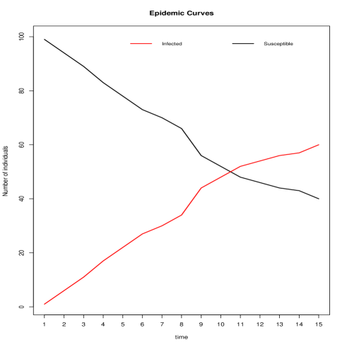
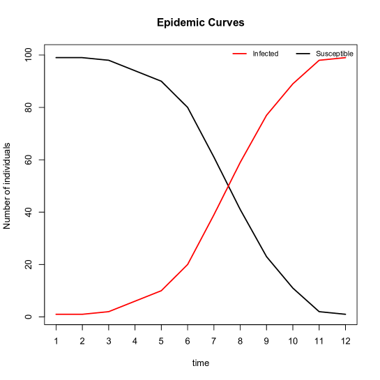
Suppose we want to simulate an epidemic from the model (1) using a spatial kernel with type SI, $\Omega_{s}(i)=\alpha$, and no transmissibility covariates, $\Omega_{T}(j)=1$. Choosing the infectivity parameter $\alpha=0.3$, spatial parameter $\beta=5.0$, sparks parameter $\varepsilon=0$, and $t_{max}=15$, the model is given by:

$$\mathop{\operator@font IP\hskip 0.13pt}(i,t)=1-\exp\{-0.3\sum_{j\in I(t)}{d_{ij}^{-5}}\},\hskip 2.84544ptt=1,\dots,15$$ (4)

where $d_{ij}$ is the Euclidean distance between individuals $i$ and $j$, with their locations specified through x and y.

First, we install the EpiILM package and call the library.

R> install.packages("EpiILM")R> library("EpiILM")Then, let us simulate (x, y) coordinates uniformly across a $10\times 10$ unit square.

R> x <- runif(100, 0, 10)R> y <- runif(100, 0, 10)One could now use the following syntax to simulate an epidemic from spatial model (4) and summarize the output as an epidemic curve and spatial plot.

R> SI.dis <- epidata(type = "SI", n = 100, tmax = 15, sus.par = 0.3, beta = 5.0,+                                x = x, y = y)R> SI.dis$inftime  [1]  0  0 10  4  7  0  0  0  4  5  0  0  9  2  6  6  3  0  0  0 11 [22]  0  0  9 12  3  0 15  9  0  8  0  0  0 11  9  0  2  0  5  7  0 [43]  2 15  7  0  0  5  0  0  0 14  8  2  0 15  9 10 10  4  1  5  4 [64]  6 11  3  0  8  0  6  8  5 12  4  2 13  0  9  3  6  3  4  9 13 [85]  0  0  0  0  0  0  0  0 10  0  9 11  9  9  0  0

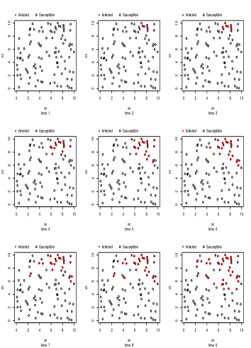
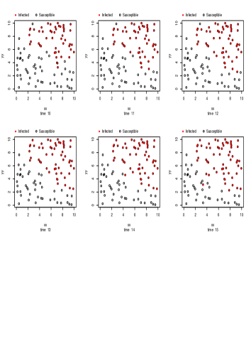
Here, the epidemic is generated across the uniformly distributed population of $100$ individuals with a default first infection time $t=1$ and last observed time point of $t_{max}=15$. The declaration of the spatial locations of individuals through x and y specifies that we are simulating from a spatial model. (See later for network-based models). The output SI.dis$\$$inftime provides the times at which individuals enter the infectious state, with $0$ representing individuals who are still susceptible at time $t_{max}$. Figures 1 and 2 show the summary graphics for the simulated epidemic, which are produced using the S3 method plot.epidata() as follows:

R> plot(SI.dis, plottype = "curve", curvetype ="complete")R> plot(SI.dis, plottype = "spatial")

Figure 1: Epidemic curves of simulated epidemic from (4) for 100 individuals at $t=1,\dots,15$

Figure 2: Simulated epidemic from (4) for 100 individuals, where open circles represent susceptible individuals and filled red circles represent infected individuals

Example: network model

To illustrate simulation from a contact network-based model, we consider a disease system in which disease transmission can occur through a single, directed, binary network over a population of $n=100$ individuals. The elements in the contact matrix represent the existence or non-existence of a directed connection through which disease can transmit between two individuals in the population. Each individual within the population is represented by a row and column within the matrix. Specifically, an element $C_{ij}$ in the contact matrix is given by:

$$C_{ij}=\left\{\begin{array}[]{l}1\hskip 14.22636pt\textrm{ if a directed edge exists between $i$ and $j$ }\\ 0\hskip 14.22636pt\textrm{ otherwise }\end{array}\right.$$ (5)

We also consider the inclusion of a binary susceptibility covariate $Z$ in the model. This can be thought to represent, say, treatment or vaccination status. The infection model is then given by

$$\mathop{\operator@font IP\hskip 0.13pt}(i,t)=1-\exp\{-(\alpha_{0}+\alpha_{1}Z_{i})\sum_{j\in I(t)}{C_{ij}}\},\hskip 2.84544ptt=1,\dots,t_{max}$$ (6)

where $\alpha_{0}$ is the baseline susceptibility and $\alpha_{1}$ is the binary treatment effect. The parameters in the model are set to be $(\alpha_{0},\alpha_{1})=(0.1,0.05)$ and $\varepsilon=0$, and we also set $t_{max}=15$. We simulate a directed network using the following code:

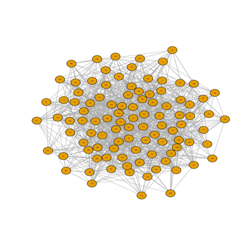
R> contact <- matrix(rbinom(10000, 1, 0.1), nrow = 100, ncol = 100)R> diag(contact[, ]) <- 0Various packages are available in R for network visualization, such as igraph, ergm, etc and as an example, we use the igraph package for the network display as shown in Figure 3.

R> require("igraph")R> net1 <- graph_from_adjacency_matrix(contact)R> plot(net1, vertex.size = 10, vertex.label.cex = 0.5, edge.arrow.mode = "-")

Figure 3: Contact network generated for model (6)

The epidemic is generated using the function epidata(). The arguments Sformula = $\sim$ Z and sus.par = c(0.1, 0.05) define the susceptibility function $0.1+0.05Z_{i}$. As there is one contact network matrix in the model, the effect of the network $C$ is set to one by default. The use of the contact argument informs the package that we are dealing with a contact network-based model.

R> Z <- round(runif(100, 0, 2))R> SI.contact <- epidata(type = "SI", Sformula = ~Z, n = 100, tmax = 15,+           sus.par = c(0.1, 0.05),  contact = contact)R> SI.contact$inftime  [1]  0  9 11 10  9  5  8  9  8  9  9 10  1  7 12 11  7 11  8  4  8 [22] 10  8 11  7  9 11  5  7  6  6  8  9  8  9  6  6  7  9  9  7  4 [43]  7 10  8  3 10  9 10 11  6  7  9  6  5 11  4  7  8  8 10  8  8 [64]  7  7  6 11  7  8  7  6  8  8 10  7  6 10 11  9  6 10  7  4  7 [85]  8  7  9  9 10  9  8 10  5  8  7  7  8  9  9  8Figure 4 shows the epidemic curve, obtained via the following code.

R> plot(SI.contact, plottype = "curve", curvetype ="complete")

Figure 4: Epidemic curve of contact network model (6) for 100 individuals

Bayesian Inference

In EpiILM, ILMs can be fitted to observed data within a Bayesian framework. A Metropolis-Hastings MCMC algorithm is provided which can be used to estimate the posterior distribution of the parameters. The function epimcmc() provides three choices for the marginal prior distribution of each parameter: the gamma, half-normal, and uniform distributions. The parameters are assumed to be a priori independent. The proposal used is a Gaussian random walk. Again, users can use the Sformula and Tformula arguments to specify any individual-level susceptibility and transmissibility covariates. Users can also control the number of MCMC simulations, initial values, and proposal variances of the parameters to be estimated. Note that in case of fixing one parameter and updating other parameters, users can do it by setting the proposal variance of fixed parameter to zero. This is usually the case to avoid identifiability issue when the model has both susceptibility and transmissibility covariates without intercept terms. Again, spatial/network, susceptibility parameters and transmissibility parameters are passed through arguments beta, sus.par and trans.par, respectively. One can specify the spark parameter using the spark argument, but by default its value is $0$. epimcmc() can also call the adaptive MCMC method of inference facilitated by the adaptMCMC package. Specifically, users can pass the argument adapt = TRUE along with acc.rate to run the adapt MCMC algorithm.

We can use the S3 method functions summary.epimcmc() and plot.epimcmc() available in the package for output analysis and diagnostics. Both are dependent upon the coda package. The argument plottype in the function plot.epimcmc, has two options to specify which samples are to be plotted: (1) "parameter" is used to produce trace plots (time series plots) of the posterior distributions of the model parameters, and (2) "loglik" to produce trace plots of the log likelihood values of the model parameter samples. Other options that are used in the coda package can be used in the plot.epimcmc() as well; e.g., start, end, thin, density, etc.

Spatial or network-based ILMs can be fitted to data as shown in the following examples.

Example: spatial model

Suppose we are interested in modelling the spread of a highly transmissible disease through a series of farms, say $n=100,$ along with an assumption that the spatial locations of the farms and the number of animals on each farm are known. In this situation, it is reasonable to treat the farms themselves as individual units. If we treat the extent of infection from outside the observed population of farms as negligible ($\varepsilon=0$), we can write the ILM model as

$$\mathop{\operator@font IP\hskip 0.13pt}(i,t)=1-\exp\{-(\alpha_{0}+\alpha_{1}A(i))\sum_{j\in I(t)}{d_{ij}^{-\beta}}\},\hskip 2.84544ptt=1,\dots,t_{max},$$ (7)

where the susceptibility covariate $A$ represents the number of animals on each farm, $\alpha_{0}$ is the baseline susceptibility, $\alpha_{1}$ is the number of animals effect, and $\beta$ is the spatial parameter. Let us use the same (simulated) spatial locations from the previous spatial model example and set the parameters $(\alpha_{0},\alpha_{1})=(0.2,0.1)$ and $\beta=5$. We also set $t_{max}=50$. Considering an SI compartmental framework for this situation, the epidemic is simulated using the following command:

R> A <- round(rexp(100,1/50))R> SI.dis.cov <- epidata(type = "SI", n = 100, tmax = 50, x = x, y = y,+                 Sformula = ~A, sus.par = c(0.2, 0.1), beta = 5)

We can now refit the generating model to this simulated data and consider the posterior estimates of the model parameters. We can do this using the following code:

R> t_end <- max(SI.dis.cov$inftime)R> unif_range <- matrix(c(0, 0, 10000, 10000), nrow = 2, ncol = 2)R> mcmcout_Model7 <- epimcmc(SI.dis.cov, Sformula = ~A, tmax = t_end, niter = 50000,+                      sus.par.ini = c(0.001, 0.001), beta.ini = 0.01,+                      pro.sus.var = c(0.01, 0.01), pro.beta.var = 0.5,+                      prior.sus.dist = c("uniform","uniform"), prior.sus.par = unif_range,+                      prior.beta.dist = "uniform", prior.beta.par = c(0, 10000))

where niter denotes the number of MCMC iterations and sus.par.ini and beta.ini are the initial values of the parameters to be estimated. The proposal variances for $(\alpha_{0},\alpha_{1})$ and $\beta$ are set to $(0.01,0.01)$ and $0.5$, respectively (after tuning). Vague uniform prior distributions are used for all three parameters, i.e., we choose $U(0,10000)$ for $\alpha_{0},\alpha_{1}$, and $\beta$. As the locations x and y are specified, a spatial ILM is fitted rather than a network-based ILM. Note that the full data set to which the model is being fitted consists of the spatial locations (x, y) and the infection times. Figure 5 displays the MCMC traceplot after 10000 burn-in using the command

R> plot(mcmcout_Model7, partype = "parameter", start = 10001, density = FALSE)

The posterior means and $95\%$ credible intervals (CI) of the parameters, calculated as the $2.5\%$ and $97.5\%$ percentiles of 50000 MCMC draws after a burn-in of 10000 iterations has been removed, can be obtained using the following code:

R> summary(mcmcout_Model7, start = 10001)Model: SI distance-based discrete-time ILMMethod: Markov chain Monte Carlo (MCMC)Iterations = 10001:50000Thinning interval = 1Number of chains = 1Sample size per chain = 400001. Empirical mean and standard deviation for each variable,   plus standard error of the mean:          Mean      SD  Naive SE Time-series SEalpha.1 0.2868 0.23516 0.0011758       0.012449alpha.2 0.1997 0.07544 0.0003772       0.002393beta.1  5.6790 0.48188 0.0024094       0.0146312. Quantiles for each variable:           2.5%    25%    50%    75%  97.5%alpha.1 0.02018 0.1141 0.2226 0.3917 0.9072alpha.2 0.08680 0.1486 0.1875 0.2395 0.3769beta.1  4.81361 5.3377 5.6704 5.9872 6.6588

Figure 5: MCMC traceplot for the estimation of model ( 7) parameters

Example: network model

Now consider modelling the spread of an animal infectious disease through a series of farms ($n=500$) in a region. We once again consider individuals in the population to be the farms, rather than animals themselves, and a single binary contact network to represent connections between farms. We assume that there are two species of animals in farms that play an important role in spreading the disease; let us say, cows and sheep. Thus, we include the number of cows and sheep on the farm as susceptibility and transmissibility covariates in the model. Thus, the probability of susceptible farm $i$ to be infected at time $t$ becomes:

$$\mathop{\operator@font IP\hskip 0.13pt}(i,t)=1-\exp\{-(\alpha_{1}X_{1}(i)+\alpha_{2}X_{2}(i))\sum_{j\in I(t)}{[\phi_{1}X_{1}(j)+\phi_{2}X_{2}(j)]C_{ij}}\},\hskip 2.84544ptt=1,\dots,t_{max}$$ (8)

with susceptibility parameters, ($\alpha_{1},\alpha_{2}$), transmissibility parameters, ($\phi_{1},\phi_{2}$), and $X_{1}$ and $X_{2}$ represent the number of sheep and cows in farms, respectively. Note, when we have a single network, there is no network parameter to estimate; this is to avoid problems of non-identifiability.

We can generate such a directed contact network using the following commands:

R> n <- 500R> contact <- matrix(rbinom(n*n, size = 1, prob = 0.1), nrow = n, ncol = n)R> diag(contact) <- 0

We also sample the number of sheep and cows on each farm using the following code

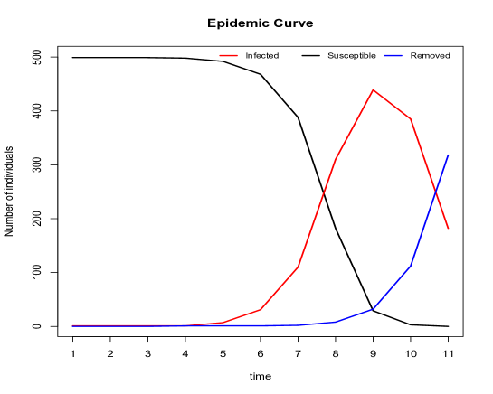
R> X1 <- round(rexp(n, 1/100))R> X2 <- round(rgamma(n, 50, 0.5))Assuming each infected farm to be infectious for an infectious period of 3 days and by setting $t_{max}=25$, $\alpha_{1}=0.003$, $\alpha_{2}=0.01$, $\phi_{1}=0.0003$, and $\phi_{2}=0.0002$, we can simulate the epidemic from the SIR network-based ILMs (8) as follows and the epidemic curves are shown in Figure 6.

R> infp <- rep(3, n)R>  SIR.net <- epidata(type = "SIR", n = 500, tmax = 15,+              sus.par = c(0.003, 0.01), trans.par = c(0.0003, 0.0002),+              contact = contact, infperiod = infp,+              Sformula = ~ -1 + X1 + X2, Tformula = ~ -1 + X1 + X2)R> plot(SIR.net, plottype = "curve", curvetype = "complete")

Figure 6: Epidemic curve of the contact network model (8) for 500 farms

To estimate the unknown parameters ($\alpha_{1}$, $\alpha_{2}$, $\phi_{1}$, $\phi_{2}$), we use the function epimcmc() assuming the event times (infection and removal times) and contact network are observed. Note that the specification of the contact argument means a network-based (rather than spatial) ILM will be assumed. We run the epimcmc() function to produce an MCMC chain of 50000 iterations assigning gamma prior distribution for the model parameters ($\alpha_{2}$, $\phi_{1}$, $\phi_{2}$) while fixing $\alpha_{1}$ to avoid the non-identifiablity issue in the model. This is done by setting the proposal variance of this parameter to zero in the pro.sus.var argument. To illustrate the use of adaptMCMC method, we set adapt = TRUE and set the acceptance rate as 0.5 via acc.rate = 0.5. It should also be noted that we need to provide initial values and proposal variances of the parameters when we use the adaptive MCMC option in the epimcmc() function. The syntax is as follows:

R> t_end <- max(SIR.net$inftime)R> prior_par <- matrix(rep(1, 4), ncol = 2, nrow = 2)R> mcmcout_SIR.net <- epimcmc(SIR.net, tmax = t_end, niter = 50000,+              Sformula = ~-1 + X1 + X2, Tformula = ~-1 + X1 + X2,+              sus.par.ini = c(0.003, 0.001), trans.par.ini = c(0.01, 0.01),+              pro.sus.var = c(0.0, 0.1), pro.trans.var = c(0.05, 0.05),+              prior.sus.dist = c("gamma", "gamma"), prior.trans.dist = c("gamma", "gamma"),+              prior.sus.par = prior_par, prior.trans.par = prior_par,+              adapt = TRUE, acc.rate = 0.5)Figure 7 shows the MCMC traceplot for the 50000 iterations. The estimate of the posterior mean of the model parameters ($\alpha_{2}$, $\phi_{1}$, $\phi_{2}$) and their $95\%$ credible intervals, after 10000 iterations of burn-in have been removed are: $\hat{\alpha_{2}}=0.0094\hskip 2.84544pt(0.0051,0.0168)$, $\hat{\phi_{1}}=0.0004\hskip 2.84544pt(0.0002,0.0007)$, and $\hat{\phi_{1}}=0.0002\hskip 2.84544pt(0.00006,0.0003)$.

Figure 7: MCMC traceplot for the estimation of model (8) parameters.

R> summary(mcmcout_SIR.net, start = 10001)

Model: SIR network-based discrete-time ILMMethod: Markov chain Monte Carlo (MCMC)Iterations = 10001:50000Thinning interval = 1Number of chains = 1Sample size per chain = 400001. Empirical mean and standard deviation for each variable,   plus standard error of the mean:             Mean        SD  Naive SE Time-series SEalpha.2 0.0093899 0.0030070 1.504e-05      1.866e-04phi.1   0.0004123 0.0001218 6.089e-07      4.483e-06phi.2   0.0001851 0.0000732 3.660e-07      1.911e-062. Quantiles for each variable:             2.5%       25%       50%       75%     97.5%alpha.2 5.130e-03 0.0071826 0.0088076 0.0110550 0.0168404phi.1   2.123e-04 0.0003226 0.0004020 0.0004879 0.0006800phi.2   6.646e-05 0.0001322 0.0001763 0.0002299 0.0003463

Case Study: Tomato spotted wilt virus (TSWV) data

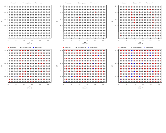
Here, we consider data from a field trial on TSWV as described in Hughes et al. (1997). The experiment was conducted on 520 pepper plants grown inside a greenhouse and the spread of the disease caused by TSWV was recorded at regular time intervals. Plants were placed in 26 rows spaced one metre apart, with 20 plants spaced half a metre apart in each row. The experiment started on May 26, 1993 and lasted until August 16, 1993. During this period, assessments were made every 14 days. We set the initial infection time to be $t=2$ as the epidemic starts at time point 2 and the last observation made is set to be $t=7$. The TSWV data in this package contain ID number, locations (x and y) and infectious and removal time of each individual. The data set was reconstructed from a spatial plot in Hughes et al. (1997). The infectious period for each tomato plant is assumed to span three time points (Brown et al., 2005, Pokharel and Deardon, 2016). Thus, an SIR model is fitted using the following code:

R> data(tswv)R> x <- tswv$xR> y <- tswv$yR> inftime <- tswv$inftimeR> removaltime <- tswv$removaltimeR> infperiod <- rep(3, length(x))In order to see the spatial dispersion of the TSWV data, we use the function epispatial(). As no new infections occurred at the second time point, we display spatial plots from that second observation by setting tmin = 2 (see Figure 8). The required code is given by:

R> epidat.tswv <- as.epidata(type = "SIR", n = 520, x = x, y = y,+                            inftime = inftime, infperiod = infperiod)R> plot(epidat.tswv, plottype = "spatial", tmin = 2)

Figure 8: Epidemic dispersion of TSWV data across a grid of 520 individuals, where open circles represent susceptible individuals, filled red circles represent infected individuals, and blue crosses represent the removed individuals.

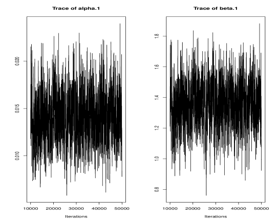
The function epimcmc() is used to fit our model to the data. We ran $50000$ MCMC iterations. The computing time taken for the MCMC is about 10 min on a 16 GB MacBook Pro with a 2.9 GHz Intel Core i5 processor. Proposal variances are chosen to be $0.000005$ and $0.005$ for $\alpha$ and $\beta$, respectively (after tuning). We use vague independent marginal prior distributions for the parameters. Here, a gamma distribution with shape parameter $1$ and rate parameter $10^{-3}$ is used for both $\alpha$ and $\beta$. We choose to fit our model to data starting at the second time point because no infections occur between the first and second time points. Thus, we again set tmin = 2. The code for fitting our model is:

R> mcmc.tswv <- epimcmc(epidat.tswv, tmin = 2, tmax = 10,+                niter = 50000, sus.par.ini = 0.0, beta.ini = 0.01,+               pro.sus.var = 0.000005, pro.beta.var = 0.005, prior.sus.dist = "gamma",+                prior.sus.par = c(1,10**(-3)), prior.beta.dist = "gamma",+                prior.beta.par = c(1,10**(-3)))The posterior mean estimates for this model are $\hat{\alpha}=0.014$ and $\hat{\beta}=1.351$. The $95\%$ credible interval of the posterior mean of $\alpha$ and $\beta$ are $(0.009,0.0190)$ and $(1.041,1.629)$, respectively. Once again, these intervals are calculated as the $2.5\%$ and $97.5\%$ percentiles of $50000$ draws after 10000 iterations of burn-in have been removed. The MCMC traceplots shown in Figure 9.

Figure 9: MCMC traceplots of the posterior samples for TSWV data

Conclusion

This paper discusses the implementation of the R software package EpiILM. Other than this package, there does not appear to be any R software that offers spatial and network-based individual-level modelling for infectious disease systems. Thus, this package will be helpful to many researchers and students in epidemiology as well as in statistics. These models can be used to model disease systems of humans (e.g., Malik et al. (2014)), animals (e.g., Kwong et al. (2013)), or plants (e.g., Pokharel and Deardon (2016)), as well as other transmission-based systems such as invasive species (e.g., Cook et al. (2007)) or fire spread (Vrbik et al., 2012).
The EpiILM package continues to exist as a work in progress. We hope to implement additional models and options in the future, that might be useful for other researchers in their research and teaching. Such additions may include the incorporation of time-varying networks, covariates and/or spatial kernels (e.g., Vrbik et al. (2012)), models that allow for a joint spatial and network-based infection kernel, uncertainty in the times of transitions between disease states (e.g., Malik et al. (2016)), unknown covariates (e.g., Deeth and Deardon (2013), and extensions to other compartmental frameworks such as SEIR and SIRS. Finally, we hope to extend the package to allow for the modelling of disease systems with multiple interacting strains or pathogens (Romanescu and Deardon, 2016).

Vineetha Warriyar. K. V.
Faculty of Veterinary Medicine
University of Calgary
Canada
vineethawarriyar.kod@ucalgary.ca

Waleed Almutiry
Department of Mathematics
College of Science and Arts in Ar Rass
Qassim University
Saudi Arabia
wkmtierie@qu.edu.sa

Rob Deardon
Faculty of Veterinary Medicine and Department of Mathematics and Statistics
University of Calgary
Canada
robert.deardon@ucalgary.ca

References

- Boelle and Obadia (2015) P.-Y. Boelle and T. Obadia. R0: Estimation of R0 and Real-Time Reproduction Number from Epidemics, 2015. URL https://CRAN.R-project.org/package=R0. R package version 1.2-6.
- Brown et al. (2005) S. Brown, A. Csinos, J. Díaz-Pérez, R. Gitaitis, S. LaHue, J. Lewis, N. Martinez, R. McPherson, S. Mullis, C. Nischwitz, et al. Tospoviruses in solanaceae and other crops in the coastal plain of georgia. The University of Georgia College of Agriculture and Environmental Sciences, Research Report, 704:19, 2005.
- Cook et al. (2007) A. R. Cook, G. Marion, A. Butler, and G. J. Gibson. Bayesian inference for the spatio-temporal invasion of alien species. Bulletin of Mathematical Biology, 69:2005–2025, 2007.
- Cori (2019) A. Cori. EpiEstim: Estimate Time Varying Reproduction Numbers from Epidemic Curves, 2019. URL https://CRAN.R-project.org/package=EpiEstim. R package version 2.2-1.
- Cox (1972) D. R. Cox. Regression models and life-tables. Journal of the Royal Statistical Society, 34(2):187–220, 1972.
- Deardon et al. (2010) R. Deardon, S. P. Brooks, B. T. Grenfell, M. J. Keeling, M. J. Tildesley, N. J. Savill, D. J. Shaw, and M. E. Woolhouse. Inference for individual-level models of infectious diseases in large populations. Statistica Sinica, 20(1):239, 2010.
- Deardon et al. (2015) R. Deardon, X. Fang, and G. Kwong. Statistical modeling of spatiotemporal infectious disease transmission. Analyzing and Modeling Spatial and Temporal Dynamics of Infectious Diseases (eds. Chen D, Moulin B, Wu J, pages 211–232, 2015.
- Deeth and Deardon (2013) L. Deeth and R. Deardon. Latent conditional individual-level models for infectious disease modeling. The International Journal of Biostatistics, 9(1):75–93, 2013.
- Groendyke and Welch (2016) C. Groendyke and D. Welch. epinet: Epidemic/Network-Related Tools, 2016. URL https://CRAN.R-project.org/package=epinet. R package version 2.1.7.
- Hughes et al. (1997) G. Hughes, N. McRoberts, L. V. Madden, and S. C. Nelson. Validating mathematical models of plant-disease progress in space and time. Mathematical Medicine and Biology, 14(2):85–112, 1997.
- Jackson (2011) C. H. Jackson. Multi-state models for panel data: The msm package for R. Journal of Statistical Software, 38(8):1–29, 2011. URL http://www.jstatsoft.org/v38/i08/.
- Jenness et al. (2018) S. Jenness, S. M. Goodreau, and M. Morris. EpiModel: Mathematical Modeling of Infectious Disease Dynamics, 2018. URL https://CRAN.R-project.org/package=EpiModel. R package version 1.6.1.
- Jewell et al. (2009) C. P. Jewell, T. Kypraios, P. Neal, and G. O. Roberts. Bayesian analysis for emerging infectious diseases. Bayesian Analysis, 4(4):465–496, 2009.
- Kwong et al. (2013) G. Kwong, Z. Poljak, R. Deardon, and C. Dewey. Bayesian analysis of risk factors for infection with a genotype of porcine reproductive and respiratory syndrome virus in ontario swine herds using monitoring data. Preventive Veterinary Medicine, 110(3-4):405–17, 2013.
- Malik et al. (2014) R. Malik, R. Deardon, G. Kwong, and B. J. Cowling. Individual-level modeling of the spread of influenza within households. Journal of Applied Statistics, 41(7):1578–1592, 2014.
- Malik et al. (2016) R. Malik, R. Deardon, and G. Kwong. Parameterizing spatial models of infectious disease transmission that incorporate infection time uncertainty using sampling- based likelihood approximations. PLoS One, 11(1), 2016. doi: 10.1371/journal.pone.0146253.
- Meyer et al. (2017) S. Meyer, L. Held, and M. Hohle. Spatio-temporal analysis of epidemic phenomena using the R package surveillance. Journal of Statistical Software, 77(11):1–55, 2017. doi: 10.18637/jss.v077.i11.
- O’Reilly et al. (2018) K. M. O’Reilly, R. Lowe, W. J. Edmunds, P. Mayaud, A. Kucharski, R. M. Eggo, S. Funk, D. Bhatia, K. Khan, M. U. G. Kraemer, A. Wilder-Smith, L. C. Rodrigues, P. Brasil, E. Massad, T. Jaenisch, S. Cauchemez, O. J. Brady, and L. Yakob. Projecting the end of the zika virus epidemic in latin america: a modelling analysis. BMC Medicine, 16(1):180, 2018.
- Pokharel and Deardon (2016) G. Pokharel and R. Deardon. Gaussian process emulators for spatial individual-level models of infectious disease. Canadian Journal of Statistics, 44(4):480–501, 2016.
- Romanescu and Deardon (2016) R. Romanescu and R. Deardon. Modelling two strains of disease via aggregate-level infectivity curves. Journal of Mathematical Biology, 72(5):1195–1224, 2016.
- Therneau (2015) T. M. Therneau. A Package for Survival Analysis in S, 2015. URL https://CRAN.R-project.org/package=survival. version 2.38.
- Tildesley et al. (2006) M. J. Tildesley, N. J. Savill, D. J. Shaw, R. Deardon, S. P. Brooks, M. E. J. Woolhouse, B. T. Grenfell, and M. J. Keeling. Optimal reactive vaccination strategies for an outbreak of foot-and-mouth disease in great britain. Nature, 440(7080):83–86, 2006.
- Vrbik et al. (2012) I. Vrbik, R. Deardon, Z. Feng, A. Gardner, and J. Braun. Using individual-level models to model the spatio-temporal dynamics of combustion. Bayesian Analysis, 7(3):615–638, 2012.