Analysis and applications of the residual varentropy of random lifetimes

Abstract

In reliability theory and survival analysis, the residual entropy is known as a measure suitable to describe the dynamic information content in stochastic systems conditional on survival. Aiming to analyze the variability of such information content, in this paper we introduce the variance of the residual lifetimes, “residual varentropy” in short. After a theoretical investigation of some properties of the residual varentropy, we illustrate certain applications related to the proportional hazards model and the first-passage times of an Ornstein-Uhlenbeck jump-diffusion process.

1 Introduction

The differential entropy is a well-known information measure that represents the expectation of the information content of an absolutely continuous random variable. The corresponding variance is termed varentropy and is used in various applications of information theory, such as for the estimation of the performance of optimal block-coding schemes. Recent contributions on the varentropy can be found in various papers by Arikan [1], Bobkov and Madiman [6], Fradelizi et al. [17], Kontoyiannis and Verdú [21], [22], [38]. Most of such results have been aimed to mathematical properties or to applications in information theory. However, it should be pointed out that such information measures often deserve interest in other fields, such as reliability and survival analysis. See, for instance, Nanda and Chowdhury [31] for a recent comprehensive review on the Shannon’s entropy and its applications in various fields. Several investigations have been oriented in the past to assess the information content of stochastic systems with special attention to dynamic measures related to the residual lifetime, the past lifetime, the inactivity time and their suitable generalizations. However, no efforts have been dedicated to the analysis of the variance of the information content in dynamic contexts.

On the ground of the above remarks, the motivation of this paper is to investigate the varentropy of residual lifetimes in a field related to reliability theory. The main aim is to measure the variability of the dynamic information content of stochastic systems that are conditioned on survival. This investigation is motivated by the need of constructing new mathematical tools suitable to describe the time course of the information content in addition to the residual entropy. Our attention is devoted to disclose properties of the varentropy of residual lifetimes. We give special attention to the conditions such that it is constant. We also discuss the effect of linear transformations and provide suitable lower and upper bounds. Moreover, we focus on certain applications involving the proportional hazards model and the first-passage times for Ornstein-Uhlenbeck jump-diffusion processes.

The paper is organized as follows: In Section 2, we recall some basic results on useful notions of information theory and reliability theory, with special attention to the varentropy and the residual lifetimes. In Section 3, we introduce the residual varentropy and investigate some properties of such new measure. Among other facts, we find conditions involving the generalized hazard rate such that the residual varentropy is constant, we discuss the effect of linear transformations, and obtain suitable upper and lower bounds for the residual varentropy. Section 4 is devoted to some applications. We first deal with the proportional hazard rates model and the reliability analysis of series system. We also discuss an application to first-passage times of the Ornstein-Uhlenbeck jump-diffusion process arising from the Ehrenfest model subject to catastrophes.

Throughout the paper, $\mathbb{E}[\,\cdot\,]$ denotes expectation, $g^{\prime}$ means the derivative of $g$, “$\log$” is the natural logarithm, and we set $0\log 0=0$ by convention. Moreover, notation $[X|B]$ is adopted for a random variable whose distribution is identical to that of $X$ conditional on $B$.

2 Background

Let $X$ be a random variable defined on a probability space $(\Omega,{\cal F},\mathbb{P})$, and let $F(t)=\mathbb{P}(X\leq t)$, $t\in\mathbb{R}$, be its cumulative distribution function (cdf). We denote by $\overline{F}(t)=1-F(t)$ the complementary distribution function, also known as survival function.

2.1 Varentropy

If $X$ is absolutely continuous with probability density function (pdf) $f(t)$, we can introduce the random variable

$$IC(X)=-\log f(X),$$ (1)

that is often referred as the (random) information content of $X$. We recall that $IC(X)$ is the natural counterpart of the number of bits needed to represent $X$ in the discrete case by a coding scheme that minimizes the average code length (see [37]). A very common uncertainty measure is the expectation of the information content of $X$, given by

$$H(X):=\mathbb{E}[IC(X)]=-\mathbb{E}[\log f(X)]=-\int_{-\infty}^{\infty}{f(x)\log{f(x)}}\,{\rm d}x,$$ (2)

which is termed differential entropy. Intuitively, $H(X)$ measures the expected uncertainty contained in $f(x)$ about the predictability of an outcome of $X$. We remark that $H(X)$ may or may not exist (in the Lebesgue sense). We remark that the differential entropy is also related to the evaluation of the size of the smallest set containing the realizations of typical random samples taken from $X$ (see Chapter 9 of [8]). When the differential entropy exists, it takes values in the extended real line $[-\infty,\infty]$, whereas the entropy of discrete random variables is always nonnegative. Other incongruities have been pointed out in various investigations (see, for instance, [10] and [35]). Nevertheless, the use of differential entropy is largely adopted in stochastic modeling and applied fields. In information theory, large attention is given to the so-called entropy power of a continuous random variable $X$, which is a positive quantity expressed in terms of $H(X)$. Rather than in stochastic modeling, it is usually adopted to compare the differential entropy of a sum of independent random variables with their individual differential entropies, and with the entropy of a suitable sum of independent normal random variables (see Chapter 16 of [8], and [27] also for its connection to the Fisher information). Hence, the entropy power is useful to analyze stochastic systems governed by unbounded random variables that are comparable to Gaussian ones. However, in the following sections we shall concern mainly with nonnegative random lifetimes.

Bobkov and Madiman [6] investigated a relevant problem concerning the concentration of the information content around the entropy in high dimensions when the pdf of $X$ is log-concave. Restricting our attention to the one-dimensional case, hereafter we focus on a relevant quantity related to the concentration of $IC(X)$ around $H(X)$, namely the so-called varentropy of $X$, which is defined as the variance of the information content of $X$, i.e.

$$V(X)\!\!\!\! := \!\!\!\!\mathrm{Var}[IC(X)]=\mathrm{Var}[\log f(X)]=\mathbb{E}[(IC(X))^{2}]-[H(X)]^{2}$$ (3)

$$= \!\!\!\!\int_{-\infty}^{\infty}{f(x)[\log{f(x)}]^{2}}\,{\rm d}x-\left[\int_{-\infty}^{\infty}{f(x)\log{f(x)}}\,{\rm d}x\right]^{2}.$$

The varentropy thus measures the variability in the information content of $X$. The relevance of this measure has been pointed out in various investigations, especially from Fradelizi et al. [17], that start from the concept of varentropy of a random variable $X$ and use it to find an optimal varentropy bound for log-concave distributions. Furthermore, a sharp uniform bound on varentropy for log-concave distributions is found in the work of Madiman [28]. An alternative way to calculate a bound for varentropy is discussed in Goodarzi et al. [18] where the authors use some concepts of reliability theory. The generalization from log-concave to convex measures has been studied in the work of Li et al. [26] where a bound on the varentropy for convex measures is discussed. We recall other works that deal with the bounds of the varentropy in the contest of source coding. In particular, Arikan [1], analyzing the case of the polar transform, shows that varentropy decreases to zero asymptotically as the transform size increases. In studies on the lossless source code, it is possible to relate varentropy to the dispersion of the source code, as shown in the papers by Kontoyiannis and Verdú [21], [22], [38]. Specifically, together with the entropy rate, the varentropy rate serves to tightly approximate the fundamental nonasymptotic limits of fixed-to-variable compression for all but very small block lengths.

We remark that, due to (2) and (3), both the entropy and varentropy do not depend on the realization of $X$ but only on its pdf $f$.

In analogy with (2) and (3), the entropy and the varentropy of a discrete random variable $X$ taking values in the set $\{x_{i};i\in I\}$ are expressed, respectively, as

$$H(X)=\mathbb{E}[IC(X)]=-\sum_{i\in I}\mathbb{P}(X=x_{i})\log{\mathbb{P}(X=x_{i})}$$ (4)

and

$$V(X)=\mathrm{Var}[IC(X)]=\sum_{i\in I}\mathbb{P}(X=x_{i})[\log{\mathbb{P}(X=x_{i})}]^{2}-[H(X)]^{2}.$$ (5)

Hereafter, we analyze an illustrative example related to a three-valued random variable.

Example 2.1

Let $X$ be a discrete random variable such that, for a fixed $h>0$,

$$\mathbb{P}(X=h)=p,\qquad\mathbb{P}(X=0)=1-p-q,\qquad\mathbb{P}(X=-h)=q,$$ (6)

with $0\leq q\leq 1-p\leq 1$. Thus, from (4) and (5) we have

$$H(X;p,q)=-p\log{p}-(1-p-q)\log{(1-p-q)}-q\log{q},$$ (7)

and

$$V(X;p,q)=p(\log{p})^{2}+(1-p-q)[\log{(1-p-q)}]^{2}+q(\log{q})^{2}-[H(X;p,q)]^{2}.$$ (8)

Figure 1 shows the varentropy given in (8) as a function of $(p,q)$. Clearly, it confirms the symmetry property $V(X;p,q)=V(X;q,p)$. We can see that the varentropy vanishes in the following 7 cases: $(p,q,1-p-q)=$ $(0,0,1)$, $(0,1,0)$, $(1,0,0)$, $(0.5,0.5,0)$, $(0.5,0,0.5)$, $(0,0.5,0.5)$, $(1/3,1/3,1/3)$. Moreover, the maximum of $V(X;p,q)$ is attained for $(p,q,1-p-q)=$ $(0.06165,0.06165,0.8767)$, $(0.8767,0.06165,0.06165)$, $(0.06165,0.8767,0.06165)$.

Now consider a system based on the superposition of three Gaussian signals. Namely, we deal with a random variable, say $Y$, whose pdf is a mixture of Gaussian densities with unity variance and mean given by $h$, $0$, $-h$ according to the probability law specified in (6). Hence, for $x\in\mathbb{R}$, one has

$$f_{Y}(x)=(2\pi)^{-1/2}\left[pe^{-(x-h)^{2}/2}+(1-p-q)e^{-x^{2}/2}+qe^{-(x+h)^{2}/2}\right].$$ (9)

Figure 2 shows some instances of the corresponding varentropy as a function of $h$, determined numerically by means of (3). It can be shown that $V(Y)$ is not monotonic in $h$; moreover it reaches large values for the choices of $(p,q)$ that maximize $V(X;p,q)$ and for large values of $h$.

 

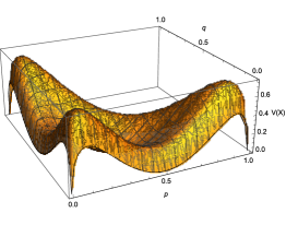
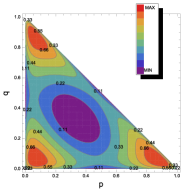
Figure 1: Plots of varentropy (8); left: 3D plot; right: contourplot.

Figure 2: The varentropy corresponding to pdf (9) for $p=q=0.06165$, $0.1$, $0.2$, $0.45$, $0.4$, $0.3$ (from top to bottom for large values of $h$).

The relevance of the entropy in information theory and other disciplines is very well known, whereas the varentropy has attracted less attention. Nevertheless, the latter plays a relevant role in the assessment of the statistical significance of entropy. Specifically, in the discrete case, the entropy (4) represents the expected number of symbols, in natural base, required to code an event produced by a source of information governed by the probability distribution of $X$. In this case, the varentropy (5) measures the variability related to such a coding. In other terms, if two sources of information have the same entropy, than the number of digits required in the average to code two sequences produced by such sources is the same and is proportional to $H(X)$. However, the number of digits required for a single observed sequence in the average is closer to the expected one for the source having the smallest varentropy. Hence, $V(X)$ measures how much the entropy is meaningful in the coding of sequences of symbols generated by $X$.

Example 2.2

Let $Y$ be a Bernoulli random variable having distribution $\mathbb{P}(Y=0)=1-\theta$, $\mathbb{P}(Y=1)=\theta$, with $0\leq\theta\leq 1$. By means of numerical calculations, it is easy to see that for $\theta\approx 0.337009$ one has $H(Y)\approx 0.639032$ and $V(Y)\approx 0.1023$. For the distribution considered in the Example 2.1, if $p=q=0.1$ from (7) and (8), we have $H(X)\approx 0.639032$ and $V(X)\approx 0.691852$, respectively. Hence, the considered random variables have the same entropy, but the varentropy of $X$ is larger. This implies that the coding procedure is much more reliable for sequences generated by $Y$.

2.2 Residual lifetimes

In order to investigate the role of the varentropy in reliability theory, we now recall some relevant notions in this area. Consider a system (such as an item or a living organism) that starts its activity at time 0 and works regularly up to its failure time. Now, we assume that $X$ is a nonnegative absolutely continuous random variable that describes the random lifetime of such a system. Hence, $H(X)$ is a suitable measure of uncertainty of the failure time. However, the use of $H(X)$ is adequate for a brand new system, whereas it is somewhat unrealistic whenever the initial age of the considered system is non-zero. In this case, it is appropriate to recall the residual lifetime

$$X_{t}=[X-t|X>t],\qquad t\in D,$$ (10)

where $D:=\{t\geq 0:\overline{F}(t)>0\}$. Clearly, $X_{t}$ denotes the system lifetime conditioned to the survival of the system at time $t$. The survival function and the pdf of (10), for any $t\in D$, are given respectively by

$$\overline{F}_{t}(x)=\frac{\overline{F}(x+t)}{\overline{F}(t)},\qquad f_{t}(x)=\frac{f(x+t)}{\overline{F}(t)},\qquad x>0.$$ (11)

Hence, recalling (2), the generalization of the entropy to the residual lifetime distributions is given by (see [15], [16], [30])

$$H(X_{t})=\mathbb{E}[IC(X_{t})]=-\int_{t}^{\infty}{\frac{f(x)}{\overline{F}(t)}\log{\frac{f(x)}{\overline{F}(t)}}\,{\rm d}x},\qquad t\in D,$$ (12)

which is named residual entropy, for short. The conventional approach used to characterize the failure distribution of $X$ is either by its (instantaneous) hazard rate function

$$\lambda(t)=\frac{f(t)}{\overline{F}(t)}=\lim_{h\to 0^{+}}\frac{1}{h}\mathbb{P}[X\leq t+h|X>t],\qquad t\in D,$$ (13)

or by its mean residual lifetime function, defined as

$$m(t)=\mathbb{E}(X_{t})=\mathbb{E}[X-t|X>t]=\displaystyle\frac{1}{\overline{F}(t)}\int_{t}^{\infty}{\overline{F}(x)\,{\rm d}x},\qquad t\in D.$$ (14)

For future needs, we recall also the cumulative hazard rate function of $X$,

$$\Lambda(t)=-\log{\overline{F}(t)}=\int_{0}^{t}\lambda(x)\,{\rm d}x,\qquad t\in D,$$ (15)

which plays a relevant role in numerous contexts. Furthermore, we pinpoint the following alternative forms of the residual entropy (12):

$$H(X_{t})=-\Lambda(t)-\frac{1}{\overline{F}(t)}\int_{t}^{\infty}{f(x)}\log{f(x)}\,{\rm d}x,$$ (16a)

$$H(X_{t})=1-\frac{1}{\overline{F}(t)}\int_{t}^{\infty}f(x)\log{\lambda(x)}\,{\rm d}x,$$ (16b)

for $t\in D$. Differentiating relation (16a), one has (see, e.g. Eq. (2.4) of Ebrahimi [15])

$$H^{\prime}(X_{t})=\lambda(t)[H(X_{t})-1+\log{\lambda(t)}].$$ (17)

Moreover, it is known that each of the functions $\overline{F}$, $\lambda$ and $m$ uniquely determines the other two. More specifically, for $t\in D$, we have

$$\overline{F}(t)=\exp\left\{-\int_{0}^{t}{\lambda(x)\,{\rm d}x}\right\}=\frac{m(0)}{m(t)}\exp\left\{-\int_{0}^{t}{\frac{1}{m(x)}\,{\rm d}x}\right\},\qquad\lambda(t)=\frac{m^{\prime}(t)+1}{m(t)}.$$

We recall also that Ebrahimi [15] showed that $H(X_{t})$ uniquely determines $\overline{F}$ under wide assumptions. Useful applications of residual lifetime distributions in actuarial science can be found in Sachlas and Papaioannou [34].

3 Residual varentropy

Recalling that the varentropy of a random lifetime $X$ is defined in (3), we can now extend the notion of varentropy to the residual lifetime considered in (10). Namely, recalling the second of (11), for $t\in D$, we define the varentropy of the residual lifetime distribution (residual varentropy, in short) as

$$\begin{split}V(X_{t})&:={\rm Var}[IC(X_{t})]=\int_{t}^{\infty}{\frac{f(x)}{\overline{F}(t)}\left(\log{\frac{f(x)}{\overline{F}(t)}}\right)^{2}{\rm d}x}-[H(X_{t})]^{2}\\ &=\frac{1}{\overline{F}(t)}\int_{t}^{\infty}{f(x)\left[\log{f(x)}\right]^{2}{\rm d}x}-\left[\Lambda(t)+H(X_{t})\right]^{2},\end{split}$$ (18)

where $\Lambda(t)$ is given in (15), and $H(X_{t})$ is provided in (12) and (16). Making use of Eq. (18) we can show, in Table 1, some examples in which the residual varentropy is constant.

Table 1: Selected distributions with constant varentropy.

Distribution	Pdf	Residual entropy	Residual varentropy
	$f(x)$	$H(X_{t})$	$V(X_{t})$
Uniform	$\displaystyle\frac{1}{\theta}$	$\log{(\theta-t)}$	0
$D=(0,\theta)$
Exponential	$\lambda e^{-\lambda x}$, $\lambda>0$	$1-\log{\lambda}$	1
$D=(0,\infty)$
Triangular	$2(1-x)$	$\displaystyle\frac{1}{2}+\log\frac{1-t}{2}$	$\displaystyle\frac{1}{4}$
$D=(0,1)$

In the following, we determine the conditions for which the residual varentropy is costant. To this aim, we first obtain an expression of its derivative.

Proposition 3.1

For all $t\in D$, the derivative of the residual varentropy is

$$V^{\prime}(X_{t})=\lambda(t)\left\{V(X_{t})-[H(X_{t})+\log\lambda(t)]^{2}\right\}.$$ (19)

• By differentiating both sides of Eq. (18), and recalling (13), we have

  $$V^{\prime}(X_{t})\!\!\!\! = \!\!\!\!\lambda(t)\left\{\frac{1}{\overline{F}(t)}\int_{t}^{\infty}f(x)[\log{f(x)}]^{2}\,{\rm d}x-[\log{f(t)}]^{2}\right\}$$ (20)

  $$\!\!\!\!-2[\Lambda(t)+H(X_{t})][\lambda(t)+H^{\prime}(X_{t})],\qquad t\in D.$$

  Then, making use of Eqs. (17) and (18), from (20) we get

  $$V^{\prime}(X_{t})\!\!\!\! = \!\!\!\!\lambda(t)\left\{V(X_{t})+[\Lambda(t)+H(X_{t})]^{2}-[\log{f(t)}]^{2}\right.$$

  $$\!\!\!\!\left.-2[\Lambda(t)+H(X_{t})][H(X_{t})+\log\lambda(t)]\right\},\qquad t\in D.$$

  Hence, due to (15), after some calculations, we obtain Eq. (19).

As a consequence of Proposition 3.1, we can now provide some useful results involving the residual varentropy, the residual entropy, the hazard rate, and the varentropy of a lifetime $X$.

Theorem 3.1

Let $X$ have a pdf such that $f(t)>0$ for all $t\in(0,r)$, with $r\in(0,\infty]$.
(i)  If the residual varentropy $V(X_{t})$ is constant, say

$$V(X_{t})=v\geq 0,\qquad\forall t\in[0,r),$$ (21)

then the following relation holds:

$$|H(X_{t})+\log{\lambda(t)}|=\sqrt{v},\qquad\forall t\in(0,r).$$ (22)

(ii)  Let $c\in\mathbb{R}$; if

$$H(X_{t})+\log{\lambda(t)}=c,\qquad\forall t\in(0,r),$$ (23)

then

$$V(X_{t})=c^{2}+\frac{V(X)-c^{2}}{\overline{F}(t)},\qquad\forall t\in[0,r).$$ (24)

• Since $f(t)>0$ for all $t\in(0,r)$, the assumption (21) immediately gives (22), due to (19). Moreover, if condition (23) holds, then Eq. (19) becomes

  $$V^{\prime}(X_{t})=\lambda(t)\left\{V(X_{t})-c^{2}\right\},\qquad t\in(0,r),$$

  with initial condition $V(X_{t})|_{t=0}=V(X)$. Finally, it is not hard to see that the solution of such problem yields Eq.  (24).

Let us now recall the notion of generalized hazard (or failure) rate of $X$ expressed by (see Schweizer and Szech [36])

$$\lambda_{\alpha}(t)=\frac{f(t)}{[\overline{F}(t)]^{1+\alpha}},\qquad t\in D,$$ (25)

for $\alpha\in\mathbb{R}$. Clearly, recalling (13), one has $\lambda_{0}(t)=\lambda(t)$ for all $t$. Other parameterizations of $\lambda_{\alpha}(t)$ have been treated in Bieniek and Szpak [5] as a special case of the generalized failure rate defined by Barlow and van Zwet [4]. Further forms of generalized hazard rates have been considered in the past. For instance, Lariviere and Porteus [24], and Maoui et al. [29] considered $t\,\lambda(t)$ as generalized hazard rate. Moreover, a different version has been treated in Li and Tewari [25].

We are now able to provide necessary and sufficient conditions in terms of the residual entropy (cf. point (ii) of Theorem 3.1), such that the generalized hazard rate of $X$ is constant. Recall that $H(X)$ denotes the entropy given in (2).

Theorem 3.2

Let $X$ possess a pdf such that $f(t)>0$ for all $t\in(0,r)$, with $r\in(0,\infty]$. The generalized hazard rate of $X$ is constant, such that

$$\lambda_{c-1}(t)=e^{c-H(X)},\qquad t\in[0,r),$$ (26)

if and only if Eq. (23) is fulfilled for a given $c\in\mathbb{R}$.

• Assume that the Eq. (26) is fulfilled. Making use of (13) and (16a), we have

  $$H(X_{t})+\log{\lambda(t)}=\log{f(t)}+\frac{1}{\overline{F}(t)}\left\{H(X)+\int_{0}^{t}f(x)\log{f(x)}\,\mathrm{d}x\right\}.$$ (27)

  From the assumption (26) it is not hard to see that

  $$\int_{0}^{t}f(x)\log{f(x)}\,\mathrm{d}x=-F(t)\,H(X)-c\,\overline{F}(t)\log\overline{F}(t).$$

  Hence, due to Eqs. (26) and (27), we have

  $$H(X_{t})+\log{\lambda(t)}=H(X)+\log\frac{f(t)}{[\overline{F}(t)]^{c}}=c,$$

  so that (23) holds. Now, let us prove that (23) implies the validity of Eq. (26). In fact, rearranging Eq. (17), we have

  $$H(X_{t})+\log\lambda(t)=\frac{H^{\prime}(X_{t})}{\lambda(t)}+1,$$

  so that, due to Eq. (23), one has

  $$H^{\prime}(X_{t})=(c-1)\lambda(t),\qquad t\in(0,r).$$

  By integration over $[0,t]$, and recalling (15), one obtains

  $$H(X_{t})-H(X)=(c-1)\Lambda(t),\qquad t\in[0,r).$$

  Comparing the latter identity with Eq. (23) and in virtue of (15), after some algebraic calculations, we get

  $$\log\frac{f(t)}{[\overline{F}(t)]^{c}}=c-H(X),$$

  which gives immediately relation (26) by virtue of (25).

Remark 3.1

(i) It is worth pointing out that, due to Theorem 3.1 of Asadi and Ebrahimi [3], the condition expressed in Eq. (23) is fulfilled if and only if $X$ has a generalized Pareto distribution, with survival function

$$\overline{F}(t)=\left(\frac{b}{at+b}\right)^{\frac{1}{a}+1},\qquad t\geq 0,$$ (28)

for $a>-1$ and $b>0$. The generalized Pareto distribution is a flexible statistical model which is employed in several research areas, such as statistical physics, econophysics and social sciences, since its distribution possesses a tail of general form. Specifically, it includes the exponential distribution ($a\to 0$), the Pareto distribution ($a>0$, with heavy tail), and the power distribution ($-1<a<0$, with bounded support). An intuitive reason leading to the above result is due to the property that the generalized Pareto distribution is the only family of distributions whose mean residual function (14) is linear (see Hall and Wellner [20]). Indeed, for the survival function (28) we have $m(t)=at+b$, with hazard rate function $\lambda(t)=\frac{1+a}{at+b}$. For a recent characterization of this distribution in the context of shape functionals, see Arriaza et al. [2].
(ii) A special case arises from (28) in the limit as $a\to\infty$ and $b\to\infty$, with $\frac{a}{b}\to\lambda>0$, by which the pdf and the survival function of $X$ are given, respectively, by

$$f(t)=\frac{\lambda}{(1+\lambda t)^{2}},\qquad\overline{F}(t)=\frac{1}{1+\lambda t},\qquad t\in[0,\infty).$$

In this case, $X$ has a modified Pareto distribution that describes the first arrival time in a Geometric counting process with parameter $\lambda>0$ (cf. Section 2.2 of [14], for instance). From Eq. (25), it immediately follows that the generalized hazard rate of $X$ is a constant for $\alpha=1$, i.e. $\lambda_{1}(t)\equiv\lambda$. As a consequence, Eq. (26) is fulfilled for $c=2$ and $H(X)=2-\log\lambda$. From Theorems 3.1 and 3.2, we thus obtain the (increasing) residual entropy,

$$H(X_{t})=2-\log\frac{\lambda}{1+\lambda t},\qquad t\geq 0,$$

and the corresponding constant residual varentropy, $V(X_{t})=4$. It is worth pointing out that in this special case, the mean residual lifetime is infinite. Hence, for such a stochastic model the residual entropy and the residual varentropy provide useful information even if the mean residual lifetime is not finite.

The following example is concerning a family of distributions for which the residual varentropy exhibits different behaviors.

Example 3.1

Let $X_{\lambda,k}$ have Weibull distribution, with pdf

$$f_{\lambda,k}(x)=\frac{k}{\lambda}\left(\frac{x}{\lambda}\right)^{k-1}e^{-({x}/{\lambda})^{k}},\qquad x>0,$$ (29)

where $k>0$ is the shape parameter and $\lambda>0$ is the scale parameter. Recall that this family of distributions includes special cases of interest, such as the exponential distribution (for $k=1$) and the Rayleigh distribution (for $k=2$). A characterization of the Weibull distribution in terms of a Gini-type index of interest in reliability theory is provided in Theorem 1 of [33]. The expression of the residual varentropy is omitted being quite cumbersome. The behavior of the pdf (29) and of the corresponding residual varentropy is visualized in Fig. 3 for some choices of the shape parameter. It can be seen that the residual varentropy is decreasing, constant, increasing, non monotonic for $k=0.5$, $1$, $1.5$, $3.5$ respectively.

   

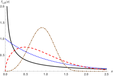
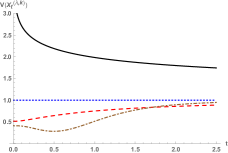
Figure 3: (left) Weibull pdf, given in (29), and (right) residual varentropy for $\lambda=1$ and various choices of $k$ (as indicated in the label).

Let us now analyze the effect of linear transformations to the residual varentropy. We recall that if

$$Y=aX+b,\qquad a>0,\quad b\geq 0,$$ (30)

then the residual entropy of $X$ and $Y$ are related by (see Eq. (2.6) of Ebrahimi and Pellerey [16])

$$H(Y_{t})=H\left(X_{\frac{t-b}{a}}\right)+\log a,\qquad\forall\ t.$$ (31)

Proposition 3.2

Let $X$ and $Y$ be related by (30). Hence, for their residual varentropies, we have:

$$V(Y_{t})=V\left(X_{\frac{t-b}{a}}\right)\qquad\forall\ t.$$ (32)

• Clearly, from (30) we have that the cdfs and the pdfs of $Y$ and $X$ are related by $F_{Y}(x)=F_{X}\left(\frac{x-b}{a}\right)$ and $f_{Y}(x)=\frac{1}{a}\ f_{X}\left(\frac{x-b}{a}\right)$. Hence, recalling (18) and (31), it is not hard to see that

  $$V(Y_{t})=\int_{\frac{t-b}{a}}^{\infty}{\frac{f_{X}(x)}{\overline{F}_{X}(\frac{t-b}{a})}\left[\log{\frac{f_{X}(x)}{\overline{F}_{X}(\frac{t-b}{a})}}-\log{a}\right]^{2}\mathrm{d}x}-\left[H\left(X_{\frac{t-b}{a}}\right)+\log{a}\right]^{2}.$$

  The thesis (32) thus follows after some calculations.

3.1 Bounds

We conclude this section by discussing some bounds to the residual varentropy.

First, we provide a lower bound for $V(X_{t})$. It will be expressed in terms of the “variance residual life function”, defined as the variance of (10), that is,

$$\sigma^{2}(t)={\rm Var}(X_{t})={\rm Var}[X-t|X>t]=\frac{2}{\overline{F}(t)}\int_{t}^{\infty}{\rm d}x\int_{x}^{\infty}\overline{F}(y)\,{\rm d}y-[m(t)]^{2},$$ (33)

with $m(t)$ defined in (14). For instance, see Gupta [19] for characterization results and properties of $\sigma^{2}(t)$.

Theorem 3.3

Let $X_{t}$ be a residual lifetime as defined in (10), and assume that the corresponding mean residual lifetime $m(t)$ and variance residual lifetime $\sigma^{2}(t)$ are finite (cf. (14) and (33), respectively). Then, for all $t\in D$,

$$V(X_{t})\geq\sigma^{2}(t)\,(\mathbb{E}[w_{t}^{\prime}(X_{t})])^{2}$$ (34)

where the function $w_{t}(x)$ is defined by

$$\sigma^{2}(t)\,w_{t}(x)\,f_{t}(x)=\int_{0}^{x}{[m(t)-z]\,f_{t}(z)\,{\rm d}z},\qquad x>0,$$

with $f_{t}(x)$ given in the second of (11).

• We recall that if $X$ is an absolutely continuous random variable with pdf $f(x)$, mean $\mu$ and variance $\sigma^{2}$, then (cf. Cacoullos and Papathanasiou [7])

  $${\rm Var}[g(X)]\geq\sigma^{2}(\mathbb{E}[w(X)g^{\prime}(X)])^{2},$$ (35)

  where $w(x)$ is defined by $\sigma^{2}w(x)f(x)=\int_{0}^{x}(\mu-z)f(z)\,{\rm d}z$. Hence, by taking $X_{t}$ as reference, with $g(x)=-\log f(x)$ and integrating by parts, similarly as Eq. (3.9) of Goodarzi et al. [18], we obtain (34).

Note that the equality in (35) holds if and only if $X$ is exponentially distributed.

Hereafter, we determine suitable upper bounds to the residual varentropy, thus providing conditions on its finiteness. First, we recall that $X$ is said to be ILR (increasing in likelihood ratio) if its pdf $f(x)$ is such that $\log f(x)$ is a concave function on $(0,\infty)$; equivalently, we say that $X$ has a log-concave pdf.

Theorem 3.4

Given a random lifetime $X$ with log-concave pdf $f(x)$, then

$$V(X_{t})\leq 1,\qquad\hbox{for all $t\in D$}.$$

• We note that if $f(x)$ is log-concave, then also $f_{t}(x)$ is log-concave due to (11). Hence, the proof is a direct consequence of Theorem 2.3 of Fradelizi et al. [17], which states that the varentropy of a random lifetime with log-concave pdf is not greater than 1.

The following bound is expressed in terms of the weighted residual entropy of $X$, which is a weighted version of the residual entropy (12) and is given by (see Di Crescenzo and Longobardi [12] for details)

$$H^{w}(X_{t})\!\!\!\! = \!\!\!\!-\int_{t}^{\infty}x\,{\frac{f(x)}{\overline{F}(t)}\log{\frac{f(x)}{\overline{F}(t)}}\,{\rm d}x}$$ (36)

$$= \!\!\!\!-\frac{1}{\overline{F}(t)}\int_{t}^{\infty}x\,f(x)\log{f(x)}{\rm d}x-\frac{\Lambda(t)}{\overline{F}(t)}\int_{t}^{\infty}x\,f(x){\rm d}x,\qquad t\in D.$$

Furthermore, it is based on the so-called vitality function of $X$, i.e.

$$\delta(t):=\mathbb{E}[X|X>t]=m(t)+t,\qquad t\in D.$$ (37)

Namely, since $X$ denotes the random lifetime of a system, $\delta(t)$ can be interpreted as the average life span of a system whose age exceeds $t$.

Theorem 3.5

If $X$ is a random lifetime such that its pdf satisfies

$$e^{-\alpha x-\beta}\leq f(x)\leq 1\qquad\forall x\geq 0,$$ (38)

with $\alpha>0$ and $\beta\geq 0$, then for all $t\geq 0$

$$V(X_{t})\leq\alpha[\Lambda(t)\delta(t)+H^{w}(X_{t})]+\beta[\Lambda(t)+H(X_{t})]-[\Lambda(t)+H(X_{t})]^{2}.$$ (39)

• From Eq. (18), due to (38) one has

  $$V(X_{t})\leq-\frac{1}{\overline{F}(t)}\int_{t}^{\infty}(\alpha x+\beta)f(x)\log{f(x)}{\rm d}x-\left[\Lambda(t)+H(X_{t})\right]^{2},\qquad t\geq 0.$$ (40)

  We note that Eqs. (14) and (37) give

  $$\int_{t}^{\infty}x\,f(x){\rm d}x=\overline{F}(t)\delta(t),\qquad t\geq 0.$$

  Hence, recalling (15) and (37), Eq. (36) implies:

  $$\int_{t}^{\infty}x\,f(x)\log{f(x)}{\rm d}x=-\overline{F}(t)[\Lambda(t)\delta(t)+H^{w}(X_{t})],\qquad t\geq 0.$$ (41)

  Moreover, from (16a), we have

  $$\int_{t}^{\infty}f(x)\log{f(x)}{\rm d}x=-\overline{F}(t)[\Lambda(t)+H(X_{t})],\qquad t\geq 0.$$ (42)

  Finally, substituting (41) and (42) in (40), we immediately obtain the inequality (39).

4 Some applications

In this section, we consider some applications of the residual varentropy. We first deal with the proportional hazard rates model, which in turn can be employed to the reliability analysis of series systems. A further case of interest is concerning the first-passage-time problem of an Ornstein-Uhlenbeck jump-diffusion process which arises as a limit of the continuous-time Ehrenfest model.

4.1 Proportional hazards model

Consider a family of absolutely continuous nonnegative random variables $\{X^{(a)};a>0\}$, where the survival function and the pdf of $X^{(a)}$ are expressed, respectively, as

$$\overline{F}^{(a)}(t)=\mathbb{P}[X^{(a)}>t]=[\overline{F}(t)]^{a},\quad f^{(a)}(t)=a[\overline{F}(t)]^{a-1}f(t),\qquad t>0,$$ (43)

with $\overline{F}(t)$ a suitable baseline survival function and $f(t)=-\frac{\mathrm{d}}{\mathrm{d}t}\overline{F}(t)$ the associated pdf. This model is known as the proportional hazards model, see Cox [9], since the hazard rate function of $X^{(a)}$ is proportional to the hazard rate corresponding to the baseline survival function. For instance, see Parsa et al. [33] for a recent characterization of the proportional hazards model in terms of the Gini-type index.

Let us now address the problem of evaluating the residual varentropy for the model (43) when $X^{(a)}$ is a random lifetime. First, noting that the cumulative hazard rate function is given by

$$\Lambda^{(a)}(t)=-\log{\overline{F}^{(a)}(t)}=a\,\Lambda(t),\qquad t>0,$$ (44)

from (16a), it is not hard to see that the residual entropy of $X^{(a)}$ is expressed as

$$H(X_{t}^{(a)})\!\!\!\! = \!\!\!\!-\Lambda^{(a)}(t)-\frac{1}{[\overline{F}(t)]^{a}}\int_{t}^{\infty}{f^{(a)}(x)\log{f^{(a)}(x)}}\,{\rm d}x$$ (45)

$$= \!\!\!\!-a\,\Lambda(t)-\frac{1}{[\overline{F}(t)]^{a}}\int_{0}^{[\overline{F}(t)]^{a}}\ell(y;a)\,{\rm d}y,\qquad t>0,$$

with $y=[\overline{F}(x)]^{a}$, and where

$$\ell(y;a):=\log{\left\{a\,y^{1-1/a}\,f[\overline{F}^{-1}(y^{1/a})]\right\}},\qquad 0<y<1.$$ (46)

Hence, recalling (18), from (44) and (45) after some calculations, we obtain the residual varentropy of $X^{(a)}$, for $t>0$:

$$V(X_{t}^{(a)})\!\!\!\! = \!\!\!\!\frac{\int_{t}^{\infty}{f^{(a)}(x)[\log{f^{(a)}(x)}}]^{2}\,{\rm d}x}{[\overline{F}(t)]^{a}}-\left[\frac{\int_{t}^{\infty}{f^{(a)}(x)\log{f^{(a)}(x)}}\,{\rm d}x}{[\overline{F}(t)]^{a}}\right]^{2}$$ (47)

$$= \!\!\!\!\frac{1}{[\overline{F}(t)]^{a}}\int_{0}^{[\overline{F}(t)]^{a}}[\ell(y;a)]^{2}\mathrm{d}y-\left\{\frac{1}{[\overline{F}(t)]^{a}}\int_{0}^{[\overline{F}(t)]^{a}}\ell(y;a)\,\mathrm{d}y\right\}^{2}.\quad$$

Making use of Eqs. (13) and (15), one has $f(x)=\lambda(x)e^{-\Lambda(x)}$, so that the function introduced in (46) can be rewritten also as follows:

$$\ell(y;a)=\log{\Big{\{}ay\lambda\Big{(}\Lambda^{-1}\Big{(}-\frac{1}{a}\log{y}\Big{)}\Big{)}\Big{\}}}.$$

An application can be immediately given to series systems.

Example 4.1

Consider a system composed of $n$ units in series and characterized by i.i.d. random lifetimes $X_{1},\ldots,X_{n}$. Let the survival function of each unit be denoted with $\overline{F}(t)=\mathbb{P}(X_{i}>t)$. Since the system lifetime is given by $X^{(n)}=\min\{X_{1},\ldots,X_{n}\}$, the model of series system satisfies the proportional hazards model specified in (43), for $a=n\in\mathbb{N}$.

For an illustrative example, we assume that the random lifetimes $X_{i}$ have generalized exponential distribution with survival function $\overline{F}(t)=1-(1-e^{-\lambda t})^{b}$, $t\geq 0$, for $b>0$. (We recall that this distribution plays a role in the construction of probabilistic models for damped random motions with finite velocities [13]). From (46), thus we have

$$\ell(y;a)=\log\left\{ab\lambda y^{1-\frac{1}{a}}(1-y)^{1-\frac{1}{b}}\big{[}1-(1-y)^{\frac{1}{b}}\big{]}\right\},\qquad 0<y<1.$$

From Eq. (47), we come to the residual varentropy of the system lifetime $X^{(n)}$. The expression of $V(X_{t}^{(a)})$ cannot be obtained in closed form, but it can be evaluated via numerical computations. Figure 4 shows some plots of the residual varentropy for some choices of $a=n$. It is clear that the varentropy increases when the number of units grows, and generally when $t$ becomes larger.

 

 

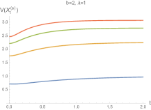
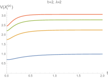
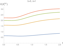
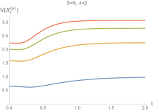
Figure 4: The residual varentropy of $X_{t}^{(a)}$ for the series system of Example 4.1, for $a=n=1,2,3,4$ (from bottom to top) and for $b$ and $\lambda$ as indicated.

Example 4.2

Under the proportional hazards model, Eq. (47) can be used to construct time-varying reference sets for the information content of the residual lifetime (10). Specifically, we determine intervals of the form

$$H(X_{t}^{(a)})\pm k\sqrt{V(X_{t}^{(a)})}=\mathbb{E}[IC(X_{t}^{(a)})]\pm k\sqrt{{\rm Var}[IC(X_{t}^{(a)})]},\qquad k=2,3$$ (48)

for suitable baseline distributions (Weibull, gamma and lognormal). Since closed forms are not available, we illustrate such results with some graphics given in Figure 5. For comparison purposes, the relevant parameters are chosen in order that the baseline distributions have unity means.

 

 

 

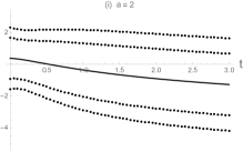
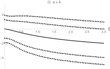
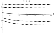
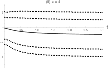
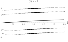
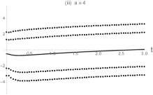
Figure 5: Residual entropy $H(X_{t}^{(a)})$ (full) and extremes of the intervals (48) (dotted) with $a=2$ (left) and $a=4$ (right), for the following baseline pdfs:
(i)  (Weibull) $f(t)=\frac{k}{\lambda}\left(\frac{t}{\lambda}\right)^{k-1}\exp\{-\left(\frac{t}{\lambda}\right)^{k}\}$, $t>0$, for $k=2$, $\lambda=\frac{2}{\pi}$;
(ii)  (gamma) $f(t)=\frac{1}{\theta}\left(\frac{t}{\theta}\right)^{r-1}\exp\left\{-\frac{t}{\theta}\right\}\frac{1}{\Gamma(r)}$, $t>0$, for $r=2$, $\theta=\frac{1}{2}$;
(iii)  (lognormal) $f(t)=\frac{1}{\sqrt{2\pi}\sigma t}\exp\left\{-\frac{(\log t-\mu)^{2}}{2\sigma^{2}}\right\}$, $t>0$, for $\mu=-\frac{1}{2}$, $\sigma=1$.

4.2 First-passage times of an Ornstein-Uhlenbeck jump-diffusion process

The continuous-time Ehrenfest model describes a simple diffusion process as a suitable Markov chain, where molecules of a gas diffuse at random in a container divided into two equal parts by a permeable membrane. Recently, Dharmaraja et al. [11] proposed an extension of such stochastic system that includes the occurrence of stochastic resets, also named ‘catastrophes’, i.e. instantaneous transitions to the state zero at constant rate $\xi>0$. A jump-diffusion approximation was considered under a suitable scaling procedure. Specifically, the resulting jump-diffusion process, say $\{X(t),t\geq 0\}$, consists in a mean-reverting time-homogenous Ornstein-Uhlenbeck process with catastrophes (occurring with rate $\xi$), having state-space $\mathbb{R}$, with drift and infinitesimal variance given by

$$A_{1}(x)=-\alpha x,\qquad A_{2}(x)=\alpha\nu\qquad(\alpha>0,\nu>0).$$

In this case, denoting by $f(t)$ the first-passage-time (FPT) pdf of $X(t)$ through 0, with $X(0)=y\neq 0$, we have (cf. Eq. (49) of [11])

$$f(t)=e^{-\xi t}\,\widetilde{f}(t)+\xi\,e^{-\xi t}{\rm Erf}\left(|y|e^{-\alpha t}\,[\nu(1-e^{-2\alpha t})]^{-1/2}\right),\qquad t>0,$$ (49)

with $f(0)=\xi$, where ${\rm Erf}(\cdot)$ is the error function, and where (cf. Eq. (38) of [11])

$$\widetilde{f}(t)={2\alpha|y|e^{-\alpha t}\over\sqrt{\pi\nu}\left(1-e^{-2\alpha t}\right)^{3/2}}\exp\biggl{\{}-\,{y^{2}e^{-2\alpha t}\over\nu(1-e^{-2\alpha t})}\biggr{\}},\qquad t>0,$$

with $\widetilde{f}(0)=0$, is the FPT pdf of the corresponding diffusion process in absence of catastrophes. We recall that the FPT pdf (49) deserves interest in the realm of stochastic processes with stochastic reset (see, for instance, Kusmierz et al. [23] and Pal [32]). To analyze the relevant information content, Figures 6 and 7 show some instances of the residual entropy related to pdf (49), whereas the corresponding residual varentropy is provided in Figures 8 and 9. It is shown that the residual entropy is decreasing in $\xi$ and in $\nu$; moreover, it tends to a constant when $t$ grows, such limit being decreasing in $\xi$ and constant in $\nu$. The residual varentropy exhibits a different behavior, since it is decreasing in $\xi$ and is increasing in $\nu$ for sufficiently large values of $t$. Moreover, it tends to an identical limit when $t$ grows. This latter property is confirmed by extensive computations performed for various choices of the parameters.

 

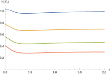
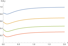
Figure 6: Residual entropy for the FPT pdf (49), when $y=1$, $\alpha=1$, $\nu=1$ (left), $\nu=2$ (right), and $\xi=0$, $0.35$, $0.7$, $1$ (from top to bottom).

 

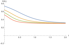
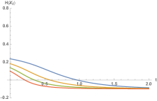
Figure 7: Same as Figure 6, for $\xi=1$ (left), $\xi=2$ (right), and $\nu=0.15$, $0.3$, $0.45$, $0.6$ (from top to bottom).

 

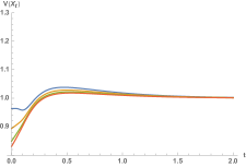
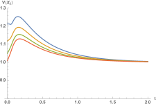
Figure 8: Residual varentropy for the same cases of Figure 6, with $\xi=0$, $0.35$, $0.7$, $1$ (from top to bottom).

 

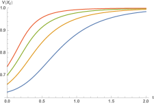
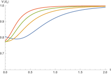
Figure 9: Residual varentropy for the same cases of Figure 7, with $\nu=0.15$, $0.3$, $0.45$, $0.6$ (from bottom to top).

5 Conclusions

The differential entropy (2) is largely used in information theory and other related areas, being the analogue of the Shannon entropy for a continuous random variable. It constitutes the expected value of the information content (1), whereas its variance is given by the varentropy (3). The latter is useful to assess the effectiveness of the differential entropy as a measure of the information content of a random system.

Motivated by possible application in reliability theory and survival analysis, in this paper we investigated the residual varentropy, that is the varentropy of the residual lifetime distribution. Together with the residual entropy, this measure allows to analyze the dynamical information content of time-varying systems conditional on being active at current time. We discussed various properties, with connections to the generalized hazard rate, the effect of linear transformations, and a suitable lower bound that involves the variance residual life function. We also addressed the use of the residual varentropy in connection with classical distributions and within some applications concerning the proportional hazards model and the first-passage time problem of an Ornstein-Uhlenbeck jump-diffusion process with catastrophes.

Future developments will be oriented to applications of the varentropy to other stochastic models of interest (such as order statistics, spacings, record values, inaccuracy measures based on the relevation transform and its reversed version) and to construct an empirical version of the residual varentropy in order to come to suitable estimates.

Acknowledgements

The authors are members of the research group GNCS of INdAM. (Istituto Nazionale di Alta Matematica). This research is partially supported by MIUR - PRIN 2017, project ‘Stochastic Models for Complex Systems’, no. 2017JFFHSH.

References

- [1] Arikan, E. (2016). Varentropy decreases under polar transform. IEEE Transactions on Information Theory 62:3390-3400.
- [2] Arriaza, A., Di Crescenzo, A., Sordo, M.A., & Suárez-Llorens, A. (2019). Shape measures based on the convex transform order. Metrika 82:99-124.
- [3] Asadi, M., & Ebrahimi, N. (2000). Residual entropy and its characterizations in terms of hazard function and mean residual life function. Statistics and Probability Letters 49:263-269.
- [4] Barlow, R.E., & van Zwet, W. (1970). Asymptotic properties of isotonic estimators for the generalized failure rate function. I. Strong consistency. In M.L. Puri (ed.), Nonparametric techniques in statistical inference. London, Cambridge University Press, pp. 159-176.
- [5] Bieniek, M., & Szpak, M. (2018). Sharp bounds for the mean of the total time on test for distributions with increasing generalized failure rate. Statistics 52:818-828.
- [6] Bobkov, S., & Madiman, M. (2011). Concentration of the information in data with log-concave distributions. Annals of Probability 39:1528-1543.
- [7] Cacoullos, T., & Papathanasiou, V. (1989). Characterizations of distributions by variance bounds. Statistics and Probability Letters 7:351-356.
- [8] Cover, T.M., & Thomas, J.A. (1991). Elements of Information Theory. New York: J. Wiley & Sons.
- [9] Cox, D.R. (1959). The analysis of exponentially distributed lifetimes with two types of failure. Journal of the Royal Statistical Society. Series B 21:411-421.
- [10] Cufaro Petroni, N. (2014). Entropy and its discontents: A note on definitions. Entropy 16:4044-4059.
- [11] Dharmaraja, S., Di Crescenzo, A., Giorno, V., & Nobile, A.G. (2015). A continuous-time Ehrenfest model with catastrophes and its jump-diffusion approximation. Journal of Statistical Physics 161:326-345.
- [12] Di Crescenzo, A., & Longobardi, M. (2006). On weighted residual and past entropies. Scientiae Mathematicae Japonicae 64:255-266.
- [13] Di Crescenzo, A., & Martinucci, B. (2010). A damped telegraph random process with logistic stationary distribution. Journal of Applied Probability 47:84-96.
- [14] Di Crescenzo, A., & Pellerey, F. (2019). Some results and applications of geometric counting processes. Methodology and Computing in Applied Probability 21:203-233.
- [15] Ebrahimi, N. (1996). How to measure uncertainty in the residual life time distribution. Sankhyā. The Indian Journal of Statistics. Series A 58:48-56.
- [16] Ebrahimi, N., & Pellerey, F. (1995). New partial ordering of survival functions based on the notion of uncertainty, Journal of Applied Probability 32:202-211.
- [17] Fradelizi, M., Madiman, M., & Wang, L. (2016). Optimal concentration of information content for log-concave densities. In C. Houdré, D. Mason, P. Reynaud-Bouret & J. Rosiński (eds.), High Dimensional Probability VII. Progress in Probability, vol. 71, Cham, Springer, pp. 45-60.
- [18] Goodarzi, F., Amini, M., & Borzadaran, G.R.M. (2017). Characterizations of continous distributions through inequalities involving the expected values of selected functions. Applications of Mathematics 62:493-507.
- [19] Gupta, R.C. (2006). Variance residual life function in reliability studies, Metron 64:343-355.
- [20] Hall, W.J., & Wellner, J.A. (1981). Mean residual life. In M. Csörgö, D.A. Dawson, J.N.K. Rao & A.K.Md.E. Saleh (eds.), Statistics and Related Topics, North-Holland, pp. 169-184.
- [21] Kontoyiannis, I., & Verdú, S. (2013). Optimal lossless compression: source varentropy and dispersion. IEEE International Symposium on Information Theory, Istanbul, pp. 1739-1743.
- [22] Kontoyiannis, I. & Verdú, S. (2014). Optimal lossless data compression: non-asymptotics and asymptotics. IEEE Transactions on Information Theory 60:777-795.
- [23] Kusmierz, L., Majumdar, S.N., Sabhapandit, S., & Schehr, G. (2014). First order transition for the optimal search time of Lévy flights with resetting. Physical Review Letters 113:220602.
- [24] Lariviere, M.A., & Porteus, E.L. (2001). Selling to the newsvendor: an analysis of price-only contracts. Manufacturing & Service Operations Management 3:293-305.
- [25] Li, Z., & Tewari, A. (2018). Beyond the hazard rate: more perturbation algorithms for adversarial multi-armed bandits. Journal of Machine Learning Research18:1-24.
- [26] Li, J., Fradelizi, M., & Madiman, M. (2016). Information concentration for convex measures. IEEE International Symposium on Information Theory, Barcelona, 1128-1132.
- [27] Madiman, M., & Barron, A. (2007). Generalized entropy power inequalities and monotonicity properties of information. IEEE Transactions on Information Theory 53:2317-2329.
- [28] Madiman, M., & Wang, L. (2014). An optimal varentropy bound for log-concave distributions. International Conference on Signal Processing and Communications (SPCOM), Bangalore , 1 p. doi: 10.1109/SPCOM.2014.6983953
- [29] Maoui, I., Ayhan, H., & Foley, R. (2007). Congestion-dependent pricing in a stochastic service system. Advances in Applied Probability 39:898-921.
- [30] Muliere, P., Parmigiani, G., & Polson, N.G. (1993). A note on the residual entropy function. Probability in the Engineering and Informational Sciences 7:413-420.
- [31] Nanda, A.K., & Chowdhury, S. (2019). Shannon’s entropy and its generalizations towards statistics. reliability and information science during 1948-2018. 18 pp. arXiv:1901.09779v1
- [32] Pal, A. (2015). Diffusion in a potential landscape with stochastic resetting. Physical Review E 91:012113.
- [33] Parsa, M., Di Crescenzo, A., & Jabbari, H. (2018). Analysis of reliability systems via Gini-type index. European Journal of Operational Research 264:340-353.
- [34] Sachlas, A., & Papaioannou, T. (2014). Residual and past entropy in actuarial science and survival models. Methodology and Computing in Applied Probability 16:79-99.
- [35] Schroeder, M.J. (2004). An alternative to entropy in the measurement of information. Entropy 6:388-412.
- [36] Schweizer, N., & Szech, N. (2015). A quantitative version of Myerson regularity. Working Paper Series in Economics 76, Karlsruhe Institute of Technology (KIT), Department of Economics and Business Engineering, 18 pp.
- [37] Shannon, C.E. (1948). A mathematical theory of communication. Bell System Technical Journal 27:379-423,623-656.
- [38] Verdú, S., & Kontoyiannis, I. (2012) Lossless data compression rate: asymptotics and non-asymptotics. In 46th Annual Conference on Information Sciences and Systems (CISS), Princeton, NJ, 6 pp. doi: 10.1109/CISS.2012.6310950