A Review of Reduced-Order Models for Microgrids: Simplifications vs Accuracy

Abstract

Inverter-based microgrids are an important technology for sustainable electrical power systems and typically use droop-controlled grid-forming inverters to interface distributed energy resources to the network and control the voltage and frequency. Ensuring stability of such microgrids is a key issue, which requires the use of appropriate models for analysis and control system design. Full-order detailed models can be more difficult to analyze and increase computational complexity, hence a number of reduced-order models have been proposed in the literature which present various trade-offs between accuracy and complexity. However, the se simplifications present the risk of failing to adequately capture important dynamics of the microgrid. Therefore, there is a need for a comprehensive review and assessment of their relative quality, which is something that has not been systematically carried out thus far in the literature and we aim to address in this paper. In particular, we review various inverter-based microgrid reduced-order models and investigate the accuracy of their predictions for stability via a comparison with a corresponding detailed average model. Our study shows that the simplifications reduced order models rely upon can affect their accuracy in various regimes of the line R/X ratios, and that inappropriate model choices can result in substantially inaccurate stability results. Finally, we present recommendations on the use of reduced order models for the stability analysis of microgrids.

I INTRODUCTION

Increasing environmental concerns, advancement in renewable energy technologies and the continuous rise in the global energy demand bring about the exploration of renewable energy sources. Most of these sources are small-scale distributed energy generation (DG) units and will form microgrids, which are the interconnection of DG units, loads, and energy storage systems into a controllable system. Microgrids can be operated in grid-connected or autonomous mode, and autonomous microgrids are an especially effective solution for remote areas where the main power grid is not accessible [1, 2, 3]. Most renewable energy sources cannot be effectively utilised without power conditioners [4, 5, 6, 7, 8], and power converters are becoming increasingly common as interfaces that provide the power conditioning capability. They now appear in higher power ratings and are therefore an integral part of microgrid dynamics.

There are new challenges associated with microgrids. With the increasing proportion of DG units, especially in the autonomous mode of operation, there is a need for individual inverters to achieve power sharing. Power sharing is the ability of microgrid inverters to optimally allocate their power outputs to meet the load demand in the network, while achieving a desired steady-state (characterised by the steady-state frequency and voltage). It is desirable to achieve this via the local measurements (voltages and currents) provided to the inverters’ local controllers. The droop control policy offers this feature and is widely used [9, 10, 11, 12, 13, 14, 15, 16, 17, 18]. Local measurements are used to adjust the inverters’ frequency and voltage setpoints based on the corresponding demand of active and reactive power respectively. The droop gains are chosen to specify the active and reactive power sharing ratio among inverters, however this choice strongly affects the dynamics and stability of microgrids [10, 11, 12, 19, 20, 21]. The nonlinearity of this control scheme increases the complexity of the closed loop microgrid dynamics, and severe stability issues have been noted in previous studies [22, 23, 24]. There is hence a need for stability issues to be accurately assessed via appropriate mathematical models.

Accurate mathematical representation of inverters is fundamental for the modelling and stability assessment of inverter-based microgrids. Inverters are usually controlled via pulse-width modulation (PWM) schemes [25, 26, 27, 28]. The discontinuity of trajectories in this scheme increases the complexity of inverter dynamics and a common approach to address this is the use of the averaging theory, which allows inverters to be represented as continuous time systems [29, 30, 31, 10, 32]. Such models are used either for frequency domain analysis [31, 33, 34, 35, 36, 37], or analysis in the time domain [10, 22, 38]. The latter allows for both small-signal and large signal models to be formulated, and provides additional insight into dynamic interactions [10].

Models used to describe the behaviour of inverter-based microgrids consist of the inverter and power lines dynamics, and typically employ the averaging theory-based inverter models due to their versatility and easy application. A detailed average model which consists of all the internal states of an inverter as well as the network dynamics was developed in [10]. It has been extensively used for stability assessment of microgrids of different sizes and configurations, and is known to give reliable stability results.

In order to facilitate analytical results at the network level various reduced-order models have been used in the literature. These generally assume that inverters are controllable voltage sources (i.e. the internal controllers of inverters are fast and track their reference signals). The line dynamics are either considered in full or approximated to various degrees. Such simplified reduced models can be broadly classified into three models: the 5th-order model, the conventional 3rd-order model, and a high-fidelity 3rd-order model. The 5th-order model takes into account the dynamical behaviour of the lines and represents the inverter as a first-order voltage source [12, 19, 11]. The conventional 3rd-order model uses a traditional power system assumption of a distinct timescale separation which allows the line dynamics to be neglected and the lines modelled statically [39, 40, 41, 42, 43]. In addition, lossless lines are assumed and the inverter is modelled as a first-order voltage source [44, 45, 17, 46, 20, 21, 9]. The Kuramoto model in [47] additionally assumes a fixed voltage magnitude. However, due to the low inertia of inverters, a timescale separation approach is less valid for inverter-based microgrids. Fast dynamics (e.g. the fast timescale associated with the small $X/R$ ratio of power lines) can significantly influence the dynamics of slower modes [48, 19, 11]. The high-fidelity 3rd-order model [11, 49] sought to address this issue. It incorporates a first-order Taylor series approximation of the line dynamics, and again considers the inverter as a first-order voltage source.

The simplicity of reduced order models can be of value analytically and computationally. Nevertheless, they raise the risk of failing to capture important aspects of the dynamics of microgrids [50]. The sensitivity of microgrid stability to line dynamics, and the strong coupling between voltage and frequency dynamics pose the need for a thorough investigation of the accuracy of such models. In particular, the performance of these simplified models and the regimes where they are suitable for stability assessment must be clarified.

This is a main aim of this paper and its contributions can be summarised as follows.

• We investigate the accuracy of reduced order average models for microgrids used in the literature which include the conventional 3rd-order, the high-fidelity 3rd-order, and the electromagnetic 5th-order models. This is conducted via a comparison of the regime they predict stability to that of a detailed average model.

• We show that various simplifications upon which the reduced models rely have a significant impact on their accuracy in different regimes of the line $R/X$ ratios. Hence inappropriate model choices can result in substantially inaccurate stability results.

• Based on our findings we provide recommendations for future studies on appropriate models to be used for microgrid stability assessment for different values of the line $R/X$ ratios.

The paper is structured as follows. Section II gives the notation and definitions used in the paper. An overview of the work is presented in section III. Section IV presents the detailed average model and the three reduced-order nonlinear models to be considered. Their small-signal models are presented in section V, and we evaluate the correctness of stability regions of the reduced-order models in section VI. Section VII discusses the implications of our study, and conclusions of the paper are provided in section VIII.

II Notation and Definitions

Let $\mathbb{R}_{\geq 0}:=\{x\in\mathbb{R}|x\geq 0\}$, $\mathbb{R}_{>0}:=\{x\in\mathbb{R}|x>0\}$ and $\mathbb{S}\in[0,2\pi)$. Given $n,p\in\mathbb{N^{*}}$, $\mathds{1}_{n}$ denotes the column vector of ones with length $n$, $\mathbf{e}=\scriptsize{[1~{}~{}0]^{\top}}$, $\mathbf{I}_{n}$ as the $n\times n$ identity matrix, $\mymathbb{0}_{n\times p}$ the $n\times p$ matrix of all zeros, $J=\scriptsize{\begin{bmatrix}0&1\\ -1&0\end{bmatrix}}$, and diag($a_{i}$), $i=1\ldots n$, an $n\times n$ diagonal matrix with diagonal entries $a_{i}$.

Definition 1 (Symmetric AC three-phase signals)

$x_{abc}:\mathbb{R}_{>0}\to\mathbb{R}^{3}$ denotes a symmetric three-phase AC signal of the form $x_{abc}(t)=\text{col}(\hat{X}(t)\sin(\theta(t)),\hat{X}(t)\sin(\theta(t)-\frac{2\pi}{3}),\hat{X}(t)\sin(\theta(t)+\frac{2\pi}{3}))$ where $\theta(t)\in\mathbb{R}$ is the angle that satisfies

$$\dot{\theta}(t)=\omega(t)$$ (1)

and $\hat{X}(t)$, $\omega(t)$ are respectively the amplitude and frequency which are in general time varying variables that take values in $\mathbb{R}_{>0}$. Note also that $\mathds{1}_{3}^{\top}x_{abc}=0$.

The time argument $t$ will often be omitted in the presentation for convenience in the notation.

Definition 2

The Park transformation matrix for a given $\theta$ is given by

$$\scriptsize T(\theta)=\sqrt{\frac{2}{3}}\begin{bmatrix}\sin(\theta)&\sin(\theta-\frac{2\pi}{3})&\sin(\theta+\frac{2\pi}{3})\\ \cos(\theta)&\cos(\theta-\frac{2\pi}{3})&\cos(\theta+\frac{2\pi}{3})\\ \frac{1}{\sqrt{2}}&\frac{1}{\sqrt{2}}&\frac{1}{\sqrt{2}}\end{bmatrix}$$ (2)

Definition 3 (Local Direct-Quadrature Coordinates)

The representation of a signal $x_{abc}$ (Definition 1) in its Local Direct-Quadrature-Zero coordinates (denoted by $x_{dq0}$) is given by

$$x_{dq0}(t)=T(\theta(t))x_{abc}(t).$$ (3)

where $T(\theta(t))$ is as in (2) with $\theta(t)$ the angle of signal $x_{abc}(t)$ as in Definition 1. Note that $x_{abc}$ can be obtained from a given $x_{dq0}$ using (4).

$$x_{abc}(t)=T^{-1}(\theta(t))x_{dq0}(t)$$ (4)

Definition 4 (Synchronous Direct-Quadrature Coordinates)

The representation of a signal $x_{abc}$ (Definition 1) in its Synchronous Direct-Quadrature-Zero coordinates (denoted by $x_{DQ0}$) is given by

$$x_{DQ0}(t)=T(\theta_{0})x_{abc}(t).$$ (5)

where $T(\theta_{0})$ is as in (2) and the angle $\theta_{0}$ satisfies

$$\dot{\theta}_{0}=\omega_{0}$$ (6)

where $\omega_{0}\in\mathbb{R}_{>0}$ is a constant synchronous frequency, and the signal $x_{abc}(t)$ is as in Definition 1. Note also that $x_{abc}$ can be obtained from a given $x_{DQ0}$ using the relation

$$x_{abc}(t)=T^{-1}(\theta_{0})x_{DQ0}(t)$$ (7)

Remark 1

Since $x_{abc}$ is symmetric by Definition 1, the third component of $x_{dq0}$ and $x_{DQ0}$ is zero. Hence $x_{dq},x_{DQ}$ refer to the first two entries of $x_{dq0}$ and $x_{DQ0}$ respectively.

Remark 2 (dq to DQ transformation)

As a consequence of Definition 3 and 4, the relation between the quantities in the local $dq$ and synchronous $DQ$ frames is given by

$$\begin{split}x_{DQ}(t)=&\mathcal{T}(\delta(t))x_{dq}(t),\\ \mathcal{T}(\delta(t))=&\scriptsize{\begin{bmatrix}\cos\delta(t)&-\sin\delta(t)\\ \sin\delta(t)&\cos\delta(t)\end{bmatrix}},\\ \dot{\delta}(t)=&\omega(t)-\omega_{0}.\end{split}$$ (8)

Note that $\delta(t)$ is the angle between the two rotating frames of reference used in Definitions 3, 4, respectively. Also $\mathcal{T}(\delta(t))$ is a rotation matrix that satisfies the properties: $\mathcal{T}^{-1}(\delta)=\mathcal{T}^{\top}(\delta)$, $\frac{\partial\mathcal{T}(\delta)}{\partial\delta}=-J\mathcal{T}(\delta)$, and ${J}\mathcal{T}(\delta)=\mathcal{T}(\delta){J}$.

III Overview

The aim of this study is to provide a rigorous review and a comparison of the stability properties of various reduced order models for interconnections of inverters with a grid forming role, i.e. inverters that aim to form an autonomous microgrid where they control its frequency and voltage.

Our study focuses on average models and as a benchmark for evaluating the accuracy of the reduced order models we will consider the detailed average model developed in [10] which has been extensively verified in the literature. The reduced order models we will consider are outlined below:

• 5th-order model: this takes into account the dynamical behaviour of the lines and represents the inverter as a first-order voltage source [12, 19, 11].

• Conventional 3rd-order model: this uses a traditional power system assumption of a timescale separation between line and bus dynamics. This allows the line dynamics to be neglected and the lines to be modelled statically [39, 40, 41, 42, 43]. In addition, the inverter is modelled as a first-order voltage source [44, 11].

• High-fidelity 3rd-order model: this again considers the inverter as a first-order voltage source, and improves on the conventional 3rd-order model by modelling the lines with a first-order Taylor approximation [11, 49] of their dynamics.

Fig. 1 summarises the connection between the detailed average model and the reduced-order models, and the assumptions the latter rely upon. A full description of these models will be provided in section IV.

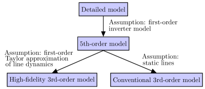
Figure 1: Detailed average model and reduced-order models with associated assumptions.

III-A System description

For the comparison analysis we consider the smallest unit and basic building block of larger microgrids, which is a typical two-inverter setup depicted by Fig. 2. Our justification for using this setup is based on the fact that reduced-order models that do not correctly predict stability for this basic configuration would also not be expected to perform better in the stability assessment of larger microgrids. In this test system (Fig. 2) each inverter is equipped with active power based frequency droop control, and reactive power based voltage droop control (a widely used control policy as in e.g. [10, 9, 19, 12, 49, 51, 44, 52, 53, 54, 17, 18, 20, 21]). The inverters are connected to buses $i,k$ respectively via a balanced resistive-inductive line defined by the line parameters $R_{ik},L_{ik}\in\mathbb{R}_{>0}$. Two local resistive-inductive (RL) loads $R_{\ell i},L_{\ell i}\in\mathbb{R}_{>0}$ and $R_{\ell k},L_{\ell k}\in\mathbb{R}_{>0}$ are connected to buses $i,k$ respectively. Fig. 3 shows that the output of an inverter is fitted with an $LC$ filter with parameters $R_{f},L_{f},C_{f}\in\mathbb{R}_{>0}$. This attenuates the harmonics that are introduced into the output voltage by the pulse-width modulation scheme. The voltage across the capacitor $v_{oi}$ (respectively $v_{ok}$) determines the voltage of bus $i$ (respectively $k$).

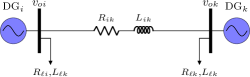
Figure 2: Two-inverter based autonomous microgrid

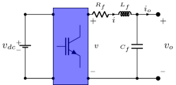
Figure 3: Schematic diagram of an AC inverter

The analysis in the rest of the paper is as follows. In section IV we provide a detailed description of the various models and derive those from first principles.

In section VI we evaluate the accuracy with which the reduced order models predict stability and instability. In particular, we find the range of values of the frequency and voltage droop gains for which each model is stable. These are then compared to those of the detailed average model, for different line $R/X$ ratios. Dynamic simulations of more advanced switching models are also presented for further validation. Our findings demonstrate significant discrepancies in the stability predictions of the reduced-order models and detailed average model, and further discussion on this is included in section VII.

IV Autonomous Microgrid Dynamic Models

In this section we describe in detail the models outlined in the previous section. In particular, in order to provide intuition on their relative merits, these are rigourously derived from first principles stating throughout the approximations made for the simpler models to be deduced.

IV-A Detailed Average Model

The detailed average model we consider in our study consists of all the internal states of an inverter, and the interconnection dynamics [10]. The inverter model uses the following standard assumptions: the DC-side (Fig. 3) is equipped with sufficient energy reserves; and a sufficiently high switching frequency allows to neglect the switching process. These allow the inverter dynamics to be described by a continuous average model which for convenience is formulated in the local $dq$ reference frame (Definition 3). In particular, the LC filter (Fig. 3) equations for inverter $i$ (respectively $k$) are obtained by applying $T(\theta_{i})$ with $\dot{\theta}_{i}=\omega_{i}$ to the fundamental inductor and capacitor equations (e.g., [10, 55]) to give:

$$L_{fi}\dot{i}_{dqi} = \omega_{i}L_{fi}{J}i_{dqi}-R_{fi}i_{dqi}+v_{dqi}-v_{o{dqi}}$$ (9)

$$C_{fi}\dot{v}_{o{dqi}} = \omega_{i}C_{fi}{J}v_{o{dqi}}+i_{dqi}-i_{o{dqi}}$$ (10)

where signals $i_{dqi}=[i_{di}~{}i_{qi}]^{\top}$, $i_{odqi}=[i_{odi}~{}i_{oqi}]^{\top}$, $v_{dqi}=[v_{di}~{}v_{qi}]^{\top}$, $v_{odqi}=[v_{odi}~{}v_{oqi}]^{\top}$ take values in $\mathbb{R}^{2}$ and are the inverter $dq$ currents and voltages of the form described by (3); $\omega_{i}$ is the inverter local frequency and takes value in $\mathbb{R}_{>0}$. The inverter frequency and voltage set points are specified via the frequency and voltage droop controllers, which for inverter $i$ (respectively $k$) are given by [10, 44]:

$$\small\tau\dot{\omega}_{i}= -\omega_{i}+\omega_{n}-k_{pi}P_{i}$$ (11a)

$$\tau\dot{V}_{i}= -V_{i}+V_{n}-k_{qi}Q_{i}$$ (11b)

where $V_{i}$ is the inverter voltage amplitude and takes value in $\mathbb{R}_{>0}$; $\tau,\omega_{n},V_{n},k_{pi},k_{qi}\in\mathbb{R}_{>0}$ are respectively the filtering time constant, nominal frequency, nominal voltage, frequency and voltage droop gains; $P_{i}$ and $Q_{i}$ are the respective measured active and reactive power. The inverter output voltage $v_{odqi}$ is regulated to the voltage value set by (11b) via the control input $v_{dqi}$. This is obtained from the (outer) voltage and (inner) current controllers which are respectively described for inverter $i$ (respectively $k$) as follows [10, 26, 56, 55]:

$$\begin{split}\dot{\phi}_{dqi}=&\mathbf{e}V_{i}-v_{odqi}\\ \dot{\gamma}_{dqi}=&i_{dqi}^{ref}-i_{dqi}\\ i_{dqi}^{ref}=&K_{PVi}(\mathbf{e}V_{i}-v_{odqi})+K_{IVi}\phi_{dqi}\\ v_{dqi}=&K_{PCi}(i_{dqi}^{ref}-i_{dqi})+K_{ICi}\gamma_{dqi}+\omega_{i}L_{fi}Ji_{dqi}\end{split}$$ (12)

where $\phi_{dqi}=[\phi_{di}~{}\phi_{qi}]^{\top}$, $\gamma_{dqi}=[\gamma_{dqi}~{}\gamma_{dqi}]^{\top}$ are the states of the voltage and current controllers respectively and take values in $\mathbb{R}^{2}$; $K_{PVi},K_{IVi}\in\mathbb{R}_{>0}$ are the proportional and integral gain of the voltage controller respectively; $K_{PCi},K_{ICi}\in\mathbb{R}_{>0}$ are the proportional and integral gain of the current controller respectively; $i_{dqi}^{ref}=[i_{di}^{ref}~{}i_{qi}^{ref}]^{\top}$ is the reference current that the current controller tracks and takes values in $\mathbb{R}^{2}$.

To facilitate the interconnection of the inverters, it is convenient to transform the port variables to the $DQ$ frame. The $DQ$ frame rotates with the synchronous frequency $\omega_{0}$ to which the inverter frequencies $\omega_{i}$ $(\omega_{k})$ converge at steady state. Recalling Definition 4, the RL line (Fig. 2) dynamics are derived by applying $T(\theta_{0})$ to the fundamental inductor equation (e.g., [10]):

$$\begin{split}L_{ik}\dot{I}_{DQ,ik}=&-R_{ik}I_{DQ,ik}+\omega_{0}L_{ik}JI_{DQ,ik}\\ &+\mathcal{T}(\delta_{i})v_{odqi}-\mathcal{T}(\delta_{k})v_{odqk}\end{split}$$ (13)

where $I_{DQ,ik}=[I_{D,ik}~{}I_{Q,ik}]^{\top}$ is the line current and takes values in $\mathbb{R}^{2}$, and

$$\small\dot{\delta}_{i}=\omega_{i}-\omega_{0}.$$ (14)

where $\delta_{i}\in\mathbb{S}$ is the angle between the two reference frames.

The load connected to bus $i$ (respectively $k$) is considered as an RL load and described on the synchronous reference frame [10]:

$$L_{\ell i}\dot{I}_{DQ,\ell i}=(-R_{\ell i}\mathbf{I}_{2}+\omega_{0}JL_{\ell i})I_{DQ,\ell i}+\mathcal{T}(\delta_{i})v_{odqi}$$ (15)

where $I_{DQ,\ell i}=[I_{D,\ell i}~{}I_{Q,\ell i}]^{\top}$ is the load current and takes values in $\mathbb{R}^{2}$; $R_{\ell i},L_{\ell i}\in\mathbb{R}_{>0}$ are the load resistance and inductance respectively.

In order to obtain $P_{i}$ and $Q_{i}$ in (11), the active and reactive power drawn by the load and that transferred over the line are required. The power drawn by the load at bus $i$ (respectively $k$) is given by

$$\begin{split}P_{\ell i}=&I_{DQ,\ell i}^{\top}\mathcal{T}(\delta_{i})v_{odqi}\\ Q_{\ell i}=&I_{DQ,\ell i}^{\top}J\mathcal{T}(\delta_{i})v_{odqi}\end{split}$$ (16)

where $P_{\ell i}$, $Q_{\ell i}$ are the active and reactive power respectively. The active and reactive power flows over the line from bus $i$ to bus $k$ are given as

$$\begin{split}P_{ik}=&I_{DQ,ik}^{\top}\mathcal{T}(\delta_{i})v_{odqi}\\ Q_{ik}=&I_{DQ,ik}^{\top}J\mathcal{T}(\delta_{i})v_{odqi}.\end{split}$$ (17)

The power injected by inverter $i$ is then computed as:

$$\begin{split}P_{i}=&P_{\ell i}+P_{ik}=(I_{DQ,ik}+I_{DQ,\ell i})^{\top}\mathcal{T}(\delta_{i})v_{odqi}\\ Q_{i}=&Q_{\ell i}+Q_{ik}=(I_{DQ,ik}+I_{DQ,\ell i})^{\top}J\mathcal{T}(\delta_{i})v_{odqi}\end{split}$$

and can also be written as

$$\begin{split}P_{i}=&i_{odqi}^{\top}v_{odqi}=(I_{DQ,ik}+I_{DQ,\ell i})^{\top}\mathcal{T}(\delta_{i})v_{odqi}\\ Q_{i}=&i_{odqi}^{\top}Jv_{odqi}=(I_{DQ,ik}+I_{DQ,\ell i})^{\top}J\mathcal{T}(\delta_{i})v_{odqi}\end{split}$$ (18)

Recall that ${J}\mathcal{T}(\delta_{i})=\mathcal{T}(\delta_{i}){J}$ (Remark 2), thus it clearly follows from (18) that

$$i_{odqi}=\mathcal{T}^{-1}(\delta_{i})(I_{DQ,ik}+I_{DQ,\ell i}).$$ (19)

Hence the detailed average model is described by (9)–(14), (19), which is used together with the load equation (15), and injected power (18).

IV-B Electromagnetic 5th-Order Model

In the detailed average model presented in IV-A the voltage across the capacitor (Fig. 3) tracks a reference via the control action of the outer and inner controllers. The electromagnetic (EM) 5th-order model is formulated by making the assumption that the outer and inner controllers are tuned to be much faster than the droop controllers such that a fast tracking response is obtained. By this reasonable assumption (similarly applied in [19, 12, 51]), dynamics (9)-(10), (12) are neglected, and the inverter is considered as a voltage source which produces at its output (Fig. 2) a symmetric three-phase AC voltage $v_{oi}:\mathbb{R}_{>0}\to\mathbb{R}^{3}$ of the form

$$\small v_{{oi}}={V_{i}\begin{bmatrix}\sin(\theta_{i})\\ \sin(\theta_{i}-\frac{2\pi}{3})\\ \sin(\theta_{i}+\frac{2\pi}{3}))\end{bmatrix}}$$ (20)

where $\theta_{i}$ is the angle defined as $\dot{\theta}_{i}=\omega_{i}$, and $V_{i}$, $\omega$ are respectively the voltage amplitude and frequency and take values in $\mathbb{R}_{>0}$. Due to this symmetry, $\mathds{1}^{\top}_{3}v_{oi}=0$. Thus, according to (3), (20) becomes

$$v_{o{dq_{i}}}=T(\theta_{i})v_{oi}=\mathbf{e}V_{i}.$$ (21)

For interconnection with the network, it is convenient to map the inverter output voltage to the synchronous rotating reference frame (Remark 2) as follows:

$$\mathcal{T}(\delta_{i})v_{o{dq_{i}}}=\mathcal{T}(\delta_{i})\mathbf{e}V_{i}=\begin{bmatrix}\cos(\delta_{i})\\ \sin(\delta_{i})\end{bmatrix}V_{i}$$ (22)

Applying the model simplifications described above, the electromagnetic (EM) 5th-order model with three states relating to the $i^{th}$ (respectively $k^{th}$) inverter (i.e. $\delta_{i},\omega_{i},V_{i}$) and two states for the lines ($DQ$ components of current $I_{DQ,ik}$) [11, 19] is:

$$\dot{\delta}_{i}= \omega_{i}-\omega_{0}$$ (23a)

$$\tau\dot{\omega}_{i}= -\omega_{i}+\omega_{n}-k_{pi}P_{i}$$ (23b)

$$\tau\dot{V}_{i}= -V_{i}+V_{n}-k_{qi}Q_{i}$$ (23c)

$$L_{ik}\dot{I}_{D,ik}= -R_{ik}I_{D,ik}+\omega_{0}L_{ik}I_{Q,ik}+V_{i}\cos\delta_{i}-V_{k}\cos\delta_{k}$$ (23d)

$$L_{ik}\dot{I}_{Q,ik}= -R_{ik}I_{Q,ik}-\omega_{0}L_{ik}I_{D,ik}+V_{i}\sin\delta_{i}-V_{k}\sin\delta_{k}$$ (23e)

Considering (22) the load model (15) is rewritten as

$$L_{\ell i}\dot{I}_{DQ,\ell i}=(-R_{\ell i}\mathbf{I}_{2}+\omega_{0}JL_{\ell i})I_{DQ,\ell i}+\mathcal{T}(\delta_{i})\mathbf{e}V_{i}.$$ (24)

The injected power $P_{i}$, $Q_{i}$ in (23b)–(23c) are computed as $P_{i}=P_{\ell i}+P_{ik}$ and $Q_{i}=Q_{\ell i}+Q_{ik}$. Considering (22) we rewrite (16) to obtain the active and reactive power drawn by the load at bus $i$ (respectively $k$) as follows:

$$\small\begin{split}P_{\ell i}&=I^{\top}_{DQ,\ell i}\mathcal{T}(\delta_{i})\mathbf{e}V_{i}\\ Q_{\ell i}&=I^{\top}_{DQ,\ell i}J\mathcal{T}(\delta_{i})\mathbf{e}V_{i}.\end{split}$$ (25)

Note that various reduced-order models can differ based on the approximations asserted on the line dynamics which also affects how the power exchange $P_{ik},Q_{ik}$ are computed. For the EM 5th-order model which considers the lines dynamics (23d)–(23e), and the corresponding power flows over the line from bus $i$ to bus $k$ is given by:

$$\small\begin{split}P_{ik}&=I^{\top}_{DQ,ik}\mathcal{T}(\delta_{i})\mathbf{e}V_{i}\\ Q_{ik}&=I^{\top}_{DQ,ik}J\mathcal{T}(\delta_{i})\mathbf{e}V_{i}\end{split}$$ (26)

The injected power $P_{i}$, $Q_{i}$ are

$$\begin{split}P_{i}=&P_{\ell i}+P_{ik}=(I_{DQ,ik}+I_{DQ,\ell i})^{\top}\mathcal{T}(\delta_{i})\mathbf{e}V_{i}\\ Q_{i}=&Q_{\ell i}+Q_{ik}=(I_{DQ,ik}+I_{DQ,\ell i})^{\top}J\mathcal{T}(\delta_{i})\mathbf{e}V_{i}.\end{split}$$ (27)

The 5th-order model of an inverter is therefore given by (23), which is used together with (24), (27).

IV-C Conventional 3rd-Order Model

The conventional 3rd-order model uses the same assumptions on the inverter dynamics as the 5th order model (section IV-B), and hence the inverter dynamics are described by (23a)–(23c). The main difference between the 3rd-order and the 5th-order model comes from the approximations asserted on the line dynamics, which also affects how the power exchange $P_{ik},Q_{ik}$ are calculated. The conventional 3rd-order model uses a traditional power system assumption of a distinct timescale separation which allows the line dynamics to be neglected and the lines modelled statically. In particular, the conventional 3rd-order model uses the traditional quasi-stationary approximation (also referred to as zero-order approximation model) [39, 40, 41, 42, 43, 44]. This involves evaluating (23d)–(23e) at equilibrium and corresponds to setting the derivative terms $\dot{I}_{D,ik},\dot{I}_{Q,ik}$ to zero as follows:

$$\small 0= -R_{ik}I_{D,ik}+\omega_{0}L_{ik}I_{Q,ik}+V_{i}\cos\delta_{i}-V_{k}\cos\delta_{k}$$ (28a)

$$0= -R_{ik}I_{Q,ik}-\omega_{0}L_{ik}I_{D,ik}+V_{i}\sin\delta_{i}-V_{k}\sin\delta_{k}.$$ (28b)

For simplicity in the analysis (28) is expressed as a phasor. To do this rewrite (28) by multiplying (28b) with the complex number $j$ as follows

$$\small 0= -R_{ik}I_{D,ik}+\omega_{0}L_{ik}I_{Q,ik}+V_{i}\cos\delta_{i}-V_{k}\cos\delta_{k}$$ (29a)

$$0= -jR_{ik}I_{Q,ik}-j\omega_{0}L_{ik}I_{D,ik}+jV_{i}\sin\delta_{i}-jV_{k}\sin\delta_{k}.$$ (29b)

The summation of (29a) and (29b) gives:

$$\small I^{0}_{ik}=(R_{ik}+j\omega_{0}L_{ik})^{-1}(V_{i}e^{j\delta_{i}}-V_{k}e^{j\delta_{k}})$$ (30)

where $I^{0}_{ik}=I_{D,ik}+jI_{Q,ik}$ is the current phasor and the superscript $0$ denotes that it is calculated at zero-order approximation. The corresponding zero-order approximation of the active and reactive power exchange is obtained via the relationship

$$\small P^{0}_{ik}+jQ^{0}_{ik}=(I^{0}_{ik})^{*}V_{i}e^{j\delta_{i}}$$

and this simplifies to:

$$\small\begin{split}P^{0}_{ik}&=G_{ik}V^{2}_{i}-G_{ik}V_{i}V_{k}\cos(\delta_{i}-\delta_{k})+B_{ik}V_{i}V_{k}\sin(\delta_{i}-\delta_{k})\\ Q^{0}_{ik}&=B_{ik}V^{2}_{i}-B_{ik}V_{i}V_{k}\cos(\delta_{i}-\delta_{k})-G_{ik}V_{i}V_{k}\sin(\delta_{i}-\delta_{k})\end{split}$$ (31)

where

$$\small G_{ik}=\frac{R_{ik}}{R^{2}_{ik}+X^{2}_{ik}},~{}~{}B_{ik}=\frac{X_{ik}}{R^{2}_{ik}+X^{2}_{ik}},~{}X_{ik}=\omega_{0}L_{ik},$$

$G_{ik},B_{ik},X_{ik}\in\mathbb{R}_{>0}$ are the conductance, susceptance and reactance respectively.

The injected power $P_{i}$, $Q_{i}$ are computed as

$$\begin{split}P_{i}=&P_{\ell i}+P_{ik}^{0}\\ Q_{i}=&Q_{\ell i}+Q_{ik}^{0}\end{split}$$ (32)

where $P_{\ell i}$, $Q_{\ell i}$ are given by (25), and $P_{ik}^{0}$, $Q_{ik}^{0}$ obtained from (31).
Hence the conventional 3rd-order model is described by (23a)–(23c), (31), which is used together with (24)–(25), (32).

IV-D High-Fidelity 3rd-Order Model

The high-fidelity 3rd-order model was proposed in [11] to improve the conventional 3rd-order model. The authors in [11] raised the concern that the inherent low inertia of inverters may not allow for straight-forward assumption of neglecting the line dynamics. The fast dynamics of lines can influence the slow ones despite their short timescale. This is in contrast to conventional power systems where a distinct timescale separation exists.

Below we describe the high-fidelity 3rd-order model following its derivation in [11]; in the description we relax the assumption that an inverter is connected to a fixed voltage bus. The high-fidelity 3rd-order model uses the same assumptions on the inverter dynamics as the 5th order model (section IV-B), and hence inverter dynamics are described by (23a)–(23c). The distinction between the high-fidelity 3rd-order model and the other two reduced-order models comes from the approximations asserted on the line dynamics, which also affects how the power exchange $P_{ik},Q_{ik}$ are computed. Instead of setting the derivative terms $\dot{I}_{D,ik},\dot{I}_{Q,ik}$ in (23d) and (23e) to zero, we take Laplace transforms which leads to the following:

$$\small sL_{ik}I_{D,ik}= -R_{ik}I_{D,ik}+\omega_{0}L_{ik}I_{Q,ik}+V_{i}\cos\delta_{i}$$

$$-V_{k}\cos\delta_{k}$$ (33a)

$$sL_{ik}I_{Q,ik}= -R_{ik}I_{Q,ik}-\omega_{0}L_{ik}I_{D,ik}+V_{i}\sin\delta_{i}$$

$$-V_{k}\sin\delta_{k}$$ (33b)

For convenience in the analysis we rewrite (33) by multiplying (33) with the complex number $j$ to obtain

$$\small sL_{ik}I_{D,ik}= -R_{ik}I_{D,ik}+\omega_{0}L_{ik}I_{Q,ik}+V_{i}\cos\delta_{i}$$

$$-V_{k}\cos\delta_{k}$$ (34a)

$$jsL_{ik}I_{Q,ik}= -jR_{ik}I_{Q,ik}-j\omega_{0}L_{ik}I_{D,ik}+jV_{i}\sin\delta_{i}$$

$$-jV_{k}\sin\delta_{k}$$ (34b)

The summation of (34) and (34) gives

$$\small\begin{split}I^{1}_{ik}=&\frac{V_{i}e^{j\delta_{i}}-V_{k}e^{j\delta_{k}}}{R_{ik}+j\omega_{0}L_{ik}+sL_{ik}}\\ =&\frac{(R_{ik}+j\omega_{0}L_{ik})^{-1}(V_{i}e^{j\delta_{i}}-V_{k}e^{j\delta_{k}})}{1+\tfrac{sL_{ik}}{R_{ik}+j\omega_{0}L_{ik}}}\end{split}$$

and this can be simplified to

$$I^{1}_{ik}=\frac{I^{0}_{ik}}{1+\tfrac{sL_{ik}}{R_{ik}+j\omega_{0}L_{ik}}}$$ (35)

where $I^{1}_{ik}=I_{D,ik}+jI_{Q,ik}$ is the current phasor. For the derivation of the equivalent reduced-order model that captures the dynamics of the slow modes, a reasonable assumption is that $|\tfrac{L_{ik}}{R_{ik}+j\omega_{0}L_{ik}}|$ is sufficiently small compared to the electromagnetic time $\frac{L_{ik}}{R_{ik}}$ such that (35) is represented by the first-order approximation of the Taylor expansion as follows:

$$\small I^{1}_{ik}\approx I^{0}_{ik}-\frac{L_{ik}}{R_{ik}+j\omega_{0}L_{ik}}sI^{0}_{ik}.$$ (36)

Returning to the time domain (36) can be rewritten as

$$\small I^{1}_{ik}\approx I^{0}_{ik}-\frac{L_{ik}}{R_{ik}+j\omega_{0}L_{ik}}\dot{I}^{0}_{ik}$$ (37)

where $I^{0}_{ik}$ is as in (30), and the term $\dot{I}^{0}_{ik}$ reads

$$\small\dot{I}^{0}_{ik}=\dot{V}_{i}e^{j\delta_{i}}+jV_{i}\dot{\delta}_{i}e^{j\delta_{i}}-\dot{V}_{k}e^{j\delta_{k}}-jV_{k}\dot{\delta}_{k}e^{j\delta_{k}}.$$

The corresponding first-order approximation of the active and reactive power is obtained from

$$\small P^{1}_{ik}+jQ^{1}_{ik}\approx(I^{1}_{ik})^{*}V_{i}e^{j\delta_{i}}$$ (38)

which simplifies to:

$$\small\begin{split}P^{1}_{ik}\approx~{}&P^{0}_{ik}-G^{\prime}_{ik}V_{i}\dot{V}_{i}+G^{\prime}_{ik}V_{i}\dot{V}_{k}\cos(\delta_{i}-\delta_{k})\\ &+G^{\prime}_{ik}V_{i}V_{k}\dot{\delta}_{k}\sin(\delta_{i}-\delta_{k})-B^{\prime}V^{2}_{i}\dot{\delta}_{i}\\ &-B^{\prime}_{ik}V_{i}\dot{V}_{k}\sin(\delta_{i}-\delta_{k})+B^{\prime}_{ik}V_{i}V_{k}\dot{\delta}_{k}\cos(\delta_{i}-\delta_{k})\end{split}$$ (39)

$$\small\begin{split}Q^{1}_{ik}\approx~{}&Q^{0}_{ik}+G^{\prime}_{ik}V^{2}_{i}\dot{\delta}_{i}+G^{\prime}_{ik}V_{i}\dot{V}_{k}\sin(\delta_{i}-\delta_{k})\\ &-G^{\prime}_{ik}V_{i}V_{k}\dot{\delta}_{k}\cos(\delta_{i}-\delta_{k})-B^{\prime}V_{i}\dot{V}_{i}\\ &+B^{\prime}_{ik}V_{i}\dot{V}_{k}\cos(\delta_{i}-\delta_{k})+B^{\prime}_{ik}V_{i}V_{k}\dot{\delta}_{k}\sin(\delta_{i}-\delta_{k})\end{split}$$ (40)

where

$$G^{\prime}_{ik}=\frac{(R^{2}_{ik}-X^{2}_{ik})L_{ik}}{(R^{2}_{ik}+X^{2}_{ik})^{2}},~{}~{}B^{\prime}_{ik}=\frac{2R_{ik}X_{ik}L_{ik}}{(R^{2}_{ik}+X^{2}_{ik})^{2}},$$

$G^{\prime}_{ik}\in\mathbb{R}$, $B^{\prime}_{ik}\in\mathbb{R}_{>0}$ can be referred to as the subsynchronous conductance and susceptance [11]. Typical values of $G^{\prime}_{ik},B^{\prime}_{ik}$ are small, but could play an important role during the transient response of the voltages and angles. Note that $P^{0}_{ik}$, $Q^{0}_{ik}$ given by (31) in the conventional 3rd-order model can be recovered if $G^{\prime}_{ik},B^{\prime}_{ik}$ are set to zero.

The injected power $P_{i}$, $Q_{i}$ are computed as

$$\begin{split}P_{i}=&P_{\ell i}+P_{ik}^{1}\\ Q_{i}=&Q_{\ell i}+Q_{ik}^{1}\end{split}$$ (41)

where $P_{\ell i}$, $Q_{\ell i}$ are given by (25), and $P_{ik}^{1}$, $Q_{ik}^{1}$ obtained from (39), (40) respectively.
Hence dynamics (23a)–(23c), (39)–(40) describe the high-fidelity 3rd-order model and are used together with (24)–(25), (41).

TABLE I: Microgrid parameters

Description	Value
Inverter $i$, $k$	$R_{f}$ = 0.1 $\Omega$, $L_{f}$ = 5 mH, $C_{f}$= 50 $\mu$F,
	$k_{p}$ = 6 $\times$ $10^{-5}$, $k_{q}$ = 1.5 $\times$ $10^{-4}$, $K_{PV}$ = 5,
	$K_{IV}$ = 10, $K_{PC}$ = 5, $K_{IC}$ = 25,
	$\omega_{n}$ = 2$\pi$(50) rad/s, $\tau$ = 31.8 ms, $V_{n}$ = 311 V.
R/X ratios	R/X $\gg$ 1 : $R_{ik}$ = 641 m$\Omega$, $L_{ik}$ = 0.26 mH
	R/X $\approx$ 1 : $R_{ik}$ = 195 m$\Omega$, $L_{ik}$ = 0.61 mH
	R/X $\ll$ 1 : $R_{ik}$ = 0.4 $\Omega$, $L_{ik}$ = 7 mH
Loads	$R_{\ell i}$ = 20 $\Omega$, $R_{\ell k}$ = 40 $\Omega$, $L_{\ell i}$ = 15 mH, $L_{\ell k}$ = 40 mH

V Small-Signal Models

The stability analysis in our comparative study in section VI is based on a small signal analysis of the detailed average model and reduced-order models. In order to obtain the small-signal models, we linearized the nonlinear dynamics (section IV) around an equilibrium point $x^{s}\in\{\delta^{s}_{i},\omega_{0},V^{s}_{i},\phi^{s}_{dqi},\gamma^{s}_{dqi},i^{s}_{dqi},v^{s}_{odqi},I^{s}_{DQ,ik},I^{s}_{DQ,\ell i}\}$. The equilibrium points are obtained from simulations of the nonlinear models (section IV) in three different regimes of line $R/X$ ratios for the setup in Fig. 2. The system parameters are given in Table I. The small-signal linearization of the detailed average model and reduced-order models can be found in the Appendix.

VI Model Accuracy Assessment

In this section, we assess the quality of the EM 5th-order, conventional 3rd-order, and high-fidelity 3rd-order models via the comparison of their stability properties to those of the detailed average model (section IV-A).

VI-A Small-Signal Stability Prediction

For the comparison in this section we deduce the range of values of the frequency and voltage droop gains ($k_{p}$ , $k_{q}$ respectively) for which each of the models is stable. This is carried out by increasing the droop gains until instability occurs. We will refer to the range of values of the droop gains where stability is maintained as the stability region of the model. These regions are deduced for each model for three different values of the line $R/X$ ratios, and are compared to those of the detailed model, as a means of evaluating the accuracy of the reduced order models.

Stability is determined via a small signal analysis and the corresponding eigenloci are also presented. The $R/X$ ratio regimes considered are $R/X\gg 1$, $R/X\approx 1$, and $R/X\ll 1$ respectively, which are regimes encountered in microgrids.

It should be noted that the voltage and current control gains of the inverters in the detailed average model are tuned to obtain the best possible performance. This is to allow a fair comparison of the detailed average model with the reduced-order models. Also note that the tests described in this section were repeated for various inverter/load/line parameters and similar conclusions were obtained. For convenience in the presentation the results are presented for typical equilibrium points with the parameters as described within the paper.

We now present the comparison results. Figs. 4, 6, 8 show the stability region of each model in the three different $R/X$ regimes. In particular, the region to the left of the each of the curves are the values of the droop gains for which the corresponding model is stable. Note that in the legend of Figs. 4–9 detailed model refers to the detailed average model; 5th-order refers to the EM 5th-order model; 3rd-order refers to the conventional 3rd-order model; and Hf 3rd-order refers to the high-fidelity 3rd-order model.

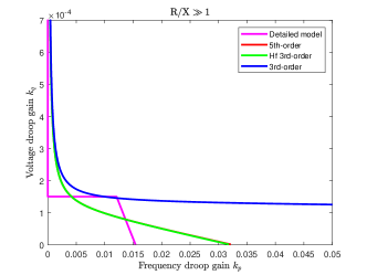
Figure 4: Comparison of stability regions given by the four small-signal models for the case $R/X\gg 1$. The region to the left of the corresponding curve are the values of the droop gains for which the model is stable.

.

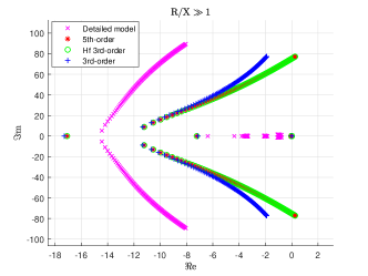
Figure 5: Eigenloci of the four small-signal models for the case $R/X\gg 1$ when $k_{pi}=k_{pk}$ take values in the range $[6\times 10^{-5},4.4\times 10^{-3}]$, and $k_{qi}=k_{qk}=1.5\times 10^{-4}$.

VI-A1 Line ratio $R/X\gg 1$

To investigate this regime we considered line parameters $R_{ik}=641~{}\text{m}\Omega$, $L_{ik}=0.26~{}\text{mH}$, $R/X\approx 7.8$ [57].

Stability Region

The stability region of the four models is presented in Fig. 4. It is evident that the 5th-order and high-fidelity 3rd-order models have the same stability region. Their stability region is greater than that of the detailed average model, but much smaller than that of the conventional 3rd-order model. Compared to the detailed average model, all the reduced-order models give erroneous stability results for large frequency and voltage droop gains. The conventional 3rd-order model, in particular, has the biggest discrepancy thus demonstrating that it is inappropriate for stability assessment when $R/X\gg 1$.

Eigenloci

Fig. 5 shows the eigenloci of each of the four models (i.e. the eigenvalues of state matrix $A$ in a state space representation). In particular, the eigenloci are plotted as the frequency droop coefficients $k_{pi}=k_{pk}$ vary in the interval $[6\times 10^{-5},4.4\times 10^{-3}]$. The voltage droop coefficients are set to $k_{qi}=k_{qk}=1.5\times 10^{-4}$ . It is clear that the eigenloci of the 5th-order and high-fidelity 3rd-order models are are very close, which confirms their similar stability regions (Fig. 4). It should also be noted that the location of the poles of the reduced-order models does not change much for large droop gains compared to that of the detailed average model. This causes the reduced models to give erroneous stability regions as was demonstrated in Fig. 4.

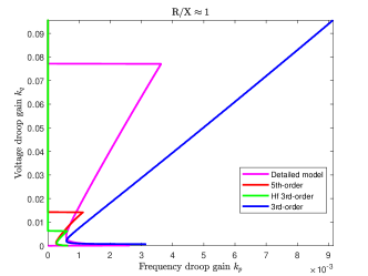
Figure 6: Comparison of stability regions given by the four small-signal models for the case $R/X\approx 1$. The region to the left of the corresponding curve are the values of the droop gains for which the model is stable.

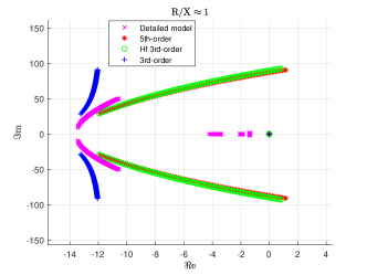
Figure 7: Eigenloci of the four small-signal models for the case $R/X\approx 1$ when $k_{pi}=k_{pk}$ take values in the range $[6\times 10^{-5},5.3\times 10^{-4}]$ and $k_{qi}=k_{qk}=1.5\times 10^{-4}$.

VI-A2 Line ratio $R/X\approx 1$

To investigate this regime we considered line parameters $R_{ik}=195~{}\text{m}\Omega$, $L_{ik}=0.61~{}\text{mH}$, $R/X\approx 1.0$ [11].

Stability Region

The stability region of each of the four models for the case $R/X\approx 1$ is presented in Fig. 6. The stability region of the high-fidelity 3rd-order is within that of the detailed average model. A similar behaviour is observed with the 5th-order model, but this admits a small error for some values of the frequency droop gain. The conventional 3rd-order model, differs from the detailed model (i.e. gives wrong stability results), for a large range of values of the droop gains. It should also be noted that the 5th-order and high-fidelity 3rd-order models show stability for only relatively a small range of values of the droop gains compared to those of the detailed average model.

Eigenloci

These are shown in Fig. 7 as the frequency droop coefficients $k_{pi}=k_{pk}$ vary in the interval $[6\times 10^{-5},5.3\times 10^{-4}]$. The voltage droop coefficients are set to $k_{qi}=k_{qk}=1.5\times 10^{-4}$ . The eigenloci of the 5th-order and high-fidelity 3rd-order models are very close, and show instability at lower values of the droop gains relative to those of the detailed average model. This also agrees with Fig. 6. There is also no significant change in the location of the poles of the conventional 3rd-order model for large droop gains, which confirms its poor performance in Fig. 6.

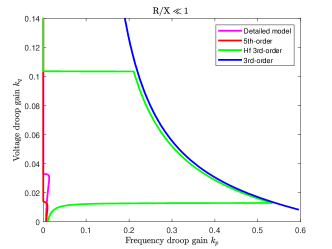
Figure 8: Comparison of stability regions predicted by the four small-signal models for the case $R/X\ll 1$. The region to the left of the corresponding curve are the values of the droop gains for which the model is stable.

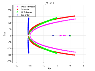
Figure 9: Eigenloci of the four small-signal models for the case $R/X\ll 1$ when $k_{pi}=k_{pk}$ take values in the range $[6\times 10^{-5},7\times 10^{-3}]$ and $k_{qi}=k_{qk}=1.5\times 10^{-4}$.

VI-A3 Line ratio $R/X\ll 1$

To investigate this regime we considered line parameters $R_{ik}=0.4~{}\Omega$, $L_{ik}=7~{}\text{mH}$, $R/X\approx 0.18$ [12, 19, 9].

Stability Region

These are presented in Fig. 8. It is evident that the stability region of the 5th-order model is reasonably within that associated with the detailed average model, while those of the 3rd order models are erroneous for a large range of values of the droop gains. This shows that the 3rd order models are highly unsuitable for stability assessment when $R/X\ll 1$.

Eigenloci

These are shown in Fig. 9 as the frequency droop coefficients $k_{pi}=k_{pk}$ vary in the interval $[6\times 10^{-5},7\times 10^{-3}]$. The voltage droop coefficients are set to $k_{qi}=k_{qk}=1.5\times 10^{-4}$. The eigenloci of the 5th-order and the detailed average model shows instability at lower values of the droop gains relative to those of the 3rd order models. The location of the poles of the conventional 3rd-order model does not change much for large droop gains, and hence incorrectly predicts stability in this regime as also shown in Fig. 8. The pole movement of the high-fidelity 3rd-order model better reflects that of the detailed model, in comparison with the conventional 3rd-order model. There is, however, error in its stability predictions for large droop gains.

VI-B Nonlinear Model Dynamic Response

In this section we present dynamic responses that demonstrate the stability results shown in Figs. 5, 7, 9 for the respective $R/X$ cases. The model used in the simulations is a more detailed one and includes the on/off actuation of the electronic switches via PWM. Figs. 10a, 11a, 12a show the responses when the lower value of the frequency droop gain used in Figs. 5, 7, 9 is chosen, which is $k_{pi}=k_{pk}=6\times 10^{-5}$. Likewise Figs. 10b, 11b, 12b show the responses when the upper values of the frequency droop gain used in Figs. 5, 7, 9 are chosen, which are $k_{pi}=k_{pk}=4.4\times 10^{-3}$, $5.3\times 10^{-4}$, $7\times 10^{-3}$ respectively.

It is evident in Figs. 10a, 11a, 12a that the reduced-order models produce stable responses which are similar to those of the detailed average model when the lower values of the frequency droop gains are used. This is expected as small droop gains do not cause instability (at the expense of a slower response). The responses presented in Figs. 10b, 11b, 12b, which demonstrate also unstable behaviour, agree with the stability results in Figs. 5, 7, 9 respectively. This further validates the veracity of the stability regions shown in Figs. 4, 6, 8.

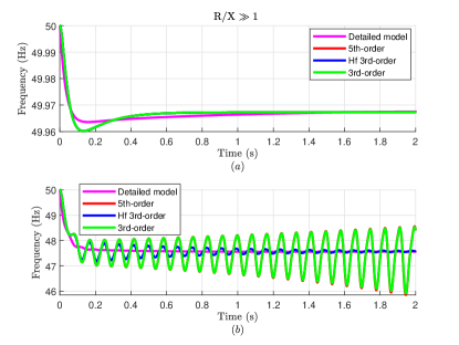
Figure 10: Dynamic responses of the four nonlinear models for the case $R/X\gg 1$ when: (a) $k_{pi}=k_{pk}=6\times 10^{-5}$, $k_{qi}=k_{qk}=1.5\times 10^{-4}$; (b) $k_{pi}=k_{pk}=4.4\times 10^{-3}$, $k_{qi}=k_{qk}=1.5\times 10^{-4}$.

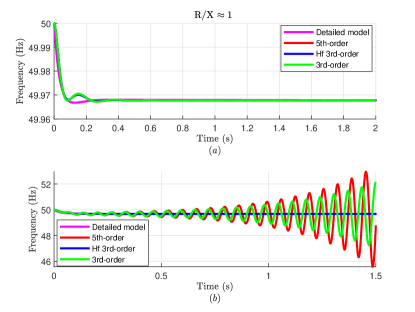
Figure 11: Dynamic responses of the four nonlinear models for the case $R/X\approx 1$ when: (a) $k_{pi}=k_{pk}=6\times 10^{-5}$, $k_{qi}=k_{qk}=1.5\times 10^{-4}$; (b) $k_{pi}=k_{pk}=5.3\times 10^{-4}$, $k_{qi}=k_{qk}=1.5\times 10^{-4}$.

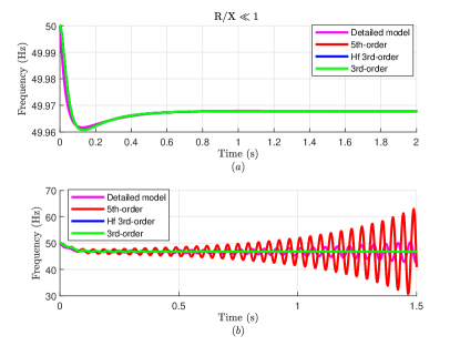
Figure 12: Dynamic responses of the four nonlinear models for the case $R/X\ll 1$ when: (a) $k_{pi}=k_{pk}=6\times 10^{-5}$, $k_{qi}=k_{qk}=1.5\times 10^{-4}$; (b) $k_{pi}=k_{pk}=7\times 10^{-3}$, $k_{qi}=k_{qk}=1.5\times 10^{-4}$.

VII Discussion

In this section we discuss the findings of the analysis in section VI and describe the relative merits of the models considered.

The small-signal stability analysis showed that the conventional 3rd-order model gives inaccurate stability results in all three regimes of the line $R/X$ ratio, and hence it cannot be recommended for stability analysis. The high-fidelity 3rd-order model performance is acceptable only when $R/X\approx 1$, and appears to be conservative, in the sense that it has a smaller stability region compared to that of the detailed average model. The 5th-order model generally performs better and admits small error in its stability results in all the cases except when $R/X\gg 1$.

The discrepancy observed in the stability results given by the reduced-order models relative to those of the detailed average model shows that neglecting the inverters’ current and voltage controller dynamics affects their stability properties. The additional omission of the line dynamics in the conventional 3rd-order model further explains its overall poor performance in all the cases, compared to that of the other two reduced-order models. This shows that line dynamics can play a vital role in microgrid stability analysis and should not in general be omitted.

The stablity of the the detailed average model for a smaller range of the droop gains when $R/X\gg 1$ suggests that the inverter’s voltage and current controllers, and their interaction with the line dynamics, play a key role in the stability of very resistive microgrids. This is consistent with the insight that when the $R/X$ value is large, the line dynamics become fast. Therefore their timescale overlaps that of the inverters’ voltage and current controllers, which causes their strong coupling. Since the reduced models have poor performance when $R/X\gg 1$, we recommend that the detailed average model is used in this case.

We also presented in section VI dynamic responses of the models considered and a comparison was also made with the responses of a more detailed switching model. The dynamic responses were consistent with the stability analysis and also validated the accuracy of the detailed average model.

Based on our findings, Table II summarises the accuracy of the three reduced-order models for predicting stability in the three $R/X$ regimes considered. We categorise this based on a descending scale of "Good", "Acceptable", and "Unacceptable". "Good" means that the stable region of the model is within that of the detailed average model, even though some conservatism may be present; "Acceptable" indicates that the associated stable region is generally within that of the detailed model, but there is a small error for some droop gains; "Unacceptable" implies that erroneous stability results are given for a large range of values of the droop gains (i.e., the corresponding stable region is larger than that of the detailed average model).

TABLE II: Stability Predictions of the Three Reduced-Order models

	$R/X\gg 1$	$R/X\approx 1$	$R/X\ll 1$
EM 5th-order	Unacceptable	Acceptable	Acceptable
Hf 3rd-order	Unacceptable	Good	Unacceptable
3rd-order	Unacceptable	Unacceptable	Unacceptable

Recommendations

It would be expected that the reduced-order models may admit some inaccuracies compared to the detailed average model in their stability properties. However, in order to avoid excessive discrepancies we present some brief recommendations on selecting an appropriate reduced order model, based on the results of our study.

• The high-fidelity 3rd-order and 5th-order models can be used in the case of line $R/X$ ratio close to unity.

• For inductive microgrids ($R/X\ll 1$) we recommend that only the 5th-order model can be used.

• We caution the use of reduced-order models that aim to simplify the inverter and line dynamics in the case of very resistive microgrids ($R/X\gg 1$). The detailed average model is still though an appropriate model in this regime.

VIII Conclusion

Reduced order dynamic models for microgrids have been extensively used in the literature so as to facilitate system-wide stability assessment and analytical studies. The simplifications inevitably present in the reduced-order models raise the concern over the correctness of their stability properties compared to those of more detailed average models. Their performance also differs in different regimes of the line $R/X$ ratios as the latter is associated with the timescale of the line dynamics and the extent to which these interfere with the dynamics of the inverters.

We have therefore conducted a comprehensive comparative study of the accuracy of the following commonly used reduced order models: the electromagnetic 5th-order, the conventional 3rd-order, and a high-fidelity 3rd-order model. A comparison has been made of the stability predictions of these models to those of a detailed average model for various regimes of the line $R/X$ ratios. Our study has demonstrated that the 3rd-order model, where line dynamics are omited, can provide inaccurate stability results in all three regimes of the line $R/X$ ratios. The accuracy of the high-fidelity 3rd-order model degrades as the $R/X$ ratio becomes either very large or small, and the electromagnetic 5th-order becomes inaccurate when the $R/X$ ratio is very large.

Therefore the 5th-order and the high-fidelity 3rd-order models appear to be appropriate for microgrids with $R/X$ close to unity, and the former appears to be also quite accurate when the microgrid is inductive. We strongly advise caution when using reduced-order models in highly resistive microgrids.

Appendix A Detailed Average Model

In order to present the small-signal linearized model, we introduce the error states: $\tilde{\delta}_{i}=\delta_{i}-\delta^{s}_{i}$, $\tilde{\omega}_{i}=\omega_{i}-\omega_{0}$, $\tilde{V}_{i}=V_{i}-V^{s}_{i}$, $\tilde{\phi}_{dqi}=\phi_{dqi}-\phi^{s}_{dqi}$, $\tilde{\gamma}_{dqi}=\gamma_{dqi}-\gamma^{s}_{dqi}$, $\tilde{v}_{odqi}=v_{odqi}-v^{s}_{odqi}$, $\tilde{I}_{DQ,ik}=I_{DQ,ik}-I^{s}_{DQ,ik}$, $\tilde{I}_{DQ,\ell i}=I_{DQ,\ell i}-I^{s}_{DQ,\ell i}$.

The entries of the Jacobian matrix for the detailed average model are defined as follows: Let $r=i,k$, $\Lambda_{p}=\text{diag}\left(\frac{1}{k_{pi}},\frac{1}{k_{pk}}\right)$, $\Lambda_{q}=\text{diag}\left(\frac{1}{k_{qi}},\frac{1}{k_{qk}}\right)$, $\sigma=\text{diag}(\mathbf{e},\mathbf{e})$, $\sigma^{v}_{kp}=\text{diag}(K_{PVi}\mathbf{e},K_{PVk}\mathbf{e})$, $\sigma^{cv}_{kp}=\text{diag}(K_{PVi}K_{PCi}\mathbf{e},K_{PVk}K_{PCk}\mathbf{e})$, $K_{PV}=\text{diag}(K_{PVi}\mathbf{I}_{2},K_{PVk}\mathbf{I}_{2})$, $K_{IV}=\text{diag}(K_{IVi}\mathbf{I}_{2},K_{IVk}\mathbf{I}_{2})$, $K_{IC}=\text{diag}(K_{ICi}\mathbf{I}_{2},K_{ICk}\mathbf{I}_{2})$, $\sigma^{v}=\text{diag}(\sigma^{v}_{i},\sigma^{v}_{k}),\sigma^{v}_{r}=K_{PCr}K_{PVr}\mathbf{I}_{2}+\mathbf{I}_{2}$, $\sigma_{pc}=\text{diag}(K_{PCi}K_{IVi}\mathbf{I}_{2},K_{PCk}K_{IVk}\mathbf{I}_{2})$, $\mathcal{Z}_{f}=\text{diag}(Z_{fi},Z_{fk})\in\mathbb{R}^{4\times 4}$, $Z_{fr}=-R_{fr}\mathbf{I}_{2}+2\omega_{0}JL_{fr}-K_{PCr}\mathbf{I}_{2}$, $Z_{fv}=\text{diag}(\omega_{0}C_{fi}J,\omega_{0}C_{fk}J)$, $\mathcal{Z}_{\ell}=\text{diag}(Z_{i},Z_{k})\in\mathbb{R}^{4\times 4}$, $Z_{r}=-R_{\ell r}\mathbf{I}_{2}+\omega_{0}JL_{\ell r},\mathcal{Z}_{ik}=-R_{ik}\mathbf{I}_{2}+\omega_{0}JL_{ik}$, $N=\begin{bmatrix}-\mathcal{T}(\delta^{s}_{i})~{}\mathcal{T}(\delta^{s}_{k})\end{bmatrix}^{\top}$, $N^{\delta}=\text{diag}(-\frac{\partial{\mathcal{T}^{-1}(\delta^{s}_{i})}}{\partial\delta_{i}}I^{s}_{DQ,ik},\frac{\partial{\mathcal{T}^{-1}(\delta^{s}_{k})}}{\partial\delta_{k}}I^{s}_{DQ,ik})$, $N_{\ell}=\text{diag}(\mathcal{T}(\delta^{s}_{i})^{-1},\mathcal{T}(\delta^{s}_{k})^{-1})$, $C_{f}=\text{diag}(C_{fi}\mathbf{I}_{2},C_{fk}\mathbf{I}_{2})$, $N^{\delta}_{\ell}=\text{diag}(\frac{\partial{\mathcal{T}^{-1}(\delta^{s}_{i})}}{\partial\delta_{i}}I^{s}_{DQ\ell i},\frac{\partial{\mathcal{T}^{-1}(\delta^{s}_{k})}}{\partial\delta_{k}}I^{s}_{DQ\ell k})$, $\mathcal{N}^{v}=\text{diag}(\mathcal{T}(\delta^{s}_{i}),\mathcal{T}(\delta^{s}_{k}))$,
$\mathcal{N}^{\delta}=\text{diag}(\frac{\partial{\mathcal{T}(\delta^{s}_{i})}}{\partial\delta_{i}}v^{s}_{odqi},\frac{\partial{\mathcal{T}(\delta^{s}_{k})}}{\partial\delta_{k}}v^{s}_{odqk})$, $\mathcal{D}^{I}_{\omega}=2\times\text{diag}(L_{fi}Ji^{s}_{dqi},L_{fk}Ji^{s}_{dqk})$, $L_{\ell}=\text{diag}(L_{\ell i}\mathbf{I}_{2},L_{\ell k}\mathbf{I}_{2})$, $\mathcal{D}^{v}_{\omega}=\text{diag}(C_{fi}Jv^{s}_{odqi},C_{fk}Jv^{s}_{odqk})$, $\mathcal{\bar{N}}^{\delta}=\begin{bmatrix}\frac{\partial{\mathcal{T}(\delta^{s}_{i})}}{\partial\delta_{i}}v^{s}_{odqi}~{}-\frac{\partial{\mathcal{T}(\delta^{s}_{k})}}{\partial\delta_{k}}v^{s}_{odqk}\end{bmatrix}$, $\mathcal{N}=\begin{bmatrix}\mathcal{T}(\delta^{s}_{i})~{}-\mathcal{T}(\delta^{s}_{k})\end{bmatrix}$, $\frac{\partial P}{\partial v_{odq}}=\text{diag}(\frac{\partial P_{i}}{\partial v_{odqi}}\Bigr{|}_{x^{s}},\frac{\partial P_{k}}{\partial v_{odqk}}\Bigr{|}_{x^{s}}),\bar{N}=N^{\delta}-N^{\delta}_{\ell}$, $\frac{\partial Q}{\partial v_{odq}}=\text{diag}(\frac{\partial Q_{i}}{\partial v_{odqi}}\Bigr{|}_{x^{s}},\frac{\partial Q_{k}}{\partial v_{odqk}}\Bigr{|}_{x^{s}})$, $L_{f}=\text{diag}(L_{fi}\mathbf{I}_{2},L_{fk}\mathbf{I}_{2})$, $\mathcal{D}^{q}_{\ell}=\text{diag}(D_{i},D_{k})\in\mathbb{R}^{2\times 4},D_{r}=\begin{bmatrix}\frac{\partial Q_{r}}{\partial I_{D,\ell r}}\Bigr{|}_{x^{s}}&\frac{\partial Q_{r}}{\partial I_{Q,\ell r}}\Bigr{|}_{x^{s}}\end{bmatrix}$, $\mathcal{D}^{p}_{\ell}=\text{diag}(\bar{D}_{i},\bar{D}_{k})\in\mathbb{R}^{2\times 4}$, $\bar{D}_{r}=\begin{bmatrix}\frac{\partial P_{r}}{\partial I_{D,\ell r}}\Bigr{|}_{x^{s}}&\frac{\partial P_{r}}{\partial I_{Q,\ell r}}\Bigr{|}_{x^{s}}\end{bmatrix}$, $\frac{\partial P}{\partial\delta}=\text{diag}\left(\frac{\partial P_{i}}{\partial\delta_{i}}\Bigr{|}_{x^{s}},\frac{\partial P_{k}}{\partial\delta_{k}}\Bigr{|}_{x^{s}}\right)$, $\frac{\partial Q}{\partial\delta}=\text{diag}\left(\frac{\partial Q_{i}}{\partial\delta_{i}}\Bigr{|}_{x^{s}},\frac{\partial Q_{k}}{\partial\delta_{k}}\Bigr{|}_{x^{s}}\right)$, $\frac{\partial P}{\partial I_{DQ,ik}}=\begin{bmatrix}\frac{\partial P_{i}}{\partial I_{D,ik}}\Bigr{|}_{x^{s}}&\frac{\partial P_{i}}{\partial I_{Q,ik}}\Bigr{|}_{x^{s}}\\ \frac{\partial P_{k}}{\partial I_{D,ik}}\Bigr{|}_{x^{s}}&\frac{\partial P_{k}}{\partial I_{Q,ik}}\Bigr{|}_{x^{s}}\end{bmatrix}$, $\frac{\partial Q}{\partial I_{DQ,ik}}=\begin{bmatrix}\frac{\partial Q_{i}}{\partial I_{D,ik}}\Bigr{|}_{x^{s}}&\frac{\partial Q_{i}}{\partial I_{Q,ik}}\Bigr{|}_{x^{s}}\\ \frac{\partial Q_{k}}{\partial I_{D,ik}}\Bigr{|}_{x^{s}}&\frac{\partial Q_{k}}{\partial I_{Q,ik}}\Bigr{|}_{x^{s}}\end{bmatrix}$,
$\Gamma=\text{diag}(\mathbf{I}_{2},\tau\Lambda_{p},\tau\Lambda_{q},\mathbf{I}_{4},\mathbf{I}_{4},L_{f},C_{f},L_{ik}\mathbf{I}_{2},L_{\ell})\in\mathbb{R}^{28\times 28}$.

The small-signal state space model of the detailed average model is described by (42):

$$\dot{\tilde{x}}=\Gamma^{-1}\begin{bmatrix}A_{11}&A_{12}\\ A_{21}&A_{22}\end{bmatrix}\tilde{x}$$ (42)

where

$$\tilde{x}=[\tilde{\delta}_{i},\tilde{\delta}_{k},\tilde{\omega}_{i},\tilde{\omega}_{k},\tilde{\phi}^{\top}_{dqi},\tilde{\phi}^{\top}_{dqk},\tilde{\gamma}^{\top}_{dqi},\tilde{\gamma}^{\top}_{dqk},\tilde{i}^{\top}_{dqi},\tilde{i}^{\top}_{dqk},$$

$$\tilde{v}^{\top}_{odqi},\tilde{v}^{\top}_{odqk},\tilde{I}^{\top}_{DQ,ik},\tilde{I}^{\top}_{DQ,\ell i},\tilde{I}^{\top}_{DQ,\ell k}]^{\top}$$

$A_{11}=\begin{bmatrix}0&\mathbf{I}_{2}&0&0&0&0\\ -\frac{\partial P}{\partial\delta}&-\Lambda_{p}&0&0&0&0\\ -\frac{\partial Q}{\partial\delta}&0&-\Lambda_{q}&0&0&0\\ 0&0&\sigma&0&0&0\\ 0&0&\sigma^{v}_{kp}&K_{IV}&0&-\mathbf{I}_{4}\\ 0&\mathcal{D}^{I}_{\omega}&\sigma^{cv}_{kp}&\sigma_{pc}&K_{IC}&Z_{f}\end{bmatrix}$
$A_{12}=\begin{bmatrix}0&0&0\\ -\frac{\partial P}{\partial v_{odq}}&-\frac{\partial P}{\partial I_{DQ,ik}}&-\mathcal{D}^{p}_{\ell}\\ -\frac{\partial Q}{\partial v_{odq}}&-\frac{\partial Q}{\partial I_{DQ,ik}}&-\mathcal{D}^{q}_{\ell}\\ -\mathbf{I}_{4}&0&0\\ -K_{PV}&0&0\\ -\sigma^{v}&0&0\\ \end{bmatrix}$
$A_{21}=\begin{bmatrix}\bar{N}&\mathcal{D}^{v}_{\omega}&0&0&0&\mathbf{I}_{4}\\ \mathcal{\bar{N}}^{\delta}&0&0&0&0&0\\ \mathcal{N}^{\delta}&0&0&0&0&0\end{bmatrix}$
$A_{22}=\begin{bmatrix}Z_{fv}&N&-N_{\ell}\\ \mathcal{N}&\mathcal{Z}_{ik}&0\\ \mathcal{N}^{v}&0&\mathcal{Z}_{\ell}\end{bmatrix}$
$\tilde{x}\in\mathbb{R}^{28},A\in\mathbb{R}^{28\times 28}$.

Appendix B EM 5th-Order Small-Signal Model

The entries of the Jacobian matrix for the EM 5th-order model are defined as follows:
$\mathcal{M}^{\delta}_{\ell}=\text{diag}(\frac{\partial{\mathcal{T}(\delta^{s}_{i})}}{\partial\delta_{i}}\mathbf{e}V^{s}_{i},\frac{\partial{\mathcal{T}(\delta^{s}_{k})}}{\partial\delta_{k}}\mathbf{e}V^{s}_{k})$,
$\mathcal{M}^{v}=[\mathcal{T}(\delta_{i})\mathbf{e}~{}-\mathcal{T}(\delta_{k})\mathbf{e}]$,
$\mathcal{M}^{v}_{\ell}=\text{diag}(\mathcal{T}(\delta_{i})\mathbf{e},\mathcal{T}(\delta_{k})\mathbf{e})$,
$\mathcal{M}^{\delta}=[\frac{\partial{\mathcal{T}(\delta^{s}_{i})}}{\partial\delta_{i}}\mathbf{e}V^{s}_{i}~{}-\frac{\partial{\mathcal{T}(\delta^{s}_{k})}}{\partial\delta_{k}}\mathbf{e}V^{s}_{k}]$, $\frac{\partial P}{\partial V}=\text{diag}(\frac{\partial P_{i}}{\partial V_{i}}\Bigr{|}_{x^{s}},\frac{\partial P_{k}}{\partial V_{k}}\Bigr{|}_{x^{s}})$, $\frac{\partial Q}{\partial V}=\text{diag}(\frac{\partial Q_{i}}{\partial V_{i}}\Bigr{|}_{x^{s}},\frac{\partial Q_{k}}{\partial V_{k}}\Bigr{|}_{x^{s}})$,
$\Gamma_{5}=\text{diag}(\mathbf{I}_{2},\tau\Lambda_{p},\tau\Lambda_{q},L_{ik}\mathbf{I}_{2},L_{\ell})\in\mathbb{R}^{12\times 12}$.

The 5th-order small-signal state space model is described by (43):

$$\dot{\tilde{x}}_{5}=\Gamma_{5}^{-1}A_{5}\tilde{x}_{5}$$ (43)

where $\tilde{x}_{5}=[\tilde{\delta}_{i},\tilde{\delta}_{k},\tilde{\omega}_{i},\tilde{\omega}_{k},\tilde{V}_{i},\tilde{V}_{k},\tilde{I}^{\top}_{DQ,ik},\tilde{I}^{\top}_{DQ,\ell i},\tilde{I}^{\top}_{DQ,\ell k}]^{\top},$

$$\scriptsize A_{5}=\begin{bmatrix}\mymathbb{0}_{2\times 2}&\mathbf{I}_{2}&\mymathbb{0}_{2\times 2}&\mymathbb{0}_{2\times 2}&\mymathbb{0}_{2\times 4}\\ -\frac{\partial P}{\partial\delta}&-\Lambda_{p}&-\frac{\partial P}{\partial V}&-\frac{\partial P}{\partial I_{dq,ik}}&-\mathcal{D}^{p}_{\ell}\\ -\frac{\partial Q}{\partial\delta}&\mymathbb{0}_{2\times 2}&-(\Lambda_{q}+\frac{\partial Q}{\partial V})&-\frac{\partial Q}{\partial I_{dq,ik}}&-\mathcal{D}^{q}_{\ell}\\ \mathcal{M}^{\delta}&\mymathbb{0}_{2\times 2}&\mathcal{M}^{v}&\mathcal{Z}_{ik}&\mymathbb{0}_{2\times 4}\\ \mathcal{M}^{\delta}_{\ell}&\mymathbb{0}_{4\times 2}&\mathcal{M}^{v}_{\ell}&\mymathbb{0}_{4\times 2}&\mathcal{Z}_{\ell}\end{bmatrix},$$

$\tilde{x}_{5}\in\mathbb{R}^{12},A_{5}\in\mathbb{R}^{12\times 12}$. Other entries in $\Gamma_{5},A_{5}$ are as defined in Appendix A

Appendix C Conventional 3rd-Order Small-Signal Model

The following are defined to present the Jacobian matrix of the 3rd-order small-signal model:
$\mathcal{D}^{p}_{\delta}=\begin{bmatrix}\frac{\partial P_{i}}{\partial\delta_{i}}\Bigr{|}_{x^{s}}&\frac{\partial P_{i}}{\partial\delta_{k}}\Bigr{|}_{x^{s}}\\ \frac{\partial P_{k}}{\partial\delta_{i}}\Bigr{|}_{x^{s}}&\frac{\partial P_{k}}{\partial\delta_{k}}\Bigr{|}_{x^{s}}\end{bmatrix}$, $\mathcal{D}^{q}_{\delta}=\begin{bmatrix}\frac{\partial Q_{i}}{\partial\delta_{i}}\Bigr{|}_{x^{s}}&\frac{\partial Q_{i}}{\partial\delta_{k}}\Bigr{|}_{x^{s}}\\ \frac{\partial Q_{k}}{\partial\delta_{i}}\Bigr{|}_{x^{s}}&\frac{\partial Q_{k}}{\partial\delta_{k}}\Bigr{|}_{x^{s}}\end{bmatrix}$,
$\mathcal{D}^{p}_{v}=\begin{bmatrix}\frac{\partial P_{i}}{\partial V_{i}}\Bigr{|}_{x^{s}}&\frac{\partial P_{i}}{\partial V_{k}}\Bigr{|}_{x^{s}}\\ \frac{\partial P_{k}}{\partial V_{i}}\Bigr{|}_{x^{s}}&\frac{\partial P_{k}}{\partial V_{k}}\Bigr{|}_{x^{s}}\end{bmatrix}$, $\mathcal{D}^{q}_{v}=\begin{bmatrix}\frac{\partial Q_{i}}{\partial V_{i}}\Bigr{|}_{x^{s}}&\frac{\partial Q_{i}}{\partial V_{k}}\Bigr{|}_{x^{s}}\\ \frac{\partial Q_{k}}{\partial V_{i}}\Bigr{|}_{x^{s}}&\frac{\partial Q_{k}}{\partial V_{k}}\Bigr{|}_{x^{s}}\end{bmatrix}$,
$\Gamma_{3}=\text{diag}(\mathbf{I}_{2},\tau\Lambda_{p},\tau\Lambda_{q},L_{\ell})\in\mathbb{R}^{10\times 10}$.

The conventional 3th-order small-signal state space model is described by (44):

$$\dot{\tilde{x}}_{3}=\Gamma_{3}^{-1}A_{3}\tilde{x}_{3}$$ (44)

where $\tilde{x}_{3}=[\tilde{\delta}_{i},\tilde{\delta}_{k},\tilde{\omega}_{i},\tilde{\omega}_{k},\tilde{V}_{i},\tilde{V}_{k},\tilde{I}^{\top}_{dq,\ell i},\tilde{I}^{\top}_{dq,\ell k}]^{\top},$

$$\scriptsize A_{3}=\begin{bmatrix}\mymathbb{0}_{2\times 2}&\mathbf{I}_{2}&\mymathbb{0}_{2\times 2}&\mymathbb{0}_{2\times 4}\\ -\mathcal{D}^{p}_{\delta}&-\Lambda_{p}&-\mathcal{D}^{p}_{v}&-\mathcal{D}^{p}_{\ell}\\ -\mathcal{D}^{q}_{\delta}&\mymathbb{0}_{2\times 2}&-(\Lambda_{q}+\mathcal{D}^{q}_{v})&-\mathcal{D}^{q}_{\ell}\\ \mathcal{M}^{\delta}_{\ell}&\mymathbb{0}_{4\times 2}&\mathcal{M}^{v}_{\ell}&\mathcal{Z}_{\ell}\end{bmatrix},$$

$\tilde{x}_{3}\in\mathbb{R}^{10},A_{3}\in\mathbb{R}^{10\times 10}$. Other entries in $\Gamma_{\text{3}},A_{3}$ are as defined in Appendixes A and B respectively.

Appendix D High-Fidelity 3rd-Order Small-Signal Model

We define the following to present the Jacobian matrix of the high-fidelity 3rd-order small-signal model:
$\mathcal{D}^{p}_{\omega}=\begin{bmatrix}\frac{\partial P_{i}}{\partial\dot{\delta}_{i}}\Bigr{|}_{x^{s}}&\frac{\partial P_{i}}{\partial\dot{\delta}_{k}}\Bigr{|}_{x^{s}}\\ \frac{\partial P_{k}}{\partial\dot{\delta}_{i}}\Bigr{|}_{x^{s}}&\frac{\partial P_{k}}{\partial\dot{\delta}_{k}}\Bigr{|}_{x^{s}}\end{bmatrix}$, $\mathcal{D}^{q}_{\omega}=\begin{bmatrix}\frac{\partial Q_{i}}{\partial\dot{\delta}_{i}}\Bigr{|}_{x^{s}}&\frac{\partial Q_{i}}{\partial\dot{\delta}_{k}}\Bigr{|}_{x^{s}}\\ \frac{\partial Q_{k}}{\partial\dot{\delta}_{i}}\Bigr{|}_{x^{s}}&\frac{\partial Q_{k}}{\partial\dot{\delta}_{k}}\Bigr{|}_{x^{s}}\end{bmatrix}$,
$\mathcal{\bar{D}}^{p}_{v}=\begin{bmatrix}\frac{\partial P_{i}}{\partial\dot{V}_{i}}\Bigr{|}_{x^{s}}&\frac{\partial P_{i}}{\partial\dot{V}_{k}}\Bigr{|}_{x^{s}}\\ \frac{\partial P_{k}}{\partial\dot{V}_{i}}\Bigr{|}_{x^{s}}&\frac{\partial P_{k}}{\partial\dot{V}_{k}}\Bigr{|}_{x^{s}}\end{bmatrix}$, $\mathcal{\bar{D}}^{q}_{v}=\begin{bmatrix}\frac{\partial Q_{i}}{\partial\dot{V}_{i}}\Bigr{|}_{x^{s}}&\frac{\partial Q_{i}}{\partial\dot{V}_{k}}\Bigr{|}_{x^{s}}\\ \frac{\partial Q_{k}}{\partial\dot{V}_{i}}\Bigr{|}_{x^{s}}&\frac{\partial Q_{k}}{\partial\dot{V}_{k}}\Bigr{|}_{x^{s}}\end{bmatrix}$,

$\Gamma_{\text{hf}}=\begin{bmatrix}\mathbf{I}_{2}&\mymathbb{0}_{2\times 2}&\mymathbb{0}_{2\times 2}&\mymathbb{0}_{2\times 4}\\ \mathcal{D}^{p}_{\omega}&\tau\Lambda_{p}&\mathcal{\bar{D}}^{p}_{v}&\mymathbb{0}_{2\times 4}\\ \mathcal{D}^{q}_{\omega}&\mymathbb{0}_{2\times 2}&\tau\Lambda_{q}+\mathcal{\bar{D}}^{q}_{v}&\mymathbb{0}_{2\times 4}\\ \mymathbb{0}_{4\times 2}&\mymathbb{0}_{4\times 2}&\mymathbb{0}_{4\times 2}&L_{\ell}\end{bmatrix}$.

The high-fidelity 3th-order small-signal state space model is described by (45).

$$\dot{\tilde{x}}_{\text{hf}}=\Gamma_{\text{hf}}^{-1}A_{\text{hf}}\tilde{x}_{\text{hf}}$$ (45)

where $\tilde{x}_{\text{hf}}=[\tilde{\delta}_{i},\tilde{\delta}_{k},\tilde{\omega}_{i},\tilde{\omega}_{k},\tilde{V}_{i},\tilde{V}_{k},\tilde{I}^{\top}_{DQ,\ell i},\tilde{I}^{\top}_{DQ,\ell k}]^{\top},$

$$\scriptsize A_{\text{hf}}=\begin{bmatrix}\mymathbb{0}_{2\times 2}&\mathbf{I}_{2}&\mymathbb{0}_{2\times 2}&\mymathbb{0}_{2\times 4}\\ -\mathcal{D}^{p}_{\delta}&-\Lambda_{p}&-\mathcal{D}^{p}_{v}&-\mathcal{D}^{p}_{\ell}\\ -\mathcal{D}^{q}_{\delta}&\mymathbb{0}_{2\times 2}&-(\Lambda_{q}+\mathcal{D}^{q}_{v})&-\mathcal{D}^{q}_{\ell}\\ \mathcal{M}^{\delta}_{\ell}&\mymathbb{0}_{4\times 2}&\mathcal{M}^{v}_{\ell}&\mathcal{Z}_{\ell}\end{bmatrix},$$

$\tilde{x}_{\text{hf}}\in\mathbb{R}^{10},A_{\text{hf}}\in\mathbb{R}^{10\times 10}$. Other entries in $\Gamma_{\text{hf}},A_{\text{hf}},$ are as defined in Appendixes A, B and C respectively.

References

- [1] N. Hatziargyriou, H. Asano, R. Iravani, and C. Marnay, “Microgrids,” IEEE Power and Energy Magazine, vol. 5, no. 4, pp. 78–94, 2007.
- [2] R. H. Lasseter, “Microgrids,” in 2002 IEEE Power Engineering Society Winter Meeting. Conference Proceedings (Cat. No.02CH37309), vol. 1, 2002.
- [3] F. Katiraei, R. Iravani, N. Hatziargyriou, and A. Dimeas, “Microgrids management,” IEEE Power and Energy Magazine, vol. 6, no. 3, pp. 54–65, 2008.
- [4] C. A. Hill, M. C. Such, D. Chen, J. Gonzalez, and W. M. Grady, “Battery energy storage for enabling integration of distributed solar power generation,” IEEE Transactions on smart grid, vol. 3, no. 2, pp. 850–857, 2012.
- [5] G. K. Singh, “Solar power generation by pv (photovoltaic) technology: A review,” Energy, vol. 53, pp. 1–13, 2013.
- [6] F. Blaabjerg, M. Liserre, and K. Ma, “Power electronics converters for wind turbine systems,” IEEE Transactions on industry applications, vol. 48, no. 2, pp. 708–719, 2011.
- [7] P. Bresesti, W. L. Kling, R. L. Hendriks, and R. Vailati, “Hvdc connection of offshore wind farms to the transmission system,” IEEE Transactions on energy conversion, vol. 22, no. 1, pp. 37–43, 2007.
- [8] S. M. Barakati, M. Kazerani, and X. Chen, “A new wind turbine generation system based on matrix converter,” in IEEE Power Engineering Society General Meeting, 2005, 2005, pp. 2083–2089 Vol. 3.
- [9] M. C. Chandorkar, D. M. Divan, and R. Adapa, “Control of parallel connected inverters in standalone ac supply systems,” IEEE Transactions on Industry Applications, vol. 29, no. 1, pp. 136–143, 1993.
- [10] N. Pogaku, M. Prodanovic, and T. C. Green, “Modeling, analysis and testing of autonomous operation of an inverter-based microgrid,” IEEE Transactions on Power Electronics, vol. 22, no. 2, pp. 613–625, 2007.
- [11] P. Vorobev, P. H. Huang, M. A. Hosani, J. L. Kirtley, and K. Turitsyn, “High-fidelity model order reduction for microgrids stability assessment,” IEEE Transactions on Power Systems, vol. 33, no. 1, pp. 874–887, 2018.
- [12] V. Mariani, F. Vasca, and J. M. Guerrero, “Analysis of droop controlled parallel inverters in islanded microgrids,” in 2014 IEEE International Energy Conference (ENERGYCON), 2014, pp. 1304–1309.
- [13] E. Barklund, N. Pogaku, M. Prodanovic, C. Hernandez-Aramburo, and T. C. Green, “Energy management in autonomous microgrid using stability-constrained droop control of inverters,” IEEE Transactions on Power Electronics, vol. 23, no. 5, pp. 2346–2352, 2008.
- [14] Y. Ojo and J. Schiffer, “Towards a time-domain modeling framework for small-signal analysis of unbalanced microgrids,” in 2017 IEEE Manchester PowerTech, 2017, pp. 1–6.
- [15] Y. Ojo, M. Benmiloud, and I. Lestas, “Frequency and voltage controllers for three-phase grid-forming inverters,” under review, 2019.
- [16] Y. Ojo, J. Watson, and I. Lestas, “An improved control scheme for grid-forming inverters,” IEEE PES Innovative Smart Grid Technologies Europe (ISGT-Europe), accepted, 2019.
- [17] C. K. Sao and P. W. Lehn, “Autonomous load sharing of voltage source converters,” IEEE Transactions on Power Delivery, vol. 20, no. 2, pp. 1009–1016, 2005.
- [18] Y. Sun, X. Hou, J. Yang, H. Han, M. Su, and J. M. Guerrero, “New perspectives on droop control in ac microgrid,” IEEE Transactions on Industrial Electronics, vol. 64, no. 7, pp. 5741–5745, 2017.
- [19] V. Mariani, F. Vasca, J. C. Vásquez, and J. M. Guerrero, “Model order reductions for stability analysis of islanded microgrids with droop control,” IEEE Transactions on Industrial Electronics, vol. 62, no. 7, pp. 4344–4354, 2015.
- [20] E. A. A. Coelho, P. C. Cortizo, and P. F. D. Garcia, “Small-signal stability for parallel-connected inverters in stand-alone ac supply systems,” IEEE Transactions on Industry Applications, vol. 38, no. 2, pp. 533–542, 2002.
- [21] E. A. A. Coelho, P. C. Cortizo, and P. F. D. Garcia, “Small signal stability for parallel connected inverters in stand-alone ac supply systems,” in Conference Record of the 2000 IEEE Industry Applications Conference. Thirty-Fifth IAS Annual Meeting and World Conference on Industrial Applications of Electrical Energy (Cat. No.00CH37129), vol. 4, 2000, pp. 2345–2352 vol.4.
- [22] Y. Gu, N. Bottrell, and T. C. Green, “Reduced-order models for representing converters in power system studies,” IEEE Transactions on Power Electronics, vol. 33, no. 4, pp. 3644–3654, 2017.
- [23] D. Boroyevich, I. Cvetkovic, R. Burgos, and D. Dong, “Intergrid: A future electronic energy network?” IEEE Journal of Emerging and Selected Topics in Power Electronics, vol. 1, no. 3, pp. 127–138, 2013.
- [24] N. Flourentzou, V. G. Agelidis, and G. D. Demetriades, “Vsc-based hvdc power transmission systems: An overview,” IEEE Transactions on power electronics, vol. 24, no. 3, pp. 592–602, 2009.
- [25] F. Blaabjerg, R. Teodorescu, M. Liserre, and A. V. Timbus, “Overview of control and grid synchronization for distributed power generation systems,” IEEE Transactions on Industrial Electronics, vol. 53, no. 5, pp. 1398–1409, 2006.
- [26] J. Rocabert, A. Luna, F. Blaabjerg, and P. Rodríguez, “Control of power converters in ac microgrids,” IEEE Transactions on Power Electronics, vol. 27, no. 11, pp. 4734–4749, 2012.
- [27] A. Nabae, I. Takahashi, and H. Akagi, “A new neutral-point-clamped pwm inverter,” IEEE Transactions on industry applications, no. 5, pp. 518–523, 1981.
- [28] D. G. Holmes and T. A. Lipo, Pulse width modulation for power converters: principles and practice. John Wiley & Sons, 2003, vol. 18.
- [29] E. Mollerstedt and B. Bernhardsson, “Out of control because of harmonics-an analysis of the harmonic response of an inverter locomotive,” IEEE Control Systems Magazine, vol. 20, no. 4, pp. 70–81, 2000.
- [30] L. Harnefors, X. Wang, A. G. Yepes, and F. Blaabjerg, “Passivity-based stability assessment of grid-connected vscs—an overview,” IEEE Journal of emerging and selected topics in Power Electronics, vol. 4, no. 1, pp. 116–125, 2015.
- [31] R. Turner, S. Walton, and R. Duke, “A case study on the application of the nyquist stability criterion as applied to interconnected loads and sources on grids,” IEEE Transactions on Industrial Electronics, vol. 60, no. 7, pp. 2740–2749, 2012.
- [32] J. Watson, Y. Ojo, I. Lestas, and C. Spanias, “Stability of power networks with grid-forming converters,” in 2019 IEEE Milan PowerTech. IEEE, 2019, pp. 1–6.
- [33] X. Wang, F. Blaabjerg, and P. C. Loh, “Passivity-based stability analysis and damping injection for multiparalleled vscs with lcl filters,” IEEE Transactions on Power Electronics, vol. 32, no. 11, pp. 8922–8935, 2017.
- [34] X. Wang, L. Harnefors, and F. Blaabjerg, “Unified impedance model of grid-connected voltage-source converters,” IEEE Transactions on Power Electronics, vol. 33, no. 2, pp. 1775–1787, 2017.
- [35] L. Harnefors, R. Finger, X. Wang, H. Bai, and F. Blaabjerg, “Vsc input-admittance modeling and analysis above the nyquist frequency for passivity-based stability assessment,” IEEE Transactions on Industrial Electronics, vol. 64, no. 8, pp. 6362–6370, 2017.
- [36] X. Wang, F. Blaabjerg, and W. Wu, “Modeling and analysis of harmonic stability in an ac power-electronics-based power system,” IEEE Transactions on Power Electronics, vol. 29, no. 12, pp. 6421–6432, 2014.
- [37] A. D. Paice and M. Meyer, “Rail network modelling and stability: The input admittance criterion,” in 14th Int. Symp. Math. Theory Netw. Syst., Perpignan, France, 2000, pp. 1–6.
- [38] N. Kroutikova, C. A. Hernandez-Aramburo, and T. C. Green, “State-space model of grid-connected inverters under current control mode,” IET Electric Power Applications, vol. 1, no. 3, pp. 329–338, 2007.
- [39] P. Kundur, N. J. Balu, and M. G. Lauby, Power system stability and control. McGraw-hill New York, 1994, vol. 7.
- [40] J. Machowski, J. Bialek, and J. Bumby, Power system dynamics: stability and control. John Wiley & Sons, 2011.
- [41] K. Padiyar, Power system dynamics: stability and control. John Wiley New York, 1996.
- [42] P. M. Anderson and A. A. Fouad, Power system control and stability. John Wiley & Sons, 2008.
- [43] J. D. Glover, M. S. Sarma, and T. J. Overbye, Power system analysis and design. Wadsworth/Thomson Learning, 2002.
- [44] J. Schiffer, R. Ortega, A. Astolfi, J. Raisch, and T. Sezi, “Conditions for stability of droop-controlled inverter-based microgrids,” Automatica, vol. 50, no. 10, pp. 2457–2469, 2014.
- [45] J. M. Guerrero, L. G. De Vicuna, J. Matas, M. Castilla, and J. Miret, “A wireless controller to enhance dynamic performance of parallel inverters in distributed generation systems,” IEEE Transactions on power electronics, vol. 19, no. 5, pp. 1205–1213, 2004.
- [46] J. M. Guerrero, J. Matas, L. G. D. V. D. Vicuna, M. Castilla, and J. Miret, “Wireless-control strategy for parallel operation of distributed-generation inverters,” IEEE Transactions on Industrial Electronics, vol. 53, no. 5, pp. 1461–1470, 2006.
- [47] J. W. Simpson-Porco, F. Dörfler, and F. Bullo, “Synchronization and power sharing for droop-controlled inverters in islanded microgrids,” Automatica, vol. 49, no. 9, pp. 2603–2611, 2013.
- [48] F. Milano, F. Dörfler, G. Hug, D. J. Hill, and G. Verbič, “Foundations and challenges of low-inertia systems,” in 2018 Power Systems Computation Conference (PSCC). IEEE, 2018, pp. 1–25.
- [49] P. Vorobev, P.-H. Huang, M. Al Hosani, J. L. Kirtley, and K. Turitsyn, “A framework for development of universal rules for microgrids stability and control,” in 2017 IEEE 56th Annual Conference on Decision and Control (CDC). IEEE, 2017, pp. 5125–5130.
- [50] N. Hatziargyriou, Microgrids: architectures and control. John Wiley & Sons, 2014.
- [51] X. Guo, Z. Lu, B. Wang, X. Sun, L. Wang, and J. M. Guerrero, “Dynamic phasors-based modeling and stability analysis of droop-controlled inverters for microgrid applications,” IEEE Transactions on Smart Grid, vol. 5, no. 6, pp. 2980–2987, 2014.
- [52] J. Schiffer, D. Zonetti, R. Ortega, A. M. Stanković, T. Sezi, and J. Raisch, “A survey on modeling of microgrids—from fundamental physics to phasors and voltage sources,” Automatica, vol. 74, pp. 135 – 150, 2016.
- [53] A. Bidram, A. Davoudi, F. L. Lewis, and Z. Qu, “Secondary control of microgrids based on distributed cooperative control of multi-agent systems,” IET Generation, Transmission Distribution, vol. 7, no. 8, pp. 822–831, 2013.
- [54] A. Bidram, F. L. Lewis, and A. Davoudi, “Distributed control systems for small-scale power networks: Using multiagent cooperative control theory,” IEEE Control Systems, vol. 34, no. 6, pp. 56–77, 2014.
- [55] Y. Wang, X. Wang, F. Blaabjerg, and Z. Chen, “Harmonic instability assessment using state-space modeling and participation analysis in inverter-fed power systems,” IEEE Transactions on Industrial Electronics, vol. 64, no. 1, pp. 806–816, 2016.
- [56] R. Teodorescu and F. Blaabjerg, “Flexible control of small wind turbines with grid failure detection operating in stand-alone and grid-connected mode,” IEEE Transactions on Power Electronics, vol. 19, no. 5, pp. 1323–1332, 2004.
- [57] A. Engler, “Applicability of droops in low voltage grids,” Int. J. Distrib. Energy Resources, Technology and Science Publisher, vol. 1, no. 1, 2005.