222021246196
Flip-sort and combinatorial aspects of pop-stack sorting
Abstract
Flip-sort is a natural sorting procedure which raises fascinating combinatorial questions. It finds its roots in the seminal work of Knuth on stack-based sorting algorithms and leads to many links with permutation patterns. We present several structural, enumerative, and algorithmic results on permutations that need few (resp. many) iterations of this procedure to be sorted. In particular, we give the shape of the permutations after one iteration, and characterize several families of permutations related to the best and worst cases of flip-sort. En passant, we also give some links between pop-stack sorting, automata, and lattice paths, and introduce several tactics of bijective proofs which have their own interest.
❃❃❃ We dedicate this article to Don Knuth, for his 1111000th birthday…up to a permutation! ❃❃❃
keywords:
permutation, stack sorting, generating function, finite automaton, generating tree, lattice path1 Introduction and definitions
1.1 Flip-sort and pop-stack sorting
Sorting algorithms are addressing one of the most fundamental tasks in computer science, and, accordingly, have been intensively studied. This is well illustrated by the third volume of Knuth’s Art of Computer Programming [24], which tackles many questions related to the worst/best/average case behaviour of sorting algorithms, and gives many examples of links between these questions and the combinatorial structures hidden behind permutations (see also [12, Chapter 8.2] and [29]). For example, in [23, Sec. 2.2.1], Knuth considers the model of permutations sortable by one stack (neatly illustrated by a sequence of wagons on a railway line, with a side track that can be used for permuting wagons) and show that they are characterized as 231-avoiding permutations: this result is a cornerstone of the field of permutation patterns. Since that time, many results were also obtained e.g. on permutations sortable with 2 stacks, which offer many nice links with the world of planar maps [33, 17]. The analysis of sorting with 3 stacks remains an open problem (see [16] for some recent investigations). Numerous variants were considered (stacks in series, in parallel, etc.). Our article pursues this tradition by dealing with the combinatorial aspects of the flip-sort algorithm, a procedure for sorting permutations via a pop-stack (as considered in [8, 7]), which we now detail.
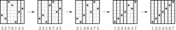
We use the following notation. Permutations will be written in one-line notation, . An ascent (resp. descent) is a gap between two neighbouring positions, and , such that (resp. ). Descents of split it into runs (maximal ascending strings), and ascents split it into falls (maximal descending strings). For example, the permutation splits into runs as , and into falls as .
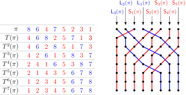
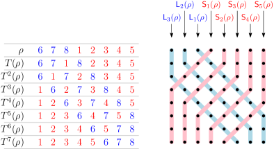
Flip-sort consists of iterating flips on the input permutation, where flip is the transformation that reverses all the falls of a permutation. For example, . If one applies repeatedly (thus obtaining ), then one eventually obtains the identity permutation . For example: ; see Figure 1 for a visualization of this example by means of permutation diagrams. Nota bene: if one does not impose the stack to contain increasing values, then the process can be related to the famous pancake sorting problem (see [20]).
Let the cost of be the (minimum) number of iterations needed to sort , that is, . To see that the cost is always finite, observe that at each iteration the number of inversions strictly decreases until is reached. It follows that, for any permutation of size , we have . In fact, the cost is always lower than this naive upper bound: Ungar [32] proved111This result was conjectured by Goodman and Pollack [21], and proved by Ungar, in the context of allowable sequences of permutations in links with the minimum number of directions determined by non-collinear points in the plane; see the crisp presentation of this nice geometrical question in [1, Chapter 12]. that one always has (we refine this result in our Section 4.2). Moreover, this bound is tight since for each there are permutations of size with cost (we give some examples in Section 4.4).
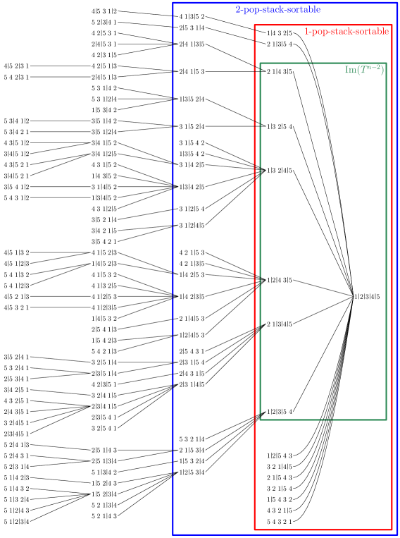
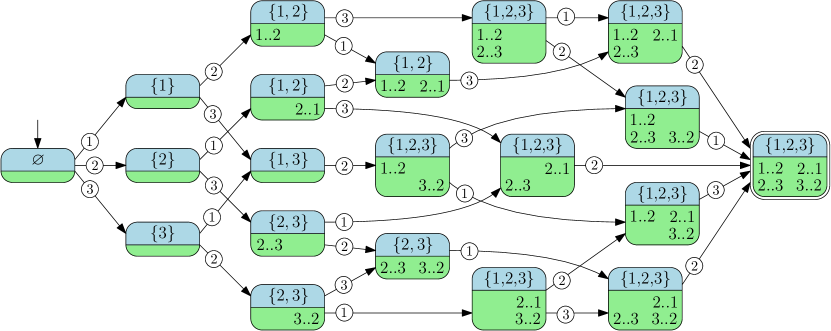
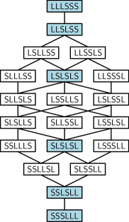
The pop-stack sorting leads to many interesting combinatorial questions. Some of them can be visualized by means of the pop-stack-sorting tree whose nodes are all permutations of size , with directed arcs from to . It is convenient to draw such a tree with levels corresponding to the distance to : see Figure 2 that shows the tree for (the arcs are understood to be directed from left to right). When, more generally, one considers this tree for any value of , it is natural to ask for a characterization of the permutations that need few iterations of to be sorted (i.e. the right side of the tree), or many iterations (i.e. the left side of the tree); or the image of (i.e. the non-leaves of the tree). We address these questions in this article, thus extending previous works [32, 28, 14].
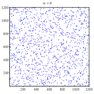
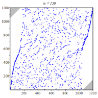
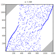
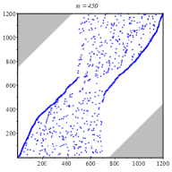
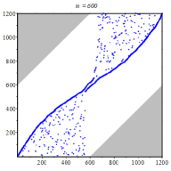
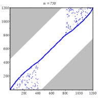
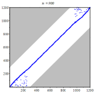
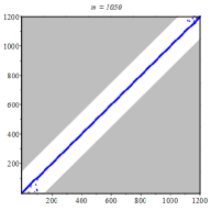
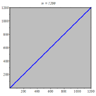
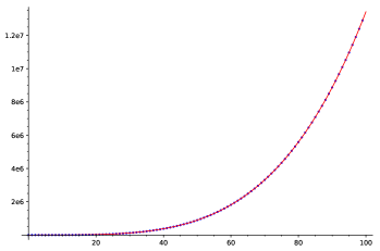
Another challenging problem is describing a typical shape of , as runs from to , for random . Computer simulations show a very distinctive shape of the corresponding permutation diagrams: they possess some empty areas and a cloud of points accumulating along two curves that tend to unite and ultimately converge to the identity permutation; see Figure 3. We prove a more rigorous formalization of some of these claims in this article.
1.2 Summary of our results
The article is organized as follows.
In Section 2, we study the permutations that belong to , the image of the flip transformation. We find a structural characterization of such permutations, and we prove that the generating function of these permutations is rational when the number of runs is fixed. We then use a generating tree approach to design some efficient algorithms enumerating such permutations. We also show that their generating function satisfies a curious functional equation, and we give an asymptotic bound.
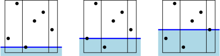
Section 3 is dedicated to permutations with low cost. A permutation is -pop-stack-sortable if , or, equivalently, . Avis and Newborn showed that -pop-stack-sortable are precisely the layered permutations [8], while -pop-stack-sortable permutations are recognizable by an automaton (see Claesson and Guðmundsson [14]). For , Pudwell and Smith [28] listed some conjectures that we prove via a bijection between -pop-stack-sortable permutations to a family of lattice paths.
In contrast, in Section 4, we deal with permutations with high cost, and with for arbitrary . Our main result is a (tight) bound on bandwidth of , which provides a partial explanation of the phenomena that we observe in Figure 3. Additionally, we find a full characterization of , and some conditions for . We conclude with a conjecture concerning the cost of skew-layered permutations.
 |
 |
 |
 |
 |
 |
 |
 |
 |
2 Results concerning one iteration of the flip-sort algorithm
2.1 Structural characterization of pop-stacked permutations
We start this section with a characterization of the image of , i.e. the internal nodes in the pop-stack tree from Figure 2.
Definition 1.
A permutation is pop-stacked if it belongs to , that is, if there is a permutation such that we have .
Definition 2.
A pair , of adjacent runs of is overlapping if . (Notice that holds automatically since and are distinct runs.)
We begin our investigations of the image of by giving a characterization of the permutations in in terms of overlapping runs. In fact, in the following theorem we prove that a permutation is pop-stacked if and only if all pairs of adjacent runs are overlapping. See Figure 4 for a schematic drawing that represents the structure of permutations with overlapping adjacent runs, and an example. Despite its very natural definition, this family of permutations was, to the best of our knowledge, never studied before our initial conference contributions [5, 4].

Theorem 3.
A permutation is pop-stacked if and only if all its pairs , of adjacent runs are overlapping.
Proof.
[First part of the proof: pop-stacked overlapping runs.] Let be a permutation with for some pair , of its adjacent runs. Let be the last letter in and be the first letter in (that is, , ).
Assume for contradiction that we have for some permutation . In , we have because otherwise the string is a part of a fall in , and upon applying we have , which is impossible, because and lie in different runs of . Therefore, if we consider the partition of into falls, then is the last letter of some fall , and is the first letter of the next fall . However, the values of are a subset of those of , and the values of are a subset of those of . Therefore we have , which is a contradiction to observed above.
[Second part of the proof: overlapping runs pop-stacked.] Consider a permutation with for all pairs , of adjacent runs. Let be the permutation obtained from by reversal of all its runs. Then the partition of into falls is the same as the partition of into runs, and, therefore, is a (not necessarily unique) pre-image of . ∎
2.2 Pop-stacked permutations with a fixed number of runs
Sections 2.2–2.4 are dedicated to enumerative aspects of pop-stacked permutations. Let denote the number of pop-stacked permutations of size . The sequence starts with 1, 1, 3, 11, 49, 263, 1653, 11877, 95991, 862047, 8516221, 91782159, 1071601285, 13473914281, 181517350571, 2608383775171, 39824825088809, 643813226048935; we have added it as A307030 to the On-Line Encyclopedia of Integer Sequences. While it is hard to compute more terms directly, the introduction of additional parameters provides further insights. Specifically, in this section we consider the number of runs in pop-stacked permutations. In particular, we show that for each fixed , the generating function for pop-stacked permutations of size with exactly runs is rational.
Let denote the number of pop-stacked permutations of size with exactly runs. The case is trivial: for any size, the only permutation with only one run is the identity permutation, and it is pop-stacked as it is e.g. the image of itself. Thus, we have for each . Note that, for , is always an even number (indeed, listing the runs from the last one to the first one gives an involution without fixed points among pop-stacked permutations), therefore is always an odd number.
One key ingredient of our further results is the following encoding of permutations, which we call scanline mapping. Let be a permutation with runs. Let be the index of the run in which the letter lies. Consider the word . Visually, we scan the graph of from the bottom to the top, and for each point that we encounter in this order, we record to which run it belongs; see Figure 5.
Proposition 4.
The scanline mapping has the following three properties.
-
1.
The scanline mapping is injective.
-
2.
The scanline mapping induces a bijection between permutations of size with runs and the words in in which there is an occurrence of before222N.B.: There should be some occurrence of somewhere before some occurrence of , not necessarily just before. For example, the sequence with satisfies the condition. Similarly for the last item of this proposition. an occurrence of , for each ().
-
3.
The scanline mapping induces a bijection between pop-stacked permutations of size with runs and the words in in which there is an occurrence of before an occurrence of , and also an occurrence of before an occurrence of , for each ().
Proof.
-
1.
The positions of () in are the values in the th run of . Thus, is reconstructed from uniquely.
-
2.
If (and only if) for some , all the occurrences of in are before the occurrences of , then the corresponding positions of do not form two distinct runs and thus we do not get a permutation with runs.
-
3.
If (and only if) for some , all the occurrences of in are before the occurrences of , then all the values in the th run of are larger than all the values in the st run, and thus these runs are not overlapping.
∎
Proposition 4 can be used to obtain a formula for the case of two runs directly:
Proposition 5.
For , the number of pop-stacked permutations of size with exactly two runs, is .
Proof.
By Proposition 4, is the number of words in with an occurrence of before an occurrence of , and also an occurrence of before an occurrence of . There are words that violate this condition (including the “all-1” and the “all-2” words). ∎
It is pleasant to have a combinatorial explanation for the number of pop-stacked permutations with two runs, and this game could be pursued (algorithmically) for a fixed number of runs , but to get a closed-form formula holding for any arbitrary number of runs is still open. While the following theorem does not give an explicit formula for all of those cases immediately, it proves that the counting sequence for pop-stacked permutations with precisely runs is nice and simple from a structural point of view.
Theorem 6.
Let be fixed. Then , the generating function for the number of pop-stacked permutations with exactly runs, is rational.
Proof.
It is well known that the generating function of words recognized by an automaton is rational (see e.g. [18, Sec. I.4.2]). We use Proposition 4 to construct a deterministic automaton over the alphabet that precisely recognizes the words that correspond to the pop-stacked permutations. The states of are labelled by pairs , where
-
•
indicates the already visited letters, and
-
•
indicates the already fulfilled conditions “there is an occurrence of before an occurrence of ” resp. “there is an occurrence of before an occurrence of ”, such that
-
•
if , then at least one of and belongs to .
It is then straightforward to see that precisely recognizes those words in that correspond bijectively to the pop-stacked permutations of size with runs by Proposition 4. Figure 6 shows such an automaton for . ∎
In the next theorem, we address the complexity of : its number of states grows roughly as . This exponential growth of the number of states also gives an insight on the complexity of the generating functions associated to these automata.
Theorem 7.
Denote by the number of states in the automaton . The sequence satisfies the linear recurrence . Together with initial conditions, this implies that is A006012: . Accordingly, the number of states of grows exponentially: .
Proof.
We proceed by induction on (starting at ). Denote by the set of states of the automaton defined in the proof of Theorem 6. Recall that the states are labelled by , where is the set of already encountered letters, and is the list of already fulfilled conditions of the kind or .
We partition the states of into three parts as follows.
-
1.
The states of whose letters do not contain : they are precisely all the states of .
-
2.
The states of whose letters contain but do not contain . They correspond bijectively to the states of whose letters do not contain , and thus to all the states of :
(1) where .
-
3.
Finally, the states of whose letters contain both and . They correspond -bijectively to the states of whose letters contain :
(2) where .
Therefore, summing over these three cases, we have
| (3) |
which completes the proof. ∎
Remark: Upon performing minimization on , we obtain automata with the number of states given by . This leads us to conjecture that this sequence satisfies the linear recurrence , and that it is in fact A293004333The goddess of combinatorics is thumbing her nose at us, as this sequence is also related to permutation patterns in many ways: it counts permutations related to the elevator problem [24, 5.4.8 Ex.8], permutations avoiding 2413, 3142, 2143, 3412, and some guillotine partitions [6]!. Possibly, this could be proved by following the impact of each step of Brzozowski’s algorithm for minimizing an automaton, see [13]. It is interesting to notice that the exponential growth of the number of states would then drop from to .
Before we continue with our investigations towards efficient computation of the numbers , we want to make some observations concerning the particular shape of the rational generating functions . Recall that Theorem 6 provides a construction for a deterministic finite automaton that recognizes pop-stacked permutations of length . Given such an automaton, the associated generating function can be extracted in a straightforward way. Doing so for yields the rational functions
Some further functions can still be computed in reasonable time. However, as the number of states in the automaton grows exponentially in , this approach is not feasible for large values of .
Note that the lowest degree in the numerator is . This is because the smallest possible permutation size for a pop-stacked permutation with runs can only be obtained by alternating runs of lengths 1 and 2. It is even possible to (experimentally) observe further structure in these , for example they have the following partial fraction decomposition:
| (4) |
where is a polynomial of degree in and in :
We listed the first few values of these polynomial in case that some clever mind could find the general pattern for any . We failed to find a generic closed-form formula, but it is noteworthy that the decomposition of Formula (4) has some similarities with the partial fraction decomposition of Eulerian numbers.
Proposition 8.
Consider the Eulerian numbers , defined as the number of permutations of size that have precisely runs444Sometimes, Eulerian numbers are defined such that enumerates all permutations of size that have descents. Both cases (counting with respect to runs vs. counting with respect to descents) can be obtained from each other by shifting by one.. The generating functions for the columns of the Eulerian number triangle have the following partial fraction decomposition
| (5) |
Proof.
We were surprised to find no trace of this nice formula in the literature, so we now give a short proof of it. First, inserting into a permutation of size with runs either enlarges one of the runs if is inserted at its end, or it creates a new run in all other cases; this gives the classical recurrence
| (6) |
From it, it is easy to get by induction that
We refer to [26, 19] for possible alternative proofs and thorough surveys on Eulerian numbers.
Then, rewriting the Eulerian numbers in by means of this formula and carrying out some algebraic manipulations yields
This proves the partial fraction decomposition.∎
The partial fraction decomposition (5) allows us to make statements about the structure of . We now list several of these properties, comparing them with our observations for the generating functions .
-
•
The degree of the numerator of is , and for we conjecture it to be .
-
•
The leading coefficient in the numerator of is (only the first summand in (5) contributes towards the maximum degree), and for we conjecture it to be .
-
•
For , summing the coefficients in the numerator yields (setting in the numerator of only collects contributions from the last summand in (5)), for we conjecture that it is .
While we think that it is unlikely that the sequence satisfies a simple linear recurrence relation as in (6), we derive in the next section a useful, but more complex, recurrence scheme that depends on some additional parameters.
2.3 A functional equation for pop-stacked permutations and the corresponding polynomial-time algorithm for the enumeration
As noted above, the counting sequence is hard to compute directly without introducing additional parameters. In [5], we mentioned that a generating tree approach leads to an efficient enumeration algorithm for pop-stacked permutations; it relies on an additional parameter which is either the number of runs, or the final value of the permutation. Such generating tree approaches lead to polynomial time algorithms for computing (see [9] for further examples of enumerations via generating tree approaches).
When the additional parameter is the number of runs, this gives a recurrence which encodes the addition of a new run of length to the end of a given permutation of size (and relabels this concatenation to get a permutation of size ). The cost of this approach is analysed in [15], and was implemented with care on a computer cluster, allowing the computation of the number of pop-stacked permutations of size , for all .
When the additional parameter is the final value of the permutation, this gives an approach that we now detail in this section. Based on a generation strategy where either one or two elements are added to a given permutation, we consider the corresponding generating tree. With this strategy, we can derive an appropriate recurrence which also allows us to compute the sequence in polynomial time, and also offers a functional equation for the corresponding multivariate generating function.
For this generation strategy, we need to keep track of a few additional parameters in pop-stacked permutations. Let , , , , be non-negative integers such that and . Let the set denote all pop-stacked permutations where
-
•
denotes the length of the permutation,
-
•
denotes the number of runs,
-
•
and denote the smallest and largest element of the last run, respectively,
-
•
if , then denotes the second-largest element of the last run; else, if , then also .
Just to give some examples, the permutation is contained in , is contained in , and .
The following set of rules describes how, starting from two initial permutation sets and , all other sets can be generated. This heavily relies on the characterization, given in Theorem 3, of pop-stacked permutations.
-
(Rule 1)
A new run consisting of a single element is added to the end of all generated permutations. For all integers with , this operation corresponds to an injection .
-
(Rule 2)
A new run consisting of two elements is added to the end of all generated permutations. For all integers with and , this corresponds to an injection .
-
(Rule 3)
Insert a new second-largest element into the last run of all generated permutations. For all integers with , this corresponds to the injection .
Proposition 9.
Proof.
In order to see that all permutations are generated by this strategy we study the corresponding inverse operation. Given a pop-stacked permutation of length that is different from or , we consider its last run. Then we carry out the following operations, based on the length of the final run:
- •
-
•
Otherwise, if the run is of length at least 3, the second-largest (and therefore penultimate) element is deleted. This is the reversal of 3.
After proper relabelling, this results in a shorter permutation that is still pop-stacked. Applying the appropriate expansion rule to constructs a set of “successors” also containing . Observe that by the nature of the expansion rules, only pop-stacked permutations can be generated (as long as we start with a pop-stacked permutation) as it is made sure that the last and the penultimate run always overlap.
This proves that for every permutation (apart from and ) a unique predecessor in the generating tree can be found. The permutations and are special in the sense that they are the only permutations for which the above strategy does not yield a well-defined result. At the same time, this implies that when starting at any other permutation and iterating the procedure of finding the predecessor eventually leads to either or . This proves that when starting with these permutations (in our notation, this corresponds to the sets and ), all other pop-stacked permutations can be generated by applying 1, 2, and 3 iteratively. ∎
Now, let us turn our focus from generating these permutations to their enumeration. Let , the number of pop-stacked permutations in . With the notation from Section 2.2, we have
The generating tree approach can be utilized to derive a functional equation for the associated multivariate generating function
| (7) |
as well as a recurrence scheme the numbers .
We begin with the functional equation for , which is proved by translating the expansion rules from above to the level of algebraic operations on generating functions.
Theorem 10.
The multivariate generating function as given in (7) satisfies the functional equation
| (8) | ||||
Proof.
This functional equation is just the reflection of the fact that any pop-stacked permutation is either empty, or one of the two roots of the generating tree, namely (encoded in (8) by the monomial ) or (encoded in (8) by ), or a permutation obtained by applying one the three expansions rules to a smaller pop-stacked permutation.
Now, each of the four remaining summands in the right-hand side of (8) can be explained by considering that each of the expansion rules acts as a linear operator on the monomials of the generating function . While the corresponding calculations are not too difficult, they can be a bit tedious — which is why we choose to illustrate it for one of the rules, and give only the results for the remaining ones.
Let us first consider 3, which describes the injection for . Starting from a given permutation whose associated monomial is , this rule generates longer permutations by inserting a new second-largest element into the last run. On the level of monomials, this corresponds to the map
As this operator is linear, its application to the generating function (seen as sum of monomials) leads to a sum which can itself also be written in terms of ; this yields a total contribution of
Similarly, 1 yields a total contribution corresponding to the summand
and 2 yields the two remaining summands on the right-hand side of (8). ∎
This allows us to obtain a recurrence relation for as given in the following theorem. Therein, for the sake of simplicity, we make use of the Iverson bracket , a notation popularized in [22], which evaluates to 1 if is a true expression, and 0 otherwise.
Theorem 11 (Polynomial-time computations for pop-stacked permutations).
Let , , , , be non-negative integers. The number of pop-stacked permutations of length with runs where the last run starts with , ends with , and where is either the penultimate element (if it exists) or coincides with and as given by satisfies the recurrence relation
| (9) | ||||
together with the initial conditions .
The number of pop-stacked permutations of length with runs is thus
| (10) |
and the number of pop-stacked permutations of length is thus , which can be computed with time-complexity and memory-complexity.
Proof.
We can either go back to the combinatorial description of the generation of permutations via the generating tree approach, or consider the functional equation (8) and extract the coefficient of the monomial on both sides in order to obtain the recurrence relation (9) for . Now, for the complexity analysis, observe that the triple sums appearing in the first and second branch of (9) can be computed more efficiently by defining the auxiliary sequence
and note that this sequence can be computed with a backward recurrence from to via
| (11) |
Furthermore, observe that we can actually rewrite the third branch of the recurrence (9) (for and ) as
We are now able to rewrite the recurrence in the form
| (12) | ||||
This approach allows us to compute for in arithmetic operations. Furthermore, observe that the number of runs is actually not relevant in the recurrence. If we were only interested in , the number of pop-stacked permutations of length , then we could drop this additional parameter: this allows us to compute for in arithmetic operations, with simultaneous allocations in memory. Actually, we can be even more precise and obtain the main asymptotic term of the number of operations: In the computation of for , the branches of the recurrence (12) are visited for all . Investigating these branches more closely reveals that while the case of is asymptotically negligible for the main term, both the case of as well as contribute to the total number of additions required. Finally, adding all for and , one gets more additions — which means that in total the number of additions behaves like . Similar considerations show that this approach requires simultaneous memory allocations. ∎
A straightforward implementation of the optimized recurrence (12) in SageMath [31] that stores relevant intermediate results in cache memory makes it possible to compute the first 100 terms of the sequence on a standard desktop PC in less than 3 minutes. Figure 7 illustrates the number of additions carried out by our strategy and confirms our assertion regarding the main asymptotic term.
However, unfortunately, neither the recurrence scheme nor the functional equation for the generating function yield sufficient leverage to carry out an exact analysis of the asymptotic behaviour of the sequence . In the following section, we provide a lower bound for the growth of and give pointers to experimental observations.
2.4 Asymptotics of pop-stacked permutations
In many cases, the growth of restricted families of permutations is much less than , and is just exponential: for example, by the Stanley–Wilf conjecture (proved by Marcus and Tardos [25]), this always holds for permutation classes defined by classical forbidden patterns. It is natural to ask whether this is the case for pop-stacked permutations. We now prove that they in fact grow much faster.
Theorem 12 (Superexponential growth of pop-stacked permutations).
The asymptotic growth of the number of pop-stacked permutations is at least .
Proof.
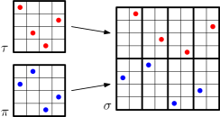
We achieve this by constructing an explicit class of permutations, as follows. Assume that is even, and consider any pair of permutations, and , each of size . Intertwine them as shown in Figure 8, i.e. consider the permutation of size defined by
| (13) |
It is easy to see that such is necessarily pop-stacked (it clearly satisfies the overlapping run condition from Theorem 3). Since the mapping is injective, we conclude that we have at least pop-stacked permutations of size . Then, Stirling’s approximation for the factorial leads to the theorem. Note that the fact that the above argument holds for even only is not a restriction: by inserting at the end of any pop-stacked permutation of length , one obtains a new pop-stacked permutation of size ; therefore the sequence is strictly increasing, and thus the Stirling bound given in the claim remains valid for odd . ∎
Due to the nature of the counting sequence and the fact that we have no appropriate representation of the associated generating function, an exact asymptotic analysis of the growth behaviour of the sequence remains a challenge. The above theorem gives a lower bound of , it is also possible to compare with André’s alternating permutations to get a lower bound of (see e.g. [18, p. 5]). Note that the authors of [15] carried out an experimental analysis using automated fitting and differential approximation. Their analysis of the counting sequence led them to conjecture that the corresponding exponential generating function possesses an infinite number of singularities, thus implying non-D-finiteness. Ultimately, they conjecture that the asymptotic growth of the sequence counting pop-stacked permutations of size is
see [15, Section 3.3] for more details.
3 Best cases of flip-sort: permutations with low cost
3.1 Notation and earlier work
Some of the earlier work on pop-stack sorting dealt with permutation with low cost. The following notation was introduced there.
Definition 13.
A permutation is -pop-stack-sortable if (or, equivalently, if ).
- and -pop-stack-sortable permutations are shown by the red and the blue frames in the pop-stack-sorting tree in Figure 2.
Several results concerning -pop-stack-sortability are known:
- •
-
•
Pudwell and Smith [28] found a structural characterization of -pop-stack-sortable permutations, as well as a bijection between such permutations and polyominoes on a twisted cylinder of width (see [3]). Moreover, they proved that the generating function for -pop-stack-sortable permutations is rational (we shall reprove their result below).
-
•
Claesson and Guðmundsson [14] generalized the latter result showing that for each fixed , the generating function for -pop-stack-sortable permutations is rational.
3.2 The pre-images of -pop-stack-sortable permutations
We begin with a nice enumerative result in which the notion of - and -pop-stack-sortable permutations is combined with our notion of pop-stacked permutations. Specifically, it concerns those -pop-stack-sortable permutations that belong to the image of (thus, corresponding to internal nodes in the right column before the identity in the pop-stack tree from Figure 2).
Theorem 14.
Pop-stack layered permutations have the following properties:
-
1.
Let be the set of pop-stacked layered permutations (or, equivalently, of -pop-stack-sortable permutations that belong to ) of size . The generating function for is
(14) Consequently, this family is enumerated by “tribonacci numbers” (A000213).
-
2.
Let . All the permutations such that can be constructed by the following procedure:
-
•
Put primary bars at all descents of .
-
•
Optionally, put secondary bars at some descents so that each primary bar has at least one neighbouring position without any bar.
-
•
Reverse all the blocks determined by the bars.
-
•
Proof.
-
1.
Let be a layered permutation of size . Partition it into falls. Refer to the first and the last falls as outer falls, to all other falls as inner falls. For it is easy to see that we have non-overlapping adjacent runs if and only if there is an outer fall of size or an inner fall of size . For the permutation is pop-stacked, and the permutation is not. It follows that for we have if and only if it has at least two falls, the outer falls being of size or , the inner falls of size or or . This implies the generating function (14).
-
2.
As is obtained from by reversing all its falls, is obtained from by reversing its runs — possibly, further partitioned. That is, we must first partition into runs (by primary bars), then optionally further partition the runs (by secondary bars), then reverse all the blocks.
We need to prove the condition on secondary bars. Suppose a primary bar separates a descent (we have ). If we put bars at both adjacent gaps, , then we have the same values in positions and in . However, this would be a descent, that is, a part of a fall in , and it should be reversed when we apply . Otherwise, both sub-runs (that from the left and that from the right of the primary bar) will yield, upon reversal, two distinct falls in , that will recover these sub-runs when we apply .
∎
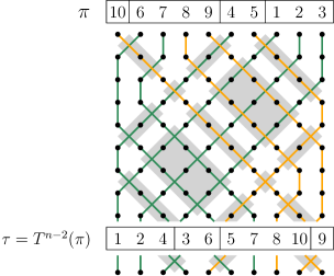
Example. Let . The primary bars are inserted at the descents: . All the possibilities to insert secondary bars (for the sake of clarity, we indicate them by ) are , , , , , which gives all the pre-images of : , , , , . Further, it can be shown that the number of pre-images of is always the product of some Fibonacci numbers depending on the sequence of sizes of falls of .
3.3 -pop-stack-sortable permutations and lattice paths
In this section we extend some of the results by Pudwell and Smith [28]. Namely, we reprove one of their theorems and prove (a generalization of) one of their conjectures. All this is done via the uniform framework of lattice paths. By doing this, we not only construct a bijection between -pop-stack sortable permutations and lattice paths, but also benefit from the fact that the theory of lattice paths is well developed (see e.g. [10]), thus offering additional structural insight.
First, we reprove the theorem by Pudwell and Smith in a more combinatorial way. Then we construct a bijection between -pop-stack-sortable permutations and a certain family of lattice paths, which enables us to prove two of their conjectures.
Theorem 15.
For , , let be the number of -pop-stack-sortable permutations of size with exactly ascents.
The two-dimensional array is shown in Figure 9. The th row () contains coefficients . The “diagonal-parallel” arrays from part 2 are vertical in this drawing ( corresponds to , to , etc.).

Proof.
-
1.
It is shown in [28, Lemma 2.1] that a permutation is -pop-stack-sortable if and only if for each pair of its adjacent falls, and , one has .666Notice that layered permutations are similarly characterized by . Consider an ascent that separates two adjacent falls and . We say that this ascent is regular if , and twisted if . An ascent can be twisted only when at least one of the falls or is of size (equivalently, when at least one of the adjacent gaps is a descent).
As Pudwell and Smith show, -pop-stack-sortable permutations are bijectively encoded by sequences of their ascents and descents (we use for ascents, for descents), where for each that has an adjacent it is indicated whether this is regular or twisted. We find it convenient to use instead lattice paths: we replace each by the up-step , by the down-step , and corner-adjacent -steps (that is, -steps which have at least one adjacent -step) will be bicoloured: -steps that correspond to a regular ascent will be coloured black, -steps that correspond to a twisted ascent will be coloured red. In this way, we obtain a certain family of Dyck walks. The length of a walk is smaller by than the size of the corresponding permutation, and the final altitude is . See Figure 10 for illustration.
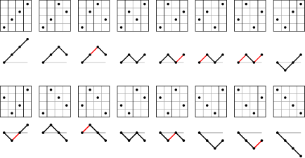
Figure 10: Encoding of -pop-stack-sortable permutations by Dyck walks with bicoloured corner-adjacent -steps. To enumerate such walks, we make use of the symbolic method (see [18, Chapter I]) to find a combinatorial specification for (non-coloured) Dyck walks in which corner-adjacent -steps are marked by :
This leads to the following functional equation for the trivariate generating function , where is the variable for length, for final altitude, for occurrences of corner-adjacent -steps:
(18) This yields the generating function
(19) and the bivariate generating function for those walks in which corner-adjacent -steps are bicoloured, is
(20) Upon performing the transformation that corresponds to the way in which we rearranged the array of the coefficients, we obtain . This completes the proof of part 1.
-
2.
First, we find the generating function for excursions — that is, those walks that stay (weakly) above and terminate at the -axis — in our model of Dyck walks with marked corner-adjacent -steps. The functional equation for is
(21) which yields
(22) Therefore, the generating function for Dyck excursions with bicoloured corner-adjacent -steps is
(23) (In fact, we have , where is the generating function for Motzkin numbers. This can be shown bijectively, starting from the fact that the number of Dyck excursions of semilength with exactly corner-adjacent -steps, is , where is the st Motzkin number. A similar result on Dyck paths with marked pattern was proved by Sun in [30, Thm. 2.2].)
The “diagonal coefficients” of correspond to coefficients of . Therefore we look for the generating function for bridges — that is, those walks that terminate at the -axis — in our model. It can be routinely found by residue analysis (extracting in ). However, we give a more structural proof. We decompose a bridge into an alternating sequence of excursions and anti-excursions ( rotated by excursions that stay weakly below the -axis). Since we use only and steps, such a decomposition is unambiguous. Moreover, the generating function for anti-excursions is the same as for excursions. When we join excursions and anti-excursions, new corner-adjacent -steps are never created. Therefore we have
(24) and finally
(25) Notice that we can rewrite this as
and the coefficients of are well known to be central binomial coefficients. This directly leads to the first closed-form formula of Equation (17) for . The second equivalent closed-form formula is proved easily via closure properties from holonomy theory; see [27].
Finally, we consider generating functions for walks that terminate at fixed altitude . For unmarked paths we have the classical decomposition . Taking care of corner-adjacent -steps, we obtain, for ,
and
which, upon due modification, yields (16).
∎
Finally, if we look again at (20) and rewrite it in the form then it is immediate from the theory of lattice paths that it is also the bivariate generating function for lattice paths that start either at or at , and use steps , , , and bicoloured .
![[Uncaptioned image]](/html/2003.04912/assets/x19.png)
These paths can also be used to obtain formulas (16) for diagonal-parallel arrays, and the computations are even easier because the bicolouration of some steps does not require considering their adjacent steps.
![[Uncaptioned image]](/html/2003.04912/assets/x20.png)
4 Worst-cases of flip-sort: permutations with high cost
“Conventional wisdom might say that extremal problems tend to be very difficult to solve exactly if the extreme configurations are so diverse and irregular.”
Martin Aigner & Günter Ziegler, in Proofs from THE BOOK.
This claim by Aigner and Ziegler is concerning an extremal problem in geometry which is in fact solved by understanding the worst cases of flip-sort! We refer to [1, Chapter 12] and [32] for more details on this geometric problem. In this section, we strongly extend these studies by proving structural and enumerative results concerning the evolution of permutations during the flip-sort process, focussing on permutations with worst costs. We start with some definitions, notation, and basic observations.
4.1 Definitions and notation
By we denote the identity permutation of size , and by we denote its reversal: , and .
Definition 16 (Layered and skew-layered permutations).
The layered permutation is the direct sum of . The skew-layered permutation is the skew sum of .777We refer to Permutation patterns: basic definitions and notation by David Bevan [11] for the definitions of direct sum and of skew sum. For example, and .
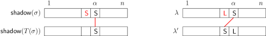
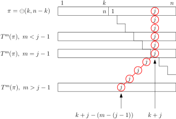
Definition 17 (-shadows).
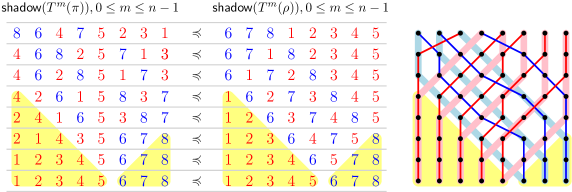
Let be a permutation of size , and let be a fixed number, . Let , ( for small, for large). The -shadow of is defined to be the -word obtained from by replacing all the numbers from by , and all the numbers from by . When is fixed, we shall usually omit the subscript and write just . Example: for we have .
For , we denote by the position of the th occurrence of counted from left in ; for , we denote by the position of the th occurrence of counted from right in . In the example just considered, we have , , ; , , , .
Definition 18 (- and -paths, -wiring diagram).
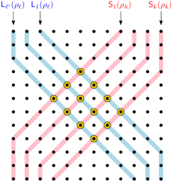
Let and be as above. For , the th -path is the sequence . For , the th -path is the sequence . The -wiring diagram is a drawing on the rectangular grid with infinitely many rows, labelled (from above) by , that correspond to ; and columns labelled by . In this drawing, we represent the th -path () by a polygonal red line connecting the points , and we represent the th -path () by a polygonal blue line connecting the points . The th -path (resp. -path) of will be denoted by (resp. by . See Figure 11 for an example.
Remark: Since we show below that after the st row the paths stay in the same position (namely, the in the position , and the -path in the position ), we draw -wiring diagrams with only rows, from the one corresponding to to the one corresponding to .
In the following considerations, the -wiring diagram of the permutation will play an important role. When is fixed, we shall usually omit the subscript and write just . It is easy to verify that , and that for each the word is obtained from by replacing each consecutive occurrence of by . This yields
|
|
(26) |
Accordingly, the -wiring diagram of has a very distinctive shape, with - and -paths typically consisting of three segments. This is illustrated in Figure 12 (since we later combine the -wiring diagram of the fixed permutation with that of an arbitrary permutation , the - and -paths of will be shown by thick pink and light-blue lines). Finally, we notice that, since the sets and are already sorted in , all the values along are , and all the values along are , so that for the -wiring diagram coincides with the usual wiring diagram where paths connect occurrences of the same value.
Definition 19 (Poset of words).
Assume . Let be the set of words of length with occurrences of and occurrences of . For we write if for each , , the position of the th in is weakly to the left from the position of the th in . Equivalently, if for each , , the position of the th in is weakly to the right from the position of the th in 888We remind that the occurrences of are counted from left, and the occurrences of are counted from right.. For example, . It is easy to verify that is a partial order relation, and that these two definitions are indeed equivalent.
In fact, is the transitive closure of the relation “ is obtained from by replacing some consecutive occurrence of by ”. In particular, it follows that — the maximum element of — covers just one element: , and that — the minimum element of — is covered by just one element: .
See Figure 13 for the Hasse diagram of with the partial order , for (the words marked by blue colour are the -shadows of ).
Definition 20 (Bandwidth).
The bandwidth (also called maximum displacement) of a permutation is
| (27) |
The inequality corresponds to the diagram of being -diagonal. This means that it is entirely contained in the main diagonal and its shifts to either side. Obviously, for each permutation of size , we have , and if and only if .
4.2 The worst case: iterations, and a key statistic: bandwidth of permutations
The main result of this section is the following theorem about the bandwidth of a permutation in . In terms of permutation diagrams, this theorem says that grey areas as in Figure 3 do not contain any points of respective diagrams.
Theorem 21.
If (where ), then we have .
Notice that for we obtain that a permutation in has , and thus we recover Ungar’s result mentioned above, . The proof that we give is also a generalization of Ungar’s proof of this special case999Note that another perspective on Ungar’s result can also be found in the recent work of Albert and Vatter [2], inspired by Knuth’s zero-one principle [24, Theorem Z of Section 5.3.4], and offering links with a nondeterministic sort..
The proof of Theorem 21 will follow from the following propositions.
Proposition 22.
Let be a permutation of size . Let . Let (the poset defined in Definition 19) such that . Let be the word obtained from by replacing each consecutive occurrence of by . Then we have: If then .
Proof.
The word is obtained from by flips of the form (for some ), induced by flips in . It follows that for each () we have . Moreover, if and the st position in is , then we have . As for : since all the flips in are of the form , we always have or .
In terms of -wiring diagram, this means that -paths are monotone in the sense that, as we scan them from the top to the bottom, they move weakly to the left at each step. Moreover, if there is before , then the path that goes through this will move strongly to the left at the next step.
We now prove the claim. Assume for contradiction that we have but . Due to the properties just seen, this can only happen if for some , we have (see Figure 14). Since , the st position in is occupied by . Since , the st position in is occupied by . This means and , which contradicts .
∎
The next proposition is a rephrasing of one of the claims in Ungar’s proof.
Proposition 23.
Let be any permutation of size , and let . Let as defined in Section 4.1. Then, for each (), we have for -shadows .
Proof.
First, we have because in the letters occupy the last positions.
Then, the claim follows from Proposition 22 by induction since for we have . ∎
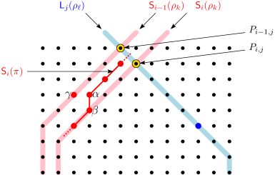
In terms of -wiring diagrams, Proposition 23 says that the paths in the -wiring diagram of majorize the paths in the -wiring diagram of in the following sense: for each (), the path is weakly to the left of the path ; and similarly, for each (), the path is weakly to the right of the path . For illustration, see Figure 15 in which - and -paths of (thin red and blue lines) are shown together with - and -paths of (thick pink and light-blue lines).
We now can complete the proof of Theorem 21 on the bandwidth of permutations in .
of Theorem 21.
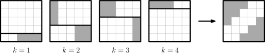
We notice that, along the last (vertical) segment of any path of , the corresponding path of coincides with it (these areas are marked by yellow triangles in Figure 15). More formally, it follows from Proposition 23 and from Equations (26) (which describe the shape of the - and -paths of ) that
| (28) | |||
| (29) |
In terms of permutation diagrams, Equations (30) and (31) (for fixed ) mean that for each some rectangular areas in the diagram of are forbidden. Taking the union of these areas for , we obtain forbidden corners, which yield the bound on the bandwidth. See Figure 16 for illustration (the forbidden areas are indicated by grey colour).
In Figure 17 we show the forbidden corners for and .
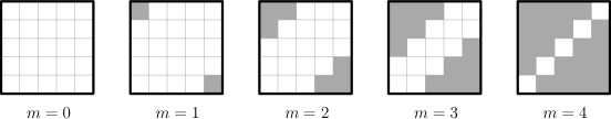
Now, if we compare this to Figure 3 (where grey areas are precisely those forbidden by Theorem 21), we see many other areas without points, and it is natural to ask whether there are some larger forbidden areas. In fact, contrary to what Figure 3 could suggest, the forbidden areas characterized in Theorem 21 are maximal in the sense that for each position outside the grey corners we can find a permutation that contains a point at this position. In fact, all the positions not forbidden by Theorem 21 are “covered” by skew-layered permutations with runs, as our next result shows.
Proposition 24.
Let be fixed, and let . For , let . Then there exists , a skew-layered permutation with runs, such that for we have .
Proof.
Assume . Let where will be determined below. From (26) and discussion thereafter, we know: if then for , if then for , and if then . Solving the first two expressions for we obtain that we need to set if , and if .
The case is similar, and for we can take which will do for any . ∎
Finally, we remark that, since Theorem 21 establishes that the bandwidth of allowed positions for permutations in decreases with , one can be tempted to conjecture that for we always have . Such a claim would, of course, imply Theorem 21! However, such a conjecture is wrong: the smallest counter-example is , and it is easy to see that any skew-layered permutation with at least two blocks, such that the first and last blocks are of size , is a counter-example.
4.3 The penultimate step of flip-sort: the theorem about .
In view of Ungar’s result, we have . The main result of this section is a structural characterization of . According to Theorem 21, implies . In fact, is a necessary, but not sufficient, condition for being in . (For example, for , one can see in Figure 2 that the permutation with is not in .) However, permutations that satisfy with will play an important role in our next results, and so we introduce a notation for them, and list some of their (nearly obvious) properties.
Definition 25.
A permutation is thin if .
Observation 26.
-
1.
A thin permutation is uniquely defined by the sequence of lengths of its runs. The thin permutation with runs of lengths (left to right) will be denoted by . For example, . If , the runs with will be referred to as inner runs.
-
2.
A sequence of natural numbers is realizable as the sequence of lengths of runs of a thin permutation if and only if for .
-
3.
Any inner run of a thin permutation has the form
The first and, respectively, the last run, have the forms
-
4.
A thin permutation is also uniquely defined by the sequence of lengths of its falls, that can only have lengths or . Any -sequence is realizable as the sequence of lengths of falls of a thin permutation. It follows that thin permutations are enumerated by Fibonacci numbers.
Now we state and prove the characterization of .
Theorem 27.
A permutation belongs to if and only if it is thin and has no inner runs of odd size.
Accordingly, for even , for odd (OEIS A052955)101010OEIS stands for the On-Line Encyclopedia of Integer Sequences, accessible at https://oeis.org/..
Proof.
[First part of the proof: is thin and with no inner runs of odd size.] Let . By Theorem 21 we have : thus, is thin. The second condition will be proved by contradiction. To this end we assume that is a thin permutation with at least one inner run of odd size, and that we have for some permutation . Specifically, we assume that has a run such that , , is odd, and (because, by Observation 26.2, a thin permutation has no inner runs of size ).
For the proof, we shall exploit shadows and wiring diagrams for both and . First, due to Observation 26.3, we know the - and the -shadows of :
| (32) |
Now we introduce the -wiring diagram of : the drawing that consists of -paths from the -wiring diagram of , and the -paths from the -wiring diagram of . Thus, in the -wiring diagram we have (red) -paths: for , the th -path (denoted by ) connects the th from left occurrences of the values from ; and we have (blue) -paths: for the th -path (denoted by ) connects the th from right occurrences of the values from . The remaining values from are not connected by paths in such a diagram.
Additionally, we consider the pink paths of and the light-blue paths of . By Proposition 23, these paths majorize the corresponding paths of : For , the path is weakly to the left from the , and for , the path is weakly to the right from the .
At this point we notice that, since is odd, all the pink paths and the light-blue paths cross each other at grid points of the diagram, see Figure 19. (Compare with Figure 12, where pink and light-blue paths cross each other between the rows of the diagram!) Denote by (, ) the crossing point of the path and the path : we refer to these points as conflict points.
Since , it is impossible that both and pass through . This means that in the row of , at least one of the paths and is strongly majorized by the corresponding pink or, respectively, light-blue path.
For we say that the pair is regular if some point of lies on after and before and reach their final position , and some point of lies on after and before and reach their final position . Next we prove two claims:
-
•
Claim 1: The pair is regular.
Indeed, we have and ; this means that, in the row which corresponds to , coincides with , and coincides with . In both cases, the paths are after the conflict points and before their final columns. -
•
Claim 2: If a pair is regular, then at least one of the pairs , is regular.
At least one of the paths , does not contain the point . Assume without loss of generality that does not contain the point . That is, in the row of , is strictly to the left from the pink path . Since has later a point that lies on (after , but before both paths reach their final position ), it makes a vertical step there, from a point to a point (refer to Figure 20). But this means that , the left neighbour of , is also from . Therefore is a point of on , after but before both paths reach their final position . This means that the pair is regular. (If we assume above that does not contain the point , we obtain that is regular.)
Starting with Claim and applying Claim repeatedly, we obtain that the pair is regular. However, the proof of Claim applies to as well. Since is the highest conflict point, we get a contradiction.
It is also possible to reverse this proof and to explain it “from the top to the bottom”. Then it essentially says that at least one of the sets, and , arrives at its final position sooner than in iterations. However in these sets are not at their final position (as witnessed by (32)), and this is a contradiction.
[Second part of the proof:
is thin and with no inner runs of odd size .]
For each which is a thin permutation without odd inner runs,
we will construct such that .
If we can take , so we assume from now on that .
Let so that and the numbers are even.
We define to be the skew-layered permutation .
We claim that for this we have . To see that, we analyse the wiring diagram of ; an example is illustrated in Figure 21. Notice that this is the usual wiring diagram, in which paths connect fixed values. For the sake of visualization, each inner run of is partitioned into two blocks of equal size, the left one and the right one. For the values from the left blocks of inner runs, and for all the values from the last run, we colour the paths in green. For the values from the right blocks of inner runs, and for all the values from the first run, we colour the paths in orange. Then, the paths have very clear description. Specifically, for an inner run of length , the th from left value () generates the green path that consists of segments (some of them can be empty): (1) a vertical segment of length , (2) a slanted segment of slope until the path reaches the position , (3) a vertical segment of length , (4) a slanted segment of slope until the path reaches its final position, (5) a vertical segment. The green paths of the last run do not have (4) and (5); orange paths are described similarly. The whole diagram is symmetric, and therefore the sequence of lengths of runs of is the reversal of the sequence of lengths of runs of .
Our proof shows that in order to construct a permutation in , one only has to choose positions (of the same parity) for the gaps between runs. This yields the enumerative formula, as stated in the claim. ∎
Remark. In general, there are several permutations that satisfy for given . Characterizing all such is a challenging problem.
4.4 Skew-layered permutations: a family of worst cases
By Theorem 27, each skew-layered permutation of size without odd inner runs has the (maximum possible for permutations of size ) cost . Characterizing all permutations with that cost is a challenging open problem. In this section, we present a necessary condition, and then we conclude with a conjecture concerning the cost of any skew-layered permutation.
Proposition 28.
Let be a permutation of size with . Let .
-
1.
There exists , , such that .
-
2.
For each such , we have . Consequently, can be written as a skew sum , where are permutations of sizes .
Proof.
-
1.
Since , we have . For each with we can take , and for each with we can take .
-
2.
In order to find a contradiction, assume that . Since the only element of the set of words covered by is , we necessarily have . Then, by Proposition 22 and by induction, we have , that is, , which is a contradiction. ∎
As for skew-layered permutations, we expect that their cost is always high (excluding the cases of and ); however, this cost is not always . Our computer experiments then suggest the following classification.
Conjecture 29.
Let be a skew-layered permutation of size such that is neither nor .
-
•
For even , one has .
-
•
For odd , if the -st position of is the central point of a run or of a fall of size , then . Otherwise, .
As a direct corollary of this conjecture, among the skew-layered permutations, there are:
-
•
for even , skew-layered permutations with ;
-
•
for odd , skew-layered permutations with ,
-
•
for odd , skew-layered permutations with .
These are respectively the sequences A000918, A020988, and A080675 from the OEIS.
5 Conclusion
In this article, we have seen that a simple sorting procedure like flip-sort has many interesting combinatorial and algorithmic facets. Our analysis of the best cases and the worst cases of this algorithm, our results on the underlying poset, the links with lattice paths, are just some first steps towards a more refined understanding of this process.
En passant, we listed a few conjectures, which, we hope, could tease the desire of the reader to work on this topic. The optimal cost of the computation of pop-stacked permutations is still open; other challenges are a finer analysis of the automata which recognize them (when the number of runs is fixed), the existence of closed-form formulas, a method to solve puzzling functional equations like the one given in Theorem 10.
We also believe that several of the notions and structures introduced in this article can also be useful for the next natural step: the average-case analysis of flip-sort. Even if this algorithm is not, in its naive version, as efficient as quicksort, it is very easy to implement, to parallelize, and it is still possible to optimize its implementation (this is a subject per se, like using double chained lists to perform the flips efficiently, or using some additional data structures to have a parsimonious reading of each iteration, etc). So there is not a “flip-sort” algorithm, but a family of flip-sort algorithms, and to finely tune them in order to decide what could be the optimal variant should clearly be the subject of future research.
Acknowledgements.
This research was supported by the Austrian Science Fund (FWF) in the framework of the project Analytic Combinatorics: Digits, Automata and Trees (P 28466). Cyril Banderier thanks the Department of Mathematics at the University of Klagenfurt for funding his visit in July 2019. Let us end by thanking the referees for their feedback.References
- [1] Martin Aigner and Günter M. Ziegler. Proofs from THE BOOK. Springer, 2018. Revised and enlarged 6th edition (1st ed: 1998).
- [2] Michael Albert and Vincent Vatter. How many pop-stacks does it take to sort a permutation? Computer Journal, to appear.
- [3] Gadi Aleksandrowicz, Andrei Asinowski, and Gill Barequet. Permutations with forbidden patterns and polyominoes on a twisted cylinder of width 3. Discrete Mathematics, 313(10):1078–1086, 2013.
- [4] Andrei Asinowski, Cyril Banderier, Sara Billey, Benjamin Hackl, and Svante Linusson. Pop-stack sorting and its image: permutations with overlapping runs. Acta Mathematica Universitatis Comenianae. New Series, 88(3):395–402, 2019. Proceedings of the European Conference on Combinatorics, Graph Theory and Applications (EuroComb 2019, Bratislava, 26-30 August 2019).
- [5] Andrei Asinowski, Cyril Banderier, and Benjamin Hackl. On extremal cases of pop-stack sorting. In Proceedings of Permutation Patterns 2019 (Zürich, 17-21 June 2019), 2019.
- [6] Andrei Asinowski and Toufik Mansour. Separable -permutations and guillotine partitions. Annals of Combinatorics, 14(1):17–43, 2010. [doi].
- [7] Michael D. Atkinson and Jörg-Rüdiger Sack. Pop-stacks in parallel. Information Processing Letters, 70(2):63–67, 1999. [doi].
- [8] David Avis and Monroe Newborn. On pop-stacks in series. Utilitas Mathematica, 19:129–140, 1981.
- [9] Cyril Banderier, Mireille Bousquet-Mélou, Alain Denise, Philippe Flajolet, Danièle Gardy, and Dominique Gouyou-Beauchamps. Generating functions for generating trees. Discrete Mathematics, 246(1-3):29–55, 2002.
- [10] Cyril Banderier and Philippe Flajolet. Basic analytic combinatorics of directed lattice paths. Theoretical Computer Science, 281(1-2):37–80, 2002.
- [11] David Bevan. Permutation patterns: basic definitions and notation. arXiv, 2015.
- [12] Miklós Bóna. Combinatorics of Permutations. CRC Press, 2012. Second edition (1st ed: 2004).
- [13] Janusz A. Brzozowski. Canonical regular expressions and minimal state graphs for definite events. In Proceedings of the Symposium on Mathematical Theory of Automata (New York, 24-26 April 1962), pages 529–561. Polytechnic Press, Brooklyn, 1963.
- [14] Anders Claesson and Bjarki Ágúst Guðmundsson. Enumerating permutations sortable by passes through a pop-stack. Advances in Applied Mathematics, 108:79–96, 2019. [doi].
- [15] Anders Claesson, Bjarki Ágúst Guðmundsson, and Jay Pantone. Counting pop-stacked permutations in polynomial time. Experimental Mathematics, To appear.
- [16] Colin Defant. Counting 3-stack-sortable permutations. Journal of Combinatorial Theory, Series A, 172:105–209, 2020. [doi].
- [17] Serge Dulucq, Sophie Gire, and Olivier Guibert. A combinatorial proof of J. West’s conjecture. Discrete Mathematics, 187(1-3):71–96, 1998.
- [18] Philippe Flajolet and Robert Sedgewick. Analytic Combinatorics. Cambridge University Press, 2009.
- [19] Dominique Foata and Marcel-Paul Schützenberger. Théorie géométrique des polynômes eulériens. Lecture Notes in Mathematics, Vol. 138. Springer, 1970.
- [20] William H. Gates and Christos H. Papadimitriou. Bounds for sorting by prefix reversal. Discrete Mathematics, 27(1):47–57, 1979.
- [21] Jacob E. Goodman and Richard Pollack. A combinatorial perspective on some problems in geometry. Congressus Numerantium, 32:383–394, 1981. Proceedings of the 12th Southeastern Conference on Combinatorics, Graph Theory, and Computing (Baton Rouge, 2–5 March 1981).
- [22] Ronald L. Graham, Donald E. Knuth, and Oren Patashnik. Concrete Mathematics. A Foundation for Computer Science. Addison-Wesley, 1994. Second edition (1st ed: 1988).
- [23] Donald E. Knuth. The Art of Computer Programming. Vol. 1: Fundamental Algorithms. Addison-Wesley, 1998. Third edition (1st ed: 1968).
- [24] Donald E. Knuth. The Art of Computer Programming. Vol. 3: Sorting and Searching. Addison-Wesley, 1998. Second edition (1st ed: 1973).
- [25] Adam Marcus and Gábor Tardos. Excluded permutation matrices and the Stanley–Wilf conjecture. Journal of Combinatorial Theory, Series A, 107(1):153–160, 2004.
- [26] T. Kyle Petersen. Eulerian numbers. Birkhäuser/Springer, 2015.
- [27] Marko Petkovšek, Herbert S. Wilf, and Doron Zeilberger. . A. K. Peters, 1996.
- [28] Lara Pudwell and Rebecca Smith. Two-stack-sorting with pop stacks. Australasian Journal of Combinatorics, 74(1):179–195, 2019.
- [29] Robert Sedgewick. Algorithms in C. Parts 1-4: Fundamentals, data structures, sorting, searching. Addison-Wesley, 3rd edition, 1997.
- [30] Yidong Sun. The statistic “number of udu’s” in Dyck paths. Discrete Mathematics, 287(1-3):177–186, 2004.
- [31] The Sage Developers. SageMath, the Sage Mathematics Software System (Version 9.2), 2020. http://www.sagemath.org.
- [32] Peter Ungar. noncollinear points determine at least directions. Journal of Combinatorial Theory. Series A, 33(3):343–347, 1982.
- [33] Julian West. Sorting twice through a stack. Theoretical Computer Science, 117(1-2):303–313, 1993. Conference on Formal Power Series and Algebraic Combinatorics (Bordeaux, 1991).