Disorder-free localization in an interacting two-dimensional lattice gauge theory

Abstract

Disorder-free localization has been recently introduced as a mechanism for ergodicity breaking in low-dimensional homogeneous lattice gauge theories caused by local constraints imposed by gauge invariance. We show that also genuinely interacting systems in two spatial dimensions can become nonergodic as a consequence of this mechanism. Specifically, we prove nonergodic behavior in the quantum link model by obtaining a rigorous bound on the localization-delocalization transition through a classical correlated percolation problem implying a fragmentation of Hilbert space on the nonergodic side of the transition. We study the quantum dynamics in this system by means of an efficient and perturbatively controlled representation of the wavefunction in terms of a variational network of classical spins akin to artificial neural networks. We identify a distinguishing dynamical signature by studying the propagation of line defects, yielding different light cone structures in the localized and ergodic phases, respectively. The methods we introduce in this work can be applied to any lattice gauge theory with finite-dimensional local Hilbert spaces irrespective of spatial dimensionality.

Introduction. Systems with local constraints play an important role in various physical contexts ranging from strongly correlated electrons Rokhsar:1988 and frustrated magnets Gingras:2014 ; Stern:2019 to fundamental theories of matter such as quantum electro- and chromodynamics Rothe:book , where constraints take the form of local gauge symmetries. The equilibrium properties of such systems have been extensively studied over the last decades, but only recently their nonequilibrium dynamics has moved into focus. In particular, local constraints have emerged as a new paradigm for ergodicity breaking, besides the two known archetypical scenarios caused by localization due to strong disorder or integrability. Systems with local constraints can exhibit rare nonergodic eigenstates, termed quantum many-body scars Turner:2018 ; Motrunich:2019 , or extremely slow relaxation Horrsen:2015 ; Pancotti:2019 ; Lan:2018 , whereas dipole conservation can prevent thermalization of large parts of the spectrum in one-dimensional fractonic systems Sala:2019 ; Pai:2019-PRL ; Pai:2019-PRX ; Khemani:2019 . A particularly generic mechanism for nonergodic behavior is hosted in lattice gauge theories (LGTs) where local constraints emerge naturally due to the local gauge symmetry, leading to an extensive number of local conserved quantities. Specifically, this can lead to the absence of ergodicity in 1D LGTs with discrete Smith:2017a ; Smith:2017b and continuous Brenes:2018 gauge symmetries or for higher-dimensional systems in the low-energy limit Haah:2016 or when they are free Smith:2018 . It has remained, however, a key challenge to rigorously identify non-ergodic behavior in genuinely interacting quantum matter beyond one dimension.

In this work we show that the 2D $U(1)$ quantum link model features both localized and ergodic phases in the absence of disorder. Our proof relies on a mapping onto a classical correlated percolation problem providing a rigorous bound on the localization transition of the quantum model. We identify a distinguishing quantum-dynamical signature of the two phases by studying the propagation of an initial line defect, which leads to two different light cone structures. For the description of the nonequilibrium dynamics of the system we introduce variational classical networks (vCNs), which provide an efficient and perturbatively controlled representation of the quantum many-body wave function in terms of a network of classical spins akin to artificial neural networks (ANNs). The introduced methods can be applied to any LGT with finite local Hilbert spaces irrespective of dimensionality.

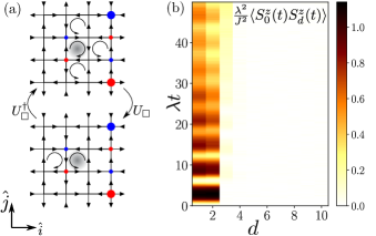
Figure 1: a) Illustration of the $U(1)$ quantum link model (QLM) with spin-1/2’s located on the links of the square lattice. Spins pointing $\rightarrow$ or $\uparrow$ correspond to $S^{z}=+1$ and $\leftarrow$ or $\downarrow$ to $S^{z}=-1$, respectively. Kinetics is introduced by plaquette-flip operators $U_{\square},U_{\square}^{\dagger}$ (shown for the darkened central plaquette) whenever the spins on a plaquette are oriented clockwise or counterclockwise. Flippable plaquettes are denoted by circular arrows. Background charges with nonzero in- our outflow of electric field at a given vertex are indicated by red a blue dots. b) Spatiotemporal buildup of quantum correlations $\langle S^{z}_{\mathbf{r},y}(t)S^{z}_{\mathbf{r}+\mathbf{d},y}(t)\rangle\equiv\langle S^{z}_{0}(t)S^{z}_{d}(t)\rangle$ ($\mathbf{d}=d\hat{i}$) starting from $|\psi(\alpha=0)\rangle=\ket{\rightarrow}$ in the localized phase of the QLM for $J/\lambda=-0.1$ and a system of size $20\times 20$, i.e., $800$ spins.

Quantum link model. We study the 2D $U(1)$ quantum link model (QLM) Wiese:1997 ; Wiese:2013 , which has been introduced as a descendant of lattice quantum electrodynamics with spin-1/2 gauge degrees of freedom. In the QLM the spins $S_{\mathbf{r},\mu}$ reside on the links of a square lattice connecting vertices $\mathbf{r}=(x,y)$ and $\mathbf{r}+\mu$ (here $\mu=\hat{i},\hat{j}$ is one of the two unit vectors of the lattice, Fig. 1(a)), with the Hamiltonian:

$$H=H_{0}+V\equiv\lambda\sum_{\square}(U_{\square}+U_{\square}^{\dagger})^{2}-J\sum_{\square}(U_{\square}+U_{\square}^{\dagger}).$$ (1)

The sums run over all plaquettes $\square$, $U_{\square}=S_{\mathbf{r},\hat{i}}^{+}S_{\mathbf{r}+\hat{i},\hat{j}}^{+}S_{\mathbf{r}+\hat{j},\hat{i}}^{-}S_{\mathbf{r},\hat{j}}^{-}$ induces a collective flip of all spins on plaquette $\square$, and $S^{\pm}_{\mathbf{r},\hat{\mu}}$ denote the raising and lowering operators. The first (potential) term counts the number of flippable plaquettes and the second (kinetic) term induces coherent dynamics. For what follows, we will consider periodic boundary conditions and the case of a strong potential term with $J/\lambda=-0.1$. The QLM not only appears in the context of high-energy physics, but also shares strong connections to condensed matter systems featuring quantum spin ice phases Shannon:2004 ; Hermele:2004 or quantum dimer models Rokhsar:1988 ; Banerjee:2013 . On the experimental side various proposals have explored the potential realization of the QLM in quantum simulators within the last years  Celi:2019 ; Glaetzle:2014 .

The local gauge symmetry of the QLM is generated by the operators $G_{\mathbf{r}}=\sum_{\mu}(S_{\mathbf{r},\mu}^{z}-S_{\mathbf{r}-\mu,\mu}^{z})$ counting the total inflow of the electric field to the vertex ${\mathbf{r}}$. Since $[G_{\mathbf{r}},H]=0$ for all lattice points and $[G_{\mathbf{r}},G_{\mathbf{r}^{\prime}}]=0$, eigenstates of $H$ can be classified by the respective eigenvalues $q_{\mathbf{r}}\in\{-2,-1,0,1,2\}$ of $G_{\mathbf{r}}$. The set of $\mathbf{q}=\{q_{\mathbf{r}}\}$ defines the so-called superselection sector of states $\ket{\psi_{\mathbf{q}}}$ with $G_{\mathbf{r}}\ket{\psi_{\mathbf{q}}}=q_{\mathbf{r}}\ket{\psi_{\mathbf{q}}}$, so that each of the $q_{\mathbf{r}}$ can be given a physical meaning in terms of static background charges located at $\mathbf{r}$ Brenes:2018 . The QLM further has global conserved quantities $\Phi_{x}=\sum_{y}S_{\mathbf{r},\hat{i}}^{z}$, $\Phi_{y}=\sum_{x}S_{\mathbf{r},\hat{j}}^{z}$, which define the flux sectors.

Disorder-free localization. The existence of these sectors, protected by gauge invariance, can lead to an unconventional scenario for ergodicity breaking. Consider a homogeneous superposition state $\ket{\psi}=\sum_{\mathbf{q}}C_{\mathbf{q}}\ket{\psi_{\mathbf{q}}}$ involving many superselection sectors. As the Hamiltonian and typical observables are block-diagonal, i.e., $H\ket{\psi_{\mathbf{q}}}=H_{\mathbf{q}}\ket{\psi_{\mathbf{q}}}$, the expectation values of an operator $O$ during dynamics become equivalent to $\braket{O(t)}=\sum_{\mathbf{q}}|C_{\mathbf{q}}|^{2}\braket{\psi_{\mathbf{q}}}{e^{iH_{\mathbf{q}}t}Oe^{-iH_{\mathbf{q}}t}}{\psi_{\mathbf{q}}}$ resembling an effective disorder average with the disorder strength determined by the random background charges in the typical superselection sectors Brenes:2018 . This can, in principle, lead to nonergodic behavior of $\braket{O(t)}$, although both the initial state and the Hamiltonian are homogeneous leading to the notion of disorder-free localization Smith:2017a .

Initial states for time-evolution. We now aim to characterize the nonequilibrium dynamics of the QLM for the following homogeneous initial states $|\psi_{0}\rangle$:

(i) $|\psi_{0}\rangle=\ket{\rightarrow}=\bigotimes_{i}\tfrac{1}{\sqrt{2}}(\ket{\uparrow_{i}}+\ket{\downarrow_{i}})$, where $\ket{\uparrow_{i}}$ and $\ket{\downarrow_{i}}$ are the two basis states at link $i$. This state is distributed over all superselection sectors of the model.

(ii) $|\psi_{0}\rangle=\ket{\rightarrow}_{\mathrm{FF}}$ which is a projection of $\ket{\rightarrow}$ to a single “fully-flippable” (FF) sector, defined as the zero-charge zero-flux sector. $\ket{\rightarrow}_{\mathrm{FF}}$ is an equal-weighted superposition of all states from the FF sector (i.e. the Rokhsar-Kivelson state Rokhsar:1988 for the FF sector).

While $\ket{\rightarrow}$ is a product state, $\ket{\rightarrow}_{\mathrm{FF}}$ is entangled. Nevertheless, $\ket{\rightarrow}$ can be continuously connected to a product state from the same FF sector via

$$|\psi_{0}(\alpha)\rangle=\bigotimes_{i}[\cos(\alpha+\tfrac{\pi}{4})|\mathrm{FF}_{i}\rangle+\sin(\alpha+\tfrac{\pi}{4})|\overline{\mathrm{FF}}_{i}\rangle]\,,$$ (2)

with $\alpha\in[0,\pi/4]$. Here, $\ket{\mathrm{FF}_{i}}$ and $\ket{\mathrm{\overline{FF}}_{i}}$ denote the local spin orientations of the two states with all plaquettes flippable and therefore with checkerboard-alternating clockwise ($\mathrm{FF}_{i}$) and anticlockwise ($\mathrm{\overline{FF}}_{i}$) orientations. By construction, $|\psi(\alpha=0)\rangle=\ket{\rightarrow}$ and $|\psi(\alpha=\pi/4)\rangle=\ket{\mathrm{FF}}\equiv\bigotimes_{i}\ket{\mathrm{FF}_{i}}$. Importantly, the states $|\psi(\alpha)\rangle$ are spatially uniform. The resulting dynamics for $\alpha=0$ is displayed in Fig. 1(b), where we monitor the spatiotemporal buildup of quantum correlations. We will identify the limited spatial propagation with nonergodic behavior below.

Variational classical networks. Calculating the dynamics of interacting quantum systems in 2D is an inherently hard problem without a general-purpose computational method available to date. Representing a generic quantum many-body state as $|\psi\rangle=\sum_{\vec{s}}\psi(\vec{s})\ket{\vec{s}}$ requires, in principle, the storage of exponentially many amplitudes $\psi(\vec{s})$ (here $\vec{s}=(s_{1},...,s_{N})$). Recently, it has been proposed to use networks of classical spins to solve this problem Carleo:2017 ; Schmitt:2018 by avoiding to store the $\psi(\vec{s})$’s. The amplitudes $\psi(\vec{s})\approx\exp[\mathscr{H}(\vec{s},\mathcal{W})]$ are rather generated on the fly when needed via a complex classical spin model with Hamiltonian $\mathscr{H}(\vec{s},\mathcal{W})$ determined by a set of couplings $\mathcal{W}$ between the involved spins. Here, we construct $\mathscr{H}(\vec{s},\mathcal{W})$ using a perturbatively controlled expansion and extend the recently proposed classical networks Schmitt:2018 upon imposing an additional optimization principle. The resulting approach can be interpreted as encoding $|\psi\rangle$ in an ANN with a specific simplified network structure.

Within the vCNs we perform an expansion around a classical limit, which in the case of the QLM is the potential term $H_{0}$ in (1). By representing the evolution operator in the interaction picture $W(t)=\mathcal{T}\exp(-\int_{0}^{t}dt^{\prime}V(t^{\prime}))$ we can write $\psi(\vec{s},t)=\bra{\vec{s}}e^{iHt}\ket{\psi_{0}}=\bra{\vec{s}}e^{iH_{0}t}W(t)\ket{\psi_{0}}=e^{iE_{\vec{s}}t}\bra{\vec{s}}W(t)\ket{\psi_{0}}$, where $H_{0}|\vec{s}\rangle=E_{\vec{s}}|\vec{s}\rangle$. For the remaining term $\bra{\vec{s}}W(t)\ket{\psi_{0}}$ we perform a cumulant expansion for time-ordered exponential operators Kubo:1962 ; Schmitt:2018 ; SM , which, e.g., to the first order yields: $\mathscr{H}=-iE_{\vec{s}}t-\bra{\vec{s}}\int_{0}^{t}dt^{\prime}V(t^{\prime})\ket{\psi_{0}}/\braket{\vec{s}}{\psi_{0}}$. Taking $|\psi_{0}\rangle=\ket{\rightarrow}$ one obtains for the QLM $\mathscr{H}(\vec{s},t)=-iE_{\vec{s}}t-iJ\sum^{{}^{\prime}}_{\square}\int_{0}^{t}dt^{\prime}e^{i\lambda\omega_{\square}(\vec{s})t^{\prime}}$. Here $\sum^{\prime}_{\square}$ denotes the sum over all flippable plaquettes in the spin configuration $\vec{s}$, and $\omega_{\square}=-4,...,4$ counts the difference between number of flippable plaquettes surrounding the given $\square$ before and after its flip (i.e. $\lambda\omega_{\square}$ gives the potential energy difference before and after the flip). For example, for the configuration in Fig. 1(a) we have $\omega_{\square}=3-1=2$ for the central plaquette. Going beyond previous work Schmitt:2018 we promote $\lambda t$ and its functions such as $\int_{0}^{t}dt^{\prime}e^{i\lambda\omega_{\square}t^{\prime}}$ to ten variational parameters $\mathcal{W}_{k}(t)=(\mathcal{W}^{(0)},\mathcal{W}^{(1)}_{-4},...,\mathcal{W}^{(1)}_{4})$ yielding $\mathscr{H}(\vec{s},\mathcal{W}_{k}(t))=-iE_{\vec{s}}\mathcal{W}^{(0)}-iJ\sum^{{}^{\prime}}_{\square}\mathcal{W}^{(1)}_{\omega_{\square}(\vec{s})}$. The local connectivity of the vCN is encoded in the function $\omega_{\square}(\vec{s})$. For the actual shown numerical simulations we use a second-order ansatz and more complex initial states (see SM ; Verdel:2020 ). The $\mathcal{W}_{k}(t)$’s are determined by a time-dependent variational principle translating quantum dynamics into a system of coupled classical differential equations $\sum_{k^{\prime}}\mathcal{S}_{k,k^{\prime}}\dot{\mathcal{W}}_{k^{\prime}}=-iF_{k}$ in the space of variational parameters. Here, $\mathcal{S}_{k,k^{\prime}}=\langle O_{k}^{\ast}O_{k^{\prime}}\rangle-\langle O_{k}^{\ast}\rangle\langle O_{k^{\prime}}\rangle$ and $F_{k}=\langle E_{\mathrm{loc}}O_{k}^{\ast}\rangle-\langle E_{\mathrm{loc}}\rangle\langle O_{k}^{\ast}\rangle$, with $O_{k}(\vec{s})=\partial\ln\psi(\vec{s},\mathcal{W})/\partial\mathcal{W}_{k}$ and $E_{\mathrm{loc}}(\vec{s})=\langle\vec{s}|H|\psi_{\mathcal{W}}\rangle/\langle\vec{s}|\psi_{\mathcal{W}}\rangle$ (see SM ). We solve these equations using a 4th-order Runge-Kutta integrator with step size $\Delta t=0.1\lambda^{-1}$ and sample the observables using Metropolis Monte Carlo (MC) with $10^{6}$ sweeps at each time instance, with single spin-flip updates for $\ket{\rightarrow}$ and plaquette flips for $\ket{\rightarrow}_{\mathrm{FF}}$.

While our approach is numerically stable and therefore doesn’t face some challenges appearing in ANNs Schmitt:2019 , it shares its own limitations due to its perturbative construction, which is guaranteed to work only up to times $t\simeq|1/J|$. We find, however, that the errors remain perturbatively controlled up to much longer times as a consequence of the variational optimization. This can be verified, since the method provides a self-contained way of tracking the error, not referring to any reference solution. We present the details of the error analysis in SM ; Verdel:2020 together with benchmarks.

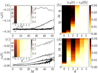
Figure 2: Quantum energy dynamics for line defects created in the $\ket{\rightarrow}$ (upper panel) and $\ket{\rightarrow}_{\mathrm{FF}}$ (lower panel) initial states, displaying the normalized plaquette energy $\varepsilon_{d}(t)$ of $d$-th column. (a,c) $\varepsilon_{d}(t)$ for different columns $d=2\div 5$ where darker colors refer to larger distances from the initial defect. Insets show the same data including $d=0,1$ in a color plot. (b,d) Absolute deviation of $\varepsilon_{d}(t)$ from the initial value $\varepsilon_{d}(0)$. (b) Signal propagation for $\ket{\rightarrow}$ showing a strong bending of the light cone indicating localized behavior and (d) for $\ket{\rightarrow}_{\mathrm{FF}}$ consistent with linear propagation indicative of ergodic behavior. For all the plots $J/\lambda=-0.1$ and system size $10\times 10$.

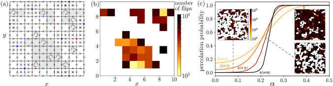
Figure 3: Classical correlated percolation problem implying a quantum nonergodic phase in the QLM. (a) Typical spin configuration sampled from $|\rightarrow\rangle$ with arrows showing the local spin orientation and circular arrows flippable plaquettes. Red and blue disks denote positive and negative background charges, respectively. Crosses indicate plaquettes blocked by charges $q=\pm 2$. Grey color indicates plaquettes that can become flippable in the course of the evolution. (b) Result of the Monte Carlo simulation starting from the state (a). The colormap shows the number of times that the individual plaquettes were flipped in the course of the simulation; white color stands only for plaquettes, that have never been flipped. c) Percolation probability vs $\alpha$. The insets show typical configurations below, at, and above the percolation threshold $\alpha_{c}\approx 0.25$ for a $40\times 40$ system.

Localized and ergodic dynamics. Using the vCNs we now compute nonequilibrium dynamics in the QLM. We start by studying the spatiotemporal buildup of quantum correlations, measured via $\langle S^{z}_{0}(t)S^{z}_{d}(t)\rangle$, upon initializing the system in state $\ket{\psi_{0}}=\ket{\rightarrow}$. The result is shown in Fig. 1(b), where one can see that correlations emerge only over a limited spatial distance suggesting nonergodic behavior. We proceed by further corroborating this observation by other measures.

Namely, we study energy transport in the QLM by creating initial conditions with a spatial energy inhomogeneity in the form of a line defect with subextensive energy contribution and use the character of energy propagation to distinguish between ergodic and localized dynamics. Concretely, we consider the two initial conditions $\ket{\psi_{0}}=\ket{\rightarrow}$ or $\ket{\rightarrow}_{\mathrm{FF}}$ upon applying in addition $P=\prod_{\square\in\mathcal{C}_{0}}[1+(U_{\square}+U_{\square}^{\dagger})^{2}]$ along all plaquettes in column $d=0$; here $\mathcal{C}_{d}$ denotes the set of plaquettes in column $d$. In Fig. 2 we plot the (normalized) column energy $\varepsilon_{d}(t)=(\langle H_{d}(t)\rangle-H_{\mathrm{av}})/H_{\mathrm{av}}$ with $H_{d}=\sum_{\square\in\mathcal{C}_{d}}H_{\square}$ the total energy for the plaquettes in $d$-th column, $H_{\square}=\lambda(U_{\square}+U_{\square}^{\dagger})^{2}-J(U_{\square}+U_{\square}^{\dagger})$. Further, $H_{\mathrm{av}}=\langle H\rangle/L$ denotes the expected $\langle H_{d}(t)\rangle$ in the long-time limit when the system is thermalizing ($L$ is the number of columns).

Comparing Figs. 2(a) and (c) we observe that the dynamics differs qualitatively for the two initial conditions, although the Hamiltonian parameters are identical. While for $|\psi_{0}\rangle=\ket{\rightarrow}$ energy transport is highly suppressed and only visible on short distances (Fig. 2(a)), the opposite happens for $\ket{\rightarrow}_{\mathrm{FF}}$. This becomes even more apparent in Figs. 2(b,d), where $\varepsilon_{d}(t)$ relative to the initial value $\varepsilon_{d}(0)$ is shown, therefore more directly highlighting energy propagation. While for $\ket{\rightarrow}_{\mathrm{FF}}$ we identify a linearly propagating front, for $\ket{\rightarrow}$ we observe a strong bending. We argue below that this front for $\ket{\rightarrow}$ can extend only to a finite region as a consequence of disorder-free localization.

Bound on quantum dynamics by unconventional percolation. The qualitative difference in the quantum dynamics for the initial states $\ket{\rightarrow}$ and $\ket{\rightarrow}_{\mathrm{FF}}$ originates from a dynamical transition, which one can study systematically upon tuning the parameter $\alpha$ for the initial state (2). For this purpose, we employ an unconventional correlated classical percolation problem Coniglio:2009 and establish a bound on the quantum localized-ergodic transition in the QLM providing a numerical proof for an extended nonergodic phase as a consequence of disorder-free localization.

We illustrate the idea for the initial state $\ket{\rightarrow}$, distributed over all superselection sectors. Consider a typical (random) sector from this distribution (Fig. 3(a)). Such sector exhibits many background charges $q_{\mathbf{r}}$ whenever the “two-in two-out” rule at vertex $\mathbf{r}$ is violated. Importantly, these background charges (constants of motion by gauge invariance) impose strong kinetic constraints. For instance, $q_{\mathbf{r}}=\pm 2$ implies that neighboring spins either all point inwards or outwards, hence the adjacent plaquettes remain unflippable forever. The influence of $q_{\mathbf{r}}=\pm 1$ charges is more subtle. They make at least $2$ adjacent plaquettes unflippable, while their positions might change over time.

The question we address now is whether these constraints are so strong to fragment the square lattice into sets of kinetically disconnected islands or whether one can contain an extensive (percolating) connected cluster. For that purpose we study an unconventional percolation problem using an infinite-temperature classical MC simulation. We start from the initial condition (2), sampling a random basis state (and thus a sector) with a distribution set by the amplitudes in $|\psi(\alpha)\rangle$. Then we determine which parts of the systems are kinetically connected, using MC search with random plaquette flips. The simulation is stopped when every plaquette is flipped either 0 or more than some fixed threshold ($=100$) number of times (or after $10^{11}$ MC steps if this condition is still not satisfied). As a result we find the number of performed flips for each plaquette (Fig. 3(b)). Repeating this procedure for different initial configurations at a given $\alpha$ and scanning $\alpha$, we finally obtain the percolation probability (Fig. 3(c)). Most importantly, one can observe a clear evidence for a percolation threshold $\alpha_{c}\approx 0.25$. Although the simulation termination condition is chosen such as to minimize the number of potentially missed “weak connections” between flippable clusters, we cannot exclude the possibility of such misses. While we don’t expect a significant impact deep in the respective phases, this caveat might become important in the vicinity of $\alpha_{c}$, preventing us to obtain a precise value of $\alpha_{c}$ and to study the critical behavior.

Since $\alpha_{c}>0$, the initial state $\ket{\psi(\alpha=0)}=\ket{\rightarrow}$ corresponds to the classically non-percolating side of the transition, while from $\alpha_{c}<\pi/4$ it follows that state $\ket{\psi(\alpha=\pi/4)}=\ket{\mathrm{FF}}$ and all other states from the FF-sector (including $\ket{\rightarrow}_{\mathrm{FF}}$) lie on the percolating side. This classical threshold is imprinted in the quantum dynamics and ultimately leads to the strong localization observed in propagation of correlations (Fig. 1(b)) and of the energy (Fig. 2(a),(b)) for $\ket{\rightarrow}$. For the FF-sector state $\ket{\rightarrow}_{\mathrm{FF}}$ there is no percolation constraint, which allows propagation of the signal to long distances (Fig. 2(c),(d)). This analysis sets a lower bound onto the critical value of the quantum transition $\alpha_{c}^{(q)}$, since the quantum system might be still localized due to interference even on the classically percolating side.

Summary and outlook. We have shown that genuinely interacting 2D homogeneous LGTs can become nonergodic as a consequence of disorder-free localization. This is all the more surprising as many-body localization is predicted to be unstable in 2D at elevated energy densities Deroeck:2017 , implying that gauge invariance represents a more robust mechanism of ergodicity breaking compared to conventional disorder. The key element of our analysis is a bound on the localization-delocalization transition based on a classical correlated percolation problem implying a strong fragmentation of Hilbert space into kinetically disconnected regions. Both the percolation analysis as well as the introduced variational classical networks can be directly applied to other quantum many-body systems with finite-dimensional local Hilbert spaces independent of dimensionality, such as 3D quantum spin ice systems, which might be an interesting scope of the developed techniques in the future. Further, it might be interesting to explore how the quantum and classical percolation thresholds are related to each other as well as to determine their respective critical behaviors, and whether the disorder-free localization scenario holds also in the presence of matter degrees of freedom. Our theoretical analysis appears within reach of future experiments: significant efforts in the last years have explored routes to realize the QLM model experimentally in systems of Rydberg atoms Celi:2019 ; Glaetzle:2014 as a next step after the recent experimental advances on 1D LGTs Martinez:2016 ; Kokail:2019 ; Esslinger:2019 ; Aidelsburger:2019 ; Mil:2019 .

Acknowledgments. We are grateful to H. Burau, J. Chalker, M. Dalmonte, R. Moessner, and G.-Y. Zhu for helpful discussions. P.K. acknowledges the support of the Alexander von Humboldt Foundation and the Ministry of Science and Higher Education of the Russian Federation. This project has received funding from the European Research Council (ERC) under the European Union’s Horizon 2020 research and innovation programme (grant agreement No. 853443), and M. H. further acknowledges support by the Deutsche Forschungsgemeinschaft via the Gottfried Wilhelm Leibniz Prize program. Y.-P.H. receives funding from the European Union’s Horizon 2020 research and innovation program under the Marie Skłodowska-Curie grant agreement No. 701647. M.S. was supported through the Leopoldina Fellowship Programme of the German National Academy of Sciences Leopoldina (LPDS 2018-07) with additional support from the Simons Foundation.

References

- (1) D.S. Rokhsar and S.A. Kivelson, Phys. Rev. Lett. 61, 2376 (1988).
- (2) M.J.P. Gingras and P.A. McClarty, Rep. Prog. Phys. 77, 056501 (2014)
- (3) M. Stern, C. Castelnovo, R. Moessner, V. Oganesyan, and S. Gopalakrishnan, arXiv 1911.05742.
- (4) Lattice Gauge Theories: An Introduction (3nd ed.), H.J. Rothe (World Scientific, 2005).
- (5) C.J. Turner, A.A. Michailidis, D.A. Abanin, M. Serbyn, and Z. Papic, Nat. Phys. 14, 745 (2018)
- (6) C.-J. Lin and O.I. Motrunich, Phys. Rev. Lett. 122, 173401 (2019)
- (7) M. van Horssen, E. Levi, and J.P. Garrahan, Phys. Rev. B 92, 100305(R) (2015).
- (8) N. Pancotti, G. Giudice, J I. Cirac, J.P. Garrahan, and M.C. Banuls, arXiv:1910.06616.
- (9) Z. Lan, M. van Horssen, S. Powell, and J.P. Garrahan, Phys. Rev. Lett. 121, 040603 (2018).
- (10) P. Sala, T. Rakovszky, R. Verresen, M. Knap, and F. Pollmann, arXiv 1904.04266.
- (11) S. Pai and M. Pretko, Phys. Rev. Lett. 123, 136401 (2019).
- (12) S. Pai, M. Pretko, and R.M. Nandkishore, Phys. Rev. X 9, 021003 (2019).
- (13) V. Khemani and R. Nandkishore, arXiv:1904.04815.
- (14) A. Smith, J. Knolle, D.L. Kovrizhin, and R. Moessner, Phys. Rev. Lett. 118, 266601 (2017).
- (15) A. Smith, J. Knolle, R. Moessner, and D.L. Kovrizhin, Phys. Rev. Lett. 119, 176601 (2017).
- (16) M. Brenes, M. Dalmonte, M. Heyl, and A. Scardicchio, Phys. Rev. Lett. 120, 030601 (2018).
- (17) I.H. Kim and J. Haah, Phys. Rev. Lett. 116, 027202 (2016).
- (18) A. Smith, J. Knolle, R. Moessner, and D.L. Kovrizhin, Phys. Rev. B 97, 245137 (2018).
- (19) U.-J. Wiese, Annalen der Physik 525, 777 (2013).
- (20) S. Chandrasekharan and U.-J. Wiese, Nuclear Physics B 492, 455 (1997).
- (21) N. Shannon, G. Misguich, and K. Penc, Phys. Rev. B 69, 220403(R) (2004).
- (22) M. Hermele, M.P.A. Fisher, and L. Balents, Phys. Rev. B 69, 064404 (2004).
- (23) D. Banerjee, F.-J. Jiang, P. Widmer, and U.-J. Wiese, J. Stat. Mech P12010 (2013).
- (24) A. Celi, B. Vermersch, O. Viyuela, H. Pichler, M.D. Lukin, P. Zoller, arXiv 1907.03311.
- (25) A. Glaetzle, M. Dalmonte, R. Nath, I. Rousochatzakis, R. Moessner, and P. Zoller, Phys. Rev. X 4, 041037 (2014).
- (26) G. Carleo, M. Troyer, Science 355, 602 (2017).
- (27) M. Schmitt and M. Heyl, SciPost Phys. 4, 013 (2018).
- (28) R. Kubo, Generalized Cumulant Expansion Method, J. Phys. Soc. Jpn. 17, 1100 (1962).
- (29) See the Supplementary Material.
- (30) R. Verdel, P. Karpov, Y.-P. Huang, M. Schmitt and M. Heyl, to appear.
- (31) M. Schmitt and M. Heyl, arXiv:1912.08828.
- (32) A. Coniglio, A. Fierro. Correlated Percolation. In: Meyers R. (eds) Encyclopedia of Complexity and Systems Science (Springer, New York, 2009).
- (33) W. De Roeck and J. Z. Imbrie, Philos. Trans. Royal Soc. A 375, 20160422 (2017).
- (34) E. Martinez, C. Muschik, P. Schindler, D. Nigg, A. Erhard, M. Heyl, P. Hauke, M. Dalmonte, T. Monz, P. Zoller, and R. Blatt, Nature 534, 516 (2016).
- (35) C. Kokail, C. Maier, R. van Bijnen, T. Brydges, M. K. Joshi, P. Jurcevic, C. A. Muschik, P. Silvi, R. Blatt, C. F. Roos, et al., Nature 569 355, (2019).
- (36) F. Görg, K. Sandholzer, J. Minguzzi, R. Desbuquois , M. Messer and T. Esslinger, Nature Physics 15, 1161 (2019).
- (37) C. Schweizer, F. Grusdt, M. Berngruber, L. Barbiero, E. Demler, N. Goldman, I. Bloch, and M. Aidelsburger, Nature Physics 15, 1168 (2019).
- (38) A. Mil, T.V. Zache, A. Hegde, A. Xia, R.P. Bhatt, M.K. Oberthaler, P. Hauke, J. Berges, and F. Jendrzejewski, arXiv:1909.07641.