Abstract

The depth-dependent abundance of both gas-phase and solid-state water within dense, quiescent molecular clouds is important to both the cloud chemistry and gas cooling. Where water is in the gas phase, it’s free to participate in a network of ion-neutral reactions that lead to a host of oxygen-bearing molecules, and its many energy levels make it an effective coolant for gas temperatures $\geq\>$20 K. Where water is abundant as ice on grain surfaces, and unavailable to cool the gas, significant amounts of oxygen are removed from the gas phase, suppressing the gas-phase chemical reactions that lead to a number of oxygen-bearing species, including O₂. Models of FUV-illuminated clouds predict that the gas-phase water abundance peaks within A_V$\,\sim\,$3 and 8 mag. of the cloud surface, depending on the gas density and FUV field strength. Deeper within such clouds, water is predicted to exist mainly as ice on grain surfaces. More broadly, these models are used to analyze a variety of other regions, including outflow cavities associated with young stellar objects and the surface layers of protoplanetary disks. In this paper, we report the results of observational tests of FUV-illuminated cloud models toward the Orion Molecular Ridge and Cepheus B using data obtained from the Herschel Space Observatory and the Five College Radio Astronomy Observatory. Toward Orion, 2,220 spatial positions were observed along the face-on Ridge in the H₂O 1${}_{10}\,$– 1₀₁ 557 GHz and NH₃ $J,K=\>$1,0 – 0,0 572 GHz lines. Toward Cepheus B, two strip scans were made in the same lines across the edge-on ionization front. These new observations demonstrate that gas-phase water exists primarily within a few magnitudes of dense cloud surfaces, strengthening the conclusions of an earlier study based on a much smaller dataset, and indirectly supports the prediction that water ice is quite abundant in dense clouds.

1. Harvard-Smithsonian Center for Astrophysics, 60 Garden Street, MS 66, Cambridge, MA 02138, USA
   

2. Department of Astronomy, University of Massachusetts, Amherst, MA 01003, USA
   

3. Department of Physics and Astronomy, San José State University, San Jose, CA 95192, USA
   

4. Department of Astronomy, The University of Michigan, 500 Church Street, Ann Arbor, MI 48109-1042, USA
   

5. IFF, Consejo Superior de Investigaciones Cientificas (CSIC), 28049 Madrid, Spain
   

6. Jet Propulsion Laboratory, California Institute of Technology, 4800 Oak Grove Drive, Pasadena, CA 91109, USA
   

7. Universidad de Alcalá de Henares, Departamento de Física, Campus Universitario, E-28871 Alcalá de Henares, Madrid, Spain
   

8. SETI Institute, Mountain View, CA 94043, USA
   

9. Department of Physics and Astronomy, Johns Hopkins University, 3400 North Charles Street, Baltimore, MD 21218, USA

1 INTRODUCTION

The distribution of gas-phase water within dense ($n$(H₂) $\stackrel{{\scriptstyle\textstyle>}}{{\sim}}$ 10${}^{3}\>$cm^-3) molecular clouds is of interest since it affects both the oxygen chemistry and cooling within the gas. In particular, where water is present in the gas phase, it is free to participate in ion-neutral chemical reactions that affect the distribution of oxygen among species such as O, OH, O₂, and CO. Where water is present as ice, which results from the freeze-out of gas-phase water onto dust grains or direct formation on grain surfaces via the repeated hydrogenation of O, the $\stackrel{{\scriptstyle\textstyle>}}{{\sim}}$ 90 K sublimation temperature required to release water from these grains effectively means that within cold (i.e., $\stackrel{{\scriptstyle\textstyle<}}{{\sim}}$ 30 K) dense clouds, water, and the oxygen it contains, remains locked as ice and unavailable for further reactions in the gas phase.

In an earlier study (Melnick et al., 2011, henceforth Paper I), ground-state 1${}_{10}\,$– 1₀₁ ortho-H₂O 557 GHz observations obtained using the Submillimeter Wave Astropnomy Satellite (SWAS) and millimeter-wave spectral line observations obtained using the Five College Radio Astronomy Observatory (FCRAO) were used to determine the depth-dependent distribution of gas-phase water toward the face-on Orion Molecular Cloud ridge, located at a distance of 412 pc (Reid et al., 2009). The present work reexamines the results of this previous study, using instead 1${}_{10}\,$– 1₀₁ ortho-H₂O observations obtained with the Herschel Space Observatory. Because of its larger aperture (and smaller beam size) and greater sensitivity, Herschel was able to sample 2,220 spatial positions along the Orion ridge whereas SWAS sampled only 77 spatial positions over approximately the same area.

As noted in the earlier study, establishing the distribution of gas-phase water within dense molecular clouds is important for at least two reasons. First, the depth-dependent abundance of gas-phase water is sensitive to the efficiency of several key processes, such as photodissociation, photodesorption, gas-phase reactions, gas-grain reactions, and grain-surface reactions, most of which depend upon the gas density and far-ultraviolet (FUV) flux (6 eV $<$ $h\nu$ $<$ 13.6 eV). The relative importance of these processes remain somewhat uncertain. Second, because oxygen is the most abundant element after hydrogen and helium, the processes that control the amount of oxygen locked in both water vapor and water ice determine the amount of residual oxygen free to react with other species. In this way, the predicted abundance of a host of species that depend on the gas-phase oxygen-to-carbon or oxygen-to-nitrogen ratio hinges on knowledge of the main reservoirs of oxygen, such as gas-phase water and water ice. In their study of the distribution of gas- and ice-phase water within molecular clouds, Hollenbach et al. (2009) found that, over a broad range of cloud densities, i.e., $n=\>$10³ – 10${}^{5}\>$cm^-3, and external FUV field intensity, i.e., 1 – 10³ times the average local interstellar radiation field in the FUV band (Habing, 1968) – gas-phase water remains largely a cloud surface phenomenon. This conclusion was supported by the earlier SWAS data (Paper I); however, the availability of a substantially improved Herschel dataset warrants a reexamination of the question.

In addition to Orion, we also present here results obtained toward the Cepheus B molecular cloud. The Cepheus B molecular cloud is at a distance of approximately 725 pc and located adjacent to the Cepheus OB3 association. The interface between the molecular cloud and the OB association is clearly delineated by the optically visible HII region S155. S155 has a very sharp western edge indicating the presence of an ionization front bounding the molecular cloud. The ionizing radiation in this region is dominated by two hot and luminous stars: the O7 n star HD 217086 and the Be star HD 217061. Whereas the photodissociation region (PDR) in Orion is viewed face-on, the Cepheus B PDR displays an edge-on geometry and an opportunity to map the distribution of water through spatial strip scans.

A number of previous investigations have invoked line-of-sight distributions of gas-phase and solid water for the purpose of fitting observed line profiles (e.g., Cernicharo et al., 2006; Caselli et al., 2012; Coutens et al., 2012; Mottram et al., 2013; Keto, Rawlings & Caselli, 2014; Schmalzl et al., 2014). The results of these studies are useful as they provide critical tests of chemical and dynamical models, often involving a mixture of quiescent envelopes, embedded heat sources and, in some cases, infall or outflow motions, along relatively few sight lines. However, whether it’s line-of-sight complexity, the limited number of sight lines, or both, such observations make it difficult to judge whether the predictions of chemical models of UV-illuminated dense, quiescent clouds and observations broadly agree. The intent of this study is to utilize more than 2000 lines of sight to present a statistically robust observational study of the distribution of water vapor toward portions of the dense (i.e., $n$(H₂) $\stackrel{{\scriptstyle\textstyle>}}{{\sim}}$ 10⁴ cm^-3) Orion Molecular Cloud ridge possessing no known embedded sources or outflows, and the fortuitous geometry of Cepheus B, to determine whether the presence of gas-phase water predominantly near molecular cloud surfaces is a ubiquitous property reflective of the processes outlined above.

In §2 we discuss the observations. In particular, in §2.1, we discuss the observations toward the Orion Molecular Cloud and, in §2.2, we discuss the observations toward Cepheus B. In §3 we present our findings. The results toward Orion are given in §3.1, including the Herschel maps obtained in H₂O and NH₃ (§3.1.1); the determination of the visual extinction, A_V, toward the Orion Ridge (§3.1.2); the line optical depths, CO depletion, the relation between the ¹³CO column density and A_V (§3.1.3); the depth-dependent line intensity ratios(§3.1.4); a Principal Component Analysis (PCA) of the lines observed (§3.1.5); and, the H₂O Integrated Intensity vs. A_V for a Range of $G_{\rm o}$ and $n_{\rm H}$ (§3.1.6). In §3.2 we present the results of the strip scans toward Cepheus B. In §4, we discuss the implications of these results on our understanding of water in dense clouds and the interpretation of observatons of gas-phase water.

2 OBSERVATIONS

2.1 Orion Molecular Cloud

The Herschel/HIFI observations of the Orion-KL region presented here were carried out on 2011 September 15 (ObsID: 1342228626). A 25^′$\,\times\,$40^′ region was mapped in the 1₁₀  – 1₀₁ rotational transition of H₂O at 556.936 GHz in Band 1b simultaneously in H- and V-polarization. The map was centered at $\alpha=\>$5^h 35^m 20.5^s and $\delta=-$5^o 17^′ 7^′′. HIFI (Roelfsema et al., 2012) was used in On-The-Fly (OTF) Maps observing mode with position-switch reference located at $\alpha=\,$5^h 32^m 25.9^s and $\delta=-$5^o 22^′ 36.80^′′ (J2000). The angular separation between adjacent scans was $\sim\,$40^′′, a compromise between area covered and spatial resolution. The HIFI receivers are sensitive to signals in both sidebands. Thus, the local oscillator (LO) frequency could be selected such that the (J,K)$\>=\>$(1,0) – (0,0) transition of ortho-NH₃ at 572.498 GHz could be observed simultaneously with H₂O. The wide band spectrometer (WBS) provided a spectral resolution of 1.1 MHz corresponding to a velocity width of $\sim\,$0.6 km s^-1 for the 556.9 GHz line. The total on-source integration time per map point (for each polarization) was 5.92 sec. and the total mapping time was 5.1 hours. The Herschel telescope beam FWHM is $\sim\,$37^′′ at 557 GHz and 572 GHz, the main beam efficiency (Mueller et al., 2014) is 0.62, and the ratio of Lower Sideband (LSB) to Upper Sideband (USB) gain is 0.54:0.46 at these frequencies (Kester, Higgins & Teyssier, 2017). All values were extracted from the Observation Context HIFI Calibration Data Set (HIFI_CAL_25_0).

All HIFI data were processed using the Herschel Interactive Processing Environment (HIPE) (Ott, 2010), Version 10.3, up to Level 2 providing fully calibrated spectra with the intensities expressed as antenna temperature and the frequencies in the frame of the Local Standard of Rest (LSR). Further data processing steps in HIPE included running FitHifiFringeTask and applying the main beam efficiency before saving the data in CLASS-FITS format. The overall data quality was excellent with only minor low-intensity ripples in some scans.

Since the initial extensive analysis, the data reduction software HIPE has been upgraded to version 15.0. In order to avoid the need to redo the data reduction and analysis, we updated our data sets to bring them into conformity with data reduced in HIPE, Version 15.0. These updates included changing the receiver sideband ratios and the main beam efficiency to the values listed above and comparing random spectra (with line emission) reduced in HIPE Version 10.3 with the same spectra reduced in HIPE 15.0. The observed differences were sufficiently small (i.e., $<\,$3%) so as to have no impact on the analysis.

In 2004, maps of the emission from C₂H, HCN, N₂H⁺, and CN toward Orion were obtained with the 14-meter telescope of the Five College Radio Astronomy Observatory (FCRAO). In April 2005, further observations were obtained in C₂H and N₂H⁺ repeating regions in Orion where the emission was weak. All lines were observed using the On-The-Fly observing method. The 32-pixel SEQUOIA array receiver (Erickson et al. 1999) was used to observe two lines simultaneously. The spectrometer for each spatial pixel was a digital autocorrelator with a bandwidth of 50 MHz and 1024 spectral channels per pixel leading to a velocity channel spacing that varied between 0.13 and 0.17 km s^-1 depending on the line frequency. The observations were first reduced to form maps with data spaced by 20^′′. The FWHM beam size of the FCRAO telescope varies from approximately 46^′′ at the CN line frequency to 56^′′ at the C₂H line frequency. The main beam efficiency, $\eta_{\rm mb}$, of the FCRAO antenna varies from approximately 0.45 (at 115 GHz) to 0.48 (at $\sim\,$88 GHz).

The ¹²CO and ¹³CO data used for this analysis are the same as described in Ripple et al. (2013), who also used the FCRAO 32-pixel SEQUOIA array receiver during 2005 and 2006. Both lines were observed simultaneously using the On-The-Fly observing method. However, they used the autocorrelator with 25 MHz bandwidth and a spectral channel spacing of 0.077 km s^-1 and 0.080 km s^-1 at the ¹²CO and ¹³CO line frequencies, respectively. For the analysis, the spectral channels were resampled to a spacing of 0.2 km s^-1. The FWHM beam sizes of the FCRAO telescope are approximately 45^′′ and 47^′′ and the main beam efficiencies are 0.45 and 0.48 at the ¹²CO and ¹³CO line frequencies, respectively. For more details see Ripple et al. (2013). A summary of the Herschel/HIFI and FCRAO observations is provided in Table 1. The maps obtained with the FCRAO telescope are shown in Fig. 1.

In order to directly compare the data obtained from Herschel/HIFI and FCRAO, all data were first regridded onto a common spatial grid with equal beam sizes. Since the area covered by the FCRAO maps exceeds those of the Herschel/HIFI observations, the latter determined the extent of the final maps. The regridded maps have 24 $\times$ 40 spatial pixels on a 1^′ grid and beam sizes that were convolved to a FWHM of 1^′, slightly larger than the largest beam of the observations (see Table 1), using appropriate Gaussian kernels. The spatial positions of the regridded data are shown in Fig. 2.

The integrated intensities were derived in two steps. First, Gaussian fits to the continuum-subtracted line profiles of all the species listed in Table 1 were obtained. In many cases, these fits involved multiple velocity components including, for HCN, CN, C₂H, and N₂H⁺, hyperfine components of known velocity separation (from the main component) and common FWHM (to the main component).

In the second step, a direct, summed integrated intensity was obtained for each molecule and map position. To do so, the fitted line centers and FWHM’s of each ¹³CO velocity component were used to set the velocity ranges within each spectrum in which the flux in each spectral resolution element was directly summed. Specifically, the region within each spectrum directly summed was bounded by the ¹³CO component with the lowest velocity, minus 1.3 times the FWHM of this component, to the ¹³CO component with the highest velocity, plus 1.3 times its FWHM. Thus, the data set for further analysis included the fit results and integrated intensities of all individual ¹³CO velocity components together with the summed integrated intensities over the full velocity range, as described above, for all other species. The first step was necessitated by the desire to derive line-center optical depths along with the total column density of ¹³CO toward each spatial position (see Ripple et al., 2013, eqns. (1) – (5)), as well as to examine the connection between the LSR velocities of all the observed species. The second step, i.e., direct integration of the spectra to determine the integrated intensities, was necessitated by the desire to include the flux contribution from noisy, but net positive, spectral lines whose Gaussian fits were either difficult or impossible to obtain. As will be discussed, species whose abundance (and emission) peak within a relatively narrow range of A_V’s will produce weak lines toward lines of sight with lower H₂ densities. Nevertheless, such lines contain useful information that can be retrieved through direct integration.

2.2 Cepheus B Molecular Cloud

The Herschel/HIFI observations of Cepheus B were carried out on 2012 May 8 and 2012 May 24. Observations of the 557 GHz line of water were obtained in two strip scans using the OTF mapping mode of Herschel. A northern strip map (ObsIDs: 1342245588) was centered at RA (J2000) = 22^h 57^m 16^s and Dec (J2000) = +62^o 35^′ 45^′′ and covered a range in right ascension from 193.3 arcseconds west to 189.0 arcseconds east of the center. A southern strip map (ObsID: 1342246073) was centered at RA (J2000) = 22^h 57^m 24^s and Dec (J2000) = +62^o 34^′ 45^′′ and covered a range in right ascension from 192.9 arcseconds west to 190.1 arcseconds east of the center. The HIFI receiver setup for both observations was the same as for the Orion-KL observations described above.

Observations of the 572 GHz line of NH₃ were obtained simulataneously with those of H₂O in the other sideband of the water line. These data were reduced using HIPE in the same manner as described in §2.1. The two strip maps were scanned along an east-west line and included 81 samples spaced by 5^′′, the two strip maps were offset in declination by one arcminute. The location of the strip maps are shown in Fig. 3 superimposed on an image of the region.

The data from the H- and V-beams, separated by $\sim\,$4^′′ orthogonal to the OTF scan direction were coadded. Nevertheless, the signal to noise in the coadded spectra was still relatively low. We therefore averaged the spectra along each strip map in groups of seven spectra (with equal weighting) forming a new spectrum every fourth spectrum. The resulting new strip maps have 19 spectra along the northern scan and 20 spectra along the southern scan spaced by 20^′′ and averaged over 30^′′ (approximately the Herschel beam at 557 GHz and much larger than the H- and V-beam separation). In Fig. 4, we show plots of the resulting integrated intensity of the water and ammonia lines as a function of offset from the center position for the northern strip map, while Fig. 5 shows the same for the southern strip map. The integration was performed over a velocity range of -20 to -10  km s^-1, except for a few spectra that showed broad wings, in which the velocity range was extended to -30 to 0  km s^-1.

In the course of making the strip maps, a broad water emission source was discovered in several of the spectra in both strip maps. Fig. 6 shows the water spectrum toward one of these positions. This previously unreported outflow is discussed in §3.2.

3 RESULTS

3.1 Orion Molecular Cloud

3.1.1 Water and Ammonia Maps

Fig. 7 shows the Herschel/HIFI ortho-H₂O 556.936 GHz 1${}_{10}\,$– 1₀₁ summed integrated intensity map toward the Orion Molecular Ridge. Fig. 8 shows the Herschel/HIFI ortho-NH₃ 572.498 GHz (J,K)$\,=\,$(1,0) – (0,0) summed integrated intensity map toward the same region.

3.1.2 A_V Determination

In Paper I, the relation between the C¹⁸O column density, $N$(C¹⁸O), and A_V was based on studies of dark clouds, such as Chamaeleon I and III-B (Kainulainen, Lehtinen, & Harju, 2006) using Two-Micron All Sky Survey (2MASS) data. More recently, Ripple et al. (2013) studied the relationship between $N$(¹³CO) and visual extinction toward the Orion A and Orion B molecular clouds. They computed the ¹³CO column density in these clouds from observations of the ¹²CO $J=$1 – 0 and ¹³CO $J=$1 – 0 transitions assuming LTE. The visual extinction was determined directly from photometry of background stars using the 2MASS database and used to establish the correlation between $N$(¹³CO) and A_V. They find three distinct regimes of A_V in which the ratio of ¹³CO column density and visual extinction differ. At low A_V’s (Regime 1), in the photon-dominated envelope, the column density of ¹³CO is low, but increases into the well-shielded interior of the clouds at higher A_V’s (Regime 2). At the highest A_V’s (Regime 3), some regions of the cloud, particularly those with dust temperatures below $\sim$ 22 – 25 K, show evidence of a flattening of the ¹³CO integrated intensity, which is attributed to CO depletion.

Based on our determination of $N$(¹³CO), we estimate the visual extinction using the results from Ripple et al. (2013). In the Ripple et al. study, the Orion A cloud is divided into a number of partitions, where each partition corresponds to a distinct spatial region within the larger Orion complex. Partition 6 of their study corresponds to the region of the Orion A cloud investigated in this paper. Within this partition, Ripple et al. find no evidence for CO depletion. This finding is in agreement with the conclusion drawn in Paper I.

The relation between $N$(¹³CO) and A_V for Partition 6 is given by Ripple et al. as:

$$A_{V}({\rm mag.})=~{}2.0\times 10^{-15}~{}N({\rm{}^{13}CO})\,-\,0.5~{}~{}~{}~{}{\rm for}~{}2.5\times 10^{14}~{}{\rm cm^{-2}}<N({\rm{}^{13}CO})<2.1\times 10^{15}~{}{\rm cm^{-2}}\\$$ (1)

$$A_{V}({\rm mag.})=~{}2.78\times 10^{-16}~{}N({\rm{}^{13}CO})\,+\,3.12~{}~{}~{}~{}~{}{\rm for}~{}N({\rm{}^{13}CO})>2.1\times 10^{15}~{}{\rm cm^{-2}}\hskip 28.45274pt\phantom{0}$$ (2)

Within the low column density regime, as expressed in Eqn. (1), $N$(¹³CO) grows very slowly with increasing A_V, consistent with the photodestruction of ¹³CO near the cloud surface. Ripple et al. derived Eqn. (1) based on an empirical fit to $N$(¹³CO) and A_V data and we note that values of $N$(¹³CO)$\><\>$2.5$\,\times\,$10¹⁴ cm^-2 would imply an unphysical value for A_V. However, of the 898 map positions used to construct the water map shown in Fig. 7, only two positions have $N$(¹³CO) values less than 2.5 $\,\times\,$10¹⁴ cm^-2. These positions are located at the east edge of the map and have no associated H₂O emission and, thus, do not factor into the analysis that follows. In fact, all but four map positions have $N$(¹³CO)$\;>\;$4$\,\times\,$10¹⁴ cm^-2 resulting in values of A_V$\,>\>$0.3 mag.

As the depth into the cloud increases, as expressed in Eqn. (2), and self shielding becomes effective, $N$(¹³CO) exhibits a steeper linear growth with A_V. Ripple et al. find that in Partition 6 (Orion A), a significant fraction of ¹³CO remains in the gas phase to at least A_V $=\>$25 mag. Fig. 9 shows the map of A_V generated using Eqns. (1) and (2) and the ¹³CO column densities derived from the FCRAO data obtained here.

3.1.3 Line Optical Depths

The analyses in the following sections assume that the line-center optical depths are less than 1. Here we show this to be the case for ¹³CO, C¹⁸O, HCN, N₂H⁺, CN, and C₂H.

The line-center optical depth of the ¹³CO (1 – 0) transition can be expressed as:

$$\tau(^{13}{\rm CO})=-{\rm ln}\left[1-\frac{T_{\rm max}(^{13}{\rm CO})/5.289\>{\rm K}}{1/\left(e^{\,5.289\,{\rm K}/T_{\rm ex}(^{13}{\rm CO})}-1\right)-0.16}\right]~{},$$ (3)

where 5.289 K $\equiv h\nu$ (¹³CO)$/k$, with $\nu$ (¹³CO)$\>=\>$110.201 GHz, the rest frequency of the ¹³CO (1 – 0) transition, $T_{\rm max\,}$(¹³CO) is the main beam brightness temperature at the peak of ¹³CO line (cf. Ripple et al., 2013), and $T_{\rm ex}$(¹³CO) is the ¹³CO excitation temperature. As discussed in Section 3.1.6, the H₂ densities required to account for the measured H₂O line emission vary between about 3$\,\times\,$10⁴ cm^-3 and 10⁵ cm^-3. Based on a grid of RADEX models within this range of densities, gas temperatures between 20 K and 35 K, and column densities corresponding to A_V’s between 3 and 30, the average excitation temperature of the ¹³CO (1 – 0) line is the same as that of the ¹²CO (1 – 0) line to within about 3%, and $T_{\rm ex}$ is thus given by

$$T_{\rm ex}=\frac{5.532~{}{\rm K}}{{\rm ln}\left[1+5.532\>{\rm K}/\left(T_{\rm max}(^{12}{\rm CO})+0.8363\>{\rm K}\right)\right]}$$ (4)

where 5.532 K $\,\equiv\,h\nu$(¹²CO)$/k$, with $\nu$(¹²CO)$\>=\>$115.271 GHz, the rest frequency of the ¹²CO (1 – 0) line. Based on the ¹²CO and ¹³CO FCRAO measurements described in §2.1, the ¹³CO line-center optical depths are almost all less than $\tau\,=\,$1. This is illustrated in Figs. 10 and 11.

The molecules HCN, N₂H⁺, CN, and C₂H have hyperfine structure that can be used to estimate the optical depth of these lines. We fitted the hyperfine components in these spectra using a template that fixes the relative velocities of the hyperfine components, assumes a common line width and Gaussian line shape. Thus, the free parameters for these fits are the intensities of the individual hyperfine components, one line velocity and one line width. These fits are then used to determine the intensity ratios of the various hyperfine components.

The hyperfine intensity ratio most sensitive to the optical depth is the ratio of the weakest hyperfine component to the strongest. For example, HCN has quadrupole hyperfine structure due to the spin of the nitrogen atom. The $J=$1 – 0 transition of HCN is split into three components, the F=2-1 feature is the strongest and the F=0-1 feature is the weakest. If these components are optically thin and in LTE, the expected intensity ratio is 0.20. In the upper-left panel of Fig. 12 we plot the F=0-1/F=2-1 intensity ratio versus the intensity of the strongest F=2-1 hyperfine component for HCN, where the error bars indicate the 1$\sigma$ uncertainty in the intensity ratio. Although there is considerable scatter and uncertainty in the ratio for the weaker intensity lines, as the lines become stronger, the ratio approaches the LTE optically thin value of 0.2. We would expect the strongest lines to be the most optically thick; however, they are the lines with intensity ratios consistent with the optically thin LTE ratio. Nevertheless, HCN has long been known to exhibit anomalous hyperfine ratios, as illustrated in the papers by Pirogov (1999) and Loughnane et al. (2012). Hyperfine ratios that include the F=1-1 component are often the most anomalous, while the F=0-1/F=2-1 ratio is usually more consistent with its LTE value, especially in higher mass molecular cloud cores. Despite this concern, the fact that the hyperfine ratios within the region studied here are consistent with an LTE ratio suggests that the HCN emission is optically thin.

Schilke et al. (1992) observed the isotopomer H¹³CN in several positions along the ridge in Orion, though all of their observed positions lie within the denser gas region close to BN/KL excluded from our analysis (see Fig. 2). Nevertheless, they found the isotopic line ratio HCN/H¹³CN to be of order 10, implying that the main isotopomer was optically thick. However, the intensity pattern of the hyperfine features in both isotopomers was roughly the same, which would be difficult to explain if HCN was optically thick. In fact, the modeling by Mullins et al. (2016) finds that, due to radiative transfer effects, the F$=$0-1 feature always appears stronger relative to the F$=$2-1 than predicted by LTE, just the opposite of what would be needed if HCN is optically thick. Schilke et al. suggest that fractionation of ¹³C is producing an increase in the ¹³C/¹²C ratio in HCN. Thus, the low observed isotopic ratio could be either due to HCN being optically thick, or due to fractionation. Since the hyperfine ratios could not be easily explained if HCN is optically thick, we believe that HCN is optically thin and fractionation is responsible for the small isotopic ratio.

The N₂H⁺ molecule also has quadrupole hyperfine structure produced by both nitrogen atoms. The outermost nitrogen atom produces three hyperfine components (denoted by the quantum number F1) that are very similar to that in HCN, while the innermost nitrogen atom is responsible for further splitting (denoted by the quantum number F) in two of these three components (Womack et al., 1992). However, the splitting produced by the innermost nitrogen atom is much less than the line width of the emission in Orion. Thus, these hyperfine features are blended, resulting in only three resolvable N₂H⁺ hyperfine components. The line strength ratios of the resolvable features are the same as those in HCN. In the lower-left panel of Fig. 12, we show the same hyperfine component ratios for N₂H⁺, i.e., F1=0-1/F1=2-1, as discussed above for HCN. The result is similar, except in the case of N₂H⁺, the intensity ratio approaches a value slightly greater than the optically thin LTE value of 0.2. As with HCN, anomalous hyperfine ratios have been found in N₂H⁺, and the study by Pirogov et al. (2003) of the hyperfine ratios in the $J=$1 – 0 transition of N₂H⁺ in massive molecular cloud cores obtained results similar to those we find in Orion. We also find that the F=1-1/F=2-1 intensity ratio is slightly lower than the optically thin LTE ratio of 0.6, as did Pirogov et al. (2003) in their study. The origin of these hyperfine anomalies in N₂H⁺ and HCN has been investigated by Keto & Rybicki (2010). Although we find small hyperfine anomalies in N₂H⁺, the F=0-1/F=2-1 intensity ratio still strongly suggests that the lines of N₂H⁺, like HCN, are optically thin.

In CN, we observe the F=3/2-3/2, F=1/2-1/2, F=5/2-3/2, and F=3/2-1/2 hyperfine components of the $N=$1 – 0 transition. The ratio of the weakest components (F=3/2-3/2 and F=1/2-1/2) to the strongest component (F=5/2-3/2) has an optically thin LTE ratio of 0.30. In the upper-right panel of Fig. 12 we plot the F=3/2-3/2/F=5/2-3/2 ratio versus the intensity of the F=5/2-3/2 component. As in the case for HCN, the data are consistent with the optically thin LTE ratio of 0.30. A plot using the F=1/2-1/2/F=5/2-3/2 intensity ratio is nearly identical to that shown. These results indicate that the CN emission is optically thin.

Finally, for the $N\!=\,$1 – 0 transition of C₂H, we observed the F=1-1 and F=0-1 hyperfine components. The optically thin LTE intensity ratio of F=0-1/F=1-1 is 0.4. The lower-right panel of Fig. 12 shows this ratio plotted versus the stronger F=1-1 component intensity. As with the other molecules, the ratio indicates that C₂H is also optically thin.

The emission from both H₂O and NH₃ is very weak. The observed transitions of these species have large critical densities; based on the molecular data in the Leiden Atomic and Molecular Database, the critical density for H₂O is 1$\,\times\,$10⁸ cm^-3 at 25 K, while that of NH₃ is 3 $\,\times\,$10⁷ cm^-3. In both cases, the critical density for these transitions is much larger than the gas density expected in this extended region of Orion. Snell et al. (2000) argued that the emission in such high critical density transitions should be “effectively” optically thin, i.e., despite the actually optical depth of these lines, the emission should increase linearly with column density.

Although it is unlikely that water line photons are lost through collisional de-excitation, these photons can be repeatedly absorbed and reemitted before escaping. The large number of “scattering” events could alter the spatial distribution of the water emission, which would have to be accounted for in our analysis of the water map. Whether spatial redistribution is important depends on the intrinsic line width of the water emission and details of the velocity field present within the molecular cloud. However, scattering not only produces a redistribution of the emission spatially, it also redistributes the escaping photons in frequency away from the line center. The classical consequence of a large number of scatterings is a double-horned line profile. In Fig. 13 we show examples of the water line profiles for a portion of the Orion Ridge. In all cases shown, and for spectra not shown, the line profiles are singly peaked and well fit by a Gaussian line shape. The absence of distorted line profiles argues strongly against any spatial redistribution of the water emission.

3.1.4 Depth-Dependent Line Intensity Ratios

Knowledge of the optically thin integrated intensity of each species coupled with the visual extinction for hundreds of lines of sight makes it possible to examine the intensity ratio of key species as a function of varying depth into the cloud. Since this study is focused on the distribution of gas-phase water and the other species within dense quiescent gas, unaffected by the chemical and excitation changes induced by shocks, we restrict our analysis to the positions outside of the BN/KL and OMC-2 regions. Excluded positions were determined based on the measured line widths, i.e., positions having emission lines with widths greater than $\sim\,$10 km s^-1 were assumed to be indicative of non-quiescent material. The regions included are shown in Fig. 2, panel (d). In addition, we restrict our analysis to lines of sight having an A_V between 0 and 30 magnitudes since the number of positions possessing an A_V greater than 30 magnitudes (beyond the regions already excluded) is limited (see Fig. 9). A total of 636 lines of sight are thus considered in this analysis.

The depth-dependent emission of ¹³CO, C¹⁸O, CN, HCN, C₂H, and N₂H⁺, which are based on FCRAO data, along with H₂O data obtained by SWAS was presented in Paper I (see Paper I, Figs. 11 and 12). Fig. 14 here updates these earlier plots in three important ways: (1) the use of an independent set of H₂O and NH₃ data obtained using Herschel; (2) the use of a significantly larger number of spatial positions sampled (636 versus 77 positions) obtained with the greater sensitivity and smaller beam size of Herschel; and (3) the use of the improved relation between the measured ¹³CO column density and A_V derived from the study by Ripple et al. (2013).

To reduce scatter in the 636 data points considered and, thus, better reveal any trends, the integrated intensity ratios have been co-averaged in bins of fixed $\,\delta$A_V. For each species, the number of A_V bins needed to adequately reduce the $y$-axis scatter in each bin was determined from the total number of spectra having a baseline signal-to-noise ratio $\geq\>$3. As shown in Fig. 14, between 7 and 13 A_V bins were used (with the greater number of A_V bins corresponding to the species exhibiting the stronger, higher signal-to-noise emission in need of less co-averaging).

The plotted $y$ value within each bin is the weighted mean, $\mu\,=\,\Sigma(y_{i}/\sigma_{i}^{2})/\Sigma(1/\sigma_{i}^{2})$, of the $i$ data points lying within that bin, where $y_{i}$ is the ratio of the integrated intensity, $I$, of species $a$ to species $b$ for point $i$, i.e., $y_{i}=I_{a,i}/I_{b,i}$, and $\sigma_{i}\,=\,\left[y_{i}^{\;2}\,\left(\sigma_{a,i}^{\;2}/I_{a,i}^{2}\,+\,\sigma_{b,i}^{\;2}/I_{b,i}^{2}\right)\right]^{1/2}$, where $\sigma_{a,i}$ and $\sigma_{b,i}$ are the 1$\sigma$ uncertainties associated with the $i$th integrated intensity for species $a$ and $b$, respectively. The 1$\sigma$ $y$-value error bars represent the uncertainty of the mean, $\sigma_{\mu}\,=\,\left[1/\Sigma(1/\sigma_{i}^{2})\right]^{1/2}$.

Several things are evident from these plots. First, as noted in Paper I, the ¹³CO/C¹⁸O ratio profile, shown in panel (a) of Fig. 14, indicates that the ¹³CO emission exceeds that of C¹⁸O near the cloud surface, as expected given ¹³CO’s higher abundance and, consequently, greater column density at a given A_V, but declines as both molecules become fully self-shielded, converging to a value of between 8 and 12 deep in the cloud. As explained in Paper I, this ratio is consistent with the measured ¹⁶O/¹⁸O isotopic ratio of 500 and ¹²C/¹³C ratio of between 43 (Hawkins & Jura, 1987; Stacey et al., 1993; Savage et al., 2002) and 65 (Langer & Penzias, 1990) measured toward Orion and suggests that such ratio plots convey a correct picture of the abundance profiles. However, since the Orion Molecular Ridge is not only illuminated on its front, Earth-facing side, but almost certainly also on its far side by FUV radiation of unknown intensity, the $x$-axis A_V value at which intensity ratios peak carries some uncertainty. Nonetheless, the relative intensity behavior of the various species remains revealing.

Second, as discussed in Paper I (Paper I, Figs. 15 and 16, and references therein), PDR models that include CN, HCN, and C₂H predict that these species exhibit their peak depth-dependent abundance at 0$\;\leq\>$A_V$\>\leq\>$10. Fig. 14, panels (c)  – (e), show that these species peak more toward the cloud surface than throughout the cloud volume, in agreement with the model predictions.

Third, the increase in the gas-phase water abundance toward the cloud surface suggested in Paper I is now clearly evident in the larger data sample here (Fig. 14, panel b). Also, the rise in the N₂H⁺/C¹⁸O ratio (Fig. 14, panel g) beyond an A_V of 10 is consistent with a decrease in the fractional ionization deep in the cloud as N₂H⁺ is effectively removed by N₂H⁺ $+$ e^- dissociative recombinations. (The rise in this ratio at A_V$\,<\,$10 likely results from the drop in the C¹⁸O column density due to decreased self shielding.)

Can the peak in the gas-phase water abundance near an A_V of 4 be no more than an excitation effect? Specifically, if gas-phase water were distributed uniformly throughout the depth of the cloud, can an elevated gas temperature within a few magnitudes of the cloud surface reproduce the H₂O profile shown in Fig. 14 (panel b)? Gas temperatures deep within the quiescent ridge have been estimated to be $\sim\,$25 – 30 K (Ungerechts et al., 1997). At an A_V of 4, the external FUV field strength is attenuated by more than a factor of 10³. Nevertheless, the field strength toward the Orion Ridge remains sufficiently strong toward most lines of sight to warm the gas at an A_V of 4 above that deeper into the cloud.

In Paper I, the strength of the FUV field along the Orion Ridge was estimated based on [C II] 158$\>\mu$m observations obtained from the Kuiper Airborne Observatory with a 55^′′ (FWHM) beam and a velocity resolution of 67 km s^-1 (Stacey et al., 1993). More recently, Pabst et al. (2019, in preparation) have undertaken a study of gas and dust tracers in Orion A using Herschel, Spitzer, and SOFIA data. In particular, use is made of a fully sampled, 1.2 deg² velocity-resolved [C II] map of Orion obtained with the upGREAT instrument onboard SOFIA with a 15^′′ (FWHM) beam. The best fit to their data suggest values of $G_{\rm o}$ that range between $\sim\,$5100 and $\sim\,$100 at 4^′ to 25^′ from $\Theta^{1}$C, respectively, with an average $G_{\rm o}$ of approximately 500 over the area of the Ridge observed here. The average density of the Ridge is between $\sim\,$3$\,\times\,$10⁴ cm^-3 and a few$\,\times\,$10⁵ cm^-3 (see Bally et al. 1987; Dutrey et al. 1991; Tatematsu et al. 1993; Bergin et al. 1994; Bergin et al. 1996; Ungerechts et al. 1997; Johnstone & Bally 1999).

Hollenbach et al. (2009) have calculated the average gas temperature at which the water abundance is predicted to peak for a range of densities and FUV field strengths. These results are shown in Fig. 15 and indicate that the gas temperature at the location of the peak water abundance ranges between about 25 K and 30 K for almost all lines of site observed. This result is consistent with a number of PDR models that have been developed in recent years that bracket the range of FUV intensities and densities inferred for the Ridge (e.g., Röllig et al., 2007; Bisbas et al., 2012; Lee et al., 2014). In particular, these models consider a number of specific benchmark cases, including a gas density, $n(=n_{\rm H}+2n_{\rm H_{2}})$, of 3.2$\,\times\,$10⁵ cm^-3 subject to a FUV field strength 10⁵ Draine units ($=\>$1.7$\,\times\,$Habing units, $G_{\rm o}$). Common to all these models is the prediction that the gas temperature is  $\stackrel{{\scriptstyle\textstyle<}}{{\sim}}$  45 K at A_V$\,=\>$4 for $G_{\rm o}$$\,=\>$6$\,\times\,$10⁴ and $n$(H₂)$\>=\>$1.6$\,\times\,$10${}^{5}\>$cm^-3 (H being all molecular at this depth). This is in good agreement with the results shown in Fig. 15 for the same density and $G_{\rm o}$. Exposure to $G_{\rm o}$ less than 6$\,\times\,$10⁴, as is appropriate to the Ridge, will reduce the gas temperature, as shown in this figure. Thus, we conservatively assume an average gas temperature of  $\stackrel{{\scriptstyle\textstyle<}}{{\sim}}$ 30 K at an A_V of 4 and $n$(H₂) between about 3$\,\times\,$10${}^{4}\>$cm^-3 and 3$\,\times\,$10${}^{5}\>$cm^-3.

To assess the impact of gas temperature on the H₂O line flux, we compute the line intensity within an A_V bin for a range of temperatures using the one-dimensional non-LTE radiative transfer code, RADEX (van der Tak et al., 2007). Collisional de-excitation rates for o-H₂O by ortho-H₂ are those of Daniel, Dubernet, & Grosjean (2011) and o-H₂O by para-H₂ are those of Dubernet et al. (2009). Each point in Fig. 14 panel b corresponds to an A_V bin of approximately 2.5 magnitudes, or an H₂ column density of 2.4$\,\times\,$10${}^{21}\>$cm^-2 per A_V bin, and an H₂O column density of 2.4$\,\times\,$10${}^{14}\>$cm^-2 per A_V bin. These calculations assume an H₂O abundance of 10^-7, though the ratio results presented in Fig. 16 are not particularly sensitive to this assumption. Finally, the average H₂O line FWHM within the map area, excluding BN/KL and OMC-2, is $\sim\,$2.2 km s^-1. We assume velocity gradients corresponding to line widths of 0.2 km s^-1 and 1.0 km s^-1 per A_V bin. Fig. 16 shows the ratio of the H₂O line flux per A_V bin for a range of gas temperatures relative to that at 25 K. These results suggest that FUV-heated gas at an A_V of 4 can elevate the H₂O emission within an A_V bin by a factor of between $\sim\,$1.2 and 1.4 relative to the H₂O/C¹⁸O ratio of 0.30 – 0.35 deep within the cloud. This suggests that FUV-heated gas alone cannot reproduce the H₂O peak in Fig. 14.

3.1.5 Principal Component Analysis (PCA)

A second approach to understanding the depth-dependent correlation between species derives from plotting the A_V-ordered integrated intensities of species 1 versus species 2; species whose integrated intensities share a common trend with increasing A_V would be highly correlated (as reflected in a high correlation coefficient), while species whose integrated intensities diverge with depth would have a lower correlation coefficient. Because the average density of the Orion Ridge is between $\sim\,$3$\,\times\,$10⁴ and 3$\,\times\,$10${}^{5}\>$cm^-3, ¹³CO and C¹⁸O are not considered here due to their low critical densities ($n_{\rm crit}\sim\>$2$\,\times\,$10${}^{3}\;$cm^-3). All other species have a critical density in excess of 10${}^{5}\;$cm^-3 and are included in this analysis.

Plots of the pairwise correlations between the integrated intensities of the six species considered would require 15 separate plots. PCA provides a more compact way to convey the same information. Fig. 17 shows the results for H₂O, CN, HCN, C₂H, N₂H⁺, and NH₃. As explained in greater detail in Paper I, in PCA, we attempt to explain the total variability of $p$ correlated variables through the use of $p$ orthogonal principal components (PC). The components themselves are merely weighted linear combinations of the original variables such that PC 1 accounts for the maximum variance in the data of any possible linear combination, PC 2 accounts for the maximum amount of variance not explained by PC 1 and that it is orthogonal to PC 1, and so on. Even though use of all $p$ PC’s permits the full reconstruction of the original data, in many cases, the first few PC’s are sufficient to capture most of the variance in the data. For the species considered here, PC’s 1 and 2 (Fig. 17, left panel) capture 87% of the total variance and are thus most relevant to our discussion.

There are two key elements in the plot to note: (1) the degree to which each vector approaches the unit circle and (2) the clustering of vectors. Because the principal components are normalized such that the quadrature sum of the coefficients for each species is unity, the proximity of the points to the circle of unit radius is a measure of the degree to which any two principal components account for the total variance in this sample. Consequently, the closeness of all the points to the unit circle in the left panel is a reflection of the fact that these two principal components contain almost all of the variance in the data, as noted above.

The degree of clustering of the vectors is a measure of their correlation. Specifically, in the limit where two points actually lie on the unit circle, the cosine of the angle between these points is their linear correlation (see Neufeld et al. 2007). Thus, points that coincide on the unit circle (i.e., $\Delta\theta=\>$0^o) would indicate perfectly correlated data, whereas orthogonal vectors (i.e., $\Delta\theta=\>$90^o) would indicate perfectly uncorrelated data. Thus, Fig. 17 shows that the H₂O distribution is well correlated with that of CN, HCN, and C₂H, which are all predicted to be surface tracers, and is largely uncorrelated with N₂H⁺ and NH₃. This confirms the behavior shown in Fig. 14 that gas-phase H₂O is mainly found near the cloud surface.

We note that a similar study, absent the inclusion of H₂O and NH₃, has been conducted toward the Orion B molecular cloud by Pety et al. (2017). The results, which are summarized in Table 5 of their paper, are in broad agreement with those presented here. Specifically, they find that more than 80% of the emission from HCN, CN, and C₂H arise from gas at A_V$\,\leq\,$15, whereas more than 85% of the line emission from N₂H⁺ arises from gas at A_V$\,\geq\,$15.

3.1.6 H₂O Integrated Intensity vs. A_V for a Range of G_o and n_H

Grains play a critical role in the computations as they are responsible for extinction of the FUV field with depth and both provide the surfaces that drive chemistry at moderate cloud depths and serve as sites for the freezing out of species at large cloud depths. In particular, the combined effect of water formation on grains with photodesorption of the water is responsible for the H₂O abundance peak at moderate depths seen in the models (see Hollenbach et al. Figure 3). Deep in the cloud, the photodesorption rate is negligible, water remains on the grains, and the gas-phase water abundance drops. However, the grains at large depths in our modeled region are likely above the freeze-out temperature for CO ($\sim\,$15-20  K), so CO remains in the gas phase. Within these regions, He⁺ attacks CO and the resultant atomic O can form water on grain surfaces or, for warmer ($T_{\rm gr}\,\scriptsize{\raisebox{-2.0pt}{$\stackrel{{\scriptstyle\textstyle>}}{{\sim}}$}}\normalsize\>$45 K) grains, in the gas phase, which then freezes onto grain surfaces, removing O from the gas phase. This makes the steady-state abundance of gas-phase CO very low at large cloud depths, and can even result in a gas-phase elemental carbon abundance that exceeds that of O, since most of the O is captured in water ice. However, steady-state models are not appropriate deep in the cloud, as the He⁺ arises from cosmic ray ionization of He, and this very slow rate means that steady state is often not achieved during the lifetime of the cloud. In fact, our observations show a strong correlation of ¹³CO column density with depth, suggesting that the clouds we have observed are too young for the abundance of CO to have been diminished significantly by reactions with He⁺.

To assess the agreement between models and observations, we compute the o-H₂O 557 GHz integrated intensity, $\int\!T_{\rm mb}\,dv$, as functions of A_V, gas density, and $G_{\rm o}$ using the steady-state PDR model described in Hollenbach et al. (2009). This model predicts that gas-phase CO largely disappears in the cloud interior, if not from CO freeze-out, then eventually from He⁺ destruction. Though He⁺ destruction of CO leads to a gradual increase in the H₂O-ice abundance deep in the cloud, as described above, the effect on the gas-phase H₂O abundance is negligible. Moreover, because the timescale for H₂O freeze-out, i.e., a few $\,\times\,$10⁴ years, is short compared to the age of the cloud, the steady-state model should properly reproduce the gas-phase H₂O abundance. With these inputs, the model self-consistently computes the gas and grain temperatures, and the abundances of more than 60 species in the gas phase and in ice mantles on grain surfaces, starting from the cloud surface and extending in to an extinctions of A_V$\,=\,$20. This region is divided into 200 zones of $\delta$A_V, each with a fixed density, but with values of gas temperature and H₂O column density determined from the model. The integrated intensities were computed based on the summed results of RADEX calculations for each zone to a given A_V.

The results are shown in Figs. 18 and 19 to an A_V of 10, which accentuates the depths most sensitive to the FUV field. In the model of Hollenbach et al. (2009), it was assumed that the binding energy of atomic oxygen to an interstellar dust grain, $E_{\rm b}$, was 800 K, based on the work of Tielens & Hagen (1982). More recent laboratory work by He et al. (2015) determine the binding energy to be closer to 1800 K. Fig. 18 shows the results for the older value of $E_{b}\,=\,$800 K, while Fig. 19 shows the results for the current value of $E_{b}\,=\,$1800 K.

Several things are clear. Lower density gas, i.e., $n_{\rm H}\>\scriptsize{\raisebox{-2.0pt}{$\stackrel{{\scriptstyle\textstyle<}}{{\sim}}$}}\normalsize\>$10⁴ cm^-3, cannot reproduce our results, regardless of the value of $G_{\rm o}$. Likewise, large values of $G_{\rm o}$, i.e., $G_{\rm o}$ $\stackrel{{\scriptstyle\textstyle>}}{{\sim}}$ 10⁴, offer a poor fit to the data, regardless of gas density. The best fit to the majority of data points suggests an average value of $G_{\rm o}$ of a few hundred and a gas density of $\sim\,$3$\,\times\,$10⁴ cm^-3, in agreement with previous observations (see §3.1.4).

3.2 Cepheus B Molecular Cloud

As a measure of the gas column density along these strip maps, we used ¹³CO $J$ = 1 – 0 data obtained with FCRAO. These data were obtained using an early version of the Sequoia focal plane array receiver when it had only 16 pixels. The data consisted of an 8$\,\times\,$8 point map oriented in RA and Dec with spectra spaced by 44.3 arcseconds and the FCRAO telescope at this frequency had a FWHM beam size of approximately 47 arcseconds. One of 8 point rows was within 2 arcseconds of being aligned with the northern Herschel strip map and we plot the integrated intensity of ¹³CO along with that of water and ammonia in Fig. 20. Unfortunately, the southern strip map lies midway between two of the rows of FCRAO data. Therefore we have averaged the data from the two rows that lie on either side of the Herschel strip map for comparison. The integrated intensity of the ¹³CO line for this average is shown in Fig. 21.

At the declination of the northern strip map, the position of the ionization front is located at RA (J2000) = 22^h 56^m 53${}^{\rm s}\!\!$. 7 based on Spitzer images (Rob Gutermuth, private communication), or at an offset in our strip map of -154 arcseconds. The northern strip map starts at an offset of -175 arcseconds, and thus well off any molecular emission. Water emission is detected near the ionization front and moving to the east; the integrated intensity increases rapidly to a nearly constant level with offset: the very strong water emission at offsets greater than +120 is due to a molecular outflow, which is discussed later. The ammonia emission, on the other hand, is not detectable near the ionization front and does not rise to a level close to that of water until much further to the east. Based on the integrated intensity of ¹³CO, the gas column density near the ionization front is low and increases steadily moving from west to east.

The water and ammonia lines arise from rotational levels with nearly the same energy above the ground state and both transitions have very similar critical densities. Therefore, these lines have nearly identical excitation conditions. In the low excitation limit (see Melnick et al. 2011), the conversion factors between integrated intensity and column density are nearly the same for the water and ammonia lines. Thus, the presence of water emission and the absence of ammonia emission near the interface must be due to water having a much larger column density than ammonia. However, by offsets of +100 arcseconds, both lines have similar integrated intensity and thus by this position water and ammonia have similar column densities.

The southern strip map (see Fig. 5) unfortunately starts in a position already with substantial water emission. At the declination of this strip map, the position of the ionization front is located at RA (J2000) = 22^h 56^m 50${}^{\rm s}\!\!$. 3, or at an offset of -233 arcseconds. The ionization front is approximately 50 arcseconds west of the start of this strip map, so the strip map does not cover the ionization front. However, as in the northern strip map, the region closest to the ionization front has strong water emission, small ¹³CO gas column density and no detectable ammonia emission. Ammonia emission is not detected until much further east in the strip map where there is much stronger water and CO emission but, again, this is almost certainly associated with a molecular outflow.

A surprising discovery is the presence of broad water emission toward positions of several of the spectra in the two strip maps. The most prominent broad-line emission is seen toward the eastern end of the northern strip map at an offset of +151 arcseconds (see Fig. 6). The water emission in this direction extends over a velocity of 30 km s^-1 and shows a pronounced self-absorption feature, similar to the water spectra seen in many other outflows (see Kristensen & van Dishoeck, 2011). Secondary emission peaks at LSR velocities of $-$45  km s^-1 and $+$20  km s^-1 are suggestive of high-velocity H₂O bullets seen in other sources (c.f. Kristensen et al., 2011); however, the statistical significance of these features, particularly at $+$20  km s^-1, is low. The most prominent outflow emission is found toward RA (J2000) = 22^h 57^m 38^s and Dec (J2000) = +62^o 35^′ 45^′′. Broad lines are also seen in the spectra further east in the northern strip map and in several positions in the southern strip map around RA (J2000) = 22^h 57^m 18^s and Dec (J2000) = +62^o 34^′ 45^′′. The positions where broad wings are detected suggest the outflow has a angular extent of at least 2.5 arcminutes, assuming the broad wing emission is all due to a single molecular outflow. It is curious that this region of Cepheus B has been mapped in several transitions of ¹²CO (Minchin, Ward-Thompson, & White, 1992; Beuther et al., 2000; Mookerjea et al., 2006) with no reported mention of high-velocity wing emission.

Spitzer has provided an extensive inventory of the young stars associated with this region. Toward the region of the water outflow is a very prominent source, particularly at the longer Spitzer bands, and is cataloged in the study by Allen et al. (2012) and identified as a Class I object. This source is associated with Cep OB3 and has a luminosity of about 200 L_⊙ (Kryukova et al., 2012). This source is at RA (J2000) = 22^h 57^m 38.06^s and Dec (J2000) = +62^o 35^′ 41.08^′′ lies toward the strongest outflow emission and is one of the more luminous sources embedded in the cloud, with a near-infrared luminosity of about 200 solar luminosities (Kryukova et al., 2012). We suggest that this source is the likely the origin of the molecular outflow.

4 DISCUSSION

Water forms in quiescent molecular clouds primarily via two routes. First, a sequence of gas-phase ion-neutral reactions beginning with the ionization of H₂ by cosmic rays or X-rays eventually leads to the production of H₃O⁺, which is destroyed by dissociative recombinations yielding

$${\rm H}_{3}{\rm O}^{+}+e^{-}\rightarrow\ \left\{\begin{array}[]{l}{\rm H}_{2}{\rm O}+{\rm H}\\ {\rm OH}+{\rm H_{2}}\\ {\rm OH}+{\rm H}+{\rm H}\\ {\rm O}+{\rm H_{2}}+{\rm H}~{}.\end{array}\right.$$ (5)

With a fractional yield of 0.60$\,\pm\,$0.02, the OH + H + H channel dominates, whereas the branching ratio for water production is 0.25$\,\pm\,$0.01 (Jensen et al., 2000). Second, water can form on grain surfaces beginning with gas-phase O atoms striking and sticking to grains, followed by a series of surface reactions with H atoms to form OH_ice then H₂O_ice.

Fig. 22 shows the predicted abundance of gas-phase H₂O based on the model of Hollenbach et al. (2009) in which the updated value of the oxygen binding energy to grains of 1800 K is assumed (He et al., 2015). This model computes the steady-state thermal and chemical structure of a molecular cloud illuminated by an external ultraviolet radiation field. Near cloud surfaces, i.e., A_V $\stackrel{{\scriptstyle\textstyle<}}{{\sim}}$ 1, FUV photons have several effects. First, they photodissociate H₂O formed in the gas phase. Second, they warm the grains, accelerating the thermal desorption of weakly bound O atoms before they can react with H, thus suppressing the production of H₂O on grain surfaces. Third, they can photodesorb the ices that do form, placing H₂O into the gas phase, which is then subject to photodissociation. Thus, under a broad range of gas densities and FUV field strengths, the gas-phase water abundance near the cloud surface is predicted to be less than 10^-8 relative to H₂ (see Hollenbach et al., 2009).

Deeper into the cloud, i.e., 1$\>\leq\>$A_V$\>\leq\>$10, the FUV field is reduced, but not fully attenuated. Within this region, the residual FUV field remains sufficiently strong to photodesorb ices while the photodestruction rate of H₂O is reduced. The combined effect is a peak in the gas-phase H₂O abundance.

Fig. 22 shows the profiles of gas-phase water abundance versus depth into the cloud for the current value of the oxygen binding energy. These profiles reflect two distinct chemical pathways. For $G_{\rm o}$$\><\>$10⁴, the peak abundance is set by the balance between O freeze-out, hydrogenation, and H₂O photodesorption. For $G_{\rm o}$$\>>\>$10⁴, the grains are sufficiently warm that O does not freeze out but, instead, is driven into O₂ and H₂O in the gas phase.

These two pathways are understood to result from the OH formation timescale on grain surfaces. Fig. 23 shows the timescale for an H atom to strike a grain, and thus form OH, versus grain temperature for an H₂ density of 3$\,\times\,$10⁴ cm^-3, an H-atom density of 1 cm^-3, and a grain radius of 0.1$\>\mu$m (see Hollenbach et al., 2009). Also shown are the timescales for O-atom desorption from a grain surface for $E_{\rm b}=\>$800 K and $E_{\rm b}=\>$1800 K. For a given grain temperature, the higher binding energy allows more time for an H atom to hit the grain and relatively quickly form OH before an O atom would otherwise be thermally desorbed. The main effect is to allow the formation of OH and, ultimately, H₂O-ice on grains at temperatures as high as $T_{\rm gr\,}\!\!\sim\,$50 K and $G_{\rm o}$’s as high as 10⁴ .

Deep into the cloud, i.e., A_V$\>\geq\>$ 10, the FUV field is unimportant, the photodesorption rate is negligible, and H₂O remains frozen out on grain surfaces. Because the sublimation temperature of H₂O_ice exceeds 90 K (Fraser et al., 2001), absent an embedded heat source, the water and the oxygen it contains remains trapped on grains and unavailable for gas-phase reactions. At these large depths, small amounts of gas-phase H₂O (i.e., $\stackrel{{\scriptstyle\textstyle<}}{{\sim}}$ 10^-9 relative to H₂) are still formed, driven by cosmic-ray-initiated ion-molecule gas-phase reactions. The profile of H₂O abundance in which the gas-phase water abundance is low at the cloud surface, rises to a peak a few A_V into the cloud, and then drops due to freeze-out is supported by the Herschel data and confirms the results presented in Paper I, which were based on a much smaller dataset.

The absence of any abrupt drop in the CO column density deep in the cloud supports data that indicate that grains remain too warm to allow significant freeze-out, the timescale for which being relatively short compared to the age of the cloud. Nevertheless, even if grains are warm enough to keep CO in the gas phase, as noted earlier, CO destruction can occur via the reaction He⁺ $\!+\;$CO $\rightarrow$ C${}^{+}~{}+$ O $+$ He, leading to O going into water ice, thus reducing the atomic oxygen available to reform CO in the gas phase. As a result, over a long time, the CO gas-phase abundance drops. However, cosmic ray rates are slow, especially deep in a cloud, so this process probably does not deplete gas-phase CO much during the life of the cloud, which is presumably a few to 10 Myr.

Observational evidence for the above scenario is important for three reasons. First, as originally noted by Bergin et al. (2000) and in a large number of subsequent models, the reduced gas-phase O abundance at high A_V’s due to H₂O freeze-out has been invoked to explain the non-detections of O₂ toward quiescent dense clouds observed by SWAS, Odin, and Herschel. The large number of lines of sight along which O₂ has been searched for and not detected (to abundance levels between 10^-7 and 10^-8) testifies to the ubiquity of the above scenario. Similarly, the few lines of sight toward which detections of O₂ have been reported (Larsson et al., 2007; Goldsmith et al., 2011; Liseau et al., 2012; Chen et al., 2014) require explanations other than cold quiescent gas in chemical equilibrium, such as a warm (i.e., $T_{\rm gas}$$\;\geq$  65 K), dense core or shock-excited gas within which the O₂ abundance can be enhanced (Melnick & Kaufman, 2015).

Second, the obervations reported here underscore the danger in deriving gas-phase H₂O abundances based on the ratio of H₂O to CO (or ¹³CO or C¹⁸O) column densities. Because gas-phase H₂O is more of a surface tracer than CO, it is likely that gas-phase water abundances derived in this manner will underestimate the peak water abundance in regions where H₂O is largely in the gas phase, particularly toward clouds possessing large CO column densities (i.e., corresponding to A_V $\stackrel{{\scriptstyle\textstyle>}}{{\sim}}$ 10).

Third, the presence of gas-phase H₂O predominantly near cloud surfaces, as confirmed by the data presented here, indirectly supports the prediction that water ice is quite abundant at depths greater than $\sim\,$5 – 10 A_V magnitudes into dense clouds. Limited observations by ISO, Spitzer, and Akari, i.e., less than approximately 250 lines of sight in total, support this conclusion through direct measures of near- and mid-infrared water-ice absorption features (see Gibb et al. 2004; Boogert, Gerakines, & Whittet 2015, and references therein; Aikawa et al. 2012; Noble et al. 2013). This prediction will be subject to further test by future NASA missions, such as SPHEREx and the James Webb Space Telescope (JWST). In particular, SPHEREx will obtain 0.75  – 5.0$\>\mu$m absorption spectra toward more than 20,000 (and as many as 2 $\times$ 10⁶) lines of sight within the Milky Way possessing strong indications of intervening gas and dust toward spatially isolated background stars, including sources at a variety of evolutionary stages (e.g., diffuse clouds, dense clouds, young stellar objects, and protoplanetary disks). At the same time, in addition to its ability to survey relatively small areas for ice absorption, JWST will be able to follow up select SPHEREx-identified sources with higher spectral resolving power, measure weak ice absorption features with greater sensitivity, and, complement the $\lambda\leq\;$5$\>\mu$m ice measurements of SPHEREx with measures of the ice features beyond 5$\>\mu$m. With the added data from these missions, we should have the clearest picture yet of how water is distributed in interstellar clouds.

Support for this work was provided by NASA Astrophysics Data Analysis Program (ADAP) grant NNX13AF16G and an award issued by JPL/Caltech. Part of this research was carried out in part at the Jet Propulsion Laboratory, which is operated for NASA by the California Institute of Technology. J.R.G. thanks the Spanish MICIU for funding support under grant AYA2017-85111-P.

Table 1

Spectral Lines Observed by Herschel/HIFI and FCRAO

Herschel / HIFI
		Energy Above	Rest	Critical	FWHM	Main Beam
Species	Transition	Ground State	Frequency	Density${}^{\,b}$	Beamsize	Efficiency${}^{\,c}$
		($E_{u}/k$)	(GHz)	(cm-3)	(arcsec)	($\eta_{\rm mb}$)
H${}_{2}^{\;16}$O	110 – 101	27 K	556.936	1$\,\times\,$108	39	0.62
NH3	$J,K=\;$1,0 – 0,0	27 K	572.498	3$\,\times\,$107	38	0.62
FCRAO
C2H	$N=\;$1 – 0, $J=\,\frac{1}{2}$ – $\frac{1}{2}$	4.2 K	87.402${}^{\,a}$	2$\,\times\,$105	56	0.48
HCN	$J=\>$1 – 0	4.3 K	88.632${}^{\,a}$	3$\,\times\,$106	55	0.48
N2H+	$J=\>$1 – 0	4.5 K	93.174${}^{\,a}$	4$\,\times\,$105	52	0.47
C18O	$J=\>$1 – 0	5.3 K	109.782	2$\,\times\,$103	46	0.45
13CO	$J=\>$1 – 0	5.3 K	110.201	2$\,\times\,$103	46	0.48
CN	$N=\;$1 – 0, $J=\,\frac{3}{2}$ – $\frac{1}{2}$	5.5 K	113.491${}^{\,a}$	2$\,\times\,$106	46	0.43
12CO	$J=\>$1 – 0	5.3 K	115.271	2$\,\times\,$103	46	0.43

• ^a Rest frequency of the strongest hyperfine component.
  

• ^b Based on the published or interpolated collisional de-excitation rates at 30 K and assuming collisions with ortho- and para-H₂ in the ratio of 0.03, the LTE value at 30 K. The rates used are: H₂O, Daniel, Dubernet, & Grosjean [2011]; NH₃, Danby et al. [1988]; C₂H, Spielfiedel et al. [2012]; HCN, Dumouchel, Faure, & Lique [2010]; N₂H⁺, Daniel et al. [2005]; ¹³CO and C¹⁸O, Yang et al. [2010]; CN, Lique et al. [2010].
  

• ^c The HIFI main beam efficiencies are obtained from the calibration data (HIFI_CAL_25_0) of the HIFI observation context, ObsID: 1342228626 (SPG Version v14.1.0), which are based on the values published in ”The HIFI Beam: Release #1 Release Note for Astronomers,” Esa Doc.: HIFI-ICC-RP-2014-001, v1.1, 1 Oct 2014.
  

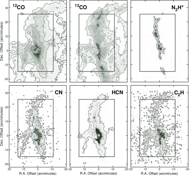
Fig. 1: Maps of the Orion Molecular Ridge obtained with 46^′′ –  60^′′ spatial resolution using the FCRAO (see Table 1). The peak integrated intensities ($\int\!T_{\rm mb}\>dv$), in K km s^-1 are: 700.00 (¹²CO), 89.41 (¹³CO), 30.13 (N₂H⁺), 69.42 (CN), 677.8 (HCN), 13.66 (C₂H). Contours superposed on the ¹³CO and C¹⁸O maps are in units of 0.10 of the peak value, with the peak contour shown being 0.9. Contours superposed on the N₂H⁺, CN, HCN, and C₂H maps are in units of 0.15 of the peak value. The rectangular region outlined in each map encompasses the region mapped in the H${}_{2}^{\>16}$O 1₁₀-1₀₁ 556.9 GHz transition by Herschel/HIFI. All map offsets are relative to $\alpha\,=\,$05^h35^m14${}^{\rm s}\!\!.$5, $\delta\>=\,-$05^o22^′37^′′ (J2000).

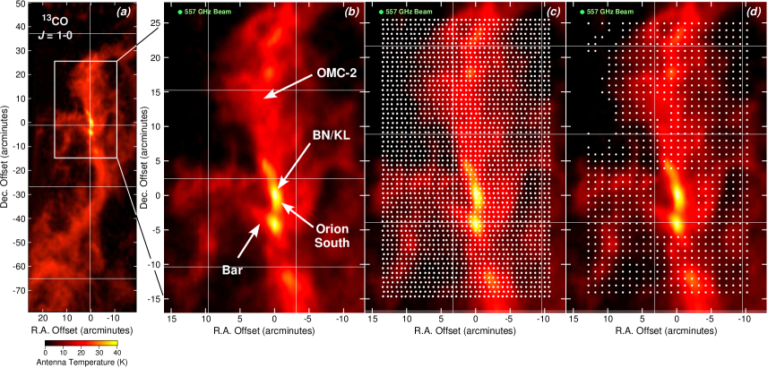
Fig. 2: Region mapped by Herschel/HIFI in this study. Panel (a): ¹³CO $J\!=\,$1 – 0 map of the Orion complex obtained with the Five College Radio Astronomical Observatory. The portion of Orion mapped here is enclosed within the white box. Panel (b): expanded view of the mapped region with important subregions denoted for reference. The size of the HIFI beam at 557 GHz is shown in green at the top. Panel (c): expanded view with the as-observed positions of the H₂O 1${}_{10}\,$– 1₀₁ 556.936 GHz and NH₃ $J,K=\;$1,0 – 0,0 572.498 GHz maps denoted with white dots. Panel (d): regridded positions on which all data were placed (see text). A total of 960 positions, separated by 1^′, were thus obtained; however, only data toward 834 positions are considered here, since some positions exhibited no detectable ¹³CO (or other) line emission, or because some lines of sight are dominated by outflow emission (e.g., near BN/KL and OMC-2) rather than quiescent gas emission. The regridded positions included in this study are denoted by white dots. All map offsets are relative to $\alpha\,=\,$05^h35^m14${}^{\rm s}\!\!.$5, $\delta\>=\,-$05^o22^′37^′′ (J2000).

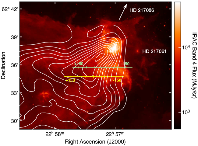
Fig. 3: Spitzer/IRAC Band 4 (7.87$\>\mu$m) image of Cepheus B with the contours of ¹²CO J = 3 – 2 emission obtained by Beuther et al. [2000] superposed. The northern and southern strip scans obtained by Herschel/HIFI in the 557 GHz H${}_{2}^{\>16}$O 1₁₀ – 1₀₁ and the 572 GHz NH₃ J,K$\,=\,$1,0 – 0,0 lines are also shown with offsets from the scan centers (see text) noted in arcseconds. The exciting stars, HD 217061 and HD 217086 (beyond the top edge of the image), are noted.

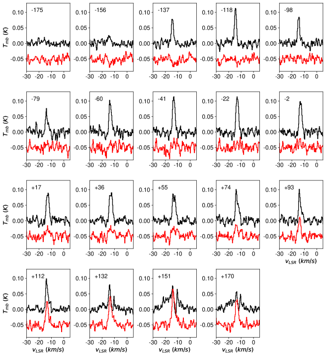
Fig. 4: Spectra of H₂O (black) and NH₃ (red) along the northern Cepheus B strip scan. The offsets, in arcseconds, relative to the (0,0) position of R.A. $=$ 22^h 57^m 16^s and Dec. $=+$62^o 35^′ 45^′′ (J2000) are given in the upper left of each panel.

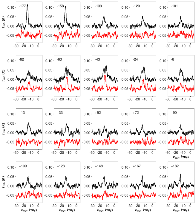
Fig. 5: Spectra of H₂O (black) and NH₃ (red) along the southern Cepheus B strip scan. The offsets, in arcseconds, relative to the (0,0) position of R.A. $=$ 22^h 57^m 24^s and Dec. $=+$62^o 34^′ 45^′′ (J2000) are given in the upper left of each panel.

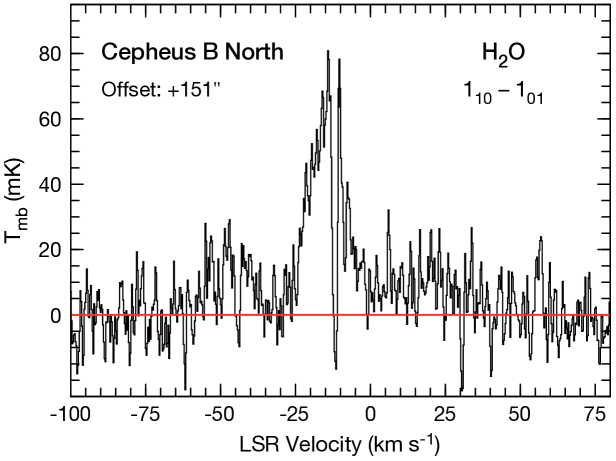
Fig. 6: Blowup of the continuum-subtracted H₂O spectrum along the Cepheus B northern strip scan showing evidence of an embedded outflow at RA $=$ 22^h 57^m 38^s and Dec. $=+$62^o 35^′ 45^′′ (J2000), corresponding to an offset of $+$ 151^′′ relative to the (0,0) position of R.A. $=$ 22^h 57^m 24^s and Dec. $=+$62^o 34^′ 45^′′ (J2000). The continuum-subtracted baseline is shown in red.

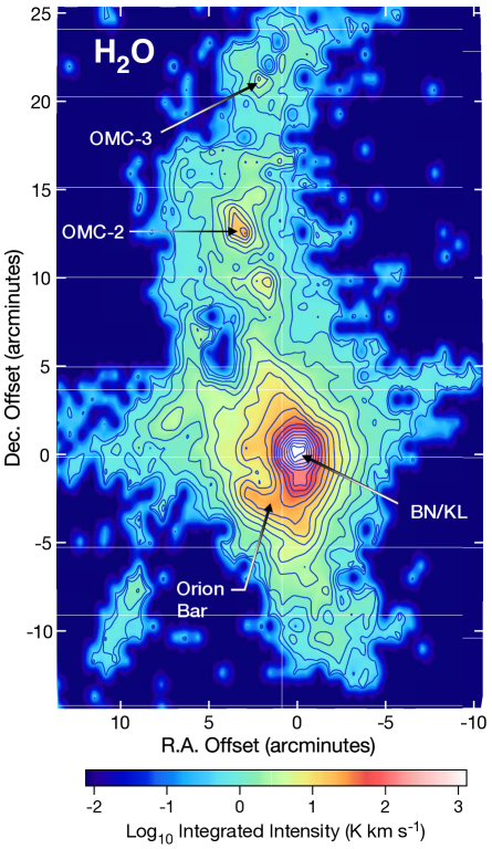
Fig. 7: Herschel/HIFI 556.936 GHz H₂O 1${}_{10}\,$– 1₀₁ integrated intensity map toward Orion. Note that, because of the large range of integrated intensities between the BN/KL region and the extended molecular ridge, the map is represented using a logarithmic scale. All map offsets are relative to $\alpha\,=\,$05^h35^m14${}^{\rm s}\!\!.$5, $\delta\>=\,-$05^o22^′37^′′ (J2000).

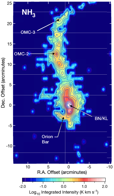
Fig. 8: Herschel/HIFI  572.498 GHz NH₃ $J$ $=\,$1 $\rightarrow$ 0 integrated intensity map toward Orion. Note that, because of the large range of integrated intensities between the BN/KL region and the extended molecular ridge, the map is represented using a logarithmic scale. All map offsets are relative to $\alpha\,=\,$05^h35^m14${}^{\rm s}\!\!.$5, $\delta\>=\,-$05^o22^′37^′′ (J2000).

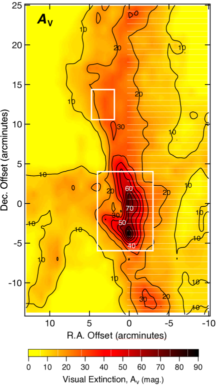
Fig. 9: Spatial distribution of visual extinction toward the Orion Molecular Ridge (see Section 3.1). The lower white box delineates the region containing BN/KL, the Orion Bar, and the low- and high-velocity outflows, while the upper white box delineates the region containing OMC-2. Both regions are excluded from the analysis presented here. All map offsets are relative to $\alpha\,=\,$05^h35^m14${}^{\rm s}\!\!.$5, $\delta\>=\,-$05^o22^′37^′′ (J2000).

Fig. 10: Spatial distribution of peak Orion ¹³CO optical depths based on the ¹²CO and ¹³CO measurements described in §2.1 and the analysis presented in §3.1.3. All map offsets are relative to $\alpha\,=\,$05^h35^m14${}^{\rm s}\!\!.$5, $\delta\>=\,-$05^o22^′37^′′ (J2000).

Fig. 11: Percentage of the 898 Orion ¹³CO map positions within the water map area with peak ¹³CO optical depths greater than the $x$-axis value. The median peak ¹³CO optical depth is 0.27 and more than 95% of the peak ¹³CO optical depths are less than 0.69.

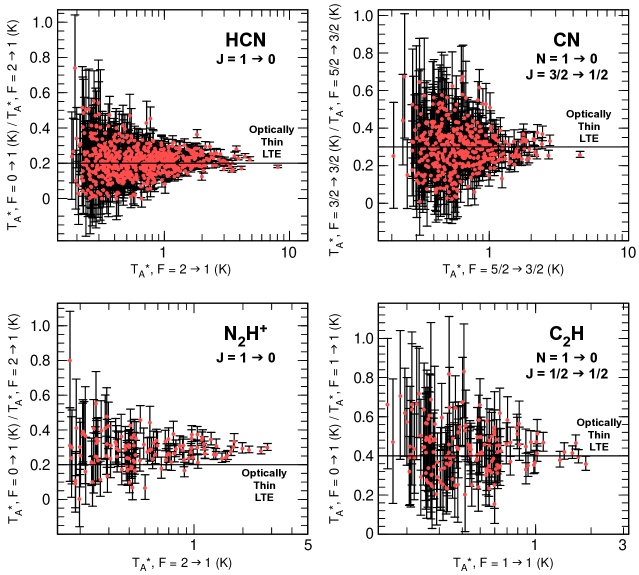
Fig. 12: Hyperfine intensity ratios toward Orion for HCN, CN, N₂H⁺, and C₂H showing, in each panel, the ratio of the weakest hyperfine component to the strongest. Such ratios are most sensitive to the optical depth for each species. Also shown are the ratios expected for optically thin LTE emission. Although there is scatter and uncertainty in the ratio for the weaker intensity lines, as the lines become stronger, the ratio approaches the LTE optically thin value. The slightly larger-than-LTE value for N₂H⁺ is discussed in the text.

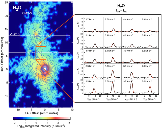
Fig. 13: H₂O spectra obtained toward a portion of the Orion Ridge indicated by the boxed region on the left. Each spectrum was fitted with a single Gaussian line, in red, whose FWHM is given in the upper left of each panel. In every case, a Gaussian profile provides an excellent fit to the data. This suggests that no significant frequency redistribution of escaping H₂O photons is occurring, which would result in a notable reduction of emission at line center and an enhancement of emission in the line wings.

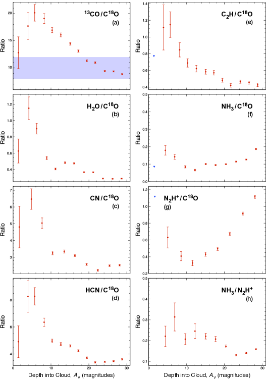
Fig. 14: Plots of the ratios of the integrated intensities of the Herschel- and FCRAO-observed species versus depth into the Orion Molecular Ridge, measured in visual magnitudes, determined from the measured ¹³CO column densities and the relations given in Eqns. (1) and (2). For clarity of presentation, the number of data points per plot has been reduced from 636 data points (for 0$\,\leq\,$A_V$\,\leq\,$30) by averaging all data with a signal-to-noise ratio $\geq\>$3 within bins of A_V. The error bars for each point represent the error-weighted mean and 1$\sigma$ uncertainty in the mean for the co-averaged points in each bin. The purple region in panel (a) indicates the ¹³CO / C¹⁸O ratio range expected deep within the Ridge based on the ¹³C and ¹⁸O relative abundances measured toward Orion (see text).

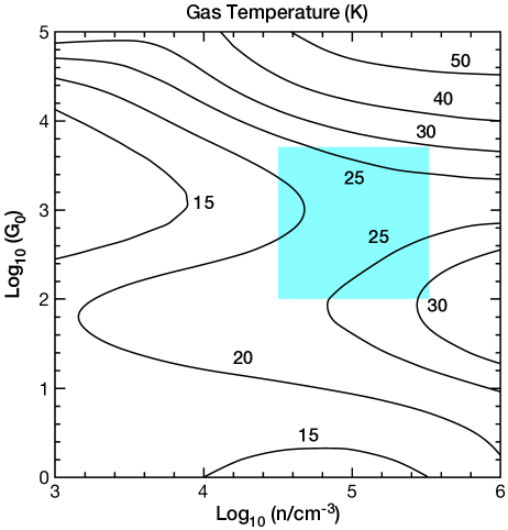
Fig. 15: Average gas temperature within the region of peak water abundance (after Hollenbach et al. [2009]). The blue box, which has been added, shows the range of densities, $n$($=n_{\rm H}+$2$n_{H_{2}}$), and FUV field strengths, $G_{\rm o}$, appropriate to the Orion Molecular Ridge. The average values for the Ridge are $n\>\sim\,$10⁵ cm^-3 and $G_{\rm o}$$\,\sim\>$500.

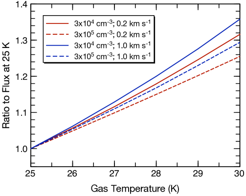
Fig. 16: Ratio of the H₂O 1${}_{10}\,$– 1₀₁ 557 GHz line flux calculated for a range of gas temperatures relative to that at 25 K. H₂ densities of 3$\,\times\,$10${}^{4}\>$cm^-3 (solid lines) and 3$\,\times\,$10${}^{5}\>$cm^-3 (dashed lines) and line widths per A_V bin of 0.2 km s^-1 (red lines) and 1.0 km s^-1 (blue lines) are assumed. An H₂ column density per A_V bin of 2.4$\,\times\,$10${}^{21}\>$cm^-2 is assumed, corresponding to an A_V bin width of 2.5 magnitudes, and an H₂O abundance of 10^-7. (Note: The line flux ratios vary by less than 20 percent with a factor of 10 reduction in the assumed H₂O abundance.)

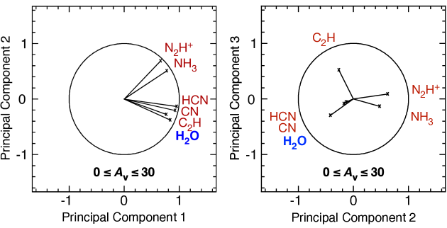
Fig. 17: Results of the Principal Component Analysis for H₂O, C₂H, CN, HCN, NH₃, and N₂H⁺ for 820 Orion Molecular Ridge positions possessing cloud depths between A_V$\,=\,$0 and 30. Principal Components 1 and 2 capture a cumulative fraction of 87% of the total variance while Principal Components 2 – 3 capture 94% of the total variance. Clearly, gas-phase H₂O is strongly correlated with HCN, CN, and C₂H while H₂O is largely uncorrelated with NH₃ and N₂H⁺, species that are expected to have their peak abundance deep within dense clouds.

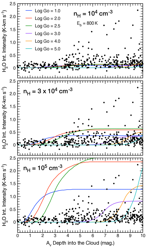
Fig. 18: Plots showing the gas-phase-H₂O integrated intensity versus A_V for the 834 positions along the Orion Ridge (see caption to Fig. 2). Superposed on each panel are the model-predicted H₂O integrated intensities for an atomic oxygen-to-dust grain binding energy of 800 K [Tielens & Hagen, 1982] and various values of $G_{\rm o}$ and gas densities of 10⁴ cm^-3 (top panel), 3$\,\times\,$10⁴ cm^-3 (middle panel), and 10⁵ cm^-3 (bottom panel).

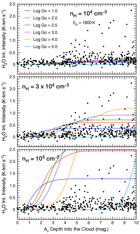
Fig. 19: Plots showing the gas-phase-H₂O integrated intensity versus A_V for the 834 positions along the Orion Ridge (see caption to Fig. 2). Superposed on each panel are the model-predicted H₂O integrated intensities for an atomic oxygen-to-dust grain binding energy of 1800 K [He et al., 2015] and various values of $G_{\rm o}$ and gas densities of 10⁴ cm^-3 (top panel), 3$\,\times\,$10⁴ cm^-3 (middle panel), and 10⁵ cm^-3 (bottom panel).

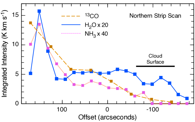
Fig. 20: Integrated intensity of ¹³CO, H₂O, and NH₃ as a function of offset from the Cepheus B northern strip scan (0,0) position, i.e., R.A. 22^h 57^m 16^s, Dec. $+$62^o 35^′ 45^′′ (J2000). The ¹³CO strip scan was obtained using FCRAO, while the H₂O and NH₃ strip scans were obtained using Herschel. In order to better illustrate the trends, the H₂O integrated intensities have been multiplied by 20, and the NH₃ integrated intensities have been multiplied by 40.

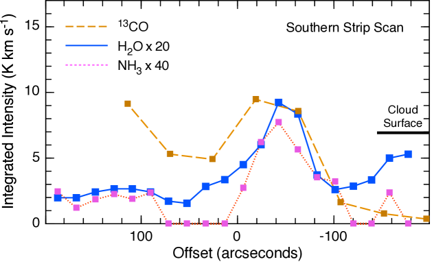
Fig. 21: Integrated intensity of ¹³CO, H₂O, and NH₃ as a function of offset from the Cepheus B southern strip scan (0,0) position, i.e., R.A. 22^h 57^m 24^s, Dec. $+$62^o 34^′ 45^′′ (J2000). The ¹³CO strip scan was obtained using FCRAO, while the H₂O and NH₃ strip scans were obtained using Herschel. In order to better illustrate the trends, the H₂O integrated intensities have been multiplied by 20, and the NH₃ integrated intensities have been multiplied by 40.

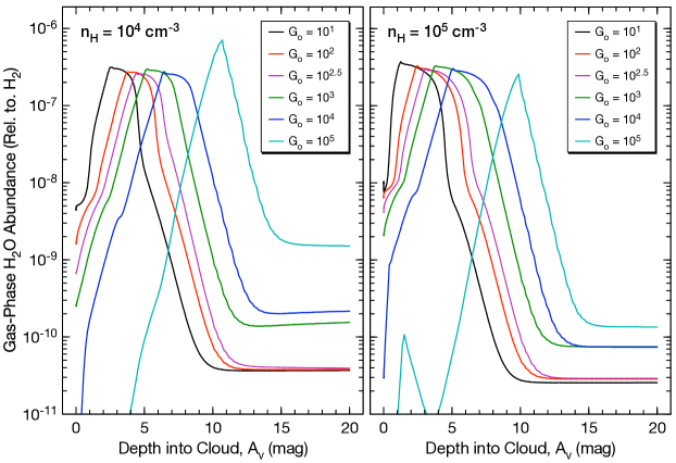
Fig. 22: Predicted gas-phase H₂O abundance vs. depth into clouds, measured in magnitudes of visual extinction, A_V, and FUV flux, $G_{\rm o}$, for clouds of gas density 10⁴ cm^-3 and 10⁵ cm^-3. An atomic oxygen binding energy of 1800 K is assumed (see text).

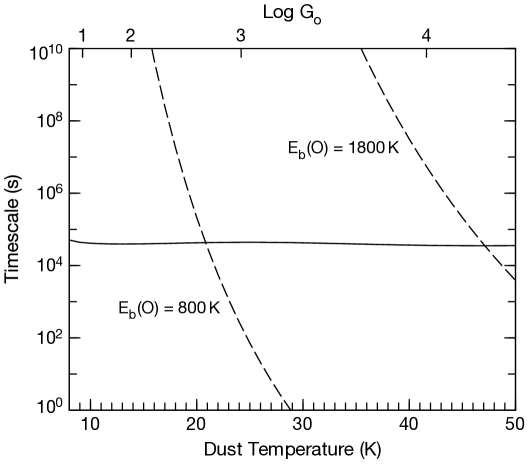
Fig. 23: Timescales relevant to OH formation on grains. The dashed curves show the timescale for thermal desorption of an O atom on a grain for both the old (800 K) and new (1800 K) value of the O binding energy. The solid curve is the timescale for formation of an OH molecule given an O atom adsorbed to the surface, which is dominated by the time it takes for an H atom to arrive on the grain surface (see text). The relation between the dust grain temperature and $G_{\rm o}$ is that provided in Hollenbach et al. [2009]. Once the H atom has adsorbed onto the surface, its diffusion is so rapid that the reaction with O is essentially instantaneous (compared to the H-accretion timescale). At dust temperatures where the solid line is below the dashed line, O atoms remain on grain surfaces sufficiently long to combine with an H atom to form OH (and, ultimately, H₂O).

References

- [1]
- Aikawa et al. [2012] Aikawa, Y., Kamuro, D., Sakon, I., et al. 2012, A&A, 538, A57
- Allen et al. [2012] Allen, T.S., Gutermuth, R.A., Kryukova, E., et al. 2012, Ap. J., 750, 125
- Bally et al. [1987] Bally, J., Langer, W. D., Stark, A. A., et al. 1987, Ap. J., 312, L45
- Bergin et al. [1994] Bergin, E. A., Goldsmith, P. F., Snell, R. L., et al. 1994, Ap. J., 431, 674
- Bergin et al. [2000] Bergin, E. A., Melnick, G. J., Stauffer, J.R., et al. 2000, Ap. J., 539, L132
- Bergin et al. [1996] Bergin, E. A., Snell, R. L., & Goldsmith, P. F. 1996, Ap. J., 460, 343
- Beuther et al. [2000] Beuther, H., Kramer, C., Deiss, B., et al. 2000, A&A, 362, 1109
- Bisbas et al. [2012] Bisbas, T.G., Bell, T.A., Viti, S., et al. 2012, M.N.R.A.S., 427, 2100
- Boogert, Gerakines, & Whittet [2015] Boogert, A.C.A., Gerakines, P.A., & Whittet, D.C.B. 2015, A.R.A.&A., 53, 541
- Caselli et al. [2012] Caselli, P., Keto, E., Bergin, E.A., et al. 2012, Ap. J., 759, L37
- Cernicharo et al. [2006] Cernicharo, J., Goicoechea, J.R., Pardo, J.R., et al. 2006, Ap. J., 642, 940
- Chen et al. [2014] Chen, J.-H., Goldsmith, P.F., Viti, S., et al. 2014, Ap. J., 793, 111
- Coutens et al. [2012] Coutens, A., Vastel, C., Caux, E., et al. 2012, A&A, 539, A132
- Danby et al. [1988] Danby, G., Flower, D.R., Valiron, P., et al. 1988, M.N.R.A.S., 235, 229
- Daniel, Dubernet, & Grosjean [2011] Daniel, F., Dubernet, M., & Grosjean, A. 2011, A&A, 536, A76
- Daniel et al. [2005] Daniel, F., Dubernet, M.-L., Meuwly, M., et al. 2005, M.N.R.A.S., 363, 1083
- Dubernet et al. [2009] Dubernet, M.-L., Daniel, F., Grosjean, A. et al. 2009, A&A, 497, 911
- Dumouchel, Faure, & Lique [2010] Dumouchel, F., Faure, A., & Lique, F. 2010, M.N.R.A.S., 406, 2488
- Dutrey et al. [1991] Dutrey, A., Langer, W. D., Bally, J., et al. 1991, A&A, 247, L9
- Fraser et al. [2001] Fraser, H.J., Collings, M.P., McCoustra, M.R.S., et al. 2001, M.N.R.A.S., 327, 1165
- Gibb et al. [2004] Gibb, E.L., Whittet, D.C.B., Boogert, A.C.A., et al. 2004, Ap. J. Suppl., 151, 35
- Goldsmith et al. [2011] Goldsmith, P.F., Liseau, R., Bell, T., et al. 2011, Ap. J., 737, 96
- Habing [1968] Habing, H. J. 1968, Bull. Astron. Inst. Netherlands, 19, 421
- Hawkins & Jura [1987] Hawkins, I., & Jura, M. 1987, Ap. J., 317, 926
- He et al. [2015] He, J., Shi, J., Hopkins, T., et al. 2015, Ap. J., 801, 120
- Hollenbach et al. [2009] Hollenbach, D.J., Kaufman, M. J., Bergin, E.A., et al. 2009, Ap. J., 690, 1497
- Jensen et al. [2000] Jensen, M.J., Bilodeau, R.C., Safvan, C.P., et al. 2000, Ap. J., 543, 764
- Johnstone & Bally [1999] Johnstone, D., & Bally, J. 1999, Ap. J., 510, L49
- Kainulainen, Lehtinen, & Harju [2006] Kainulainen, J., Lehtinen, K. & Harju, J. 2006, A&A, 447, 597
- Kester, Higgins & Teyssier [2017] Kester, D., Higgins, R. & Teyssier, D. 2017, A&A, 599, 115
- Keto, Rawlings & Caselli [2014] Keto, E., Rawlings, J. & Caselli, P. 2014, M.N.R.A.S., 440, 2616
- Keto & Rybicki [2010] Keto, E., & Rybicki, G. 2010, Ap. J., 716, 1315
- Kristensen & van Dishoeck [2011] Kristensen, L. E. & van Dishoeck 2011, Astron. Nachr., 332, No. 5, 475
- Kristensen et al. [2011] Kristensen, L. E, van Dishoeck, Tafalla, M., et al. 2011, A&A, 531, L1
- Kryukova et al. [2012] Kryukova, E., Megeath, S. T., Gutermuth, R. A., et al. 2012, A. J., 144, 31
- Langer & Penzias [1990] Langer,W. D., & Penzias, A. A. 1990, Ap. J., 357, 477
- Larsson et al. [2007] Larsson, B., Liseau, R., Pagani, L., et al. 2007, A&A, 466, 999
- Lee et al. [2014] Lee, S., Lee, J.-E., Bergin, E.A., et al. 2014, Ap. J. Suppl., 213, 33
- Lique et al. [2010] Lique, F., Spielfiedel, A., Feautrier, N., et al. 2010, J. Chem. Phys., 132, 024303
- Liseau et al. [2012] Liseau, R., Goldsmith, P.F., Larsson, B., et al. 2012, A&A, 541, 73
- Loughnane et al. [2012] Loughnane, R. M., Redman, M. P., Thompson, M. A., et al. 2012, M.N.R.A.S., 420, 1367
- Melnick & Kaufman [2015] Melnick, G.J., & Kaufman, M.J. 2015, Ap. J., 806, 227
- Melnick et al. [2011] Melnick, G. J., Tolls, V., Snell, R. L., et al. 2011, Ap. J., 727, 13
- Minchin, Ward-Thompson, & White [1992] Minchin, N. R., Ward-Thompson, D., & White, G. J. 1992, A&A, 265, 733
- Mookerjea et al. [2006] Mookerjea, B., Kramer, C., Röllig, M., et al. 2006, A&A, 456, 235
- Mottram et al. [2013] Mottram, J.C., van Dishoeck, E.F., Schmalz, M., et al. 2013, A&A, 558, A126
- Mueller et al. [2014] Mueller, M., Jellema, W., Olberg, M. et al. “The HIFI Beam: Release #1 Release Note for Astronomers,” ESA Doc.: HIFI-ICC-RP-2014-001, v1.1, 1 Oct 2014
- Mullins et al. [2016] Mullins, A.M., Loughnane, R.M., Redman, M.P., et al. 2016, M.N.R.A.S., 459, 2882
- Neufeld et al. [2007] Neufeld, D. A., Hollenbach, D. J., Kaufman, M. J., et al. 2007, Ap. J., 664, 890
- Noble et al. [2013] Noble, J. A., Fraser, H. J., Aikawa, Y., et al. 2013, Ap. J., 775, 85
- Ott [2010] Ott, S. 2010, Astronomical Data Analysis Software and Systems XIX, 434, 139
- Pabst et al. [2019] Pabst, C. H. M., Goicoechea, D., Teyssier, et al. 2019, in preparation
- Pety et al. [2017] Pety, J., Guzmán, V. V., Orkisz, J. H., et al. 2017, A&A, 599, 98
- Pirogov [1999] Pirogov, L., 1999, A&A, 348, 600
- Pirogov et al. [2003] Pirogov, L., Zinchenko, I., Caselli, P., et al. 2003, A&A, 405, 639
- Reid et al. [2009] Reid, M.J., Menten, K.M., Zheng, X.W., et al. 2009, Ap. J., 700, 137
- Ripple et al. [2013] Ripple, F., Heyer, M.H., Gutermuth, R., et al. 2013, M.N.R.A.S., 431, 1296
- Roelfsema et al. [2012] Roelfsema, P. R., Helmich, F. P., Teyssier, D., et al. 2012, A&A, 537, A17
- Röllig et al. [2007] Röllig, M., Abel, N. P., Bell, T. et al. 2007, A&A, 467, 187
- Savage et al. [2002] Savage, C., Apponi, A.J., Ziurys, L.M., et al. 2002, Ap. J., 578, 211
- Schilke et al. [1992] Schilke, P., Walmsley, C.M., Pineau Des Forêts, G., et al. 1992, A&A, 256, 595
- Schmalzl et al. [2014] Schmalzl, M., Visser, R., Walsh, C., et al. 2014, A&A, 572, A81
- Snell et al. [2000] Snell, R. L., Howe, J. E., Ashby, M. L. N., et al. 2000, Ap. J., 539, L93
- Spielfiedel et al. [2012] Spielfiedel A., Feautrier N., Najar F., et al. 2012, M.N.R.A.S., 421, 1891
- Stacey et al. [1993] Stacey, G.J., Jaffe, D.T., Geis, N., et al. 1993, Ap. J., 404, 219
- Tatematsu et al. [1993] Tatematsu, K., Umemoto, T., Murata, Y., et al. 1993, Ap. J., 404, 643
- Tielens & Hagen [1982] Tielens, A. A., & Hagen, W. 1982, A&A, 114, 245
- Ungerechts et al. [1997] Ungerechts, H., Bergin, E. A., Goldsmith, P. F., et al. 1997, Ap. J., 482, 245
- van der Tak et al. [2007] van der Tak, F. F. S., Black, J.H., Schöier, F.L. et al. 2007, A&A, 468, 627
- Womack et al. [1992] Womack, M., Ziurys, L.M., Wyckoff, S., et al. 1992, Ap. J., 387, 417
- Yang et al. [2010] Yang, B., Stancil, P.C., Balakrishnan, N., et al. 2010, Ap. J., 718, 1062