Gravastars in $f(R,T,R_{\mu\nu}T^{\mu\nu})$ Gravity

Abstract

This work is devoted to study the analytical and regular solutions of a particular self-gravitating object (i.e., gravastar) in a particular theory of gravity. We derive the corresponding field equations in the presence of effective energy momentum tensor associated with the perfect fluid configuration of a spherical system. We then describe the mathematical formulations of the three respective regions i.e., inner, shell and exterior of a gravastar separately. Additionally, the significance and physical characteristics along with the graphical representation of gravastars are discussed in detail. It is seen that under some specific constraints, $f(R,T,R_{\mu\nu}T^{\mu\nu})$ gravity is likely to host gravastars.

Keywords: Gravitation, Cylindrically symmetric spacetime, Isotropic pressure.

1 Introduction

General relativity (GR) laid down the foundation of new era of mathematical physics that has led to the discovery of the new ideas in the field of astrophysics, cosmology, etc. Einstein came up with the notion of matter-geometry relationship that led him to explain the concept of gravity in terms of curvature in spacetime. There are some surprising and revolutionary results based on some notable observations, like cosmic microwave background radiation, type Ia supernovae, etc., [1]-[3] suggested the accelerated expansion of our universe. Modified theories of gravity are among the most popular approaches considered for the explanation of the structure and origins of the universe. Furthermore, the modification of GR may lead us to explain the history and the accelerated expansion of the universe, and the role of dark matter in a better way. Nojiri and Odinstov [4] reformulated the Hilbert action by considering the generic function of Ricci scalar i.e., $f(R)$ in place of $R$, thereby opening a arena for modified theories of gravity. Afterwards, many facts and unsorted problems about the structure of different stellar objects and mystery of universe were discussed [5]-[17].

The generalization of $f(R)$ was unveiled by Harko et al. [18] named as $f(R,T)$ in where $T$ is the trace of energy momentum tensor. The motivation of including $T$ in $f(R)$ is that it may give us viable results with respect to quantum gravity by retaining coupling between matter and geometry. They considered some definite forms of the function $f(R,T)$ and evaluated the corresponding field as well as conservation equations. Moreover, they examined the scalar field model in detail. In order to do so, they acknowledged the cosmological significance of $f(R,T^{\phi})$ model. Furthermore, they demonstrated the equation of motion of test particle and the Newtonian limit of equation of motion.

Likewise, to acquire information on how the strong non-minimal coupling of matter and geometry influenced the results of $f(R,T)$ theory, the generalization in this theory has been developed. Subsequently, Haghani et al. [19] introduced the $f(R,T,Q)$ theory ($Q\equiv R_{\mu\nu}T^{\mu\nu}$) which involves the contraction of the Ricci scalar with the stress energy momentum tensor. They deduced the field equations for the motion of test particle in the $f(R,T,Q)$ gravity for both the conservative and non-conservative cases. They claimed that this theory is non-conserved because of the extra force acting on the particles. The Dolgov-Kawasaki instability is also examined along with the stability condition. In addition to this, some cosmological applications were studied, analytically and numerically by Ayuso et al. [20]. Odintsov and Sáez-Gómez [21] demonstrated the phenomenology of the $f(R,T,Q)$ gravity and analyzed the instability in this gravity. Baffou et al. [22] explored the model in $f(R,T,Q)$ gravity to discuss the stability utilizing the de-Sitter and power law solutions. They also evaluated the generalized Friedmann equations. The $f(R,T,Q)$ gravity enforced to look upon the universe extensively. Dvali [23] explained thoroughly some of the properties of the theories that can reformulate gravity. Yousaf et al. [24]-[26] studied the phenomena of dynamical instability in $f(R,T,Q)$ gravity by taking into account different interior geometries. They used a specific Harrison-Wheeler equation of state in order to describe stable regions of the corresponding stellar structures. Furthermore, Yousaf et al. [27] calculated junction condition in order to match exterior Einstein-Rosen bridge with an interior cylindrical spacetime.

Existence of a new hypothetical star can be evident as a consequence of a gravitational collapse. It can be attained by scrutinizing the basic concept of Bose-Einstein condensation (BEC). In BEC, the gas of bosons are cooled to the temperature where the molecules loses infinite kinetic energy. One can recognize that all the molecules of bosons are indistinguishable having same quantum spin, thereby not following Pauli exclusive principle. Here, the molecules continue to move slowly so that they must obey the uncertainty principle. The one of the final states of gravitational collapse could give rise to gravastar, thereby indicating this as an alternative to black hole as suggested by [28]. Such kind of structure is mainly comprised of three regions, namely, inner region, shell and exterior region. The inner region is supplemented by that matter in which the energy density $\rho$ is equal to the negative pressure $P$ i.e., $\rho=-P$. This state is the main hinderance that doed not permit gravastar to form singularity. The presence of dark energy in the inner region is a source of repulsive force that is exerting on the shell. The shell contains the effective matter incorporate with the perfect fluid. In this region, the energy density $\rho$ is equal to the pressure $P$ of the relativistic fluid, i.e., $\rho=P$. The shell in return apply force on the inner region so that the gravastar would remain in the hydrostatic equilibrium. The exterior region is entirely vacuum. It is an indication of the negligible atmospheric pressure out there. So the EoS $\rho=P=0$ is adopted for this region. One can see the formation of naked singularity and black holes phenomenon with the help of mathematical equation presented by Virbhadra et al. [29], [30]. Gravitational collapse as well as the stability of self-gravitating systems have also been analyzed in literature [31]-[34].

Mazur and Mottola [28] presented the visualization of the gravastar and claimed the absence of event horizon and singularity in such structures. They also discussed the thermodynamic stability of the gravastar. Later Visser and David [35] extended the work of Mazur and Mottola and examined the stability of this star by taking into account the physical characteristics and equation of state. Cattoen et al. [36] used the concept that if there does not exist any shell in the composition of gravastar then it must have anisotropic pressure. Chirenti and Rezzolla [37] demonstrated the stability of a gravastar against the generic perturbation scheme. Additionally, gravastar can be distinguished from the black hole of same mass as their quasi-normal modes are different. Bilić et al. [38] formulated some solutions of gravastar through Born infeld Phantom background. Horvat et al. [39] performed stability analysis for the static spherically symmetric gravastars and observed that anisotropic gravastar structures exhibiting continuous pressure are radially stable.

Sakai et al. [40] examined the optical images of gravastar composed of unstable circular orbit. In fact, they assumed two optical sources and described both of them in detail. Chirenti et al. [41] worked on the ergoregion instability in a rotating gravastar and declared it to be unstable. Rahaman et al. [42] studied the role of electric charge on gravastar with (2+1)-dimensional metric. They studied some theoretical results for the stability of spherical gravastars. Pani et al. [43] constructed non-rotating gravastar models after matching smoothly Schwarzschild and de Sitter spacetimes.

Ghosh et al. [44] analyzed the existence of these structures by taking higher dimensional geometries. Das et al. [45] extended the concept of gravastars $f(R,T)$ gravity and checked some important characteristics about their theoretical existence. Shamir and Mushtaq [46] modified their analysis for $f(G,T)$ gravity. Yousaf [47, 48] found some mathematical models of compact objects in $f(G,T)$ gravity through structure scalars. Yousaf et al. [49] analyzed the effects of electromagnetic field on the possible formation of gravastars in $f(R,T)$ gravity. Bhatti and his collaborators [50], [51] extended these results for spherically and cylindrically symmetric spacetime in GR. Sharif and Waseem [52] described the modeling of gravastars with the help of conformal motion. Recently, Yousaf [53] found non-singular solutions of gravastars in $f(R,T)$ gravity by taking static cylindrically symmetric spacetime. He found the existence of cylindrical gravastar-like structures in $f(R,T)$ gravity.

The present work is devoted to study the formation of gravastars for the isotropic self-gravitating spherical system in $f(R,T,Q)$ theory. In the next section the field as well as the basic equation for $f(R,T,Q)$ theory have been derived. The construction of gravastars including the detailed discussion about the modeling of all the three regions of gravastars are discussed in section 3. In section 4, the appropriate junction conditions are calculated, while the section 5 is devoted to describe various physical characteristics of the gravastar in $f(R,T,Q)$ theory along with their graphical representation. Finally in section 6, we sum up all the results.

2 $f(R,T,Q)$ Theory of Gravity

The motivation to adopt $f(R,T,Q)$ theory is that in these type of theories the more generalized form of the matter Lagrangian $L_{m}$ has been used describing the strong non-minimal coupling between the matter and geometry contrary to the $f(R,T)$ theory. For instance, $f(R,T,Q)$ can be generalized by the addition of the term $Q\equiv R_{\mu\nu}T^{\mu\nu}$ in the Lagrangian. Einstein Born Infeld theories are the example of such coupling. The thought-provoking distinction between the $f(R,T,Q)$ and $f(R,T)$ theories is that even if we consider the traceless energy momentum tensor i.e., $T=0$ in $f(R,T,Q)$, this theory will be able to explain about the non-minimal coupling to the electromagnetic field due to the addition of term $R_{\mu\nu}T^{\mu\nu}$ in the Lagrangian.

The $f(R,T,Q)$ theories can explain the late time acceleration without using the approach of the cosmological constant or dark energy. In contrast with the $f(R,T)$ theories, these theories involve the effects of the extra force exerted on the massive particle even if we consider $L_{m}=-\rho$, where $\rho$ is the energy density of the relativistic fluid. The characteristics of galactic rotation curves could be explained in the presence of this extra force without considering the hypothesis of dark matter. Hence, the complex modified equations are attained in this theory. One can achieve the various qualitative cosmological solutions with different forms of function in the $f(R,T,Q)$ theories. This theory makes feasible for us to reveal about the evolution in the universe at the early stages instead of using the inflationary paradigm, which is quite challenging.

Odintsov and Sáez-Gómez [21] demonstrated that the finest power law version of $f(R,T,Q)$ theories might be represented by the Horava-like gravity power-counting renormalizable covariant gravity. The action integral for the case of $f(R,T,Q)$ theory can be stated as

$$S=\frac{1}{2}\left(\int d^{4}xf(R,T,R_{\alpha\beta}T^{\alpha\beta})\sqrt{-g}+\int d^{4}xL_{m}\sqrt{-g}\right),$$ (1)

where $R$ is the Ricci scalar, $Q\equiv R_{\alpha\beta}T^{\alpha\beta}$, $L_{m}$ is the matter Lagrangian, $T$ and $g$ are the traces of energy momentum and metric tensors, respectively. By varying the above action respecting $g_{\mu\nu}$, one can get

$$- G_{\alpha\beta}(f_{Q}L_{m}-f_{R})-g_{\alpha\beta}\left\{\frac{f}{2}-\Box f_{R}-\frac{R}{2}f_{R}-\frac{1}{2}\nabla_{\pi}\nabla_{\rho}(f_{Q}T^{\pi\rho})-L_{m}f_{T}\right\}$$ (2)

$$+ 2f_{Q}R_{\pi(\alpha}T_{\beta)}^{\pi}+\frac{1}{2}\Box(f_{Q}T_{\alpha\beta})-\nabla_{\pi}\nabla_{(\alpha}[T_{\beta)}f_{Q}]-2(f_{T}g^{\pi\rho}+f_{Q}R^{\pi\rho})\frac{\partial^{2}L_{m}}{\partial g^{\alpha\beta}\partial g^{\pi\rho}}$$

$$- T_{\alpha\beta}^{(m)}(f_{T}+\frac{R}{2}f_{Q}+1)-\nabla_{\alpha}\nabla_{\beta}f_{R}=0,$$

where $\nabla_{\alpha}$ is a covariant derivative, $\Box=g^{\alpha\beta}\nabla_{\alpha}\nabla_{\beta}$, $G_{\lambda\sigma}$ is an Einstein tensor and $T_{\lambda\sigma}$ describes energy-momentum tensor that can be described as follows

$$T_{\lambda\sigma}^{(m)}=-\frac{2}{\sqrt{-g}}\frac{\delta(\sqrt{-g}\textit{L}_{m})}{\delta{g^{\lambda\sigma}}}.$$ (3)

Here, the subscripts $R,~{}T$ and $Q$ indicate the partial derivative of $f$ with respect to its arguments. From Eq.(3), one can write

$$3\Box f_{R}+\frac{1}{2}\Box(f_{Q}T)-T(f_{T}+1)+\nabla_{\pi}\nabla_{\rho}(f_{Q}T^{\pi\rho})+R(f_{R}-\frac{T}{2}f_{Q})$$

$$+(Rf_{Q}+4f_{T})\textit{L}_{m}-2f+2R_{\pi\rho}T^{\pi\rho}f_{Q}-2\frac{\partial^{2}\textit{L}_{m}}{\partial g^{\lambda\sigma}\partial g^{\pi\rho}}\left(f_{T}g^{\pi\rho}+f_{Q}R^{\pi\rho}\right).$$

By applying the conditions of vacuum case on the field equation of $f(R,T,Q)$ theory, equations of motion for $f(R)$ theory can be retrieved. Nonetheless, the case $Q=0$ provides the dynamics of $f(R,T)$ theory. It is important to stress that the value of the last term will be non-zero, if $\textit{L}_{m}$ contains second or higher order terms. However, by setting a particular choice of $L_{m}$, one can ignore this last term from the calculations. The $f(R,T,Q)$ theory is an un-conserved theory which eventually leads an extra force (even within our assumed case $L_{m}=-\rho$). Our present theory is a special form of gravitational theory. The non-minimal coupling between matter and geometry can be dissolved in $f(R,T)$ gravity, when one consider a charged gravitating sources in the analysis. This would boils down $f(R,T)$ equation of motion to that of $f(R)$. However, in this theory, the term $Q$ preserves such non-minimal coupling of gravity with the relativistic fluid. One can write Eq.(2) in the following alternative form as

$$G_{\nu}^{\mu}=T_{\nu}^{\mu(eff)},$$ (4)

where

$$T_{\mu\nu}^{(eff)} = \frac{1}{f_{R}-L_{m}f_{Q}}\left[\left(f_{T}+\frac{1}{2}Rf_{Q}+1\right)T_{\mu\nu}^{(m)}+\left\{\right.\frac{f}{2}-\frac{f_{R}R}{2}-L_{m}f_{T}\right.$$ (5)

$$- \frac{1}{2}\nabla_{\alpha}\nabla_{\beta}(f_{Q}T^{\alpha\beta})\left.\right\}g_{\mu\nu}-\frac{1}{2}\Box(f_{Q}T_{\mu\nu})-(g_{\mu\nu}g^{\alpha\beta}\nabla_{\alpha}\nabla_{\beta}-\nabla_{\mu}\nabla\nu)f_{R}$$

$$- 2f_{Q}R_{\alpha(\mu}T_{\nu)}^{\alpha}+\nabla_{\alpha}\nabla_{(\mu}[T_{\nu)}^{\alpha}f_{Q}\left.\right]+\left.2(f_{Q}R^{\alpha\beta}+f_{T}g^{\alpha\beta})\frac{\partial^{2}L_{m}}{\partial g^{\mu\nu}\partial g^{\alpha\beta}}\right],$$

could be regarded as an effective energy-momentum tensor for $f(R,T,Q)$ gravity. The purpose of the present paper is to analyze the effects of $f(R,T,Q)$ terms on the stability of gravastars. For this purpose, we consider an isotropic matter distribution having the following form

$$T_{\mu\nu}^{(m)} =(\rho+P)u_{\mu}u_{\nu}-Pg_{\mu\nu},$$ (6)

where $u^{\mu}$ is the four velocity of the fluid and $P$ stands for the fluid’s pressure.

3 Formation of Static Spherically Symmetric Gravastars in $f(R,T,Q)$ Gravity

Now, we must assume a static irrotational spherically symmetric spacetime, which in Schwarzschild-like coordinate system, can be expressed as

$$ds^{2}=e^{\nu(r)}dt^{2}-e^{\mu(r)}dr^{2}-r^{2}(d\theta^{2}+\sin^{2}\theta d\phi^{2}).$$ (7)

The non-zero components of Einstein tensor for the spherically symmetric spacetime are found as follows

$$G_{0}^{0} = \frac{e^{-\lambda}}{r^{2}}(-1+e^{\lambda}+\lambda^{\prime}r),$$ (8)

$$G_{1}^{1} = \frac{e^{-\lambda}}{r^{2}}(-1+e^{\lambda}-\nu^{\prime}r),$$ (9)

$$G_{2}^{2}=G_{3}^{3} = \frac{e^{-\lambda}}{4r}\left[2(\lambda^{\prime}-\nu^{\prime})-(2\nu^{\prime\prime}+\nu^{\prime 2}-\nu^{\prime}\lambda^{\prime})r\right],$$ (10)

where prime denotes derivatives with respect to $r$. The modified field equations can be found after using Eqs.(4), (5), (6), (7), (8), (9) and (10) as

$$\frac{e^{-\lambda}}{r^{2}}\left(-1+e^{\lambda}+\lambda^{\prime}r\right)=\frac{1}{f_{R}+\rho f_{Q}}\left[\right.\rho\chi_{1}+\rho^{\prime}\chi_{2}+\frac{\rho^{\prime\prime}f_{Q}e^{-\lambda}}{2}+P\chi_{3}$$

$$+P^{\prime}\chi_{4}-\frac{P^{\prime\prime}f_{Q}e^{-\lambda}}{2}+D_{0}\left.\right],$$ (11)

$$\frac{e^{-\lambda}}{r^{2}}\left(-1+e^{\lambda}-\nu^{\prime}r\right)=\frac{-1}{f_{R}+\rho f_{Q}}\left[\rho\chi_{5}-\frac{\rho^{\prime}\nu^{\prime}e^{-\lambda}f_{Q}}{4}+P\chi_{6}+P^{\prime}\chi_{7}+D_{1}\right],$$ (12)

$$\frac{e^{-\lambda}}{4r}\left[2(\lambda^{\prime}-\nu^{\prime})-(2\nu^{\prime\prime}+\nu^{\prime 2}-\nu^{\prime}\lambda^{\prime})r\right]=\frac{-1}{f_{R}+\rho f_{Q}}\left[\right.\chi_{8}+\frac{\rho^{\prime}\nu^{\prime}f_{Q}e^{-\lambda}}{4r^{2}}+P\chi_{9}$$

$$+P^{\prime}\chi_{10}+P^{\prime\prime}f_{Q}e^{-\lambda}+D_{2}\left.\right].$$ (13)

The values of $\chi_{i}^{\prime}s$ and that of $D_{i}^{\prime}s$ are given in the Appendix.

The divergence of effective energy momentum tensor in this modified theory gives rise to

$$\nabla^{\lambda}T_{\lambda\sigma} =\frac{2}{Rf_{Q}+2f_{T}+2}\left[\nabla_{\sigma}(\textit{L}_{m}f_{T})+\nabla_{\sigma}(f_{Q}R^{\pi\lambda}T_{\pi\sigma})-\frac{1}{2}(f_{T}g_{\pi\rho}+f_{Q}R_{\pi\rho})\right.$$ (14)

$$\times\left.\nabla_{\sigma}T^{\pi\rho}-G_{\lambda\sigma}\nabla^{\lambda}(f_{Q}\textit{L}_{m})\right],$$

which for our observed system, i.e., (6) and (7) provide

$$\frac{\partial P^{eff}}{\partial r}+\frac{\nu^{\prime}}{2}\left[\rho^{eff}+P^{eff}\right]-Z=0,$$ (15)

where the term $Z$ appears due to non-conserved nature of this theory. This term would allow non-geodesic motion of the test particles and is given in Appendix. One can write from Eq.(11) the value of the metric coefficient with respect to the mass of the spherical system ($m$) in the presence of extra curvature terms as under

$$e^{-\lambda}=1-\frac{2m}{r}+N(r)\\ ,$$ (16)

where,

$$N(r)=\int\rho^{*(eff)}r^{2}dr.$$ (17)

Now, we would like to evaluate above equation by taking into account constant $R,~{}T$ and $Q$ values. In this background, the metric coefficient (16) becomes

$$e^{-\lambda}=1-\frac{2m}{r}+\frac{\rho^{*(eff)}r^{3}}{3}.$$ (18)

To obtain hydrostatic equilibrium in the $f(R,T,Q)$ theory, we use Eqs.(12), (15) and (16) to get

$$\frac{\partial P^{(eff)}}{\partial r} = \frac{-2r^{2}(\rho\chi_{5}+P\chi_{6}+P^{\prime}\chi_{7}+D_{1})+H(\frac{2m}{r}+N(r))}{1-\frac{2m}{r}+N(r)(2rH)}[\rho^{(eff)}$$

$$+ P^{(eff)}]+Z.$$ (19)

Under constant curvature condition, the above equation reduces to

$$\frac{\partial P^{(eff)}}{\partial r} = \frac{-2r^{2}(\rho\chi_{5}+P\chi_{6}+P^{\prime}\chi_{7}+D_{1})+H(\frac{2m}{r}+\frac{\rho^{*(eff)}r^{3}}{3})}{1-\frac{2m}{r}+\frac{\rho^{*(eff)}r^{3}}{3}(2rH)}[\rho^{(eff)}$$ (20)

$$+ P^{(eff)}]+Z.$$

In the following subsections, we shall describe the construction of isotropic spherical gravastar structures. For this purpose, we shall apply the EoS of the corresponding three regions on the mathematical formulations in order to get the desired results. We shall also take exterior spacetime in order to match them on the hypersurface with an appropriate interior one. This study will be accompanied by the analysis of ultrarelativistic fluid within the shell.

3.1 Region I

In order to explain region I, we shall consider an EoS that can be expressed in terms of effective $f(R,T,Q)$ matter variables as

$$P=-\rho.$$ (21)

One can see that this EoS is a barotropic EoS, i.e., $P=\omega\rho$. The selection of $\omega=-1$ in the said EoS acts as the cosmological constant ($\Lambda$). Thus the EoS with $\omega=-1$ could be considered as the best and simplest model to describe dark energy among all the proposed dark energy models available in the literature. Through experimental data, observed value of $\Lambda$ has been found to be $10^{47}GeV^{4}$, in order $\Lambda$ to describe as a vacuum energy. So, we have

$$\rho=\rho_{0}(constant),$$ (22)

which eventually gives

$$P=-\rho_{0}.$$ (23)

Putting Eq.(23) in Eq.(11), we have the metric potential $\lambda$ as follows

$$e^{-\lambda}=1-\frac{1}{r}\int\frac{r^{2}}{H}[\rho_{0}(\chi_{1}-\chi_{3})+D_{0}]dr,$$ (24)

where we have neglected the value of an integration constant. This has assumed to be zero, in order to have a regular solution around the center of the gravastar. Further, in the above equation, the quantity $D_{0}$ describes the portion of the equation containing $f(R,T,Q)$ gravity terms. With constant $R,~{}T$ and $Q$ condition, Eq.(24) turns out to be

$$e^{-\lambda}=1-\frac{r^{2}}{3H}\left[\rho_{0}(\chi_{1}-\chi_{3})+D_{0}\right].$$ (25)

After using Eqs.(11), (12), (22) and (23), one can write a correlation between two unknowns $\nu$ and $\lambda$ as follows

$$e^{\nu}=e^{-\lambda}+V(r),$$ (26)

where

$$V(r)=\int\frac{1}{rH}[\rho_{0}(\chi_{1}-\chi_{3}+\chi_{5}-\chi_{6})+D_{0}+D_{1}]dr.$$

With constant $R,~{}T$ and $Q$ condition, Eq.(26) becomes

$$e^{\nu}=e^{-\lambda}+r^{\frac{1}{H}[\rho_{0}(\chi_{1}-\chi_{3}+\chi_{5}-\chi_{6})+D_{0}+D_{1}]}+B.$$ (27)

The gravitational mass is calculated as:

$$M(D)=\int_{0}^{D}\frac{\rho_{0}r^{2}}{2}dr=\frac{D^{3}}{6}\rho_{0}^{(eff)}.$$ (28)

This equation clearly shows a definite connection between both the gravitating matter source of the self-gravitating system and its radial coordinates, which can be taken to be one of the very significant characteristics of relativistic compact bodies. This also points out the direct dependance of the mass $M$ with a specific radial distance.

3.2 Region II

The region II corresponds to the shell of the gravastars. We model the shell to consists of ultrarelativistic fluid obeying a specific configurations of EoS. We propose that within the shell, the energy density is equal to the pressure, i.e., $\rho=P$. It has the thick layer but that thickness is very small, as it is $e^{-\lambda}$ and the value of $\lambda$ is less than 1, thereby making the shell’s thickness in between the 0 to 1. These suppositions also makes our calculations easy for us to deal with them. Here we reviewed the form of fluid conceived by Zel’dovich [54]. Such kind of fluid has been considered by most of the cosmological [55] and astrophysical [56, 57, 58] fields. After solving simultaneously the three non-zero field equations along with some viable assumptions described in [53], we get the following two equations as

$$\frac{d}{dr}(e^{-\lambda})=\frac{2}{r}+\int\frac{r\psi_{1}}{H}dr,$$ (29)

$$\left[\frac{\nu^{\prime}}{4}-\frac{1}{2r}\right]\frac{d}{dr}(e^{-\lambda})=\psi_{2}-\frac{1}{r^{2}},$$ (30)

where

$$\psi_{1} = \rho(\chi_{1}+\chi_{3}+\chi_{5}+\chi_{6})+\rho^{\prime}(\chi_{2}+\chi_{4}+\chi_{7}-\frac{\nu^{\prime}e^{-\lambda}f_{Q}}{4})+D_{0}+D_{1},$$

$$\psi_{2} = \frac{-1}{H}\left[\rho(\chi_{5}+\chi_{6}+\chi_{8}+\chi_{9})+\rho^{\prime}(\chi_{7}+\chi_{10}+\frac{\nu^{\prime}f_{Q}e^{-\lambda}}{4r^{2}}-\frac{\nu^{\prime}f_{Q}e^{-\lambda}}{4})\right]$$

$$+ \rho^{\prime\prime}f_{Q}e^{-\lambda}+D_{1}+D_{2}.$$

where $\psi_{1}$ contains the influence of effective matter with the involvement of dark source terms. The solution of Eq.(29) provides

$$e^{-\lambda}=2\ln[r]+\int\left(\int\frac{r\psi_{1}}{H}dr\right)dr+C.$$ (31)

where $C$ is the constant of integration. It is worthy to describe that Eq.(31) gives us the value of thickness $(e^{-\lambda})$ of shell. The radius $r$ varies from $D$ to $D+\epsilon$. If we have $\epsilon<1$ in that case we have $C<1$ and hence $e^{-\lambda}\ll 1$. Evaluating Eqs.(29) and (30), we obtain

$$e^{\nu}=e^{2\psi_{3}}+F,$$ (32)

where

$$\psi_{3}=\int\frac{2r\psi_{2}(r)+\psi_{2}^{*}(r)}{2+r\psi_{2}^{*}(r)}dr,\quad\psi_{2}^{*}(r)=\int\frac{r\psi_{1}}{H}dr.$$

Now, after considering EoS for the thin shell in Eq.(15), we get

$$\rho^{(eff)}=P^{(eff)}=\frac{Z}{\nu^{\prime}}-\int\frac{Z^{\prime}}{\nu^{\prime}}dr,$$ (33)

where

$$Z =\frac{2}{2+Rf_{Q}+2f_{T}}\left[\right.\rho^{\prime}f_{Q}e^{-\lambda}\left(\frac{5\nu^{\prime}\lambda^{\prime}}{8}-\frac{5\nu^{\prime 2}}{8}-\frac{5\nu^{\prime\prime}}{4}-\frac{5\nu^{\prime}}{2r}\right)-\frac{\rho^{\prime}f_{T}e^{\nu}}{r^{2}}$$

$$+\rho f_{Q}e^{-\lambda}\left(\frac{\nu^{\prime}\lambda^{\prime 2}}{4}-\frac{\nu^{\prime\prime}\lambda^{\prime}}{2}-\frac{\lambda^{\prime}\nu^{\prime 2}}{4}+\frac{\lambda^{\prime 2}}{r}+\frac{\nu^{\prime\prime}}{r}-\frac{\nu^{\prime}\lambda^{\prime}}{r}-\frac{\nu^{\prime}}{r^{2}}-\frac{2}{r^{3}}+\frac{2e^{\lambda}}{r^{3}}\right)\left.\right].$$

3.2.1 Constant $R,~{}T$ and $Q$

In this subsection, we shall take constant values of curvature terms. In this context, Eq.(29) turns out to be

$$\frac{d}{dr}(e^{-\lambda})=\frac{2}{r}+\frac{r\psi_{1}}{H},$$ (34)

whose integration provides

$$e^{-\lambda}=2\ln[r]+\frac{r^{2}\psi_{1}}{2H}+C,$$ (35)

where $C$ is an integration constant. Furthermore, an equation analogous to Eq.(32) is found to be

$$e^{\nu}=F(2+r^{2}\psi_{1})^{\frac{\psi_{3}}{2\psi_{1}}},$$ (36)

where

$$\psi_{3}=4H\psi_{2}+2\psi_{1}.$$

By making use of EoS $\rho=P$ along with Eq.(15) with constant curvature constraints, we get an equation which states that effective energy density of the shell is more dense than that of the inner region. The figure (1) verified our supposed equation of state i.e., $\rho=P$ and shows direct relationship between them.

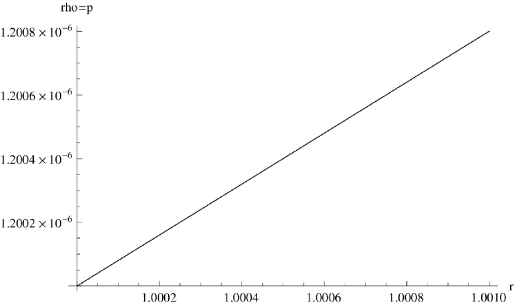
Figure 1: Variations in the profile of density relationship with respect to $r$

3.3 Region III

As discussed earlier, it is seen that in the region III, one needs to take $\rho=P=0$ . In this framework, we consider a vacuum exterior region that can be illustrated through a Schwarzschild solution as follows

$$ds^{2}_{+}=\left(1-\frac{2M}{r}\right)dt^{2}-\left(1-\frac{2M}{r}\right)^{-1}dr^{2}-r^{2}(d\theta^{2}+\sin^{2}\theta d\phi^{2}),$$ (37)

where $M$ is the total gravitating mass of the system.

4 Junction Conditions

This section is devoted to find the some suitable constraints that can be helpful for the smooth joining of exterior and interior metrics. One can get the required condition with the help of Darmois-Israel formalism [59, 60]. In this formalism, the metric coefficients must be continuous at the junction of two regions at $r=D$ but their derivatives may not be necessarily continuous. Further, working on this formalism we can successfully calculate the stress-energy tensor $S^{i}_{j}$. The Lanczos equation [61, 62, 63, 64] could play a significant role in determining the intrinsic surface stress-energy tensor as follows

$$S^{i}_{j}=-\frac{1}{8\pi}(\kappa^{i}_{j}-\delta^{i}_{j}\kappa^{k}_{k}),$$ (38)

where $\kappa^{i}_{j}=K^{+}_{ij}-K^{-}_{ij}$ which indicates that how much extrinsic curvatures are discontinuous over the boundary surface. Here $-$ sign indicates the interior region and the $+$ shows the exterior region. The second fundamental forms linked with both sides of the shell can be stated as

$$K^{{}^{+}_{-}}_{ij}=-n^{{}^{+}_{-}}_{\nu}\left[\frac{\partial^{2}x_{\nu}}{\partial\xi^{i}\partial\xi^{j}}+\Gamma_{\alpha\beta}^{\nu}\frac{\partial x^{\alpha}}{\partial\xi^{i}}\frac{\partial x^{\beta}}{\partial\xi^{j}}\right]|_{\Sigma},$$ (39)

where $\xi^{i}$ represents the intrinsic coordinates on the shell, $n_{\nu}^{{}^{+}_{-}}$ denotes the unit normal to the surface $\Sigma$. The induced spherically symmetric static metric on the hypersurface takes the form

$$ds^{2}=f(r)dt^{2}-\frac{dr^{2}}{f(r)}-r^{2}(d\theta^{2}+\sin^{2}\theta d\phi^{2}),$$ (40)

and for this type of metric $n_{\nu}^{{}^{+}_{-}}$ can be described as

$$n^{{}^{+}_{-}}_{\nu}=^{+}_{-}|g^{\alpha\beta}\frac{\partial f}{\partial x^{\alpha}}\frac{\partial f}{\partial x^{\beta}}|^{\frac{-1}{2}}\frac{\partial f}{\partial x^{\nu}},$$ (41)

with $n^{\mu}n_{\mu}=1$.

Taking into account the Lanczos equation the stress energy tensor $S^{i}_{j}=diag[\sigma,-\nu,-\nu,-\nu]$ can be easily evaluated. Here, the structural variables, energy density and pressure on the surface are denoted with $\sigma$ and $\nu$, respectively. The generic formula for the computation of surface energy density and the surface pressure can be formulated as under

$$\sigma=\frac{-1}{4\pi D}[\sqrt{f}]^{+}_{-},$$ (42)

$$\nu=\frac{-\sigma}{2}+\frac{1}{16\pi}\left[\frac{f^{\prime}}{\sqrt{f}}\right]^{+}_{-},$$ (43)

By working on Eqs.(42) and (43), we come up with

$$\sigma=\frac{-1}{4\pi D}\left[\sqrt{1-\frac{2M}{D}}-\sqrt{1-\frac{U(D)}{DH}}\right],$$ (44)

$$\nu=\frac{1}{8\pi D}\left[\frac{1-\frac{M}{D}}{\sqrt{1-\frac{2M}{D}}}-\frac{1-\frac{3U(D)}{2DH}+\frac{U^{\prime}(D)}{2H}}{\sqrt{1-\frac{U(D)}{DH}}}\right].$$ (45)

where

$$U(D)=\int[\rho_{0}(\chi_{1}-\chi_{3})+D_{0}]\frac{D^{2}}{H}dr.$$

With the help of the definition of surface energy density, the mass of thin shell can be found as under

$$m_{s}=4\pi D^{2}\sigma=D\left[\sqrt{1-\frac{U(D)}{DH}}-\sqrt{1-\frac{2M}{D}}\right],$$ (46)

where

$$M=\frac{U(D)}{2H}+m_{s}\sqrt{1-\frac{U(D)}{HD}}-\frac{m_{s}^{2}}{2D},$$ (47)

describes the total amount of matter distribution within the static irrotational spherically symmetric gravastars.

4.1 Constant $R,~{}T$ and $Q$

In this background, Eqs.(44) and (45) give

$$\sigma=\frac{-1}{4\pi D}\left[\sqrt{1-\frac{2M}{D}}-\sqrt{1-\frac{D^{2}[\rho_{0}(\chi_{1}-\chi_{3})+D_{0}}{3H}}\right],$$ (48)

$$\nu=\frac{1}{8\pi D}\left[\frac{1-\frac{M}{D}}{\sqrt{1-\frac{2M}{D}}}-\frac{1-\frac{2D^{2}[\rho_{0}(\chi_{1}-\chi_{3})+D_{0}]}{3H}}{\sqrt{1-\frac{D^{2}[\rho_{0}(\chi_{1}-\chi_{3})+D_{0}]}{3H}}}\right],$$ (49)

while an equation analogous to Eq.(46) is found to be

$$m_{s}=4\pi D^{2}\sigma=D\left[\sqrt{1-\frac{D^{2}[\rho_{0}(\chi_{1}-\chi_{3})+D_{0}]}{3H}}-\sqrt{1-\frac{2M}{D}}\right],$$ (50)

where

$$M=\frac{D^{3}[\rho_{0}(\chi_{1}-\chi_{3})+D_{0}]}{6H}+m_{s}\sqrt{1-\frac{D^{2}[\rho_{0}(\chi_{1}-\chi_{3})+D_{0}]}{3H}}-\frac{m_{s}^{2}}{2D},$$ (51)

indicates the total amount of fluid configurations inside the static non-rotating self-gravitating spherical gravastar like structures.

As described by Yousaf et al. [27], to match the exterior and interior metrics at the hyper-surface, the following two conditions should be fulfilled for the thin shell at the boundary

$$f_{,RR}[\partial_{y}R|_{-}^{+}=0,\quad f_{,RR}K^{*}_{\lambda\sigma}|_{-}^{+}=0,\quad f_{,QQ}[\partial_{y}Q|_{-}^{+}=0,\quad K|_{-}^{+}=0,$$ (52)

along with

$$R|_{-}^{+}=0,\quad Q|_{-}^{+}=0,$$ (53)

where $K^{*}_{\lambda\sigma}$ and $K$ are the trace-free and trace components of the extrinsic curvature tensor. These equations describe the matching conditions for $f(R,T,Q)$ theory, provided $f_{,RR}\neq 0$ and $f_{,QQ}\neq 0$ are fulfilled. For the continuity of $R$ and $Q$ in an environment of thin shells, the fulfillment of Eqs.(52) and (53) at the boundary is required.

The above mentioned conditions have been evaluated by Yousaf et al. [27]. They considered the interior, exterior and the induced metrics for the cylindrically symmetric regions involving the non-dissipative anisotropic matter. Then, they developed the dynamical equations using the perturbation scheme and the contraction of Bianchi identities.

5 Physical Features Of The Model

This section is devoted to analyze few characteristics in order to model a viable and well-consistent spherically symmetric isotropic gravastar.

5.1 Shell’s Proper Length

The proper length of the shell can be calculated from the outer boundary of interior region $r=D$ to the outer boundary of the shell $r=D+\epsilon$ where $\epsilon\ll 1$ and indicates the small variations. Here, we shall denote length with the letter $l$. Thus, one can define proper length between the two surfaces as follows

$$l=\int_{D}^{D+\epsilon}\sqrt{e^{\lambda}}dr=\int_{D}^{D+\epsilon}\frac{dr}{\sqrt{2\ln[r]+\frac{r^{2}\psi_{1}}{2H}+C}}.$$ (54)

As the integration of the above equation is not possible, therefore, we shall solve this problem through numerical technique. We have plotted a graph in order to see the physical applicability of such results on the structure of gravastars. In Fig.(2), we have seen the abrupt change in the radial profile of gravastars, which is what we expect for the gravastars structures.

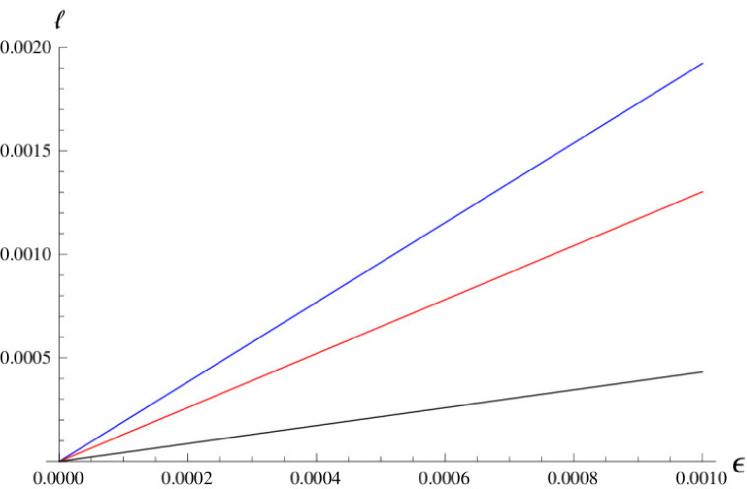
Figure 2: Proper length versus the thickness of the shell

5.2 Energy Content

Energy of the gravastar comes from the inner region having the equation of state $\rho=-P$ . The negative pressure shows here the repulsive nature of the energy which desist to form the singularity in gravastar. However, the energy within the shell comes out to be

$$\varepsilon=\int_{D}^{D+\epsilon}\rho^{(eff)}r^{2}dr=\int_{D}^{D+\epsilon}\frac{Z(2+r^{2}\psi_{1})r}{\psi_{3}}dr.$$ (55)

By considering the thin shell approximation, we have numerically solved the above equation and draw the corresponding graph. The Fig.(3) indicates the direct relationship of the shell with its thickness.

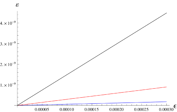
Figure 3: Graph for energy related with thickness of the shell

5.3 Entropy

According to the model of gravastar presented by Mazur and Mottola [28], the entropy $S$ of the shell can be found from the following formula as

$$S=\int_{D}^{D+\epsilon}s(r)r^{2}\sqrt{e^{\lambda}}dr,$$ (56)

where $s(r)$ denotes the entropy density and can be expressed as follows

$$s(r)=\frac{\alpha^{2}k_{B}^{2}T(r)}{4\pi\hbar^{2}}=\alpha\left(\frac{k_{B}}{\hbar}\right)\sqrt{\frac{p^{(eff)}}{2\pi}}.$$ (57)

where $\alpha$ is a dimensionless constant. In the present work, we shall use geometric as well as Planckian units, under which one needs to take $G=c=1$ along with $k_{B}=\hbar=1$. Then the entropy density takes the form

$$s(r)=\alpha\sqrt{\frac{p^{(eff)}}{2\pi}}.$$ (58)

Then Eq.(56) takes the form

$$S=\int_{D}^{D+\epsilon}\frac{\alpha}{\sqrt{2\pi}}\sqrt{\frac{Z(2+r^{2}\psi_{1})}{\psi_{3}r}}r^{2}\frac{1}{\sqrt{2\ln[r]+\frac{r^{2}\psi_{1}}{2H}}+C}dr.$$ (59)

We have plotted a figure (4) in order to study the extend of disorderness for the isotropic spherical gravastars with respect to shell thickness. One can notice from the Fig.(4) that the entropy of the spherical gravastars is turned out to be zero which the corresponding shell thickness is zero. This is one of viable criteria for the single condensate state of celestial object as provided by [mazur2004gravitational].

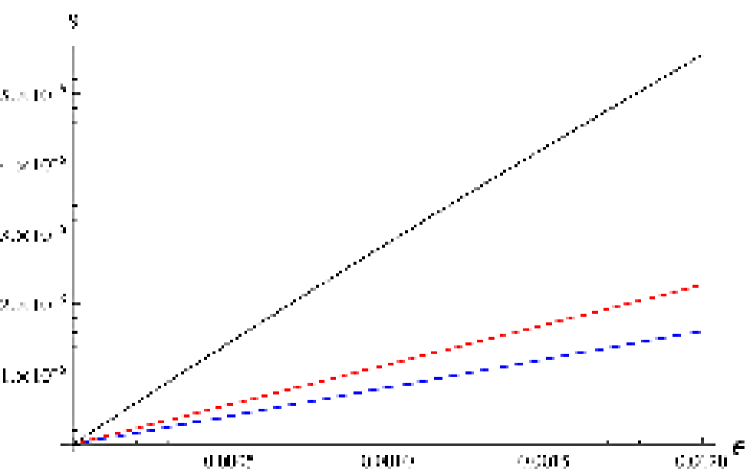
Figure 4: Graph for entropy related with thickness of the shell

5.4 Equation Of State

One can define barotropic EoS at $r=D$ with respect to the effective variables as

$$\nu=\omega(D)\sigma.$$ (60)

This equation relates the state variables which could help us to describe the physical properties of the system. In our system the state variables are surface energy density and surface pressure. With the help of Eqs.(44) and (45), the state parameter can be found as

$$\omega(D)=\frac{1}{2}\left[\frac{\frac{1-\frac{M}{D}}{\sqrt{1-\frac{2M}{D}}}-\frac{1-\frac{3U(D)}{2HD}+\frac{U^{\prime}(D)}{2H}}{\sqrt{1-\frac{U(D)}{HD}}}}{\sqrt{1-\frac{U(D)}{H}-\sqrt{1-\frac{2M}{D}}}}\right].$$ (61)

To obtain real values of $\omega(D)$, the terms appearing in the numerator and denominator of Eq.(61) are to be taken positive. After applying the binomial series on Eq.(61), we have

$$\omega(D)\approx\frac{1}{2}\left[\frac{2H-HD\frac{U^{\prime}(D)}{U(D)}-\frac{U^{\prime}(D)}{2}}{\frac{2MH}{U(D)}-1}\right].$$ (62)

It can be analyzed from Eq.(62), that the constraints $\frac{M}{U(D)}>1$ along with $2>D\frac{U^{\prime}(D)}{U(D)}+\frac{U^{\prime}(D)}{2H}$ and $\frac{M}{U(D)}<1$ with $2<D\frac{U^{\prime}(D)}{U(D)}+\frac{U^{\prime}(D)}{2H}$ will give positive value to $\omega(D)$, while $\omega(D)$ will have a negative value for $\frac{M}{U(D)}>1$ along with $2<D\frac{U^{\prime}(D)}{U(D)}+\frac{U^{\prime}(D)}{2H}$ and $\frac{M}{U(D)}<1$ along with $2>D\frac{U^{\prime}(D)}{U(D)}+\frac{U^{\prime}(D)}{2H}$ relations. In view of present choices of curvature variables, the state parameter can be expressed as

$$\omega(D)=\frac{1}{2}\left[\frac{\frac{1-\frac{M}{D}}{\sqrt{1-\frac{2M}{D}}}-\frac{1-\frac{2D^{2}[\rho_{0}(\chi_{1}-\chi_{3})+D_{0}]}{3H}}{\sqrt{1-\frac{D^{2}[\rho_{0}(\chi_{1}-\chi_{3})+D_{0}]}{3H}}}}{\sqrt{1-\frac{D^{2}[\rho_{0}(\chi_{1}-\chi_{3})+D_{0}]}{3H}-\sqrt{1-\frac{2M}{D}}}}\right],$$ (63)

In order to avoid complex values of $\omega(D)$, we need to take positive values of numerator and denominator of the above expression. After the application of binomial series on the numerator and denominator of Eq.(63), one can find that

$$\omega(D)\approx\frac{1}{2}\left[\frac{3}{\frac{6HM}{D^{3}[\rho_{0}(\chi_{1}-\chi_{3})+D_{0}]}-1}\right],$$ (64)

In Eq.(64), the positive value of $\omega(D)$ can be achieved by taking $\frac{M}{D^{3}}>\frac{\rho_{0}(\chi_{1}-\chi_{3})+D_{0}}{6H}$, while its negative can be observed on taking $\frac{M}{D^{3}}<\frac{\rho_{0}(\chi_{1}-\chi_{3})+D_{0}}{6H}$. The positive (for instance +1) and the negative values of $\omega(D)$ (for example -1) could provide an effective platform to model interior and thin shell of gravastars. Such kind of situations might be useful to understand the mathematical modeling of spherical relativistic isotropic gravastars.

6 Conclusion

This paper is devoted to analyze the role of $f(R,T,Q)$ theory on the formation of relativistic isotropic gravastars. The structures like gravastar, has been considered to be an alternative form of the black hole. To inspect gravastar in this modified theory, we considered suitable static metric (which is spherically symmetric) and then determined its metric coefficients for the three regions separately. Afterwards the physical characteristics edify the substantial results. The outer to boundary surface has been taken to be vacuum. For this purpose, we have considered a Schwarzschild space time and match it by evaluating mathematical constraints presented by Israel and Darmois. With this background, we calculated a set of the collapsing star’s exact and singularity-free models that could help to portrays physically reasonable aspects of gravastars in $f(R,T,Q)$ gravity. These are given as follows:
(1)Description of Pressure and Density: We choose an arbitrary value of radius $r$ and its parameters, by doing that we deduced the effective density and effective pressure displayed persistent deviation even in the presence of $f(R,T,Q)$ theory. In the present paper, we found that at radius $r=1.0010$, the value of density is $\rho=1.2008\times 10^{-6}$. This shows negligible change in the density, while Yousaf [53] found that at $r=1$ the value of density is $\rho=1.32$, which indicates the small but considerable change in the density.
(2)Proper Length: We have studied the behavior of the proper length in account of shell thickness. Under the discussion of the effective matter, Fig.(2) indicates that the length of the shell increases in correspondence to its thickness. This result is also consistent with the results obtained by Yousaf [53] for cylindrical gravastar structures in $f(R,T)$ gravity. In this work, the thickness of the shell is found to be $\epsilon=0.0010$ for the length $\ell=0.0018$, while Yousaf [53] declared $\epsilon$ to be $1.0$ for $0.4$ length $\ell$.
(3)Energy: A graph describing the variation of the energy with respect to the shell thickness in the presence of $f(R,T,Q)$ terms has been drawn and mentioned in Fig(3). The graph confirms the direct proportionality between the energy and thickness of the shell in the presence of effective matter. In this paper, the negligible thickness, i.e., $\epsilon=0.00030km$ gives the small amount of energy i.e., $\varepsilon=4\times 10^{-9}$. while, Yousaf [53] found a large amount of energy within the shell, (i.e., $\varepsilon=250$) at the small thickness of the shell (i.e., $\epsilon=1.4$).
(4)Entropy: We have plotted a graph describing a relation of entropy of the system with the inner shell. Figure (4) indicates that the entropy enhances the thickness of the shell, thus enhancing its role under the influence of effective matter. In the recent paper at thickness $\epsilon=0.0010$, we found the value of the corresponding entropy to be $S=5\times 10^{-6}$. However, Yousaf [53] found the entropy of the shell to be $S=0.5$ for the thickness $\epsilon=1.4$.
(5)Equation of State: We have also computed the ranges of equation of state parameter, under which it is positive or negative. From Eq.(64), we have noticed that the constraint $\frac{M}{D^{3}}>\frac{\rho_{0}(\chi_{1}-\chi_{3})+D_{0}}{6H}$ will give us the positive value of state parameter, while its negative value can be observed on taking $\frac{M}{D^{3}}<\frac{\rho_{0}(\chi_{1}-\chi_{3})+D_{0}}{6H}$.

Acknowledgments

The works of ZY and MZB were supported by National Research Project for Universities (NRPU), Higher Education Commission, Islamabad under the research project No. 8754/Punjab/NRPU/R&D /HEC/2017.

Appendix

The values of $\chi_{i}^{\prime}s$ where $i=1,2,3,...,9,10$ and $D_{j}$ where $j=0,1,2$ appearing in equations (11), (12) and (13) represent the effects of $f(R,T,Q)$ and the dark source, respectively.

$$\chi_{1} =(f_{T}+\frac{Rf_{Q}}{2}+1+f_{T}e^{-\nu}+\frac{\nu^{\prime}\lambda^{\prime}f_{Q}e^{-\nu}}{8}-\frac{3\nu^{\prime\prime}f_{Q}e^{-\lambda}}{4}-\frac{3\nu^{\prime}f_{Q}e^{-\lambda}}{2r}+\frac{f_{Q}^{\prime\prime}e^{-\lambda}}{2}$$

$$-\frac{3\nu^{\prime 2}e^{-\lambda}f_{Q}}{8}-\frac{f_{Q}^{\prime}\lambda^{\prime}e^{-\lambda}}{4}+\frac{e^{-\lambda}f_{Q}^{\prime}}{r}+\frac{\nu^{\prime}\lambda^{\prime}f_{Q}e^{\nu-\lambda}}{4}),$$

$$\chi_{2} =f_{Q}^{\prime}e^{-\lambda}-\frac{f_{Q}\lambda^{\prime}e^{-\lambda}}{4}+\frac{f_{Q}e^{-\lambda}}{r},$$

$$\chi_{3} =\frac{-f_{Q}^{\prime\prime}e^{-\lambda}}{2}+\frac{f_{Q}^{\prime}\lambda^{\prime}e^{-\lambda}}{4}-\frac{\lambda^{\prime}\nu^{\prime}e^{-\nu}f_{Q}}{8}+\frac{\nu^{\prime\prime}e^{-\lambda-\nu}f_{Q}}{4}-\frac{f_{Q}^{\prime}e^{-\lambda}}{r}+\frac{\nu^{\prime}e^{-\nu-\lambda}f_{Q}}{2}$$

$$+\frac{\nu^{\prime 2}e^{-\lambda}f_{Q}}{8},$$

$$\chi_{4} =-f_{Q}^{\prime}e^{-\lambda}+\frac{f_{Q}\lambda^{\prime}e^{-\lambda}}{4}-\frac{f_{Q}e^{-\lambda}}{r},$$

$$D_{0} =\frac{f}{2}-\frac{f_{R}R}{2}+f_{R}^{\prime\prime}e^{-\lambda}-\frac{e^{-\lambda}f_{R}^{\prime}\lambda^{\prime}}{2}+\frac{2e^{-\lambda}f_{R}^{\prime}}{r}.$$

$$\chi_{5} =-f_{T}-\frac{e^{-\lambda}f_{Q}^{\prime}\nu^{\prime}}{4}-\frac{\lambda^{\prime}\nu^{\prime}f_{Q}e^{-\nu}}{8}+\frac{\nu^{\prime\prime}f_{Q}e^{-\lambda}}{4}+\frac{f_{Q}\nu^{\prime}e^{-\lambda}}{2r}+\frac{\nu^{\prime 2}f_{Q}e^{-\lambda}}{8},$$

$$\chi_{6} =f_{T}+\frac{Rf_{Q}}{2}+1+\frac{f_{Q}^{\prime}\nu^{\prime}e^{-\lambda}}{4}+\frac{3\lambda^{\prime}\nu^{\prime}f_{Q}e^{-\lambda}}{8}-\frac{3\nu^{\prime\prime}f_{Q}e^{-\lambda}}{4}+\frac{\nu^{\prime}f_{Q}e^{-\lambda}}{r}$$

$$-\frac{3\nu^{\prime 2}e^{-\lambda}f_{Q}}{8}+\frac{2\lambda^{\prime}f_{Q}e^{-\lambda}}{r},$$

$$\chi_{7} =\frac{\lambda^{\prime}f_{Q}e^{-\lambda}}{4}+\frac{\nu^{\prime}f_{Q}e^{-\lambda}}{4}+\frac{2f_{Q}e^{-\lambda}}{r},$$

$$D_{1} =\frac{-f}{2}+\frac{Rf_{R}}{2}-\frac{\nu^{\prime}f_{R}^{\prime}e^{-\lambda}}{2}-\frac{2f_{R}^{\prime}e^{-\lambda}}{r},$$

$$\chi_{8} =-f_{T}+\frac{f_{Q}^{\prime}\nu^{\prime}e^{-\lambda}}{4}-\frac{\lambda^{\prime}\nu^{\prime}e^{-\nu}f_{Q}}{8r^{2}}+\frac{\nu^{\prime\prime}f_{Q}e^{-\lambda}}{4}+\frac{\nu^{\prime}f_{Q}e^{-\lambda}}{2r}+\frac{\nu^{\prime 2}e^{-\lambda}f_{Q}}{8},$$

$$\chi_{9} =f_{T}+\frac{Rf_{Q}}{2}+1+f_{Q}^{\prime\prime}e^{-\lambda}-\frac{f_{Q}^{\prime}\lambda^{\prime}e^{-\lambda}}{2}+\frac{3f_{Q}^{\prime}\nu^{\prime}e^{-\lambda}}{4}-\frac{f_{Q}^{\prime}\nu^{\prime}e^{-\lambda}}{8}+\frac{\nu^{\prime\prime}e^{-\lambda}f_{Q}}{4}$$

$$-\frac{f_{Q}\nu^{\prime}e^{-\lambda}}{2r}+\frac{\nu^{\prime 2}e^{{}^{-\lambda}f_{Q}}}{8}+\frac{f_{Q}^{\prime}e^{-\lambda}}{r}+\frac{2f_{Q}}{r^{2}}-\frac{2f_{Q}e^{-\lambda}}{r^{2}}+\frac{\lambda^{\prime}f_{Q}e^{-\lambda}}{r},$$

$$\chi_{10} =\frac{3\nu^{\prime}f_{Q}e^{-\lambda}}{4}+\frac{3f_{Q}e^{-\lambda}}{r}+2f_{Q}^{\prime}e^{-\lambda}-\frac{f_{Q}e^{-\lambda}\lambda^{\prime}}{2},$$

$$D_{2} =\frac{-f}{2}+\frac{f_{R}R}{2}-\frac{f_{R}^{\prime}e^{-\lambda}\nu^{\prime}}{2}-f_{R}^{\prime\prime}e^{-\lambda}+\frac{e^{-\lambda}f_{R}^{\prime}\lambda^{\prime}}{2}-\frac{e^{-\lambda}f_{R}^{\prime}}{r}.$$

This is the value of $Z$ which has been appeared in non-conserved (15) shows the effects of modified theory along with dark source effects.

$$Z =\frac{2}{2+Rf_{Q}+2f_{T}}\left[\rho^{\prime}f_{Q}e^{-\lambda}(-\nu^{\prime\prime}-\frac{\nu^{\prime 2}}{2}+\frac{\nu^{\prime}\lambda^{\prime}}{2}-\frac{2\nu^{\prime}}{r})-\frac{f_{Q}Pe^{-\lambda}\nu^{\prime\prime}\lambda^{\prime}}{2}\right.$$

$$-\rho^{\prime}f_{T}-\rho f_{T}^{\prime}-\frac{f_{T}\rho^{\prime}}{2}+\frac{f_{T}P^{\prime}}{2}-\frac{f_{Q}P^{\prime}}{r^{2}}\left(1-e^{-\lambda}-\frac{re^{-\lambda}\nu^{\prime}}{2}\right)-\frac{f_{T}e^{\nu}P^{\prime}}{r^{2}}$$

$$+\frac{f_{Q}^{\prime}\rho e^{-\lambda}}{r^{2}}\left(-1+e^{\lambda}-\nu^{\prime}r\right)+\frac{e^{-\lambda}f_{Q}\rho}{r^{2}}\left(-1+e^{\lambda}-\nu^{\prime}r\right)-\frac{Pf_{Q}e^{-\lambda}\lambda^{\prime}\nu^{\prime 2}}{4}$$

$$+\frac{Pf_{Q}e^{-\lambda}\lambda^{\prime 2}\nu^{\prime}}{4}+\frac{Pf_{Q}e^{-\lambda}\lambda^{\prime 2}}{r}-\frac{f_{Q}e^{-\lambda}\nu^{\prime\prime}P^{\prime}}{4}-\frac{f_{Q}e^{-\lambda}\nu^{\prime 2}P^{\prime}}{8}$$

$$+\frac{f_{Q}e^{-\lambda}\nu^{\prime}\lambda^{\prime}P^{\prime}}{8}+\frac{Pf_{Q}\nu^{\prime\prime}e^{-\lambda}}{r}-\frac{Pf_{Q}\nu^{\prime}\lambda^{\prime}e^{-\lambda}}{r}-\frac{Pf_{Q}e^{-\lambda}\nu^{\prime}}{r^{2}}$$

$$+\left.\frac{2Pf_{Q}}{r^{3}}-\frac{2Pf_{Q}e^{-\lambda}}{r^{3}}+f_{T}^{\prime}P+\frac{f_{Q}^{\prime}P}{2}\left(\frac{2\nu^{\prime}e^{-\lambda}}{r}-\frac{2}{r^{2}}+\frac{2e^{-\lambda}}{r^{2}}\right)\right].$$

References

- [1] D. Pietrobon, A. Balbi, and D. Marinucci Phys. Rev. D, vol. 74, p. 043524, 2006.
- [2] T. Giannantonio et al. Phys. Rev. D, vol. 74, p. 063520, 2006.
- [3] A. G. Riess et al. Astrophys. J., vol. 659, p. 98, 2007.
- [4] S. Nojiri and S. D. Odintsov Phys. Rev. D, vol. 74, no. 8, p. 086005, 2006.
- [5] E. J. Copeland, M. Sami, and S. Tsujikawa Int. J. Mod. Phys. D, vol. 15, p. 1753, 2006.
- [6] K. Bamba, S. Capozziello, S. Nojiri, and S. D. Odintsov Astrophys. Space Sci., vol. 342, p. 155, 2012.
- [7] S. Nojiri and S. D. Odintsov Phys. Rep., vol. 505, p. 59, 2011.
- [8] S. Nojiri, S. D. Odintsov, and V. K. Oikonomou Phys. Rep., vol. 692, p. 1, 2017.
- [9] S. Capozziello and V. Faraoni, Beyond Einstein gravity: A Survey of gravitational theories for cosmology and astrophysics, vol. 170. Springer Science & Business Media, 2010.
- [10] S. Capozziello and M. De Laurentis Phys. Rep., vol. 509, p. 167, 2011.
- [11] A. De Felice and S. Tsujikawa Living Rev. Relativ., vol. 13, p. 3, 2010.
- [12] A. Joyce, B. Jain, J. Khoury, and M. Trodden Phys. Rep., vol. 568, p. 1, 2015.
- [13] Y.-F. Cai, S. Capozziello, M. De Laurentis, and E. N. Saridakis Rep. Prog. Phys., vol. 79, p. 106901, 2016.
- [14] Z. Yousaf, K. Bamba, and M. Z. Bhatti Phys. Rev. D, vol. 93, p. 124048, 2016.
- [15] Z. Yousaf, K. Bamba, and M. Z. Bhatti Phys. Rev. D, vol. 93, p. 064059, 2016.
- [16] K. Bamba and S. D. Odintsov Symmetry, vol. 7, p. 220, 2015.
- [17] M. F. Shamir and A. Malik Comm. Theor. Phys., vol. 71, p. 599, 2019.
- [18] T. Harko, F. S. N. Lobo, S. Nojiri, and S. D. Odintsov Phys. Rev. D, vol. 84, p. 024020, 2011.
- [19] Z. Haghani, T. Harko, F. S. N. Lobo, H. R. Sepangi, and S. Shahidi Phys. Rev. D, vol. 88, p. 044023, 2013.
- [20] I. Ayuso, J. B. Jiménez, and Á. de la Cruz-Dombriz Phys. Rev. D, vol. 91, p. 104003, 2015.
- [21] S. D. Odintsov and D. Sáez-Gómez Phys. Lett B, vol. 725, p. 437, 2013.
- [22] E. H. Baffou, M. J. S. Houndjo, and J. Tosssa Astrophys. Space Sci., vol. 361, p. 376, 2016.
- [23] G. Dvali New J. Phys., vol. 8, p. 326, 2006.
- [24] Z. Yousaf, M. Z. Bhatti, and U. Farwa Class. Quantum Grav., vol. 34, p. 145002, 2017.
- [25] Z. Yousaf, M. Z. Bhatti, and U. Farwa Mon. Not. Roy. Astron. Soc., vol. 464, p. 4509, 2016.
- [26] Z. Yousaf, K. Bamba, M. Z. Bhatti, and U. Farwa Eur. Phys. J. A, vol. 54, p. 122, 2018.
- [27] Z. Yousaf, M. Z. Bhatti, and U. Farwa Eur. Phys. J. C, vol. 77, p. 359, 2017.
- [28] P. O. Mazur and E. Mottola Proc. Natl. Acad. Sci. U.S.A, vol. 101, p. 9545, 2004.
- [29] K. S. Virbhadra, D. Narasimha, and S. M. Chitre Astron. Astrophys., vol. 337, p. 1, 1998.
- [30] K. S. Virbhadra and G. F. R. Ellis Phys. Rev. D, vol. 65, p. 103004, 2002.
- [31] M. Z. Bhatti and Z. Yousaf Int. J. Mod. Phys. D, vol. 26, p. 1750045, 2017.
- [32] Z. Yousaf, M. Z. Bhatti, and M. F. Malik Eur. Phys. J. Plus, vol. 134, p. 470, 2019.
- [33] Z. Yousaf, M. Z. Bhatti, and S. Yaseen Eur. Phys. J. Plus, vol. 134, p. 487, 2019.
- [34] M. Z. Bhatti, Z. Yousaf, and M. Yousaf Phys. Dark Universe, vol. 28, p. 100501, 2020.
- [35] M. Visser and D. L. Wiltshire Class. Quantum Grav., vol. 21, no. 4, p. 1135, 2004.
- [36] C. Cattoen, T. Faber, and M. Visser Class. Quantum Grav., vol. 22, no. 20, p. 4189, 2005.
- [37] C. B. M. H. Chirenti and L. Rezzolla Class. Quantum Grav., vol. 24, p. 4191, 2007.
- [38] N. Bilić, G. B. Tupper, and R. D. Viollier J. Cosmol. Astropart. Phys., vol. 2006, p. 013, 2006.
- [39] D. Horvat, S. Ilijić, and A. Marunović Class. Quantum Grav., vol. 28, p. 195008, 2011.
- [40] N. Sakai, H. Saida, and T. Tamaki Phys. Rev. D, vol. 90, p. 104013, 2014.
- [41] C. B. Chirenti and L. Rezzolla Phys. Rev. D, vol. 78, p. 084011, 2008.
- [42] F. Rahaman, A. A. Usmani, S. Ray, and S. Islam Phys. Lett. B, vol. 717, p. 1, 2012.
- [43] P. Pani, E. Berti, V. Cardoso, Y. Chen, and R. Norte Phys. Rev. D, vol. 80, p. 124047, 2009.
- [44] S. Ghosh, F. Rahaman, B. Guha, and S. Ray Phys. Lett. B, vol. 767, p. 380, 2017.
- [45] A. Das, S. Ghosh, B. Guha, S. Das, F. Rahaman, and S. Ray Phys. Rev. D, vol. 95, p. 124011, 2017.
- [46] M. F. Shamir and M. Ahmad Phys. Rev. D, vol. 97, p. 104031, 2018.
- [47] Z. Yousaf Astrophys. Space Sci., vol. 363, p. 226, 2018.
- [48] Z. Yousaf Eur. Phys. J. Plus, vol. 134, p. 245, 2019.
- [49] Z. Yousaf, K. Bamba, M. Z. Bhatti, and U. Ghafoor Phys. Rev. D, vol. 100, p. 024062, 2019.
- [50] M. Z. Bhatti, Z. Yousaf, and M. Ajmal Int. J. Mod. Phys. D, vol. 28, p. 1950123, 2019.
- [51] M. Z. Bhatti Mod. Phys. Lett. A, vol. 34, p. 2050069, 2020.
- [52] M. Sharif and A. Waseem Astrophys. Space Sci., vol. 364, p. 189, 2019.
- [53] Z. Yousaf Phys. Dark Universe, vol. 28, p. 100509, 2020.
- [54] Y. B. Zeldovich Mon. Not. Roy. Astron. Soc., vol. 160, p. 1P, 1972.
- [55] M. S. Madsen, J. P. Mimoso, J. A. Butcher, and G. F. R. Ellis Phys. Rev. D, vol. 46, p. 1399, 1992.
- [56] P. S. Wesson Vistas Astron., vol. 29, p. 281, 1986.
- [57] T. M. Braje and R. W. Romani Astrophys. J., vol. 580, p. 1043, 2002.
- [58] L. P. Linares, M. Malheiro, and S. Ray Int. J. Mod. Phys. D, vol. 13, p. 1355, 2004.
- [59] W. Israel Nuovo Cimento B, vol. 44, no. 1, 1966.
- [60] G. Darmois Gauthier-Villars, Paris, vol. 25, 1927.
- [61] K. Lanczos Ann. Phys.(Berl.), vol. 379, p. 518, 1924.
- [62] N. Sen Ann. Phys.(Berl.), vol. 378, p. 365, 1924.
- [63] G. Perry and R. B. Mann Gen. Relativ. Gravit., vol. 24, p. 305, 1992.
- [64] P. Musgrave and K. Lake Class. Quantum Grav., vol. 13, p. 1885, 1996.