Stability of Gravastars with Exterior Regular Black Holes

Abstract

This paper examines the stability of thin-shell gravastars in the context of regular spacetimes (Bardeen and Bardeen-de Sitter black holes). We apply cut and paste approach to construct gravastars through the matching of interior non-singular de Sitter geometry with exterior regular black hole. This model contains three regions, i.e., interior, thin-shell and exterior. The interior and exterior regions are connected at thin-shell. We investigate physical viability of the developed model by the energy conditions and explore its stability by using radial perturbation about the equilibrium shell radius. It is found that thin-shell gravastars show large stable regions for the Bardeen-de Sitter black hole as compared to the Bardeen black hole. It is concluded that stable regions exist near the formation of expected event horizon.

Keywords: Gravastars; Israel thin-shell formalism; Stability analysis.
PACS: 04.40.Dg; 04.40.Nr; 04.70.Bw; 97.10.Cv;

1 Introduction

The final outcome of the gravitational collapse of massive objects containing singularity at their center are referred to as black holes (BHs). These compact objects are surrounded by a boundary from which nothing can escape, not even light known as the event horizon. It is a one-way membrane that allows only to move inside the BH and acts as a barrier between interior and exterior geometries. Mazur and Mottola [1] proposed a new image of the collapse by extending the concept of Bose-Einstein condensation to gravitational systems known as gravitational vacuum star (gravastar) [2]. They used cut and paste method to obtain the geometrical structure of thin-shell gravastars. These geometries are interesting because they could address two basic issues, one being the challenge of singularity while another is an information loss paradox related to BH spacetimes. Such a geometrical structure does not contain the central singularity and event horizon.

Gravastar has de Sitter geometry as an interior spacetime while the usual BH as an exterior spacetime like Schwarzschild BH. The interior and exterior regions are partitioned through a thin layer of matter surface known as thin-shell. The following geometrical structure can be characterized into three regions with different equations of state (EoS). Mathematically, these EoS can be defined as

• For interior region ($0\leq r<r_{1}$), $p=-\sigma$.

• For thin-shell ($r_{1}<r<r_{2}$), $p=\sigma$.

• For exterior region ($r_{2}<r$), $p=0=\sigma$.

Here, $p$ is the surface pressure and $\sigma$ is the surface energy density while $r_{1}-r_{2}$ represents thickness of the shell. The presence of matter distribution has great importance to maintain the stable configuration of a thin-shell that produces enough pressure to counterbalance the effect of gravitational force. The characteristics of matter distribution can be determined by using Israel formalism [3]. The cut and paste approach eliminates the singularity and event horizon in the geometrical structure of gravastars [4]. This technique has also been applied to construct thin-shell wormholes from different BHs [5].

Many researchers have studied the new image of gravastar through various approaches. Visser and Wiltshire [6] developed thin-shell gravastars from the joining of interior and exterior spacetimes using cut and paste approach. They also investigated the stable structure through radial perturbation for some specific EoS. Carter [7] studied the stability of thin-shell gravastars by using EoS with different exterior geometries. Bil$\acute{i}$c et al. [8] introduced a new type of gravastars by replacing de Sitter interior geometry with Born-Infled phantom. Horvat et al. [9] extended the concept of gravastars by considering Reissner-Nordström spacetime as an exterior geometry. Usmani et al. [10] also proposed charged gravastars and studied the entropy of the system. Banerjee et al. [11] introduced an alternative of braneworld BHs as braneworld gravastars and also explored their physical characteristics.

G$\acute{a}$sp$\acute{a}$r and R$\acute{a}$cz [12] observed the stability of gravastars through the inelastic collision of their surface layer with a dust shell. Horvat et al. [13] considered the gravastar with continuous pressure and examined stability through the conventional Chandrasekhar approach. Lobo and Garattini [14] found the exact solutions of gravastars in noncommutative geometry and studied their physical characteristics. They explored the dynamical stability of the transition layer for some specific cases and found that stable regions are enhanced near the formation of the expected event horizon. Lobo et al. [15] explored the stability of gravastars related to the matter distribution in the transition layer. Övgün et al. [16] constructed thin-shell gravastars in the background of noncommutative geometry and examined stability regions through radial perturbation about the equilibrium shell radius. Shamir and Ahmad [17] discussed various physical characteristics like, entropy, the EoS parameter, length of the shell, energy-thickness relation of the gravastar shell model in $f(G,T)$ gravity. Yousaf et al. [18] examined the stable regions of gravastar and its characteristics in the background of $f(R,T)$ gravity. Sharif and Waseem [19] explored the charged gravastars with conformal motion in $f(R,T)$ gravity.

A regular BH is an outcome of multiple attempts to establish a feasible interior structure by avoiding the singularity. Bardeen [20] was the pioneer to introduce exact solutions of the field equations that contain event horizon with regular center. Later, some other models of regular BHs were proposed [21]. Moreno and Sarbach [22] investigated the dynamical stability of regular BHs with respect to arbitrary linear fluctuations of the metric and the electromagnetic field. Zhou et al. [23] observed the behavior of the effective potential for the particles and photons in the spacetime of Bardeen BH. Fernando [24] studied the Bardeen BH in de Sitter and anti-de Sitter spacetimes. Recently, Li et al. [25] examined thermodynamical stability of Bardeen BH through heat capacity as well as Gibbs free energy and also discussed thermodynamics of Bardeen-AdS BH.

The cosmological constant ($\Lambda$) is an important parameter to investigate thin-shell stability. Eiroa and Romero [26] examined the stability of thin-shell wormholes constructed from different BHs. They found stable static solutions with Chaplygin gas model for different values of charge as well as $\Lambda$. Lobo and Crawford [27] studied stability of spherical thin-shell wormholes in the presence of $\Lambda$ and found that stable regions are enhanced for large positive value of $\Lambda$. We also analyzed the linearized stability of thin-shell wormholes developed from Bardeen and Bardeen-de Sitter BHs with variable EoS [28]. It is found that thin-shell becomes more stable in the presence of cosmological constant.

Regular BHs motivate to develop thin-shell gravastars by considering regular BHs as an exterior geometry. In this paper, we are interested to examine the stable characteristics of regular thin-shell gravastars through radial perturbation. The paper has the following format. Section 2 develops the general formalism of thin-shell gravastars through cut and paste approach. Section 3 explains the stability procedure of thin-shell through radial perturbation about the equilibrium shell radius. We also observe the corresponding stable regions of thin-shell gravastars. In the last section, we summarize our results.

2 Exterior of Gravastars: Regular Black Holes

The line element of Bardeen-de Sitter BH can be expressed as [24]

$$ds^{2} = -\left(1-\frac{2r^{2}m}{(r^{2}+Q^{2})^{\frac{3}{2}}}-\frac{\Lambda r^{2}}{3}\right)dt^{2}+\left(1-\frac{2r^{2}m}{(r^{2}+Q^{2})^{\frac{3}{2}}}-\frac{\Lambda r^{2}}{3}\right)^{-1}dr^{2}$$

$$+ r^{2}(d\theta^{2}+\sin^{2}\theta d\phi^{2}),$$

where $\Lambda$, $Q$ and $m$ denote the cosmological constant, charge and total mass of the BH. This spacetime can be reduced in different BH geometries such that

• If $\Lambda=0$ and $Q\neq 0$, then it represents the Bardeen BH [20].

• If $\Lambda=0=Q$, it corresponds to the Schwarzschild BH.

The event horizon ($r_{h}$) of a BH geometry is a point at which the metric function vanishes.

2.1 Geometrical Construction of Gravastars

Here, we briefly discuss the mathematical procedure to develop the geometry of gravastars. We consider non-singular de Sitter geometry as an interior metric and regular BHs as an exterior. The corresponding interior (-) and exterior (+) geometries are expressed by the line element

$$ds^{2}_{\pm}=-\Phi_{\pm}(r_{\pm})dt_{\pm}^{2}+\Phi_{\pm}^{-1}(r_{\pm})dr_{\pm}^{2}+r_{\pm}^{2}(d\theta_{\pm}^{2}+\sin^{2}\theta_{\pm}d\phi_{\pm}^{2}),$$ (1)

where

$$\Phi_{-}(r_{-})=\left(1-\frac{r^{2}_{-}}{\alpha^{2}}\right),\quad\Phi_{+}(r_{+})=\left(1-\frac{2r^{2}_{+}m}{(r^{2}_{+}+Q^{2})^{\frac{3}{2}}}-\frac{\Lambda r^{2}_{+}}{3}\right),$$

and $\alpha$ is a nonzero constant. Visser introduced a well-known approach to develop thin-shell gravastars by the junction of both spacetimes that eliminate the event horizon and singularity. For this purpose, we consider a subset ($\Upsilon^{\pm}$) of these manifolds $(\Pi^{\pm})$ through cut and paste technique that does not contain any type of event horizon as well as singularity, i.e., $\Upsilon^{\pm}\subset\Pi^{\pm}$. Here, $\Upsilon^{\pm}=\{x^{\nu}|r_{\pm}\geq y(\tau)>r_{h}\}$, where $x^{\nu}$, $\tau$ and $y(\tau)$ represent coordinates of the manifold, proper time on the shell and shell radius. These subsets $\Upsilon^{\pm}$ are glued at their common timelike hypersurface $\partial\Upsilon$, i.e., $\partial\Upsilon\subset\Upsilon^{\pm}$. The matching between $\Upsilon^{+}$ and $\Upsilon^{-}$ at throat radius provides a connection between interior and exterior spacetimes ($\partial\Upsilon\equiv\Upsilon^{+}\cup\Upsilon^{-}$) that follow the radial flare-out condition. This manifold ($\partial\Upsilon$) represents a thin-shell gravastar which is geodesically complete.

The corresponding line element of the induced metric at $\partial\Upsilon$ is given in the following form

$$ds^{2}=-d\tau^{2}+y(\tau)^{2}d\theta^{2}+y(\tau)^{2}\sin^{2}\theta d\phi^{2},$$

and the components of unit normals at $\Upsilon_{\pm}$ can be expressed as

$$n_{\pm}^{\mu}=\left(\frac{\dot{y}}{\Phi_{\pm}(y)},\sqrt{\Phi_{\pm}(y)+\dot{y}^{2}},0,0\right),$$

where $\dot{y}=dy/d\tau$. The components of extrinsic curvature are defined as

$$K_{ij}^{\pm}=-n_{\mu}^{\pm}\left(\Gamma^{\mu}_{\alpha\beta}\frac{dx^{\alpha}_{\pm}}{d\eta^{i}}\frac{dx^{\beta}_{\pm}}{d\eta^{j}}+\frac{d^{2}x_{\pm}^{\mu}}{d\eta^{i}d\eta^{j}}\right),\quad\alpha,\beta=0,1,2,3,\quad i,j=0,2,3,$$

and hence

$$K_{\tau}^{\tau\pm}=\frac{\Phi^{\prime}_{\pm}(y)+2\ddot{y}}{\sqrt{\Phi_{\pm}(y)+\dot{y}^{2}}},\quad K_{\theta}^{\theta\pm}=\frac{\sqrt{\Phi_{\pm}(y)+\dot{y}^{2}}}{y},\quad K^{\phi\pm}_{\phi}=\sin^{2}\theta K_{\theta}^{\theta\pm},$$ (2)

where $\Phi^{\prime}_{\pm}(y)=\frac{d\Phi_{\pm}(y)}{dy}$.

The presence of matter surface produces extrinsic curvature discontinuity at the hypersurface and its existence can be evaluted by using Israel formalism. Mathematically, such a matter surface can be observed, if $(K_{ij}^{+}-K_{ij}^{-}\neq 0)$. The characteristics of matter surface located at thin-shell are determined by the field equations for the hypersurface referred to as Lanczos equations

$$S^{i}_{j}=-\frac{1}{8\pi}\{[K^{i}_{j}]-\delta^{i}_{j}K\},$$ (3)

where $S^{i}_{j}$ denotes the energy-momentum tensor for $\partial\Upsilon$, $[K^{i}_{j}]=K^{+i}_{j}-K^{-i}_{j}$ and $K=tr[K_{ij}]=[K^{i}_{j}]$. For perfect fluid distribution, the stress-energy tensor yields

$$S^{i}_{j}=\left(\sigma+p\right)u^{i}u_{j}+p\delta^{i}_{j},$$

here $u_{i}$, $\sigma$ and $p$ denote the components of shell’s velocity, surface energy density and pressure of the matter surface. The corresponding $\sigma$ and $p$ of thin-shell gravastars can be evaluated through the Lanczos equations as

$$\sigma = -\frac{[K^{\theta}_{\theta}]}{4\pi}=-\frac{1}{4\pi y}\left\{\sqrt{\dot{y}^{2}+\Phi_{+}(y)}-\sqrt{\dot{y}^{2}+\Phi_{-}(y)}\right\},$$ (4)

$$p = \frac{[K^{\theta}_{\theta}]+[K_{\tau}^{\tau}]}{8\pi}=\frac{1}{8\pi y}\left\{\frac{2\dot{y}^{2}+2y\ddot{y}+2\Phi_{+}(y)+y\Phi^{\prime}_{+}(y)}{\sqrt{\dot{y}^{2}+\Phi_{+}(y)}}\right.$$ (5)

$$- \left.\frac{2\dot{y}^{2}+2y\ddot{y}+2\Phi_{-}(y)+y\Phi^{\prime}_{-}(y)}{\sqrt{\dot{y}^{2}+\Phi_{-}(y)}}\right\},$$

while

$$\sigma+2p = \frac{1}{4\pi}[K_{\tau}^{\tau}]=\frac{1}{4\pi}\left\{\frac{\Phi^{\prime}_{+}(y)+2\ddot{y}}{\sqrt{\Phi_{+}(y)+\dot{y}^{2}}}-\frac{\Phi^{\prime}_{-}(y)+2\ddot{y}}{\sqrt{\Phi_{-}(y)+\dot{y}^{2}}}\right\}.$$ (6)

Here, we assume that shell’s movement along the radial direction vanishes at equilibrium throat radius say $y_{0}$, i.e., $\dot{y}_{0}=0=\ddot{y}_{0}$. Hence, the above equations can be expressed as

$$\sigma_{0} = -\frac{1}{4\pi y_{0}}\left\{\sqrt{\Phi_{+}(y_{0})}-\sqrt{\Phi_{-}(y_{0})}\right\},$$ (7)

$$p_{0} = \frac{1}{8\pi y_{0}}\left\{\frac{2\Phi_{+}(y_{0})+y_{0}\Phi^{\prime}_{+}(y_{0})}{\sqrt{\Phi_{+}(y_{0})}}-\frac{2\Phi_{-}(y_{0})+y_{0}\Phi^{\prime}_{-}(y_{0})}{\sqrt{\Phi_{-}(y_{0})}}\right\},$$ (8)

and

$$\sigma_{0}+2p_{0}=\frac{1}{4\pi}\left\{\frac{\Phi^{\prime}_{+}(y_{0})}{\sqrt{\Phi_{+}(y_{0})}}-\frac{\Phi^{\prime}_{-}(y_{0})}{\sqrt{\Phi_{-}(y_{0})}}\right\},$$ (9)

where $\sigma_{0}$ and $p_{0}$ are the surface energy density and pressure at $y=y_{0}$, respectively.

2.2 Energy Conditions and Balance Equation

To discuss the physical viability of a model, we impose some geometrical constraints, known as energy conditions. There are four well-known energy conditions null ($\sigma_{0}+p_{0}\geq 0$), weak ($\sigma_{0}\geq 0$, $\sigma_{0}+p_{0}\geq 0$), strong ($\sigma_{0}+3p_{0}\geq 0$) and dominant ($\sigma_{0}\pm p_{0}\geq 0$, $\sigma_{0}\geq 0$). These constraints must be satisfied for normal matter distribution. These energy conditions are satisfied for thin-shell gravastars for some specific conditions given as

If $\sqrt{\frac{\Phi_{+}(y_{0})}{\Phi_{-}(y_{0})}}\leq 1$, then $\sigma_{0}\geq 0$.

If $\sqrt{\frac{\Phi_{+}(y_{0})}{\Phi_{-}(y_{0})}}\leq\frac{\Phi_{+}(y_{0})^{\prime}}{\Phi_{-}(y_{0})^{\prime}}$, then $\sigma_{0}+p_{0}\geq 0$.

If $\sqrt{\frac{\Phi_{+}(y_{0})}{\Phi_{-}(y_{0})}}\leq\frac{4\Phi_{+}(y_{0})+y_{0}\Phi_{+}(y_{0})^{\prime}}{4\Phi_{-}(y_{0})+y_{0}\Phi_{-}(y_{0})^{\prime}}$, then $\sigma_{0}-p_{0}\geq 0$.

If $\sqrt{\frac{\Phi_{+}(y_{0})}{\Phi_{-}(y_{0})}}\leq\frac{4\Phi_{+}(y_{0})+3y_{0}\Phi_{+}(y_{0})^{\prime}}{4\Phi_{-}(y_{0})+3y_{0}\Phi_{-}(y_{0})^{\prime}}$, then $\sigma_{0}+3p_{0}\geq 0$.

Now, we consider the equation that describes characteristics of radial pressure in terms of the total energy-momentum tensor ($T_{\alpha\beta}^{\text{total}}$) at the hypersurface as [29]

$$[T_{\alpha\beta}^{\text{total}}n^{\alpha}n^{\beta}]=\frac{1}{2}S^{i}_{j}(K^{i+}_{j}+K^{i-}_{j}),$$

where the square brackets represent the discontinuity across the shell. By considering the values of extrinsic curvature for interior and exterior spacetimes, we obtain the pressure balance equation as

$$\Delta^{-}(y_{0})-\Delta^{+}(y_{0})=\frac{\sigma_{0}}{2}\left(\frac{\Phi_{+}(y_{0})^{\prime}}{\sqrt{\Phi_{+}(y_{0})}}+\frac{\Phi_{-}(y_{0})^{\prime}}{\sqrt{\Phi_{-}(y_{0})}}\right)+\frac{p_{0}}{2y_{0}}(\sqrt{\Phi_{+}(y_{0})}+\sqrt{\Phi_{-}(y_{0})}).$$ (10)

where $-\Delta^{+}(y_{0})=T_{\alpha\beta}^{\text{total}}n^{\alpha}n^{\beta}$ represents the radial tension acting on the shell. This equation gives the difference between radial tension of interior and exterior geometries in terms of $\sigma_{0}$ and $p_{0}$. It is noted that for the exterior vacuum solution $\Delta^{+}(y_{0})=0$. Here, we consider a particular case, $\sigma=0$ for which Eq.(10) reduces to

$$\Delta^{-}(y_{0})=\frac{p_{0}}{2y_{0}}\left(\sqrt{\Phi_{+}(y_{0})}+\sqrt{\Phi_{-}(y_{0})}\right).$$ (11)

This equation directly relates the interior radial tension $\Delta^{-}(y_{0})$ with a surface pressure of the matter surface located at the shell. If $\Delta^{-}(y_{0})>0$, then $p_{0}>0$, that prevents the geometrical structure of gravastars from collapsing. If $\Delta^{-}(y_{0})<0$, then $p_{0}<0$, that hold the expanding behavior of the shell. The corresponding expansion and collapse of thin-shell gravastars are shown in Figure 1. Initially, thin-shell shows expanding behavior ($p_{0}<0$) and then represents the collapse ($p_{0}>0$).

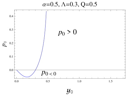
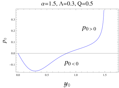
Figure 1: Plots of $p_{0}$ for different values of $\alpha$. These plots show the expanding and collapsing behavior of thin-shell gravastars.

3 Stability Analysis

In this section, we examine the stability of thin-shell gravastars through the radial perturbation about the shell’s radius at the equilibrium position. The dynamical characteristics of thin-shell can be determined through the equation of motion and the conservation equation. These equations have great importance to explore the stable regions of a geometrical structure. Firstly, we derive the equation of motion by rearranging Eq.(4) as

$$\dot{y}^{2}+\Omega(y)=0,$$ (12)

where $\Omega(y)$ is the effective potential that can be expressed as

$$\Omega(y)=\frac{1}{2}\left(\Phi_{-}(y)+\Phi_{+}(y)\right)-\frac{(\Phi_{-}(y)-\Phi_{+}(y))^{2}}{64\pi^{2}y^{2}\sigma^{2}}-4\pi^{2}y^{2}\sigma^{2}.$$ (13)

For Bardeen-de Sitter and Bardeen BHs, the corresponding effective potential become

$$\Omega_{BDS}(y) = 1-4\pi^{2}y^{2}\sigma^{2}-\frac{1}{64\pi^{2}y^{2}\sigma^{2}}\left(\frac{y^{2}}{\alpha^{2}}-\frac{1}{3}y^{2}\left(\Lambda+\frac{6m}{\left(Q^{2}+y^{2}\right)^{3/2}}\right)\right)^{2}$$

$$- \frac{\Lambda y^{2}}{6}-\frac{my^{2}}{\left(Q^{2}+y^{2}\right)^{3/2}}-\frac{y^{2}}{2\alpha^{2}},$$

$$\Omega_{B}(y) = 1-\frac{y^{2}}{2\alpha^{2}}-\frac{ym}{\left(y^{2}+Q^{2}\right)^{3/2}}-\frac{1}{64\pi^{2}\sigma^{2}}\left(\frac{y}{\alpha^{2}}-\frac{2m}{\left(y^{2}+Q^{2}\right)^{3/2}}\right)^{2}$$

$$- 4\pi^{2}y^{2}\sigma^{2},$$

respectively. Also, $\sigma$ and $p$ in terms of potential function can be written as

$$\sigma = -\frac{1}{4\pi y}\left\{\sqrt{\Omega(y)+\Phi_{+}(y)}-\sqrt{\Omega(y)+\Phi_{-}(y)}\right\},$$ (14)

$$p = \frac{2(\Omega+\Phi_{+})+y(\Omega^{\prime}+\Phi^{\prime}_{+})}{8\pi y\sqrt{\Omega(y)+\Phi_{+}(y)}}-\frac{2(\Omega+\Phi_{-})+y(\Omega^{\prime}+\Phi^{\prime}_{-})}{8\pi y\sqrt{\Omega(y)+\Phi_{-}(y)}}.$$ (15)

Secondly, we analyze that $\sigma$ and $p$ follow the conservation equation

$$p\frac{d}{d\tau}(4\pi y^{2})+\frac{d}{d\tau}(4\pi y^{2}\sigma)=0,$$

which leads to

$$\sigma^{\prime}=-\frac{2(\sigma+p(\sigma))}{y}.$$

To observe the stability, we consider radial perturbation through Taylor series up to second-order terms. Therefore, we expand the effective potential about $y=y_{0}$

$$\Omega(y)=\Omega(y_{0})+(y-y_{0})\Omega^{\prime}(y_{0})+\frac{1}{2}(y-y_{0})^{2}\Omega^{\prime\prime}(y_{0})+O[(y-y_{0})^{3}].$$

It is found that $\Omega(y_{0})=0=\Omega^{\prime}(y_{0})$. Consequently, the above equation turns out to be

$$\Omega(y)=\frac{1}{2}(y-y_{0})^{2}\Omega^{\prime\prime}(y_{0}).$$ (16)

As the mass of thin-shell can be expressed as $M(y)=4\pi y^{2}\sigma$, the corresponding second derivative of effective potential at $y=y_{0}$ in terms of $M(y_{0})$ yields

$$\Omega^{\prime\prime}(y_{0}) = \frac{2M(y_{0})M^{\prime}(y_{0})}{y^{3}_{0}}-\frac{y_{0}^{2}(\Phi_{-}(y_{0})-\Phi_{+}(y_{0}))\left(\Phi_{-}(y_{0})^{\prime\prime}-\Phi_{+}(y_{0})^{\prime\prime}\right)}{2M(y_{0})^{2}}$$ (17)

$$+ \frac{2y_{0}^{2}(\Phi_{-}(y_{0})-\Phi_{+}(y_{0}))M^{\prime}(y_{0})\left(\Phi_{-}^{\prime}(y_{0})-\Phi_{+}^{\prime}(y_{0})\right)}{M(y_{0})^{3}}-\frac{M^{\prime}(y_{0})^{2}}{2y_{0}^{2}}$$

$$- \frac{y_{0}^{2}\left(\Phi_{-}^{\prime}(y_{0})-\Phi_{+}^{\prime}(y_{0})\right)^{2}}{2M(y_{0})^{2}}-\frac{3y_{0}^{2}(\Phi_{-}(y_{0})-\Phi_{+}(y_{0}))^{2}M^{\prime}(y_{0})^{2}}{2M(y_{0})^{4}}$$

$$- \frac{2y_{0}(\Phi_{-}(y_{0})-\Phi_{+}(y_{0}))\left(\Phi_{-}^{\prime}(y_{0})-\Phi_{+}^{\prime}(y_{0})\right)}{M(y_{0})^{2}}+\frac{(\Phi_{-}^{\prime\prime}(y_{0})+\Phi_{+}^{\prime\prime}(y_{0}))}{2}$$

$$- \frac{3M(y_{0})^{2}}{2y_{0}^{4}}+\frac{y_{0}^{2}(\Phi_{-}(y_{0})-\Phi_{+}(y_{0}))^{2}M^{\prime\prime}(y_{0})}{2M(y_{0})^{3}}-\frac{M(y_{0})M^{\prime\prime}(y_{0})}{2y_{0}^{2}}$$

$$- \frac{(\Phi_{-}(y_{0})-\Phi_{+}(y_{0}))^{2}}{2M(y_{0})^{2}}+\frac{2y_{0}(\Phi_{-}(y_{0})-\Phi_{+}(y_{0}))^{2}M^{\prime}(y_{0})}{M(y_{0})^{3}},$$

where

$$M^{\prime}(y_{0})=-8\pi y_{0}p_{0},\quad M^{\prime\prime}(y_{0})=-8\pi p_{0}+16\pi\eta_{0}^{2}(\sigma_{0}+p_{0}),$$

here $\eta_{0}^{2}=dp/d\sigma|_{y=y_{0}}$ represents the EoS parameter. The potential function and its second derivative explain the stability of thin-shell gravastars.

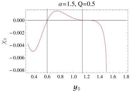
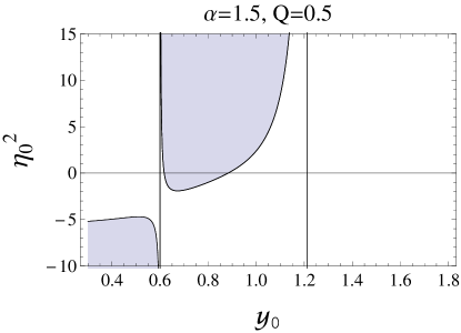
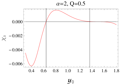
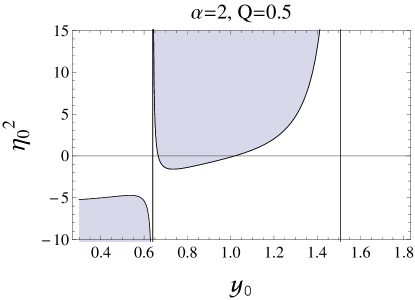
Figure 2: Left and right plots represent the graphical behavior of $\chi_{0}$ and $\eta_{0}^{2}$ for $\Lambda=0$, respectively. In the absence of $\Lambda$, these figures explain the characteristics of thin-shell gravastars for the Bardeen BH. The shaded regions indicate the stable regions.

Figure 3: Left and right plots represent the graphical behavior of $\chi_{0}$ and $\eta_{0}^{2}$ for $\Lambda=0$, respectively.

The stable and unstable structures can be characterized as follows [30]

(i)  If $\Omega^{\prime\prime}(y_{0})>0$, then it shows stable behavior.

(ii)  If $\Omega^{\prime\prime}(y_{0})<0$, it expresses the unstable behavior.

(iii)  If $\Omega^{\prime\prime}(y_{0})=0$, then it is unpredictable.

We are interested in stable configuration of thin-shell gravastars, i.e., $\Omega^{\prime\prime}(y_{0})>0$. Therefore, Eq.(17) can be expressed as

$$\left(-512\pi^{4}y_{0}^{4}(2\eta_{0}^{2}+3)p_{0}\sigma^{5}-256\pi^{4}y_{0}^{4}(4\eta_{0}^{2}+3)\sigma_{0}^{6}-1024\pi^{4}y_{0}^{4}p_{0}^{2}\sigma_{0}^{4}\right.$$

$$+ \left.y_{0}\sigma_{0}\left(y_{0}\sigma_{0}\left(\Phi_{-}(y_{0})^{\prime\prime}\left(16\pi^{2}y_{0}^{2}\sigma_{0}^{2}-\Phi_{-}(y_{0})+\Phi_{+}(y_{0})\right)+\Phi_{+}(y_{0})^{\prime\prime}\left(\Phi_{-}(y_{0})\right.\right.\right.\right.$$

$$+ \left.\left.\left.\left.16\pi^{2}y_{0}^{2}\sigma_{0}^{2}-\Phi_{+}(y_{0})\right)\right)+2\Phi_{-}(y_{0})^{\prime}\left(y_{0}\sigma_{0}\Phi_{+}(y_{0})^{\prime}-2(2p_{0}+\sigma_{0})\left(\Phi_{-}(y_{0})\right.\right.\right.\right.$$

$$- \left.\left.\left.\left.\Phi_{+}(y_{0})\right)\right)-y_{0}\sigma_{0}\left(\Phi_{-}(y_{0})^{\prime}\right)^{2}-y_{0}\sigma_{0}\left(\Phi_{+}(y_{0})^{\prime}\right)^{2}+4(2p_{0}+\sigma_{0})\left(\Phi_{-}(y_{0})\right.\right.\right.$$

$$- \left.\left.\left.\Phi_{+}(y_{0})\right)\Phi_{+}(y_{0})^{\prime}\right)+2(2\eta_{0}^{2}-5)p_{0}\sigma_{0}(\Phi_{-}(y_{0})-\Phi_{+}(y_{0}))^{2}-12p_{0}^{2}\left(\Phi_{-}(y_{0})\right.\right.$$

$$- \left.\left.\Phi_{+}(y_{0})\right)^{2}+(4\eta_{0}^{2}-1)\sigma_{0}^{2}(\Phi_{-}(y_{0})-\Phi_{+}(y_{0}))^{2}\right)(32\pi^{2}y_{0}^{4}\sigma_{0}^{4})^{-1}>0.$$

The stable condition of thin-shell can be written in the following form

$$\Omega^{\prime\prime}(y_{0})<0\quad\Rightarrow\quad\chi(y_{0})\eta_{0}^{2}-\textit{A}(y_{0})<0.$$ (18)

Here, $\chi(y_{0})=\chi_{0}$ is the coefficient of EoS parameter ($\eta_{0}^{2}$) and $\textit{A}(y_{0})=\textit{A}_{0}$ is the remaining term of the above expression in which $\eta_{0}^{2}$ does not involve. We discuss the geometrical behavior of thin-shell gravastars through the stability regions. The stable regions can be characterized as follows

(i)  If $\chi_{0}<0$, then $\eta_{0}^{2}<\textit{A}_{0}/\chi_{0}$.

(ii)  If $\chi_{0}>0$, then $\eta_{0}^{2}>\textit{A}_{0}/\chi_{0}$,

where

$$A_{0} = -256\pi^{4}y_{0}^{4}\sigma_{0}^{4}\left(4p_{0}^{2}+6p_{0}\sigma_{0}+3\sigma_{0}^{2}\right)+y_{0}\sigma_{0}\left(y_{0}\sigma_{0}\left(\Phi_{-}(y_{0})^{\prime\prime}\left(16\pi^{2}y_{0}^{2}\sigma_{0}^{2}\right.\right.\right.$$

$$- \left.\left.\left.\Phi_{-}(y_{0})+\Phi_{+}(y_{0})\right)+\Phi_{+}(y_{0})^{\prime\prime}\left(16\pi^{2}y_{0}^{2}\sigma_{0}^{2}+\Phi_{-}(y_{0})-\Phi_{+}(y_{0})\right)\right)\right.$$

$$+ \left.2\Phi_{-}(y_{0})^{\prime}\left(y_{0}\sigma_{0}\Phi_{+}(y_{0})^{\prime}-2(\Phi_{-}(y_{0})-\Phi_{+}(y_{0}))(2p_{0}+\sigma_{0})\right)\right.$$

$$- \left.y_{0}\sigma_{0}\left(\Phi_{-}(y_{0})^{\prime}\right)^{2}-y_{0}\sigma_{0}\left(\Phi_{+}(y_{0})^{\prime}\right)^{2}+4\Phi_{+}(y_{0})^{\prime}(2p_{0}+\sigma_{0})\left(\Phi_{-}(y_{0})\right.\right.$$

$$- \left.\left.\Phi_{+}(y_{0})\right)\right)-\Phi_{-}(y_{0})^{2}\left(12p_{0}^{2}+10p_{0}\sigma_{0}+\sigma_{0}^{2}\right)+2\Phi_{-}(y_{0})\left(12p_{0}^{2}+\sigma_{0}^{2}\right.$$

$$+ \left.10p_{0}\sigma_{0}\right)\Phi_{+}(y_{0})-\Phi_{+}(y_{0})^{2}\left(12p_{0}^{2}+10p_{0}\sigma_{0}+\sigma_{0}^{2}\right),$$

$$\chi_{0} = 4\sigma_{0}(p_{0}+\sigma_{0})\left((\Phi_{-}(y_{0})-\Phi_{+}(y_{0}))^{2}-256\pi^{4}y_{0})^{4}\sigma_{0}^{4}\right).$$

We explain the stable regions of thin-shell gravastars through the graphical behavior of $\chi_{0}$ and $\eta_{0}^{2}$ for $m=0.5$. We study the effect of $\alpha$, charge and cosmological constant on the geometrical structure of thin-shell gravastars. According to stable condition, if $\chi_{0}>0$ then the stable region is the area above the plots of $A_{0}/\chi_{0}$ and vice-versa. Figure 2 explains that for the left plot $\chi_{0}\leq 0$ if $y_{0}\in[0.2,0.6]$ and $\chi_{0}\geq 0$ if $y_{0}\in[0.6,1.7]$. Thus the stable regions represent the area less than $A_{0}/\chi_{0}$ if $y_{0}\in[0.2,0.6]$ and greater than $A_{0}/\chi_{0}$ if $y_{0}\in[0.6,1.7]$. The point $y_{0}=0.6$ denotes the event horizon at which $A_{0}/\chi_{0}$ becomes infinite. It is found that near the expected event horizon, stability regions must exist. Similarly, we observe the stability regions and corresponding event horizons for different values of $\alpha$, $Q$ and $\Lambda$. Figure 3 shows stable regions are enhanced by increasing $\alpha$ for some specific values of $Q=0.5=m$ while Figure 4 represents the influence of charge on the stability of thin-shell gravastars. It is observed that stable regions are decreased by increasing charge of the exterior geometry. Figure 5 indicates that stable regions are greatly affected by the cosmological constant which shows that stable regions are enhanced with the cosmological constant.

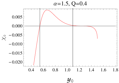
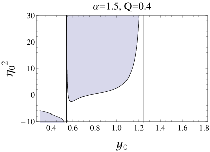
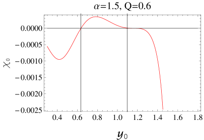
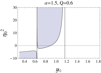
Figure 4: Left and right plots represent the graphical behavior of $\chi_{0}$ and $\eta_{0}^{2}$ for $\Lambda=0$, respectively.

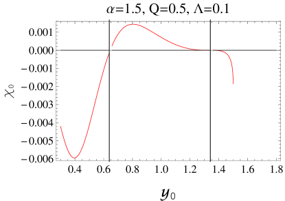
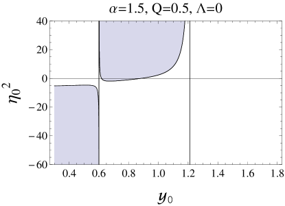
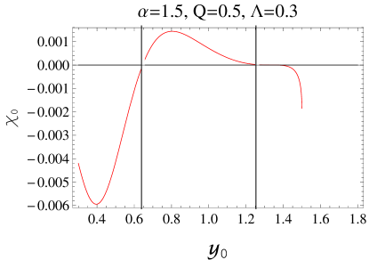
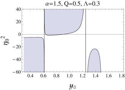
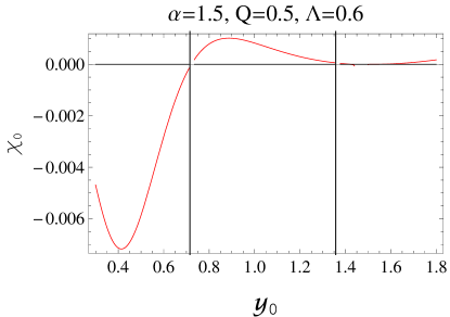
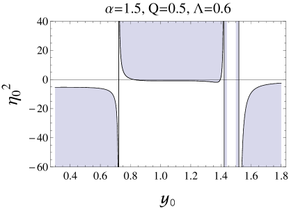
Figure 5: Left and right plots represent the graphical behavior of $\chi_{0}$ and $\eta_{0}^{2}$, respectively. These plots illustrate the effect of $\Lambda$ on the stable behavior of thin-shell gravastars for the Bardeen-de Sitter spacetime.

4 Final Remarks

In this paper, we have studied the stability of a specific class of thin-shell gravastars in the background of regular BHs. For this purpose, we have considered cut and paste approach to develop the geometrical structure of thin-shell gravastars by the matching of interior non-singular de Sitter spacetime with exterior regular BH. The characteristics of matter surface located at thin-shell are determined by using Israel formalism and the Lanczos equations. For the viability of the developed structure, we have examined the energy conditions and found some constraints over the metric functions of both spacetimes. It is observed that thin-shell represents expanding and collapsing behavior (Figure 1).

We have also studied the stable configurations of thin-shell gravastars for the Bardeen and Bardeen-de Sitter geometry as exterior line elements. We have analyzed the stable characteristics of thin-shell gravastars through the radial perturbation about the equilibrium shell radius. The stable regions of thin-shell gravastars are observed through graphs. Figures 2 and 3 indicate that stability of thin-shell gravastars is increased by increasing $\alpha$. For Bardeen BH, it is found that stable regions are decreased by increasing charge of the exterior geometry (Figure 4). For Bardeen-de Sitter BH, stable regions are enhanced with cosmological constant (Figure 5). We would like to mention here that regular BHs as exterior line element of gravastars show more stable behavior. It is concluded that thin-shell gravastars are more stable for the Bardeen-de Sitter BH rather than Bardeen BH.

References

• [1] Mazur, P. and Mottola, E.: arXiv: gr-qc/0109035; Proc. Nat. Acad. Sci. 101(2004)9545.
• [2] Mielke, E.W. and Schunck, F.E.: Nucl. Phys. B 564(2000)185.
• [3] Israel, W.: Nuovo Cimento B 44(1966)1.
• [4] Visser, M., Kar, S. and Dadhich, N.: Phys. Rev. Lett. 90(2003)201102.
• [5] Varela, V.: Phys. Rev. D 92(2015)044002; Sharif, M. and Azam, M.: Eur. Phys. J. C 73(2013)2407; Sharif, M. and Javed, F.: Int. J. Mod. Phys. D 28(2019)1950046; Ann. Phys. 407(2019)198; Chin. J. Phys. 61(2019)262; Mod. Phys. Lett. A 34(2019)1950350; Int. J. Mod. Phys. A doi.org/10.1142/S0217751X20400151.
• [6] Visser, M. and Wiltshire, D.L.: Class. Quantum Grav. 21(2004)1135.
• [7] Carter, B.M.N.: Class. Quantum Grav. 22(2005)4551.
• [8] Bilic, N., Tupper G.B. and Viollier, R.D.: J. Cosmol. Astropart. Phys. 0602(2006)013.
• [9] Horvat, D., Sasa Ilijic, S. and Marunovic, A.: Class. Quantum Grav. 26(2009)025003.
• [10] Usmani et al.: Phys. Lett. B 701(2011)388.
• [11] Banerjee, A., Rahaman, F., Islam, S. and Govender, M.: Eur. Phys. J. C 76(2016)34.
• [12] G$\acute{a}$sp$\acute{a}$r, M.E. and R$\acute{a}$cz, I.: Class. Quantum Grav. 27(2010)185004.
• [13] Horvat, D., Ilijic, S. and Marunovic, A.: Class. Quantum Grav. 28(2011)195008.
• [14] Lobo, F.S.N. and Garattini, R.: J. High Energy Phys. 1312(2013)065.
• [15] Lobo et al.: arXiv:1512.07659.
• [16] Γ–vgΓΌn, A., Banerjee, A. and Jusufi, K.: Eur. Phys. J. C 77(2017)566.
• [17] Shamir, M.F. and Ahmad, M.: Phys. Rev. D 97(2018)104031.
• [18] Yousaf et al.: Phys. Rev. D 100(2019)024062.
• [19] Sharif, M. and Waseem, A.: Astrophys. Space Sci. 364(2019)189.
• [20] Bardeen, J.M.: Proceedings of GR5 (Tiflis, USSR, 1968)174.
• [21] Ay$\acute{o}$n-Beato, E. and Garc$\acute{i}$a, A.: Phys. Rev. Lett. 80(1998)5056; Bronnikov, K.A.: Phys. Rev. Lett. 85(2000)4641; Phys. Rev. D 63(2001)044005; Hayward, S.A.: Phys. Rev. Lett. 96(2006)031103.
• [22] Moreno,C. and Sarbach, O.: Phys. Rev. D 67(2003)024028.
• [23] Zhou, S., Chen, J. and Wang, Y.: Int. J. Mod. Phys. D 21(2012)1250077.
• [24] Fernando, S.: Int. J. Mod. Phys. D 26(2017)1750071.
• [25] Li et al.: Mod. Phys.Lett. A 34(2019)1950336.
• [26] Eiroa, E.F. and Romero, G.E.: Gen. Relativ. Gravit. 36(2004)651.
• [27] Lobo, F.S.N. and Crawford, P.: Class. Quantum Grav. 21(2004)391.
• [28] Sharif, M. and Javed, F.: Gen. Relativ. Gravit. 48(2016)158; Astrophys. Space Sci. 364(2019)179.
• [29] Musgrave, P. and Lake, K.: Class. Quantum Grav. 13(1996)1885.
• [30] Rahaman, F., Banerjee, A. and Radinschi, I.: Int. J. Theor. Phys. 52(2013)2943.