Koopman Operator Methods for Global Phase Space Exploration of Equivariant Dynamical Systems

Abstract

In this paper, we develop the Koopman operator theory for dynamical systems with symmetry. In particular, we investigate how the Koopman operator and eigenfunctions behave under the action of the symmetry group of the underlying dynamical system. Further, exploring the underlying symmetry, we propose an algorithm to construct a global Koopman operator from local Koopman operators. In particular, we show, by exploiting the symmetry, data from all the invariant sets are not required for constructing the global Koopman operator; that is, local knowledge of the system is enough to infer the global dynamics.

1 Introduction

Dynamical systems theory is one of the most important branches of mathematics in the sense that it has applications in almost all fields of science and engineering. Any system which changes with time is a dynamical system and hence, they are ubiquitous in nature. As such, both theoretical and numerical analysis of dynamical systems is important. An important class of dynamical systems are the ones which have a symmetry in the sense that there exists some transformations on the state space which carries one solution of the dynamical system to another solution of the dynamical system Field (1970); Field (1980); Golubitsky et al. (2012) and the symmetries manifest themselves in asymptotic dynamics, bifurcation, attractor structures etc. Chossat and Golubitsky (1988); Sparrow (2012); Mesbahi et al. (2019); Salova et al. (2019). Moreover, symmetries play an important role in synchronization, pattern formation, quantum systems, etc. Mathematically, symmetry is specified by the action of some group on the state space and hence, for studying symmetric dynamical systems, elements of group theory and representation theory are used.

Traditionally, theoretical analysis of dynamical systems is performed by studying the evolution of trajectories in the phase space. However, more recently a different technique is being increasingly used to study dynamical systems, where instead of studying the trajectories in the phase space, the focus is, using transfer operators like Perron-Frobenius operator (P-F) and Koopman operator, on studying the evolution of measures or functions defined on the phase space Lasota and Mackey (1994); Vaidya and Mehta (2008); Mezić and Banaszuk (2004); Mezić (2005); Mehta and Vaidya (2005); Budisic et al. (2012).

The main advantage of this approach is the fact that the evolution of measures or functions is linear in the infinite-dimensional space. Moreover, the evolution of functions, which is governed by the Koopman operator, is tailor-made for data-driven analysis of dynamical systems. This is especially useful for analysis of higher dimensional systems like power networks, building systems, biological networks, etc. However, one drawback of using transfer operators is that these are typically infinite-dimensional operators. Hence, for data-driven analysis researchers have developed many different methods for computing the finite-dimensional approximations of these transfer operators and using the developed framework for analysis and control of dynamical systems Dellnitz and Junge (1999); Mezic and Banaszuk (2000); Froyland (2001); Junge and Osinga (2004); Mezić and Banaszuk (2004); Dellnitz et al. (2005); Mezić (2005); Mehta and Vaidya (2005); Vaidya and Mehta (2008); Raghunathan and Vaidya (2014); Susuki and Mezic (2011); Budisic et al. (2012); Mauroy and Mezic (2013); Surana and Banaszuk (2016); Yeung et al. (2018); Yeung et al. (2017); Sinha et al. (2019b); Johnson and Yeung (2018); Sinha et al. (2018b); Sinha et al. (2018a); Sinha et al. (2019a).

In this paper, we use the Koopman operator framework to study dynamical systems with symmetry. In particular, we analyze some basic properties of symmetric dynamical systems and their symmetry group and investigate how these properties are reflected on the infinite-dimensional Koopman operator for the corresponding symmetric dynamical systems. In particular, we analyze how the symmetry of the underlying system affects the evolution of functions in the function space under the action of the Koopman operator. Moreover, as mentioned before, Koopman operator techniques facilitate the data-driven analysis of dynamical systems. To this end, in this paper, we use the construction technique proposed in Nandanoori et al. (2019) to provide a method for constructing the global Koopman operator (defined on the entire phase space) from local Koopman operators (defined on locally invariant sets). In particular, we show that using the symmetry of the underlying system, one does not need to train the local Koopman operators on all the different invariant spaces and hence, one does not need the data from all the invariant subspaces for constructing the global operator.

2 Preliminaries

In this section, we discuss the preliminaries of equivariant systems and transfer operators.

2.1 Equivariant Dynamical Systems

Consider a dynamical system

$$\dot{x}=f(x)$$ (1)

where $x\in M\subseteq\mathbb{R}^{n}$ and $f:M\to M$ is assumed to be at least $\mathcal{C}^{1}$. A symmetry of the dynamical system (1) is a transformation that maps solutions of the system to other solutions of the system. A dynamical system with such a transformation is known as an equivariant dynamical system and is defined as follows:

Definition 1 (Equivariant Dynamical System)

Consider the dynamical system (1) and let $G$ be a group acting on $M$. The system is called $G$-equivariant if

$$f(g\cdot x)=g\cdot f(x),\;\text{for}\;g\in G,x\in M,$$

that is, the following diagram commutes for every $g\in G$.

The definition for an equivariant discrete-time dynamical system $x_{t+1}=T(x_{t})$ is defined analogously. In particular, a discrete time dynamical system $x_{t+1}=T(x_{t})$ is $G$-equivariant if

$$T(g\cdot x)=g\cdot T(x)\;\text{for}\;g\in G.$$ (2)

Note that, for a solution $x(t)$ of Eq. (1), $g\cdot x(t)$ is also a solution, with the same being true for discrete-time dynamical system.

Example 1

Consider the Lorenz system given by

$$\begin{aligned} \dot{x}=&\sigma(y-x)\\ \dot{y}=&x(\rho-z)-y\\ \dot{z}=&xy-\beta z\end{aligned}$$ (3)

where $\sigma$, $\rho$ and $\beta$ are constants. The system equations remain invariant under the transformation $(x,y,z)\mapsto(-x,-y,z)$ and hence the Lorenz system is invariant under the transformation matrix

$$\gamma=\begin{pmatrix}-1&0&0\\ 0&-1&0\\ 0&0&1\end{pmatrix}.$$ (4)

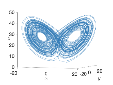
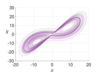
Figure 1: (a) Phase portrait of the Lorenz system (b) Projection of phase portrait on the $x-y$ plane.

Note that $\gamma^{2}=I$, where $I$ is the identity matrix and this transformation corresponds to a $\pi$ rotation about the $z$-axis. Hence, the Lorenz system is invariant under the group $G=\mathbb{Z}_{2}$ action, where the action of the non-identity element is given by rotation of $\pi$ about the $z$-axis and $\gamma$ in Eq. (4) is the $3$-dimensional representation of the non-identity element of $G$.

In this paper, we assume $G$ to be a finite subgroup of $O(n)$ and $M\subset\mathbb{R}^{n}$ to be a compact $G$-invariant set. In general, a symmetry group can be any subgroup of the group of isometries of the Euclidean space $\mathbb{E}^{n}$, but in this work, we consider finite subgroups of the group of point symmetries of $\mathbb{E}^{n}$. Further, we consider discrete-time systems of the form

$$x_{t+1}=T(x_{t}).$$ (5)

Remark 1

We consider discrete-time systems because Koopman operators are tailor-made for data-driven analysis of dynamical systems and data (from a simulation or from an experiment) is always in the form of a discrete time-series.

Also, given an abstract group $G$, let $\Gamma$ be the $n$-dimensional representation of the group $G$ in $\mathbb{R}^{n}$, such that $g\mapsto\gamma_{g}$, where $g\in G$ and $\gamma_{g}\in\Gamma$. Note that, $\gamma_{g}$ has the matrix representation $\gamma_{g}\in\mathbb{R}^{n\times n}$ and the action of the abstract group $G$ on the state space $\mathbb{R}^{n}$ is specified by the action of the representation group $\Gamma$ acting on $\mathbb{R}^{n}$, where the action is by matrix multiplication.

Definition 2 (Isotropy Set)

Let $x_{0}(t)$ be a solution (trajectory) of $G$-equivariant dynamical system (5) from the initial condition $x_{0}$. Then the isotropy set is defined as

$$\Sigma_{x_{0}(t)}=\{g\in G|g\cdot x_{0}(t)=x_{0}(t)\}.$$

With this we have the following.

Lemma 1

The isotropy set corresponding to a solution $x_{0}(t)$ is a subgroup of the symmetry group $G$.

Let $g_{1},g_{2}\in\Sigma_{x_{0}(t)}$. Then, we have

$$g_{1}\cdot[g_{2}\cdot x_{0}(t)]=g_{1}\cdot x_{0}(t)=x_{0}(t).$$

Therefore, $g_{1}\cdot g_{2}\in\Sigma_{x_{0}(t)}$ and hence $\Sigma_{x_{0}(t)}$ is closed. Associativity follows directly. Similarly, the identity element belongs to $\Sigma_{x_{0}(t)}$. Now, suppose $g\in\Sigma_{x_{0}(t)}$ and let $g_{e}$ denote the identity element in $G$. Then, we have

$$x_{0}(t)=g_{e}\cdot x_{0}(t)=g^{-1}g\cdot x_{0}(t)=g^{-1}\cdot x_{0}(t).$$

Therefore, for every $g\in\Sigma_{x_{0}(t)}$, $g^{-1}\in\Sigma_{x_{0}(t)}$. Hence $\Sigma_{x_{0}(t)}$ is a subgroup of $G$.

Proposition 1

Let $\Sigma_{x_{0}(t)}$ and $\Sigma_{gx_{0}(t)}$ be the isotropy groups of $x_{0}(t)$ and $gx_{0}(t)$ respectively. Then we have

$$\Sigma_{gx_{0}(t)}=g\Sigma_{x_{0}(t)}g^{-1}.$$

Let $\theta\in\Sigma_{x_{0}(t)}$, that is, $\theta$ fixes $x_{0}(t)$. Then for $g\in G$,

$$(g\cdot\theta\cdot g^{-1})\cdot(g\cdot x_{0}(t))=g\cdot\theta\cdot x_{0}(t)=g\cdot x_{0}(t).$$

Therefore, $g\cdot\theta\cdot g^{-1}\in\Sigma_{gx_{0}(t)}$. Similarly, for $\sigma\in\Sigma_{gx_{0}(t)}$, $g^{-1}\cdot\sigma\cdot g\in\Sigma_{x_{0}(t)}$. Hence, we obtain

$$\Sigma_{gx_{0}(t)}=g\Sigma_{x_{0}(t)}g^{-1}.$$

2.2 Transfer Operators

In this subsection, we briefly discuss the transfer operators, namely the Perron-Frobenius (P-F) and Koopman operator. Consider a discrete-time dynamical system

$$x_{t+1}=T(x_{t})$$ (6)

where $T:M\subset\mathbb{R}^{N}\to M$ is assumed to be at least $\mathcal{C}^{1}$. Associated with the dynamical system (6) is the Borel-$\sigma$ algebra ${\mathcal{B}}(M)$ on $M$ and the vector space ${\mathcal{M}}(X)$ of bounded complex valued measures on $M$. With this, two linear operators, namely, Perron-Frobenius (P-F) and Koopman operator, can be defined as follows Lasota and Mackey (1994):

Definition 3

The P-F operator $\mathbb{P}:{\mathcal{M}}(X)\to{\mathcal{M}}(X)$ is given by

$$[\mathbb{P}\mu](A)=\int_{{M}}\delta_{T(x)}(A)d\mu(x)=\mu(T^{-1}(A))$$

$\delta_{T(x)}(A)$ is stochastic transition function which measure the probability that point $x$ will reach the set $A$ in one time step under the system mapping $T$.

Definition 4

Invariant measures are the fixed points of the P-F operator $\mathbb{P}$ that are also probability measures. Let $\bar{\mu}$ be the invariant measure then, $\bar{\mu}$ satisfies

$$\mathbb{P}\bar{\mu}=\bar{\mu}.$$

If the state space $X$ is compact, it is known that the P-F operator admits at least one invariant measure.

Definition 5

Given any $h\in\mathcal{F}$, $\mathbb{U}:{\mathcal{F}}\to{\mathcal{F}}$ is defined by

$$[\mathbb{U}h](x)=h(T(x))$$

where $\mathcal{F}$ is the space of functions (observables) invariant under the action of the Koopman operator.

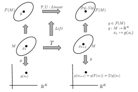
Figure 2: Schematic of the P-F and Koopman operators.

Both the Perron-Frobenius and the Koopman operators are linear operators, even if the underlying system is nonlinear. But while analysis is made tractable by linearity, the trade-off is that these operators are typically infinite-dimensional. In particular, the P-F operator and Koopman operator often will lift a dynamical system from a finite-dimensional space to generate an infinite-dimensional linear system in infinite dimensions (see Fig. 2).

If the P-F operator is defined to act on the space of densities, that is, $L_{1}(M)$ and Koopman operator on space of $L_{\infty}(M)$ functions, then it can be shown that the P-F and Koopman operators are dual to each other.

$$\left<\mathbb{U}f,g\right>=\int_{M}[\mathbb{U}f](x)g(x)dx$$

$$= \int_{M}f(y)g(T^{-1}(y))\left|\frac{dT^{-1}}{dy}\right|dy=\left<f,\mathbb{P}g\right>.$$

where $f\in L_{\infty}(M)$ and $g\in L_{1}(M)$ and the P-F operator on the space of densities $L_{1}(M)$ is defined as follows

$$[\mathbb{P}g](x)=g(T^{-1}(x))\left|\frac{dT^{-1}(x)}{dx}\right|.$$

In the next section, we establish the properties of the Koopman operator for an equivariant dynamical system.

3 Koopman Operator and Equivariant Dynamical Systems

We begin this section with the analysis of group action on a Koopman operator.

3.1 Group Action and Koopman Operator

Suppose

$$x_{t+1}=T(x_{t})$$ (7)

be a dynamical system defined on the state space $M\subset\mathbb{R}^{n}$, which is symmetric with respect to a group $G$ and let $\mathbb{U}$ be the associated Koopman operator. The Koopman operator, $\mathbb{U}$ is a linear operator on the space of functions $({\mathcal{F}}(M))$ on $M$. We define a map

$$\varphi: G\times{\mathcal{F}}(M)\to{\mathcal{F}}(M)$$ (8)

$$(g\star f)(x)\mapsto f(g^{-1}\cdot x).$$

Lemma 2

The map $\varphi$, defined in Eq. (8) defines a group action on the space ${\mathcal{F}}(M)$

Firstly, let $e$ be the identity element of $G$. Then

$$(e\star f)(x)=f(e^{-1}\cdot x)=f(x).$$

Secondly, let $g_{1},g_{2}\in G$ and let $g_{1}\odot g_{2}=g_{3}\in G$, where $\odot$ denotes the group operation. Then

$$[g_{1}\star(g_{2}\star f)](x)=[g_{1}\star f](g_{2}^{-1}\cdot x)=f(g_{1}^{-1}\cdot(g_{2}^{-1}\cdot x))$$

$$\qquad=f((g_{2}^{-1}\odot g_{1}^{-1})\cdot x)=f((g_{1}\odot g_{2})^{-1}\cdot x)$$

$$\qquad=[(g_{1}\odot g_{1})\star f](x).$$

Hence the map $\phi$, defined in (8) defines a group action on ${\mathcal{F}}(M)$.

Now a Koopman operator is a linear operator on ${\mathcal{F}}(M)$. Hence, from the action of the symmetry group $G$ on ${\mathcal{F}}(M)$, we have the following theorem.

Theorem 1

Let $\mathbb{U}$ be the Koopman operator associated with a $G$-equivariant system $x_{t+1}=T(x_{t})$. Then

$$[g\star(\mathbb{U}f)](x)=[\mathbb{U}(g\star f)](x).$$ (9)

for all $g\in G$ and $f\in{\mathcal{F}}(M)$.

For the dynamical system $x_{t+1}=T(x_{t})$ and any function $f\in{\mathcal{F}}(M)$, the Koopman operator $\mathbb{U}$ is defined as $[\mathbb{U}f](x)=f(T(x))$. Hence, for $g\in G$ we have,

$$g\star({\mathbb{U}}f)(x) =g\star f(T(x))=f(g^{-1}\cdot T(x))$$

$$=f(T(g^{-1}\cdot x))={\mathbb{U}}f(g^{-1}\cdot x)=[\mathbb{U}(g\star f)](x),$$

where the third equality follows from the definition of $G$-equivariant systems (refer Eq. (2)). The above theorem essentially says that the Koopman operator commutes with the elements of the symmetry group $G$.

Associated with a Koopman operator is its eigenspectrum, that is, the eigenvalues $\lambda$, and their corresponding eigenfunctions $\phi_{\lambda}(x)$, such that

$$[{\mathbb{U}}\phi_{\lambda}](x)=\lambda\phi_{\lambda}(x).$$

The eigenspectrum (especially eigenfunctions corresponding to dominant eigenvalues) of a Koopman operator dictates the evolution of the functions $f\in{\mathcal{F}}(M)$, under the map $T$ (refer Eq. 7) and hence the different algorithms like Dynamic Mode Decomposition (DMD) Schmid (2010) and Extended Dynamic Mode Decomposition (EDMD) Williams et al. (2015) are geared towards obtaining finite-dimensional approximations of the eigenspectrum of the Koopman operator.

Definition 6

Let ${\mathbb{U}}$ be a Koopman operator and let $\phi_{\lambda}^{i}(x)$ be eigenfunctions of ${\mathbb{U}}$ corresponding to the eigenvalue $\lambda$, that is, ${\mathbb{U}}\phi_{\lambda}^{i}(x)=\lambda\phi_{\lambda}^{i}(x)$. Then the eigenspace ${\mathcal{E}}_{\lambda}$ is defined as

$${\mathcal{E}}_{\lambda}=\textnormal{span}\{\phi_{\lambda}^{i}(x)\}.$$

The following result establishes that the eigenspace is left invariant under group action.

Proposition 2

Let (7) be a $G$-equivariant discrete-time dynamical system and ${\mathbb{U}}$ be the associated Koopman operator. If $\lambda$ is an eigenvalue of the Koopman operator ${\mathbb{U}}$ and ${\mathcal{E}}_{\lambda}$ is the corresponding eigenspace, then the eigenspace remains invariant under the action of the symmetry group $G$.

Let $\phi(x)$ be an eigenfunction of the Koopman operator ${\mathbb{U}}$ with eigenvalue $\lambda$. Then for $g\in G$, we have

$${\mathbb{U}}(g\star\phi(x))=g\star{\mathbb{U}}\phi(x)=g\star\lambda\phi(x)=\lambda(g\star\phi(x))$$ (10)

Hence, if $\phi(x)\in{\mathcal{E}}_{\lambda}$, then $(g\star\phi(x))\in{\mathcal{E}}_{\lambda}$. Hence the eigenspace is left invariant under the $G$-action.

Note that a Koopman operator is a linear operator which gives the evolution of functions which are defined on the state space. Let $x\in M$ and $g\cdot x\in M$ for a $G$-equivariant system (5) and let $f\in L_{2}(M)$. Let $\hat{f}=g\star f$. Then the following proposition relates the representation (analogous to a matrix representation of a linear transformation) of the Koopman operator when the functions $f$ and $\hat{f}$ are evaluated at $x$ and $g\cdot x$ respectively.

Proposition 3

Let (7) be a $G$-equivariant dynamical system and its associated Koopman operator be ${\mathbb{U}}:{\mathcal{F}}(M)\to{\mathcal{F}}(M)$. Suppose $f\in{\mathcal{F}}(M)$ and let ${\mathbb{U}}_{f}$ be the representation of ${\mathbb{U}}$ with respect to $f$. For $g\in G$, let $\hat{f}=g\star f$ and ${\mathbb{U}}_{\hat{f}}$ be the representation of ${\mathbb{U}}$ with respect to $\hat{f}$. Then for $x\in M$, we have

$${\mathbb{U}}_{\hat{f}}\hat{f}(g\cdot x)={\mathbb{U}}_{f}f(x)$$ (11)

We have

$${\mathbb{U}}_{\hat{f}}\hat{f}(g\cdot x)= \hat{f}(T(g\cdot x))=\hat{f}(g\cdot T(x))=g^{-1}\star\hat{f}(T(x))$$

$$= f(T(x))={\mathbb{U}}_{f}f(x).$$

3.2 Group Action and Invariant Spaces

Definition 7

For a dynamical system $x_{t+1}=T(x_{t})$, defined on $M\subseteq\mathbb{R}^{n}$, a subset ${\mathcal{M}}\subset M$ is an invariant set if for every trajectory $x_{0}(t)$,

$$x_{0}(t)\in{\mathcal{M}}\implies x_{0}(\tau)\in{\mathcal{M}},\forall\tau\geq t.$$ (12)

Note that an orbit from an initial condition $x_{0}$ is an invariant set.

For a measure preserving transformation $T$, all the eigenvalues of the associated Koopman operator ${{\mathbb{U}}}$ lie on the unit circle Budisic et al. (2012). Moreover, when $T$ is an ergodic transformation, then all eigenvalues of ${{\mathbb{U}}}$ are simple Petersen (1989); Budisic et al. (2012). However, if $T$ is not ergodic, then the state space can be partitioned into subsets ${\mathcal{M}}_{i}$ (minimal invariant subspaces) such that the restriction $T|_{{\mathcal{M}}_{i}}:{\mathcal{M}}_{i}\to{\mathcal{M}}_{i}$ is ergodic. A partition of the state space into invariant sets is called an ergodic partition or stationary partition. Hence, for any transformation $T$, defined on $M\subseteq\mathbb{R}^{n}$, the state space $M$ can be expressed as

$$M=\cup_{i=1}^{m}{\mathcal{M}}_{i}\textnormal{ (modulo measure zero sets)},$$ (13)

where each ${\mathcal{M}}_{i}$ is an invariant set and ${\mathcal{M}}_{i}$ and ${\mathcal{M}}_{j}$ are disjoint for $i\neq j$. Hence, all ergodic partitions are disjoint and they support mutually singular functions from $L_{2}(M)$ Budisic et al. (2012). Therefore, the number of linearly independent eigenfunctions of ${{\mathbb{U}}}$ corresponding to an eigenvalue $\lambda$ is bounded above by the number of ergodic sets in the state space Budisic et al. (2012). The dynamics of the system dictates the number of ergodic partitions (invariant sets) in the state space. The following results summarize the above discussion.

Lemma 3

Let $\lambda$ be an eigenvalue of the Koopman operator ${\mathcal{K}}$. Suppose if the algebraic multiplicity of the eigenvalue $\lambda$, is equal to the geometric multiplicity, then the corresponding eigenfunctions are linearly independent.

The proof follows from standard results on matrices Horn and Johnson (2012).

Definition 8

Let ${\mathcal{M}}_{i}$ be an invariant set of the $G$-equivariant dynamical system (7). Then for $g\in G$, define the set $g\cdot{\mathcal{M}}_{i}$ as

$$g\cdot{\mathcal{M}}_{i}:=\{\tilde{x}\in M|\tilde{x}=g\cdot x\textnormal{ for }x\in{\mathcal{M}}_{i}\}$$

Proposition 4

If ${\mathcal{M}}_{i}$ is an invariant set for a $G$-equivariant dynamical system $x_{t+1}=T(x_{t})$, then $g\cdot{\mathcal{M}}_{i}$ is also an invariant set for $g\in G$.

For $g\in G$, from the definition of $g\cdot{\mathcal{M}}_{i}$, for any $\tilde{x}\in g\cdot{\mathcal{M}}_{i}$, there exists some $x\in{\mathcal{M}}_{i}$ such that $\tilde{x}=g\cdot x$. Let $\tilde{x}_{0}\in g\cdot{\mathcal{M}}_{i}$ such that $\tilde{x}_{0}=g\cdot x_{0}$ for some $x_{0}\in{\mathcal{M}}_{i}$. Since ${\mathcal{M}}_{i}$ is an invariant set, the trajectory $x_{0}(t)\in{\mathcal{M}}_{i}$. Now,

$$\tilde{x}_{0}(t)= \cup_{t}\{\tilde{x}\in M|\tilde{x}=T^{t}(\tilde{x}_{0}),t\geq 0\}$$

$$= \cup_{t}\{\tilde{x}\in M|\tilde{x}=T^{t}(g\cdot x_{0}),t\geq 0\}$$

$$= \cup_{t}\{\tilde{x}\in M|\tilde{x}=g\cdot T^{t}(x_{0}),t\geq 0\}$$

Now, since ${\mathcal{M}}_{i}$ is an invariant set, $T^{t}(x_{0})\in{\mathcal{M}}_{i}$ and hence, $\tilde{x}_{0}(t)\in g\cdot{\mathcal{M}}_{i}$ and therefore $g\cdot{\mathcal{M}}_{i}$ is invariant.

Corollary 1

For any invariant set ${\mathcal{M}}_{i}$, $G\cdot{\mathcal{M}}_{i}$ is invariant, where

$$G\cdot{\mathcal{M}}_{i}=\{\tilde{x}\in M|\tilde{x}=g\cdot x,\textnormal{ for }x\in{\mathcal{M}}_{i}\textnormal{ and }g\in G\}.$$

4 Global Phase Space Reconstruction from Data

In this section, we develop the data-driven tools for analysis of equivariant dynamical systems.

4.1 Finite Dimensional Approximation of Koopman Operator

Let

$$X_{p}=[x_{1},x_{2},\ldots,x_{M}],\quad X_{f}=[y_{1},y_{2},\ldots,y_{M}]$$ (14)

be snapshots of data obtained from simulating a dynamical system $x\mapsto T(x)$, or from an experiment, where $x_{i}\in M$ and $y_{i}\in M$, $M\subset\mathbb{R}^{n}$. The two pairs of data sets are assumed to be two consecutive snapshots i.e., $y_{i}=T(x_{i})$. Let $\mathcal{D}=\{\psi_{1},\psi_{2},\ldots,\psi_{K}\}$ be the set of observables, where $\psi_{i}:M\to\mathbb{R}$ and $\psi_{i}\in L_{2}(M)$. Let ${\mathcal{G}}_{\mathcal{D}}$ denote the span of ${\mathcal{D}}$. Let $\mathbf{\Psi}:X\to\mathbb{R}^{K}$ be a vector valued function, such that

$$\mathbf{\Psi}(\boldsymbol{x}):=\begin{bmatrix}\psi_{1}(x)&\psi_{2}(x)&\cdots&\psi_{K}(x)\end{bmatrix}^{\top}.$$

Here $\mathbf{\Psi}$ is the mapping from physical space to feature space. Any function $\phi,\hat{\phi}\in\mathcal{G}_{\mathcal{D}}$ can be written as

$$\phi=\sum_{k=1}^{K}a_{k}\psi_{k}=\boldsymbol{\Psi^{T}a},\quad\hat{\phi}=\sum_{k=1}^{K}\hat{a}_{k}\psi_{k}=\boldsymbol{\Psi^{T}\hat{a}}$$ (15)

for some set of coefficients $\boldsymbol{a},\boldsymbol{\hat{a}}\in\mathbb{R}^{K}$. Let $\hat{\phi}(x)=[\mathbb{U}\phi](x)+r,$ where $r$ is a residual that appears because $\mathcal{G}_{\mathcal{D}}$ is not necessarily invariant to the action of the Koopman operator. The finite dimensional approximate Koopman operator $\bf K$ minimizes this residual $r$ and the matrix $\bf K$ is obtained as a solution of the following least square problem:

$$\min\limits_{\bf K}\parallel{\bf K}{Y_{p}}-{Y_{f}}\parallel_{F}$$ (16)

where

$${Y_{p}}={\bf\Psi}(X_{p})= [{\bf\Psi}(x_{1}),{\bf\Psi}(x_{2}),\cdots,{\bf\Psi}(x_{M})]$$ (17)

$${Y_{f}}={\bf\Psi}(X_{f})= [{\bf\Psi}(y_{1}),{\bf\Psi}(y_{2}),\cdots,{\bf\Psi}(y_{M})],$$ (18)

with ${\bf K}\in\mathbb{R}^{K\times K}$. The optimization problem (16) can be solved explicitly to obtain following solution for the matrix $\bf K$

$${\bf K}={Y_{f}}{Y_{p}}^{\dagger}$$ (19)

where ${Y_{p}}^{\dagger}$ is the pseudo-inverse of matrix $Y_{p}$. DMD is a special case of EDMD algorithm with ${\bf\Psi}(x)=x$.

4.2 Global Koopman Operator from Local Koopman Operators

As mentioned earlier, any phase space $M$ can be decomposed into disjoint invariant sets ${\mathcal{M}}_{i}$. Let

$${\bf\Psi}_{i}=\{\psi_{1}^{i},\psi_{2}^{i},\cdots,\psi_{K_{i}}^{i}\}$$ (20)

be the dictionary functions (observables) on each ${\mathcal{M}}_{i}$ and let ${\bf K}_{i}$ be the corresponding Koopman operator on ${\mathcal{M}}_{i}$. Note that, in general, on each ${\mathcal{M}}_{i}$, the dictionary functions are different and hence, the finite-dimensional matrix representation of each of the local Koopman operators ${\bf K}_{i}$ is different. This is because given any linear transformation ${\mathcal{O}}:V\to W$, where $V$ and $W$ are vector spaces, the matrix representation of $\mathcal{O}$ depends on the choice of the basis vectors of $V$ and $W$. For the self-containment of the paper, in this subsection, we briefly review the results of Nandanoori et al. (2019) where we had proposed a systematic method to construct the global Koopman operator ${\bf K}$, which describes the evolution of the system on the entire phase space $M$, from the local Koopman operators ${\bf K}_{i}$.

Let ${\bf\Psi}_{i}$ be the dictionary functions on each invariant set ${\mathcal{M}}_{i}$, $i=1,2,\cdots,m$ and let ${\bf K}_{i}$ be the corresponding Koopman operator which describes the evolution of the system in each ${\mathcal{M}}_{i}$. We define the set of dictionary functions on the entire state space $M$ as

$${\bf\Psi}=\bigsqcup_{i=1}^{m}{\bf\Psi}_{i},$$

where $\bigsqcup$ is the disjoint union. Then if ${\bf K}$ is the global Koopman operator on the entire state space $M$ with dictionary function $\bf\Psi$, then ${\bf K}$ can be expressed as

$${\bf K}=\textnormal{diag}({\bf K}_{1},{\bf K}_{2},\cdots,{\bf K}_{m}).$$ (21)

4.3 Global Koopman Operator for Equivariant Systems

Consider the $G$-equivariant system (7), defined on the state space $M\in\mathbb{R}^{n}$ with disjoint invariant sets ${\mathcal{M}}_{i}$, as in Eq. (13).

From proposition 4 we have that $g\cdot{\mathcal{M}}_{i}$ is also invariant for all $g\in G$. Hence, $g\cdot{\mathcal{M}}_{i}\subset{\mathcal{M}}_{j}$ for some $j\in\{1,2,\cdots,m\}$.

Assumption 1

We assume there exists some $g\in G$, such that $g\cdot{\mathcal{M}}_{i}\subset{\mathcal{M}}_{j}$ and $i\neq j$.

Let ${\bf\Psi}_{i}$ be the dictionary functions defined on ${\mathcal{M}}_{i}$ and let ${\bf K}_{i}$ be the local Koopman operator on ${\mathcal{M}}_{i}$. Let

$$X=[x_{1},x_{2},\cdots,x_{M+1}]$$

be points in ${\mathcal{M}}_{i}$, such that $x_{k+1}=T(x_{k})$ and thus

$$[{\bf K}_{i}{\bf\Psi}_{i}](x_{k})={\bf\Psi}_{i}(x_{k+1}).$$ (22)

Now, ${\bf K}_{j}$ governs the evolution of dictionary functions on ${\mathcal{M}}_{j}$ and the goal is to compute ${\bf K}_{j}$. Since in computing ${\bf K}_{i}$, ${\bf\Psi}_{i}(x_{k})$ are already computed, we would like to use this information for computation of ${\bf K}_{j}$. This can be done in two different ways.

Case I. We use the same dictionary function ${\bf\Psi}_{i}$ on ${\mathcal{M}}_{j}$, that is

$${\bf\Psi}_{j}={\bf\Psi}_{i}.$$

Theorem 2

Let ${\mathcal{M}}_{i}$ be an invariant set of the $G$-equivariant system (7) and let ${\bf K}_{i}\in\mathbb{R}^{K_{i}\times K_{i}}$ be the local Koopman operator on ${\mathcal{M}}_{i}$ with dictionary function ${\bf\Psi}_{i}(x)$, $x\in{\mathcal{M}}_{i}$. Let, for $g\in G$, $g\cdot{\mathcal{M}}_{i}\subset{\mathcal{M}}_{j}$. Let ${\bf K}_{j}$ be the local Koopman operator on ${\mathcal{M}}_{j}$ with dictionary functions ${\bf\Psi}_{j}={\bf\Psi}_{i}$. Then

$${\bf K}_{i}=\gamma{\bf K}_{j}\gamma^{-1},$$

where $g\mapsto\gamma\in\Gamma$ and $\Gamma$ is the $K_{i}$ dimensional matrix representation of $G$ in $\mathbb{R}^{K_{i}}$.

Since ${\bf\Psi}_{j}={\bf\Psi}_{i}$, ${\bf K}_{j}\in\mathbb{R}^{K_{i}\times K_{i}}$. Now consider $x_{k}\in{\mathcal{M}}_{i}$ and $g\cdot x_{k}\in{\mathcal{M}}_{j}$. Then we have,

$${\bf K}_{j}{\bf\Psi}_{i}(g\cdot x_{k})= {\bf\Psi}_{i}(g\cdot x_{k+1})=\gamma^{-1}{\bf\Psi}_{i}(x_{k+1})$$

$$= \gamma^{-1}{\bf K}_{i}{\bf\Psi}_{i}(x_{k}).$$ (23)

Consider again,

$${\bf K}_{j}{\bf\Psi}_{i}(g\cdot x_{k})={\bf K}_{j}\gamma^{-1}{\bf\Psi}_{i}(x_{k}).$$ (24)

Hence, from Eqs. (23) and (24), we have

$${\bf K}_{i}{\bf\Psi}_{i}(x_{k})=\gamma{\bf K}_{j}\gamma^{-1}{\bf\Psi}_{i}(x_{k}).$$ (25)

Since Eq. (25) is true for all $x_{k}\in{\mathcal{M}}_{i}$, we obtain

$${\bf K}_{i}=\gamma{\bf K}_{j}\gamma^{-1}.$$

Corollary 2

Let $x_{0}(t)$ be a trajectory of a $G$-equivariant system $x_{t+1}=T(x_{t})$ and let $g\cdot x_{0}(t)$ be the image of $x_{0}(t)$ under the action of $g\in G$. Let ${\bf\Psi}\in L_{2}(M)$ be a set of dictionary functions of cardinality $K$. Let ${\bf K}_{x_{0}}$ and ${\bf K}_{g\cdot x_{0}}$ be the finite-dimensional representation of Koopman operator which governs the evolution of ${\bf\Psi}$ on $x_{0}(t)$ and $g\cdot x_{0}(t)$ respectively. Then

$${\bf K}_{x_{0}}=\gamma{\bf K}_{g\cdot x_{0}}\gamma^{-1},$$ (26)

where $g\mapsto\gamma\in\Gamma$ and $\Gamma$ is the $K$ dimensional matrix representation of $G$ in $\mathbb{R}^{K}$. Similar to the proof in theorem 2. Note that the local Koopman operators obtained using the DMD algorithm satisfy theorem 2.

Case II. We define the dictionary function on $g\cdot{\mathcal{M}}_{i}$ and hence on ${\mathcal{M}}_{j}$, $j\neq i$ as

$${\bf\Psi}_{j}=g\star{\bf\Psi}_{i}.$$

In this case, from proposition 3, we have

$${\bf K}_{i}={\bf K}_{j}.$$

Hence, starting with an invariant set ${\mathcal{M}}_{i}$, with a local Koopman operator ${\bf K}_{i}$, if $g_{j}\cdot{\mathcal{M}}_{i}\subset{\mathcal{M}}_{j}$ for $j\in\{1,2,\cdots,m\}$, $j\neq i$, we can obtain all the local Koopman operators ${\bf K}_{j}$, $j=1,2,\cdots,m$. Hence, using the procedure of Nandanoori et al. (2019), we can obtain the global Koopman operator, defined on the entire state space $M$ for the $G$-equivariant system (7).

5 Simulation Results

In this section, by applying the symmetry in the system, we identify the global Koopman operator starting from an invariant subspace. We begin with the discussion on systems with reflective symmetry. In all the examples, we use the same dictionary functions on two different invariant spaces (or two different trajectories), which are related by the symmetry group (as in theorem 2).

5.1 Reflection Symmetry: Bistable Toggle Switch

Consider the bistable toggle switch system, first introduced in Gardner et al. (2000). The governing equations of motion are:

$$\dot{x}_{1}= \frac{\alpha_{1}}{1+x_{2}^{\beta}}-\kappa_{1}x_{1}$$ (27)

$$\dot{x}_{2}= \frac{\alpha_{2}}{1+x_{1}^{\theta}}-\kappa_{2}x_{2}$$

where the states $x_{1}\in\mathbb{R}$ and $x_{2}\in\mathbb{R}$ indicate the concentration of the repressor $1$ and $2$; the effective rate of synthesis of repressor $1$ and $2$ are denoted by $\alpha_{1}$ and $\alpha_{2}$; the self decay rates of concentration of repressor $1$ and $2$ are given by $\kappa_{1}>0$ and $\kappa_{2}>0$; the cooperativity of repression of promoter $2$ and $1$ are respectively denoted by $\beta$ and $\theta$.

This system exhibits bistability, that is, this system has two stable equilibrium points and an unstable equilibrium point. The system has two invariant sets and the line $x_{1}=x_{2}$ is the separatrix that separates the two invariant sets. The phase portrait of this system is shown in Fig. 3.

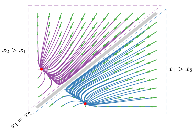
Figure 3: The plane $x_{1}=x_{2}$ acts as a mirror and the phase portrait in the region $x_{2}>x_{1}$ is a mirror reflection of the phase portrait in the region $x_{1}>x_{2}$.

With the given values of the parameters, the system equations are symmetric under the transformation

$$(x_{1},x_{2})^{\top}\xmapsto{\gamma}(x_{2},x_{1})^{\top}.$$ (28)

Hence the symmetry group of the bistable toggle switch is $\mathbb{Z}_{2}$, where the action of the non-identity element of $\mathbb{Z}_{2}$ is given by Eq. (28). In the phase space, this corresponds to a reflection about the $x_{1}=x_{2}$ line and the $2$-dimensional representation of the non-identity element of the symmetry group is

$$\gamma=\begin{pmatrix}0&\;1\\ 1&\;0\end{pmatrix}.$$ (29)

The goal is to construct the global Koopman operator using only the time-series data from any one of the invariant sets. This is achieved in three steps described below:

1. Corresponding to the time-series data from any one of the invariant set, identify the dynamics applying data-driven operator theoretic methods discussed in section 4.1.

2. Identify the dynamics of the other invariant set by noticing that the bistable toggle switch system has reflective symmetry and applying the results from section 4.3.

3. Once the Koopman operators for each invariant set are identified, the global Koopman operator is computed by using the results of the section 4.2.

To demonstrate the proposed framework, we collected time-series data from only the invariant given by the region $x_{1}>x_{2}$. The local Koopman operator, obtained using the DMD algorithm, is given by

$${\bf K}_{right}= \begin{pmatrix}0.6039&0.0313\\ -0.4784&1.0375\end{pmatrix}.$$

Hence, from theorem 2, the Koopman operator corresponding to the region $x_{2}>x_{1}$ can be identified as

$${\bf K}_{left}= \gamma^{-1}{\bf K}_{right}\gamma=\begin{pmatrix}1.0375&-0.4784\\ 0.0313&0.6039\end{pmatrix},$$

where $\gamma$ is given by Eq. (29). Hence the global Koopman operator is

$${\bf K}_{global}=\begin{pmatrix}{\bf K}_{left}&0\\ 0&{\bf K}_{right}\end{pmatrix}.$$

The phase portrait corresponding to the two regions is shown in Fig. 3. Moreover, as a verification, we computed the Koopman operator using data from the region $x_{2}>x_{1}$ and it was equal to

$${\bf K}_{x_{2}>x_{1}}=\begin{pmatrix}1.0375&-0.4784\\ 0.0313&0.6039\end{pmatrix}={\bf K}_{left}.$$

5.2 Rotational Symmetry: Lorenz System

Consider the Lorenz system as shown in Eq. (3) The Lorenz system is symmetric under $\mathbb{Z}_{2}$ action given by

$$(x,y,z)^{\top}\xmapsto{\gamma}(-x,-y,z)^{\top},$$ (30)

which corresponds to a rotation of $180^{\circ}$ about the $z$-axis and matrix representation of $\gamma$ is

$$\gamma=\begin{pmatrix}-1&0&0\\ 0&-1&0\\ 0&0&1\end{pmatrix}.$$ (31)

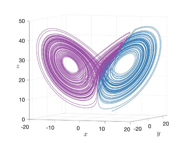
Figure 4: Phase portrait of the Lorenz system.

The phase portrait of the Lorenz system with $\rho=28$, $\sigma=10$ and $\beta=8/3$, is shown in Fig. 4. The colours blue and magenta correspond to the symmetric components of the strange attractor. The Koopman operator computed, using DMD algorithm, from the blue region of the attractor is

$${\bf K}_{blue}=\begin{pmatrix}0.076&0.709&0.042\\ -0.667&1.064&0.124\\ -0.422&0.926&0.836\end{pmatrix}.$$

Hence, from corollary 2, the Koopman on the symmetric counterpart of the blue region will be

$${\bf K}_{magenta}=\gamma^{-1}{\bf K}_{blue}\gamma\\ =\begin{pmatrix}0.076&0.709&-0.042\\ -0.667&1.064&-0.124\\ 0.422&-0.926&0.836\end{pmatrix}$$

which is the same Koopman operator obtained with DMD algorithm with data points on the magenta region of the attractor.

5.3 Reflection and Rotational Symmetry: A Hamiltonian System

Consider a Hamiltonian system with a Hamiltonian

$$H(q,p)=\frac{1}{4}p^{4}-\frac{9}{2}p^{2}-\frac{1}{4}q^{4}+\frac{9}{2}q^{2}.$$

Hence the equations of motion are

$$\dot{q}=\frac{\partial H}{\partial p}=p^{3}-9p;\quad\dot{p}=-\frac{\partial H}{\partial q}=q^{3}-9q.$$ (32)

This system has $4$ invariant sets and the corresponding phase portrait of the system is shown in Fig. 5 and the system is symmetric under the actions given by

$$\begin{pmatrix}q\\ p\end{pmatrix}\xmapsto{\gamma_{1}}\begin{pmatrix}p\\ q\end{pmatrix},\begin{pmatrix}q\\ p\end{pmatrix}\xmapsto{\gamma_{2}}\begin{pmatrix}-q\\ -p\end{pmatrix},\begin{pmatrix}q\\ p\end{pmatrix}\xmapsto{\gamma_{3}}\begin{pmatrix}-p\\ -q\end{pmatrix}.$$ (33)

From the action of $\gamma_{i}$’s, we have

$$\gamma_{1}^{2}=\gamma_{2}^{2}=\gamma_{3}^{3}=I_{2},\textnormal{ and }\gamma_{1}\gamma_{2}=\gamma_{3}.$$

Hence the symmetry group of the system is the Klein 4-group $\mathbb{Z}_{2}\times\mathbb{Z}_{2}$, which has the presentation

$$\Gamma=\langle\gamma_{1},\gamma_{2}|\gamma_{1}^{2}=\gamma_{2}^{2}=(\gamma_{1}\gamma_{2})^{2}=I_{2}\rangle.$$

and the matrix representation of the group elements are

$$\gamma_{1}=\begin{pmatrix}0&1\\ 1&0\end{pmatrix};\gamma_{2}=\begin{pmatrix}-1&0\\ 0&-1\end{pmatrix};\gamma_{3}=\begin{pmatrix}0&-1\\ -1&0\end{pmatrix}.$$

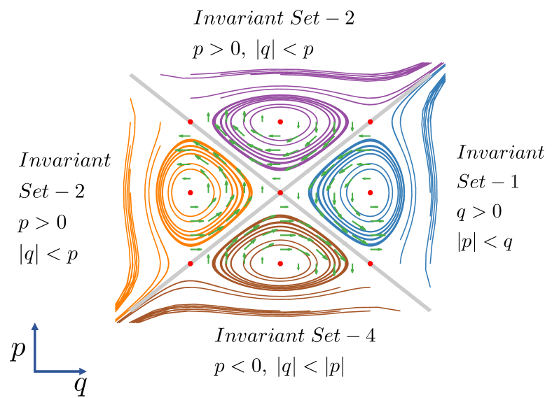
Figure 5: Phase portrait of the Hamiltonian system. Suppose if we start from the invariant set - 1 (IS-1), then the invariant set - 2 (IS-2) is obtained by $\gamma_{1}$-action on IS-1; invariant set - 3 (IS-3) is obtained by $\gamma_{2}$-action on IS-1; invariant set - 4 (IS-4) is obtained by $\gamma_{3}$-action on IS-1, which is same as $\gamma_{1}\gamma_{2}$-action on IS-1.

The local Koopman operators obtained using data from each of the invariant subspaces are

$${\bf K}_{IS-1}=\begin{pmatrix}0.955&0.486\\ -0.059&0.215\end{pmatrix};{\bf K}_{IS-2}=\begin{pmatrix}0.215&-0.059\\ 0.486&0.955\end{pmatrix}$$

$${\bf K}_{IS-3}=\begin{pmatrix}0.957&0.511\\ -0.061&0.214\end{pmatrix};{\bf K}_{IS-4}=\begin{pmatrix}0.214&-0.061\\ 0.511&0.957\end{pmatrix}$$

and it can be seen that ${\bf K}_{IS-2}=\gamma_{1}^{-1}{\bf K}_{IS-1}\gamma_{1}$. Similar relations are found to hold true for the other local Koopman operators. Hence if only one local Koopman operator is computed from data, all the other local Koopman operators can be computed using the relation of theorem 2, without using data from the other invariant subspaces and they are stitched together to obtain the global Koopman operator as described in Nandanoori et al. (2019).

6 Conclusions

In this paper, we developed Koopman operator theoretic based methods to study the global phase space in equivariant dynamical systems. In particular, we showed that the invariant subspaces are mapped to invariant subspaces and eigenspaces are left invariant under the group action of the symmetry group and established the properties of the Koopman operator for an equivariant dynamical system under group action. Assuming the knowledge of the type of symmetry in a dynamical system, it is shown that the global phase space can be studied based on data from any one invariant subspace only. The proposed framework is demonstrated on three different systems that possess various symmetries, such as reflective, rotational, or both. Future efforts focus on identifying the type of symmetries in a dynamical system, given the data for the global phase space.

References

- Budisic et al. (2012) Budisic, M., Mohr, R., and Mezic, I. (2012). Applied koopmanism. Chaos, 22, 047510–32.
- Chossat and Golubitsky (1988) Chossat, P. and Golubitsky, M. (1988). Symmetry-increasing bifurcation of chaotic attractors. Physica D: Nonlinear Phenomena, 32(3), 423–436.
- Dellnitz and Junge (1999) Dellnitz, M. and Junge, O. (1999). On the approximation of complicated dynamical behavior. SIAM Journal on Numerical Analysis, 36, 491–515.
- Dellnitz et al. (2005) Dellnitz, M., Junge, O., and et al (2005). Transport in dynamical astronomy and multibody problems. International Journal of Bifurcation and Chaos, 15, 699–727.
- Field (1970) Field, M. (1970). Equivariant dynamical systems. Bulletin of the American Mathematical Society, 76(6), 1314–1318.
- Field (1980) Field, M. (1980). Equivariant dynamical systems. Transactions of the American Mathematical Society, 259(1), 185–205.
- Froyland (2001) Froyland, G. (2001). Extracting dynamical behaviour via Markov models. In A. Mees (ed.), Nonlinear Dynamics and Statistics: Proceedings, Newton Institute, Cambridge, 1998, 283–324. Birkhauser.
- Gardner et al. (2000) Gardner, T.S., Cantor, C.R., and Collins, J.J. (2000). Construction of a genetic toggle switch in escherichia coli. Nature, 403(6767), 339.
- Golubitsky et al. (2012) Golubitsky, M., Stewart, I., and Schaeffer, D.G. (2012). Singularities and groups in bifurcation theory, volume 2. Springer Science & Business Media.
- Horn and Johnson (2012) Horn, R.A. and Johnson, C.R. (2012). Matrix analysis. Cambridge university press.
- Johnson and Yeung (2018) Johnson, C.A. and Yeung, E. (2018). A class of logistic functions for approximating state-inclusive koopman operators. In 2018 Annual American Control Conference (ACC), 4803–4810. IEEE.
- Junge and Osinga (2004) Junge, O. and Osinga, H. (2004). A set oriented approach to global optimal control. ESAIM: Control, Optimisation and Calculus of Variations, 10(2), 259–270.
- Lasota and Mackey (1994) Lasota, A. and Mackey, M.C. (1994). Chaos, Fractals, and Noise: Stochastic Aspects of Dynamics. Springer-Verlag, New York.
- Mauroy and Mezic (2013) Mauroy, A. and Mezic, I. (2013). A spectral operator-theoretic framework for global stability. In Proc. of IEEE Conference of Decision and Control. Florence, Italy.
- Mehta and Vaidya (2005) Mehta, P.G. and Vaidya, U. (2005). On stochastic analysis approaches for comparing dynamical systems. In Proceeding of IEEE Conference on Decision and Control, 8082–8087. Spain.
- Mesbahi et al. (2019) Mesbahi, A., Bu, J., and Mesbahi, M. (2019). On modal properties of the koopman operator for nonlinear systems with symmetry. In 2019 American Control Conference (ACC), 1918–1923. IEEE.
- Mezic and Banaszuk (2000) Mezic, I. and Banaszuk, A. (2000). Comparison of systems with complex behavior: spectral methods. In Proceedings of the 39th IEEE Conference on Decision and Control, 1224–1231.
- Mezić and Banaszuk (2004) Mezić, I. and Banaszuk, A. (2004). Comparison of systems with complex behavior. Physica D, 197, 101–133.
- Mezić (2005) Mezić, I. (2005). Spectral properties of dynamical systems, model reduction and decompositions. Nonlinear Dynamics, 41(1-3), 309–325.
- Nandanoori et al. (2019) Nandanoori, S.P., Sinha, S., and Yeung, E. (2019). Data-driven operator theoretic methods for global phase space learning. arXiv preprint arXiv:1910.03011.
- Petersen (1989) Petersen, K.E. (1989). Ergodic theory, volume 2. Cambridge University Press.
- Raghunathan and Vaidya (2014) Raghunathan, A. and Vaidya, U. (2014). Optimal stabilization using lyapunov measures. IEEE Transactions on Automatic Control, 59(5), 1316–1321.
- Salova et al. (2019) Salova, A., Emenheiser, J., Rupe, A., Crutchfield, J.P., and D’Souza, R.M. (2019). Koopman operator and its approximations for systems with symmetries. Chaos: An Interdisciplinary Journal of Nonlinear Science, 29(9), 093128.
- Schmid (2010) Schmid, P.J. (2010). Dynamic mode decomposition of numerical and experimental data. Journal of Fluid Mechanics, 656, 5–28.
- Sinha et al. (2018a) Sinha, S., Bowen, H., and Vaidya, U. (2018a). On robust computation of koopman operator and prediction in random dynamical systems. arXiv preprint arXiv:1803.08562.
- Sinha et al. (2018b) Sinha, S., Huang, B., and Vaidya, U. (2018b). Robust approximation of koopman operator and prediction in random dynamical systems. In 2018 Annual American Control Conference (ACC), 5491–5496. IEEE.
- Sinha et al. (2019a) Sinha, S., Nandanoori, S.P., and Yeung, E. (2019a). Online learning of dynamical systems: An operator theoretic approach. arXiv preprint arXiv:1909.12520.
- Sinha et al. (2019b) Sinha, S., Vaidya, U., and Yeung, E. (2019b). On computation of koopman operator from sparse data. In 2019 American Control Conference (ACC), 5519–5524. IEEE.
- Sparrow (2012) Sparrow, C. (2012). The Lorenz equations: bifurcations, chaos, and strange attractors, volume 41. Springer Science & Business Media.
- Surana and Banaszuk (2016) Surana, A. and Banaszuk, A. (2016). Linear observer synthesis for nonlinear systems using koopman operator framework. IFAC-PapersOnLine, 49(18), 716–723.
- Susuki and Mezic (2011) Susuki, Y. and Mezic, I. (2011). Nonlinear koopman modes and coherency identification of coupled swing dynamics. IEEE Transactions on Power Systems, 26(4), 1894–1904.
- Vaidya and Mehta (2008) Vaidya, U. and Mehta, P.G. (2008). Lyapunov measure for almost everywhere stability. IEEE Transactions on Automatic Control, 53(1), 307–323.
- Williams et al. (2015) Williams, M.O., Kevrekidis, I.G., and Rowley, C.W. (2015). A data–driven approximation of the koopman operator: Extending dynamic mode decomposition. Journal of Nonlinear Science, 25(6), 1307–1346.
- Yeung et al. (2017) Yeung, E., Kundu, S., and Hodas, N. (2017). Learning deep neural network representations for koopman operators of nonlinear dynamical systems. arXiv preprint arXiv:1708.06850.
- Yeung et al. (2018) Yeung, E., Liu, Z., and Hodas, N.O. (2018). A koopman operator approach for computing and balancing gramians for discrete time nonlinear systems. In 2018 Annual American Control Conference (ACC), 337–344. IEEE.