On the FRB luminosity function – II. Event rate density

Abstract

The luminosity function of Fast Radio Bursts (FRBs), defined as the event rate per unit cosmic co-moving volume per unit luminosity, may help to reveal the possible origins of FRBs and design the optimal searching strategy. With the Bayesian modelling, we measure the FRB luminosity function using 46 known FRBs. Our Bayesian framework self-consistently models the selection effects, including the survey sensitivity, the telescope beam response, and the electron distributions from Milky Way / the host galaxy / local environment of FRBs. Different from the previous companion paper, we pay attention to the FRB event rate density and model the event counts of FRB surveys based on the Poisson statistics. Assuming a Schechter luminosity function form, we infer (at the 95% confidence level) that the characteristic FRB event rate density at the upper cut-off luminosity $L^{*}=2.9_{-1.7}^{+11.9}\times 10^{44}\,\mathrm{erg}\,\mathrm{s}^{-1}$ is $\phi^{*}=339_{-313}^{+1074}\,\mathrm{Gpc}^{-3}\,\mathrm{yr}^{-1}$, the power-law index is $\alpha=-1.79_{-0.35}^{+0.31}$, and the lower cut-off luminosity is $L_{0}\leq 9.1\times 10^{41}\,\mathrm{erg}\,\mathrm{s}^{-1}$. The event rate density of FRBs is found to be $3.5_{-2.4}^{+5.7}\times 10^{4}\,\mathrm{Gpc}^{-3}\,\mathrm{yr}^{-1}$ above $10^{42}\,\mathrm{erg}\,\mathrm{s}^{-1}$, $5.0_{-2.3}^{+3.2}\times 10^{3}\,\mathrm{Gpc}^{-3}\,\mathrm{yr}^{-1}$ above $10^{43}\,\mathrm{erg}\,\mathrm{s}^{-1}$ , and $3.7_{-2.0}^{+3.5}\times 10^{2}\,\mathrm{Gpc}^{-3}\,\mathrm{yr}^{-1}$ above $10^{44}\,\mathrm{erg}\,\mathrm{s}^{-1}$. As a result, we find that, for searches conducted at 1.4 GHz, the optimal diameter of single-dish radio telescopes to detect FRBs is 30–40 m. The possible astrophysical implications of the measured event rate density are also discussed in the current paper.

1 Introduction

The origin of Fast Radio Bursts (FRBs) is still unknown, in spite of the fact that the initial discovery was made a decade ago (Lorimer et al., 2007). Observationally, FRBs are radio flashes that last for a few milliseconds and exhibit prominent dispersion with peak flux densities ranging from $\sim$0.05 Jy to $\sim$150 Jy (see FRB catalogue, FRBCAT; Petroff et al., 2016). Due to the limited beam size of traditional single-dish radio telescopes, the detection rate was typically low (Lawrence et al., 2017) and the total number of FRBs was around 30 by 2018. The situation changed dramatically in recent years, thanks to the deployment of telescope arrays with large fields of view (FoV), e.g. ASKAP with $\mathrm{FoV}=160\,\mathrm{deg}^{2}$ (Bannister et al., 2017) and CHIME with $\mathrm{FoV}>200\,\mathrm{deg}^{2}$ (CHIME/FRB Collaboration et al., 2018). Those new facilities have greatly boosted the annual detection rate of FRBs. Up to 2020, the number of verified FRB sources has been over 100.

With the growing number of detected FRBs, one can perform statistical studies of the FRB population. The studies carried out so far cover the investigations for source count—flux ($\log N(\geq F)-\log F$) relation (Vedantham et al., 2016; Macquart & Ekers, 2018; Golpayegani et al., 2019), $V/V_{\rm max}$ test (Oppermann et al., 2016; Locatelli et al., 2019), FRB event rate distribution (Bera et al., 2016; Lawrence et al., 2017), repetition properties (Connor et al., 2016b; Connor & Petroff, 2018; Caleb et al., 2019), and volumetric event rate (Deng et al., 2019; James, 2019; Lu & Piro, 2019). All the above analyses can be, in principal, derived from the FRB luminosity function (LF), i.e. the event rate per unit co-moving volume per unit luminosity scale. The LF characterises the basic properties of FRB population, i.e. spatial number density, occurrence frequency, and luminosity distribution. If the LF is known, one can directly compute the above mentioned statistics and compare them to observations. Furthermore, one can calculate the detection rate of telescopes by integrating the LF above the telescope thresholds. This can be used to design the FRB searching plan in the future. The FRB event rate densities at different luminosity ranges may provide hints in investigating their origins and possible progenitors (e.g. Platts et al., 2019).

In our previous work (Luo et al., 2018, ; hereafter L18), we measured the normalised FRB LF (i.e., probability density of FRBs per unit luminosity interval) using a sample of 33 FRBs with Bayesian method. L18 investigated the relative power output of FRB population in different luminosity bins, but did not address how frequently FRB events occur per unit time per unit volume in different luminosity ranges. In the current paper, we aims to measure the true LF, i.e., number of FRBs per co-moving volume per unit time per luminosity scale.

The major differences between this paper and L18 are:

• L18 did not take into account the exact survey information, such as survey time, field of view, detection number. Those data are used in this paper.

• No modelling for event occurrence was carried out in L18, whereas we consider both a random process of event counts and the FRB duration distribution in this paper.

• The sample used in this paper, among which there are many ASKAP detections, is larger than that of L18.

The structure of this paper is organised as follows. In Section 2, we extend our previous model to include the epochs of FRB events using the Poisson Process. The verification of the Bayesian inference algorithm using the mock data is also made there. The results of the inference to the observed FRB sample is shown in Section 3. Relevant discussion and conclusions are made in Section 4.

2 Bayesian Framework

As described in L18, throughout this paper we make extensive use of Bayes’ theorem, which relates the probability density functions (PDFs) involving data ($\bf X$) to parameters ($\bf\Theta$) as follows,

$$P({\bf\Theta|X})=\frac{P({\bf\Theta})P({\bf X|\Theta})}{P({\bf X})}\,,$$ (1)

where the symbol $|$ denotes a conditional probability. The likelihood function, $P({\bf X|\Theta})$, is the PDF of the data given the model parameters. $P(\bf\Theta|X)$ is the posterior PDF, i.e. the PDF of the parameters given the data set. The Bayesian evidence is defined as

$$P({\bf X})=\int P({\bf\Theta})P({\bf X|\Theta})\,\mathrm{d}{\boldsymbol{{\Theta}}}\,.$$ (2)

Finally, the prior PDF $P(\bf\Theta)$ describes a priori information about the model.

2.1 Observations

For the application of Bayesian inference in the current work, the data ${\boldsymbol{{X}}}$ are the observables from FRB observations, and the parameters ${\boldsymbol{{\Theta}}}$ are the theoretical parameters we want to measure. The observables used in the current work are, peak flux density ($S_{\rm peak}$), extra-galactic dispersion measure ($\mathrm{DM}_{\rm E}$), pulse width ($w$), number of FRB detected in a given survey ($N$), time length of survey ($t_{\rm svy}$), and FoV of survey ($\Omega$). Here $\mathrm{DM}_{\rm E}$ is obtained by subtracting the Galactic contribution using the YMW16 model (Yao et al., 2017). With the exception of $t_{\rm svy}$, $N$ and $\Omega$, which are new additions, these parameters had been discussed in L18.

The data we use come from a variety of pulsar surveys carried out around 1 GHz: the Parkes Magellanic Cloud Pulsar Survey ((PKS-MC; Lorimer et al., 2007; Zhang et al., 2019); the High Time Resolution Universe (HTRU; Thornton et al., 2013; Champion et al., 2016; Ravi et al., 2015; Petroff et al., 2015a, 2017); the Survey for Pulsars and Extragalactic Radio Bursts (SUPERB; Keane et al., 2016; Ravi et al., 2016; Bhandari et al., 2018a), Pulsar Arecibo L-band Feed Array (PALFA; Spitler et al., 2014); Green Bank Telescope Intensity Mapping (GBTIM; Masui et al., 2015); UTMOST Southern Sky (UTMOST-SS; Caleb et al., 2017)) and the Commensal Real-time ASKAP Fast Transients (CRAFT; Shannon et al., 2018). We do not include the CHIME discoveries, since we focus on the FRB LF whose radio emission is around 1 GHz. To include 400 MHz to 800 MHz band of CHIME, the detailed modelling of spectrum is required, which we defer to a future paper. The properties of these 7 surveys and 46 FRBs related to the current work are listed in Table 1 and Table 2, respectively.

We include the repeating FRB 121102 in our sample. Considering we are studying on the FRB occurrence rate in this paper, there is a subtle difference between using the initial discovery and later follow-ups. For the initial discovery, one did not know the FRB position, FoV, the telescope gain and the observing duration that determine the searching volume. By contrast, for later follow-up observations, one already knew the source position so that the observers can design the telescope gain (by choosing the right telescope) and the observation time to monitor the target. For the purpose of deriving the true FRB LF, we only use the information of initial discovery to avoid complicated selection effects introduced by follow-up observations. An underlying assumption is that we regard the repeating and non-repeating FRBs as a uniform population.

Table 1: The known FRB surveys

Survey	$N_{\rm FRB}$a	$\Omega$b	$t_{\rm svy}$c	$G$d	$T_{\rm sys}$e	BWf	S/N0g	$N_{\mathrm{p}}$h	Ref.i
		($\mathrm{deg}^{2}$)	(hr)	(K/Jy)	(K)	(MHz)
PKS-MC	2	0.556	490.5	0.69	28	288	7	2	[1]
HTRU&SUPERB	19	0.556	7357	0.69	28	338	10	2	[2]
PALFA	1	0.024	11503.3	0.7j	30	322	7	2	[1]
GBTIM	1	0.055	660	2.0	25	200	8	2	[3]
UTMOST-SS	3	9	4320	3.0	400	16	10	1	[4]
CRAFT	20	160	3187.5	0.05	100	336	10	2	[5]

• (a) Detection number. (b) Field of view in units of $\mathrm{deg}^{2}$. (c) Survey time in units of hour. (d) Telescope gain in units of K/Jy. (e) System temperature in units of K. (f) Bandwidth in units of MHz. (g) Threshold of signal-to-noise ratio. (h) Polarization channel number.

• (i) The references are: [1] Lawrence et al. (2017); [2] Bhandari et al. (2018a); [3] Connor et al. (2016c); [4] Caleb et al. (2017); [5] Shannon et al. (2018);

• (j) The Arecibo FRB (FRB 121102) was probably detected in the sidelobe of 7-beam receiver, the gain of sidelobe is about 0.7 K/Jy (Spitler et al., 2014).

Table 2: The parameters of FRB sample we use

FRB	$S_{\mathrm{peak}}$a	$w$b	$F$c	DMd	$\mathrm{DM}_{\rm MW}$e	$\mathrm{DM}_{\rm MW}$f	Survey	Ref.g
	(Jy)	(ms)	(Jy ms)	($\mathrm{cm}^{-3}\,\mathrm{pc}$)	($\mathrm{cm}^{-3}\,\mathrm{pc}$)	($\mathrm{cm}^{-3}\,\mathrm{pc}$)
010312	$0.25$	$24.3$	$6.10$	$1187.0$	$51.0$	$67.0$	PKS-MC	[1]
010724	$30.0$	$5.0$	$150.0$	$375.0$	$44.6$	$94.0$	PKS-MC	[2]
090625	$1.14$	$1.92$	$2.19$	$899.5$	$31.7$	$25.5$	HTRU	[3]
110214	$27.0$	$1.9$	$54.0$	$168.8$	$31.1$	$21.1$	HTRU	[4]
110220	$1.3$	$5.6$	$7.28$	$944.4$	$34.8$	$24.1$	HTRU	[5]
110523	$0.6$	$1.73$	$1.04$	$623.3$	$43.5$	$33.0$	GBTIM	[6]
110626	$0.4$	$1.4$	$0.56$	$723.0$	$47.5$	$33.6$	HTRU	[5]
110703	$0.5$	$4.3$	$2.15$	$1103.6$	$32.3$	$23.1$	HTRU	[5]
120127	$0.5$	$1.1$	$0.55$	$553.3$	$31.8$	$20.6$	HTRU	[5]
121002	$0.43$	$5.44$	$2.34$	$1629.2$	$74.3$	$60.5$	HTRU	[3]
121102	$0.4$	$3.0$	$1.2$	$557.0$	$188.0$	$287.1$	PALFA	[7]
130626	$0.74$	$1.98$	$1.47$	$952.4$	$66.9$	$65.1$	HTRU	[3]
130628	$1.91$	$0.64$	$1.22$	$469.9$	$52.6$	$47.0$	HTRU	[3]
130729	$0.22$	$15.61$	$3.43$	$861.0$	$31.0$	$25.4$	HTRU	[3]
131104	$1.12$	$2.08$	$2.33$	$779.0$	$71.1$	$220.2$	HTRU	[8]
140514	$0.47$	$2.8$	$1.32$	$562.7$	$34.9$	$24.2$	HTRU	[9]
150215	$0.7$	$2.8$	$1.96$	$1105.6$	$427.2$	$296.4$	HTRU	[10]
150418	$2.2$	$0.8$	$1.76$	$776.2$	$188.5$	$325.5$	SUPERB	[11]
150610	$0.7$	$2.0$	$1.3$	$1593.9$	$122.0$	$122.9$	SUPERB	[12]
150807	$128.0$	$0.35$	$44.8$	$266.5$	$36.9$	$25.1$	SUPERB	[13]
151206	$0.3$	$3.0$	$0.9$	$1909.8$	$160.0$	$161.0$	SUPERB	[12]
151230	$0.42$	$4.4$	$1.9$	$960.4$	$38.0$	$37.8$	SUPERB	[12]
160102	$0.5$	$3.4$	$1.8$	$2596.1$	$13.0$	$21.8$	SUPERB	[12]
160317	$3.0$	$21.0$	$63.0$	$1165.0$	$319.6$	$394.6$	UTMOST-SS	[14]
160410	$7.0$	$4.0$	$28.0$	$278.0$	$57.7$	$56.7$	UTMOST-SS	[14]
160608	$4.3$	$9.0$	$38.7$	$682.0$	$238.3$	$310.3$	UTMOST-SS	[14]
170107	$22.3$	$2.6$	$57.98$	$609.5$	$35.0$	$25.2$	CRAFT	[15]
170416	$19.4$	$5.0$	$97.0$	$523.2$	$40.0$	$27.5$	CRAFT	[15]
170428	$7.7$	$4.4$	$34.0$	$991.7$	$40.0$	$27.4$	CRAFT	[15]
170707	$14.8$	$3.5$	$52.0$	$235.2$	$36.0$	$26.9$	CRAFT	[15]
170712	$37.8$	$1.4$	$53.0$	$312.8$	$38.0$	$26.5$	CRAFT	[15]
170906	$29.6$	$2.5$	$74.0$	$390.3$	$39.0$	$26.6$	CRAFT	[15]
171003	$40.5$	$2.0$	$81.0$	$463.2$	$40.0$	$35.4$	CRAFT	[15]
171004	$22.0$	$2.0$	$44.0$	$304.0$	$38.0$	$33.0$	CRAFT	[15]
171019	$40.5$	$5.4$	$219.0$	$460.8$	$37.0$	$26.3$	CRAFT	[15]
171020	$117.6$	$1.7$	$200.0$	$114.1$	$38.0$	$25.8$	CRAFT	[15]
171116	$19.6$	$3.2$	$63.0$	$618.5$	$36.0$	$37.5$	CRAFT	[15]
171213	$88.6$	$1.5$	$133.0$	$158.6$	$36.0$	$33.8$	CRAFT	[15]
171216	$21.0$	$1.9$	$40.0$	$203.1$	$37.0$	$28.7$	CRAFT	[15]
180110	$128.1$	$3.2$	$420.0$	$715.7$	$38.0$	$26.1$	CRAFT	[15]
180119	$40.7$	$2.7$	$110.0$	$402.7$	$36.0$	$37.9$	CRAFT	[15]
180128.0	$17.5$	$2.9$	$51.0$	$441.4$	$32.0$	$26.6$	CRAFT	[15]
180128.2	$28.7$	$2.3$	$66.0$	$495.9$	$40.0$	$28.3$	CRAFT	[15]
180130	$23.1$	$4.1$	$95.0$	$343.5$	$39.0$	$26.1$	CRAFT	[15]
180131	$22.2$	$4.5$	$100.0$	$657.7$	$40.0$	$26.9$	CRAFT	[15]
180212	$53.0$	$1.81$	$96.0$	$167.5$	$33.0$	$27.8$	CRAFT	[15]

• From left to right, for each FRB, we list (a) peak flux density, $S_{\rm peak}$; (b) pulse width, $w$ (with scattering removed); (c) fluence (pulse engergy), $F$; (d) dispersion measure, DM; (e) Galactic DM calculated by the NE2001 model (Cordes & Lazio, 2002); (f) Galactic DM calculated by the YMW16 model (Yao et al., 2017);

• (g) The references are: [1] Zhang et al. (2019); [2] Lorimer et al. (2007); [3] Champion et al. (2016); [4] Petroff et al. (2019); [5] Thornton et al. (2013); [6] Masui et al. (2015); [7] Spitler et al. (2014); [8] Ravi et al. (2015); [9] Petroff et al. (2015a); [10] Petroff et al. (2017); [11] Keane et al. (2016); [12] Bhandari et al. (2018a); [13] Ravi et al. (2016); [14] Caleb et al. (2016); [15] Shannon et al. (2018).

2.2 Likelihood function

The likelihood function used in Bayesian inference is the probability distribution function of observables given the model parameters. The likelihood we used is an extension of the work in L18, where more details of likelihood construction are explained. Here we present a brief introduction and refer the readers to L18 for further details. Basically, we should make three assumptions for the distribution functions of luminosity ($L$), intrinsic duration ($w_{\mathrm{i}}$) and random process of FRB events. These are as follows:

(i) Following L18, the FRB luminosity is isotropic and its distribution follows a Schechter function. Due to the limited FRB number, we neglect the cosmic evolution of FRB LF, with the caveat that the star formation rate evolves significantly at low redshifts ($z\leq 1$). There are two reasons why we adopt the Schechter function: (1) The Schechter function has a power-law shape and a smooth exponential cut-off in the high luminosity end, which makes it easy to compare with the other results usually assuming a power-law LF; (2) The function is widely used for extragalactic objects, such as galaxies, quasars, gamma-ray bursts, etc. Similarly, it is rather straightforward to compare the LF of FRBs with the other astronomical objects.

(ii) The FRB intrinsic duration distribution is log-normal in form (Connor, 2019) and independent of FRB LF. This is a new assumption introduced compared to L18. On one hand, the duration distribution is required, since we now need to compute the detection selection effect of FRBs in a given survey. On the other hand, measuring the duration distribution may be useful for progenitor studies.

(iii) The time of arrival for FRBs of a given survey follows the Poisson process, a consequence if FRBs are independent and stationary in a unit comoving volume.

(iv) The FRB true position is randomly and uniformly located in the telescope beam.

In addition, to derive the joint distribution function, we make four extra assumptions for independence:

(v) The cosmic spatial distribution of FRBs can be treated as homogeneous in comoving volume for such a limited sample.

(vi) The FRB LF is independent of FRB host galaxies.

(vii) The source DM contribution is independent of the host-galaxy DM.

The general Bayesian framework shown in the current paper, however, does not depend on the assumption i) to iv), i.e. one can replace the corresponding models to perform inference in a similar fashion.

Under the seven assumptions above, we can write the joint distribution function for the quantities {$\log L$, $\log w_{\mathrm{i}}$, $N$, $z$, $\mathrm{DM}_{\rm host}$, $\mathrm{DM}_{\rm src}$, $\log\epsilon$}, which are logarithmic luminosities, logarithmic pulse widths, number of FRBs in a given survey, redshifts of FRBs, host galaxg DMs, local DM contributions, and beam responses. We refer the readers with interests on this derivation to L18 for the details. Due to the independence assumed above, the likelihood is the multiplication of individual likelihood of each observables, i.e.

$$f(\log L,\log w_{\mathrm{i}},N,z,\mathrm{DM}_{\rm host},\mathrm{DM}_{\rm src},\log\epsilon)$$ (3)

$$={}\phi(\log L)\,f_{\mathrm{w}}(\log w_{\mathrm{i}})\,P(N)\,f_{z}(z)\,f_{\cal D}(\mathrm{DM}_{\rm host}|z)\,f_{\mathrm{s}}(\mathrm{DM}_{\rm src})\,f_{\mathrm{\epsilon}}(\log\epsilon)\,.$$

Here $\phi(\log L)$ is the LF (see Section 2.2.1 for details), $f_{\mathrm{w}}(\log w_{\mathrm{i}})$ is the FRB intrinsic duration distribution (Section 2.2.2), $P(N)$ is the Poisson distribution describing the number of events (Section 2.2.7), $f_{z}(z)$ is the FRB cosmic spatial distribution function (Section 2.2.3), $f_{\cal D}(\mathrm{DM}_{\rm host}|z)$ is the host DM distribution function at redshift of $z$ (Section 2.2.4), $f_{\mathrm{s}}(\mathrm{DM}_{\rm src})$ is the source DM distribution function (Section 2.2.5) and $f_{\mathrm{\epsilon}}(\log\epsilon)$ is the beam response distribution function (Section 2.2.6).

We can compute the likelihood function for those observables {$S_{\rm peak}$, $w$, $\mathrm{DM}_{\rm E}$, $N$} from Equation (3). The first step is to transform the variables using the Jacobian transformation. As shown in Appendix A, this leads to

$$f(\log S,\log w_{\mathrm{o}},N,\mathrm{DM}_{\rm E},z,\mathrm{DM}_{\rm src},\log\epsilon)$$ (4)

$$={}\phi(\log L)f_{\mathrm{w}}(\log w_{\mathrm{i}})P(N)f_{\cal D}(\mathrm{DM}_{\rm host}|z)f_{z}(z)f_{\mathrm{s}}(\mathrm{DM}_{\rm src})$$

$$\quad\cdot f_{\mathrm{\epsilon}}(\log\epsilon)(1+z)\,.$$

Since redshift ($z$), FRB local DM ($\mathrm{DM}_{\rm src}$), and beam response ($\epsilon$) are not direct observables, we marginalise them by integrating Equation (3). The reduced likelihood becomes

$$\mathcal{L}(\log S,w_{\mathrm{o}},N,\mathrm{DM}_{\rm E}) =\prod_{j=1}^{M}\mathcal{L}_{j}(N_{j})\cdot\prod_{k=1}^{N}f(\log S_{k},\,\log w_{\mathrm{o},\,k},\,\mathrm{DM}_{\mathrm{E},\,k})$$ (5)

$$=\frac{\prod_{j=1}^{M}(\rho_{j}\Omega_{j}t_{j})^{N_{j}}\cdot\exp\left(-\sum_{j=1}^{M}\rho_{j}\Omega_{j}t_{j}\right)}{\prod_{j=1}^{M}N_{j}!}$$

$$\quad\cdot\prod_{k=1}^{N}f(\log S_{k},\,\log w_{\mathrm{o},\,k},\,\mathrm{DM}_{\mathrm{E},\,k})\,,$$

where the subscript $j$ refers to the surveys and $k$ refers to the FRBs. $\rho_{j}$ is the event rate of the $j$-th survey, $\Omega_{j}$ is the FoV of the survey, $t_{j}$ is its observational time, and $N_{j}$ is the number of FRBs detected in the $j$-th survey. The summation of all survey detections $N=\sum_{j=1}^{M}N_{j}$.

The function

$$f(\log S_{k},\,\log w_{\mathrm{o},\,k},\,\mathrm{DM}_{\mathrm{E},\,k}) =\frac{1}{N_{\mathrm{f}}}\int_{0}^{\infty}I(\log L)\,f_{\mathrm{w}}\left(\frac{w_{\mathrm{o},\,k}}{1+z}\right)f_{z}(z)\,$$ (6)

$$\quad I(\mathrm{DM}_{\mathrm{E},\,k},\,z)\,(1+z)\,\mathrm{d}z\,,$$

with

$$I(\log L)=\int\phi(\log L)f_{\mathrm{\epsilon}}(\log\epsilon)\,\mathrm{d}\log\epsilon\,.$$ (7)

and

$$I(\mathrm{DM}_{\mathrm{E},\,k},\,z)=\int_{0}^{\max(\mathrm{DM}_{\rm s})}f_{\cal D}(\mathrm{DM}_{\rm host}|z)f_{\mathrm{s}}(\mathrm{DM}_{\rm src})\,\mathrm{d}\mathrm{DM}_{\rm src}\,.$$ (8)

$N_{\mathrm{f}}$ is the normalisation factor defined as

$$N_{\mathrm{f}} =\int_{\log S_{\rm min}(w_{\mathrm{o}})}^{\infty}\,\mathrm{d}\log S\int\int\int f(\log S,\log w_{\mathrm{o}},\mathrm{DM}_{\rm E},z)\,$$ (9)

$$\quad\cdot\mathrm{d}\log w_{\mathrm{o}}\,\mathrm{d}\mathrm{DM}_{\rm E}\,\mathrm{d}z\,,$$

where the minimum detectable flux density

$$S_{\mathrm{min}}(w_{\mathrm{o}})=\frac{\mathrm{S/N}_{0}\ T_{\mathrm{sys}}}{G\sqrt{N_{\mathrm{p}}\,\mathrm{BW}\,w_{\mathrm{o}}}}\,.$$ (10)

Here $\mathrm{S/N}_{0}$ is the signal-to-noise ratio (S/N) threshold for detections in the surveys, $T_{\rm sys}$ is the system temperature, $G$ is the telescope gain, $N_{\mathrm{p}}$ is the number of polarization summed, and ${\rm BW}$ is the bandwidth.

In the following subsections (from Section 2.2.1 to Section 2.2.7), we explain the distribution functions appeard in the above equations individually.

2.2.1 The form of FRB LF

As in L18, we assume a Schechter LF (Schechter, 1976) in which the volumetric event rate density

$$\phi(L)\,\mathrm{d}L=\phi^{*}\left(\frac{L}{L^{*}}\right)^{\alpha}e^{-\frac{L}{L^{*}}}\,\mathrm{d}\left(\frac{L}{L^{*}}\right)\,,$$ (11)

where $\phi^{*}$ is the characteristic volumetric density of event rate in units of $\mathrm{Gpc}^{-3}\,\mathrm{yr}^{-1}$, $\alpha$ is the power-law index, and $L^{*}$ is the upper cut-off luminosity. In logarithmic scale, the form of LF is

$$\phi(\log L)\,\mathrm{d}\log L=\ln 10\,\phi^{*}\left(\frac{L}{L^{*}}\right)^{\alpha+1}e^{-\frac{L}{L^{*}}}\,\mathrm{d}\log L\,.$$ (12)

2.2.2 The intrinsic duration distribution

As shown in Equation (10), the selection threshold depends on the FRB duration. We need intrinsic duration distribution to compute the selection biases of FRBs with different observed widths. We assume that the intrinsic FRB width distribution is log-normal in form (see, e.g., Connor, 2019) that

$$f_{\mathrm{w}}(\log w_{\mathrm{i}})=\frac{1}{\sqrt{2\pi\sigma_{\rm w}^{2}}}\exp\left[-\frac{(\log w_{\mathrm{i}}-\mu_{\rm w})^{2}}{2\sigma_{\rm w}^{2}}\right],$$ (13)

where $\mu_{\rm w}$ and $\sigma_{\rm w}$ are, respectively, the mean and standard deviation of this distribution.

2.2.3 The cosmic spatial distribution

The FRB spatial distribution is assumed to be uniform in co-moving volume, that is

$$f_{z}(z)=\frac{\mathrm{d}V}{\mathrm{d}z}=\frac{cr^{2}(z)}{H_{0}E(z)}\,,$$ (14)

where $c$ is the speed of light, $r$ is the comoving distance, $H_{0}$ is the Hubble constant and $E(z)$ is the logarithmic time derivative of the cosmic scale factor in a flat $\Lambda$CDM universe, i.e.

$$E(z)=\sqrt{\Omega_{\rm m}(1+z)^{3}+\Omega_{\Lambda}}\,.$$ (15)

The cosmology model we use here are from Planck observations, i.e. we take $H_{0}=67.8\,{\rm km\,s^{-1}\,Mpc^{-1}}$, $\Omega_{\rm m}=0.308$ and $\Omega_{\Lambda}=0.692$ (Planck Collaboration et al., 2016).

2.2.4 The DM distribution of host galaxies

As shown in L18, the distribution function for $\mathrm{DM}_{\rm host}$ evolves as a function of redshift. L18 showed that

$$f_{\cal D}(\mathrm{DM}_{\rm host}|z)=\sqrt{\frac{\mathrm{SFR}(0)}{\mathrm{SFR}(z)}}f_{\cal D}\left[\mathrm{DM}_{\rm host}\sqrt{\frac{\mathrm{SFR}(0)}{\mathrm{SFR}(z)}}\right]\,,$$ (16)

where $\mathrm{SFR}(z)$ is the cosmic star formation rate at redshift of $z$. The function $f_{\cal D}(\mathrm{DM}_{\rm host,0})$ was computed numerically and approximated using multiple Gaussian functions in L18, i.e. we take

$$f_{\cal D}(\mathrm{DM}_{\rm host,0})\,\mathrm{d}\mathrm{DM}_{\rm host,0}=\sum_{i=1}^{2}a_{i}e^{-\left(\frac{\log\mathrm{DM}_{\rm host,0}-b_{i}}{c_{i}}\right)^{2}}\,\mathrm{d}\mathrm{DM}_{\rm host,0}\,.$$ (17)

As shown in L18, the difference is not substantial when using different DM models for host galaxies. To reduce the length of the current paper, we merely use the model ‘ALG(YMW16)" in L18, i.e. model $\mathrm{DM}_{\rm host,0}$ for all types of galaxies with the YMW16 templates.

2.2.5 The local DM from FRB source

Following L18, due to lack of knowledge on FRB progenitors, we take the least-informative assumption that $\mathrm{DM}_{\rm src}$ follows a uniform distribution in a rather wider range from 0 to 50 $\mathrm{cm}^{-3}\,\mathrm{pc}$, i.e.

$$f_{\mathrm{s}}(\mathrm{DM}_{\rm src})=\begin{cases}1/50\hskip 30.00005pt0<\mathrm{DM}_{\rm src}<50\,\mathrm{cm}^{-3}\,\mathrm{pc}\,,\\ 0\hskip 105.00015pt\textrm{Otherwise.}\end{cases}$$ (18)

2.2.6 The telescope beam response

The main beam response distribution function we use here is a Gaussian beam (see, e.g., Born & Wolf, 1999). We define the ratio of the observed flux ($S_{\rm obs}$) to the intrinsic flux ($S_{\rm src}$) for an FRB as

$$\epsilon\equiv\frac{S_{\rm obs}}{S_{\rm src}}=e^{-4\ln 2\left(\frac{\theta}{\theta_{\rm b}}\right)^{2}}\,,$$ (19)

where $\theta$ is the angular distance between the true position of FRB and the beam centre, $\theta_{\rm b}$ is the full-width-half-maximum (FWHM) beam size, i.e. $\epsilon=0.5$ for $\theta=\theta_{\rm b}/2$.

Adopting a uniform distribution per solid angle for the source position inside the FWHM of beam, one will have (L18)

$$f_{\mathrm{\epsilon}}(\log\epsilon)=\begin{cases}1/\log 2\hskip 50.00008pt\textrm{Inside}\,,\\ 0\hskip 68.00012pt\textrm{Outside}\,.\end{cases}$$ (20)

2.2.7 Event counts likelihood

In L18, the parameter that contains the units of event rate ($\phi^{*}$) is canceled, when the marginalisation and normalisation were done (also see Equation (6)). In this work, as we model the random process of event occurrence, $\phi^{*}$ is kept in the event counts likelihood.

We assume the number of independent FRBs events that occur in a certain time interval for a given survey follows the Poisson distribution. This requires that the FRB event rate is stationary, and the bursts are independent (in a probabilistic sense) with each other. Assuming Poisson statistics, the probability of detecting $N$ FRB events in a particular survey,

$$P(N)=\frac{(\rho\Omega t)^{N}e^{-\rho\Omega t}}{N!},$$ (21)

where $\rho$ is the event rate per solid angle, namely surface event rate. $\Omega$ is the field of view and $t$ is the survey time. As shown in Appendix B, integrating the LF, we find that

$$\rho=\int_{0}^{\infty}\frac{1}{1+z}\frac{r(z)^{2}}{H(z)}\mathrm{d}z\int_{\log L_{\mathrm{min}}(w_{\mathrm{o}})}^{\infty}I(\log L)\,\mathrm{d}\log L$$ (22)

where $H(z)$ is the Hubble parameter, $r$ is the comoving distance. The low limit of integrating the LF, i.e. the minimum observed luminosity, is $L_{\mathrm{min}}(w_{\mathrm{o}})=\max\left[L_{0},L_{\mathrm{thre}}(w_{\mathrm{o}})\right]$. Here, $L_{0}$ is the intrinsic lower cut-off of LF and the survey detection threshold

$$L_{\mathrm{thre}}(w_{\mathrm{o}})\equiv 4\pi d_{\rm L}^{2}\Delta\nu_{0}S_{\mathrm{min}}\,,$$ (23)

where $d_{\rm L}$ is the luminosity distance, $\Delta\nu_{0}$ is the intrinsic spectrum width, and $S_{\rm min}$ is the flux detection threshold as defined in Equation (10).

According to Equation (10), $S_{\rm min}$ depends on the observed pulse width $w_{\mathrm{o}}$. Hence, the event rate seen by observer (i.e. event rate per solid angle $\rho$) depends on $w_{\mathrm{o}}$ as well. As proven in Appendix C, the event rate for all FRBs is the summation of event rates of individual ones. As the pulse width is a continuous random variable, the summation becomes an integration weighted by the width distribution function, i.e.

$$\rho =\int_{0}^{\infty}\frac{1}{1+z}\frac{r(z)^{2}}{H(z)}\mathrm{d}z\int f_{\mathrm{w}}(\log w_{\mathrm{i}})\,\mathrm{d}\log w_{\mathrm{i}}$$ (24)

$$\quad\cdot\int_{\log L_{\mathrm{min}}(w_{\mathrm{o}})}^{\infty}I(\log L)\,\mathrm{d}\log L\,.$$

For the $j$-th survey, the likelihood of detecting $N_{j}$ FRBs is

$$\mathcal{L}_{j}(N_{j})=\frac{(\rho_{j}\Omega_{j}t_{j})^{N_{j}}e^{-\rho_{j}\Omega_{j}t_{j}}}{N_{j}!}\,,$$ (25)

where $\rho_{j}$ is the apparent event rate per solid angle for this survey, which can be calculated using Equation (24).

2.3 Inference algorithm and its verification

With the likelihood function Equation (5), we can perform parameter inference using standard Bayesian sampling algorithm. Similar to L18, we use the multinest algorithm developed by Feroz et al. (2009) to perform the parameter sampling and inference.

We use the simulated data to verify our method. The simulated data is generated using Monte-Carlo simulation, where the recipe is summarised as following

1) Generate the FRB luminosities $L$ according to the Schechter function (Equation (11));

2) Generate the intrinsic FRB pulse widths $w_{\mathrm{i}}$ according to Equation (13);

3) Generate FRB redshifts $z$ according to the FRB cosmic spatial distribution (Equation (14)) and calculate the observed pulse width using $w_{\mathrm{o}}=w_{\mathrm{i}}(1+z)$;

4) Generate the host galaxy DMs ($\mathrm{DM}_{\rm host}$) at the redshift $z$ using the DM distribution function mentioned in Section 2.2.4;

5) Generate the FRB local DMs according to Equation (18);

6) Draw a sample of FRB positions in the beam according to Equation (19);

7) Based on the above parameters, calculate the observed FRB flux densities and extragalactic DMs;

8) Select the FRBs above the flux threshold $S_{\rm min}$ for detections.

9) Simulate the FRB arrival times according to the Poisson distribution.

We perform two simulations with two sets of input parameters. Each simulation produces 100 fake FRBs. The survey information is listed in Table 6. We then apply our parameter inference to the simulated data sets to see if the input parameters are recovered. The comparison between the input parameters and inferred parameters is shown in Appendix D, where the posterior distributions of the mock data are in Figure 6, the input and inferred parameters are listed in Table 7. The results show that our method does indeed correctly recover the parameters used to simulate the mock data sets, giving us confidence for the applications in the real data set, which is presented in the next section.

3 Results

3.1 Measurements of FRB LF

We apply our Bayesian methodology to the 46 FRBs from 7 surveys (Table 1 and Table 2). The posterior distributions for the model parameters are shown in Figure 1.

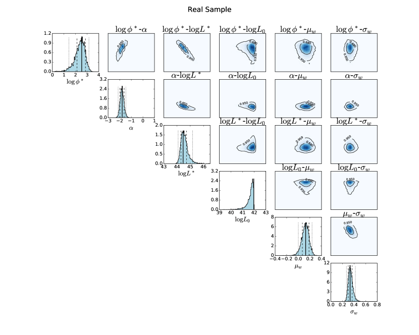
Figure 1: Posterior distributions showing the inferred parameters of the FRB LF. In this “corner plot”, the diagonal histograms are the marginalised one-dimensional posterior distributions for all the parameters. For the parameters except $\log L_{0}$, the solid lines denote the most probable measured values, the dashed lines and dotted lines denote 68% and 95% confidence interval, respectively. For $\log L_{0}$, due to the limited sample size, we do not measure the value and the solid line represents the upper limit value with 95% confidence level (C.L.). The off-diagonal contour plots are for the marginalised two-dimensional posteriors, where the parameter pairs are indicated in the plot titles. The inner and outer black contours are for 68% and 95% confidence intervals, respectively.

The measured LF parameters within 95% confidence interval are $\phi^{*}=339_{-313}^{+1074}\,\mathrm{Gpc}^{-3}\,\mathrm{yr}^{-1}$, $\alpha=-1.79_{-0.35}^{+0.31}$ and $\log L^{*}=44.46_{-0.38}^{+0.71}$. We can not measure the value of the lower cut-off luminosity, due to the limited size of FRB sample. Its upper limit is $\log L_{0}\leq 41.96$. The mean value of pulse width distribution is $\mu_{w}=0.13_{-0.13}^{+0.11}$ and the standard deviation of it is $\sigma_{w}=0.33_{-0.06}^{+0.09}$. We also use the posterior to compute the confidence region of FRB LF, where the 2-$\sigma$ region is shown in Figure 2a.

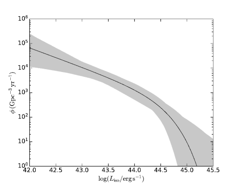
(a) The FRB LF

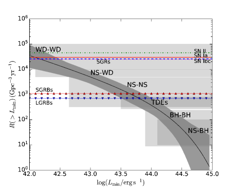
(b) The cumulative event rate density of FRBs

Figure 2: (a) The x-axis is logarithmic luminosity, the y-axis is the luminosity function defined as event rate per unit co-moving volume per logarithmic luminosity. The black solid curve represents the most probable LF shape with the gray shade indicating 2-$\sigma$ confidence region. (b) The x-axis is the threshold luminosity in logarithmic form, the y-axis is cumulative event rate density above the threshold luminosity. The black solid curve with grey shaded region represents the volumetric event rate of FRB population in 2-$\sigma$ C.L. The merger rate of WD-WD, NS-WD, NS-NS, BH-BH, NS-BH and the TDE rate are marked with six shaded regions. Meanwhile, we also plot the volumetric rate of such transients with six lines, i.e., SN Ia (red solid line), Ibc (blue dashed line), II (green dash-dotted line), SGRs (magenta dotted line), SGRBs (red solid line with up-pointing triangles) and LGRBs (blue solid line with down-pointing triangles).

To characterize the event rate distribution of the whole FRB population, we integrate the LF (Equation (11)) from a minimum luminosity $L_{\rm min}$ to infinity as follows:

$$R_{\rm FRB}(>L_{\rm min})=\int_{L_{\rm min}/L^{*}}^{\infty}\phi^{*}\left(\frac{L}{L^{*}}\right)^{\alpha}\,\mathrm{d}\left(\frac{L}{L^{*}}\right)=\phi^{*}\Gamma\left(\alpha+1,\frac{L_{\rm min}}{L^{*}}\right)\,,$$ (26)

where $\Gamma$ is the incomplete Gamma function. The cumulative event rate distribution as a function of $L_{\rm min}$ is shown in Figure 2b.

Similar to L18, we can also estimate the luminosity of individual FRB without marginalisation. The broad luminosity range of all the published FRB sample can be visualised clearly on the Flux-$\mathrm{DM}_{\rm E}$ diagram (Figure 3), which is consistent with results of Shannon et al. (2018). In particular, there appears to be a boundary between repeating (e.g. FRB 121102 (Spitler et al., 2016), FRB 171019 (Kumar et al., 2019) and CHIME repeaters (CHIME/FRB Collaboration et al., 2019b, c; Fonseca et al., 2020)) and non-repeating FRBs around luminosity $10^{42}-10^{43}\,\mathrm{erg}\,\mathrm{s}^{-1}$.

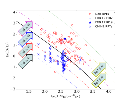
Figure 3: Flux-$\mathrm{DM}_{\rm E}$ diagram. The flux density of each FRB is adopted from FRBCAT or corresponding literature, $\mathrm{DM}_{\rm E}$ is obtained after removing the Galactic DM using the NE2001 electron model (Cordes & Lazio, 2002) We plot all the FRBs published by January 2020, including repeaters (RPTs) and non-repeaters (Non-RPTs). The red hollow dots denote non-repeating FRBs, while repeating FRBs are labelled with blue markers, i.e. FRB 121102 (plus), FRB 171019 (star) and CHIME repeaters (cross). The six curves that run diagonally are the maximum luminosities assuming that all $\mathrm{DM}_{\rm E}$ comes from cosmological contribution without host galaxy or local contribution. For each curve, the corresponding arrow indicates the luminosity values.

3.2 Detection rate

Using the LF, we can study the apparent detection rate (i.e., the number of detections expected per day) for a given telescope. The detection rate is computed from

$$\lambda(\Omega,S_{\rm min}) =\frac{\mathrm{d}N_{\mathrm{obs}}(>S_{\rm min})}{\mathrm{d}t_{\mathrm{obs}}}$$ (27)

$$=\int_{0}^{\Omega}\mathrm{d}\Omega\int_{0}^{\infty}\frac{1}{1+z}\frac{r(z)^{2}}{H(z)}\,\mathrm{d}z\int f_{\mathrm{w}}(\log w_{\mathrm{i}})\,\mathrm{d}\log w_{\mathrm{i}}$$

$$\quad\cdot\int_{\log L_{\mathrm{min}}(w_{\mathrm{o}})}^{\infty}I(\log L)\,\mathrm{d}\log L\,.$$

The results are shown in Figure 4, where eleven telescopes performing FRB searches are also indicated.

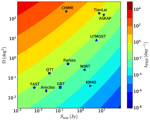
Figure 4: The FRB detection rate map. The x-axis is the detection threshold in flux, the y-axis is the field of view, the color bar on the right indicates the apparent detection rate, i.e., expected detection number of FRBs per day. Eleven telescopes are marked in the map. The fields of view and sensitivities come from corresponding references: Parkes (Staveley-Smith et al., 1996), Arecibo (Spitler et al., 2014), GBT (Masui et al., 2015), UTMOST (Caleb et al., 2017), ASKAP (Shannon et al., 2018), CHIME (CHIME/FRB Collaboration et al., 2018), TianLai (Chen, 2012), FAST(Nan et al., 2011), QTT(Wang, 2017), NSRT and KM40 (Men et al., 2019). The extension of FoV using multibeam or phase array are considered if available at the site. The signal to noise threshold of valid FRB detections is set as 10 for all of telescopes plotted here.

For single-dish telescopes without multibeam or phased array feeds, the telescope diameter determines both field of view and sensitivity. Thus, for a given bandwidth, system temperature, and detection threshold, the detection rate is determined only by the diameter of telescope and LF. As shown in Figure 5, there is an optimal diameter for the telescope to maximize the detection rate.

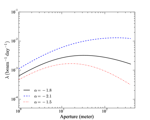
Figure 5: The relation between FRB detection rate and telescope diameter. In this analysis we have assumed a telescope central frequency of 1.4 GHz, bandwidth 300 MHz, $T_{\rm sys}=25\,{\rm K}$. The detection rate depends on the shape of luminosity function, where three curves with power-law indices of $-1.5$, $-1.8$ and $-2.1$ are plotted, which correspond to our 2-$\sigma$ confidence region of the luminosity power-law index. For the most-likely $\alpha$ value, the optimal telescope diameter is about 30 m.

Using the detection rate in Equation (27), we compare the expected detection number with the real detection number of these surveys we used (see Table 3). These two sets of numbers are consistent within 2-$\sigma$ confidence.

Table 3: Detection numbers check for the FRB surveys used in this work.

Survey	PKS-MC	HTRU&SUPERB	PALFA	GBTIM	UTMOST-SS	CRAFT
$N_{\rm theo}$a	$1.2_{-1.1}^{+3.9}$	$14.1_{-13.0}^{+45.2}$	$1.2_{-1.1}^{+3.9}$	$0.33_{-0.30}^{+1.05}$	$5.8_{-5.4}^{+18.7}$	$28.7_{-26.4}^{+92.0}$
$N_{\rm real}$b	2	19	1	1	3	20

• (a) Theoretical detection number with 2-$\sigma$ errors

• (b) The actual detection number as observed in FRB surveys.

4 Discussion and conclusions

4.1 The measurements

Our measurements of the power-law index and the upper cut-off luminosity are $\alpha=-1.79_{-0.35}^{+0.31}$ and $\log L^{*}=44.46_{-0.38}^{+0.71}$, respectively. For both of the parameters, the values match the previous results of L18, who used less number of FRB and obtained $\alpha=-1.57_{-0.37}^{+0.40}$ and $\log L^{*}=44.31_{-0.27}^{+0.22}$. The new FRBs from ASKAP sample are brighter, and slightly increases the cut-off luminosity. We still have not yet measured the intrinsic lower limit of luminosity ($L_{0}$), due to the missing of sufficient low-luminosity FRBs in the current sample. In the future, such FRBs found by larger telescopes should help us to understand and constrain the LF shape and extent at the low-luminosity end.

Our inferred event rate density (also called volumetric event rate) agrees with the previous estimations. Cao et al. (2018) and Deng et al. (2019) derived the FRB volumetric event rate as $R_{\rm FRB}=(3-6)\times 10^{4}\,\mathrm{Gpc}^{-3}\,\mathrm{yr}^{-1}$ and $R_{\rm FRB}=1.8\pm 0.3\times 10^{4}\,\mathrm{Gpc}^{-3}\,\mathrm{yr}^{-1}$, respectively, using the FRB samples containing 22 and 28 Parkes FRBs. Although we have not obtained the intrinsic lower limit of the LF, once we integrate the LF above luminosity of $10^{42}\,\mathrm{erg}\,\mathrm{s}^{-1}$, we can calculate that $R_{\rm FRB}=3.5_{-2.4}^{+5.7}\times 10^{4}\,\mathrm{Gpc}^{-3}\,\mathrm{yr}^{-1}$. This is consistent with the estimations made by the two previous works. For the other threshold luminosities, such as $10^{43}$ and $10^{44}\,\mathrm{erg}\,\mathrm{s}^{-1}$, our measurements give the event rate densities as $5.0_{-2.3}^{+3.2}\times 10^{3}$ and $3.7_{-2.0}^{+3.5}\times 10^{2}\,\mathrm{Gpc}^{-3}\,\mathrm{yr}^{-1}$, respectively. In particular, our measured volumetric rate distribution is identical with the energy function derived by Lu & Piro (2019) from $10^{31}$ to $10^{32}\,\rm erg\,Hz^{-1}$ based on 20 ASKAP FRBs.

Our work focuses on the LF of the sample that mainly consists of non-repeating FRBs. This is very different from work by James (2019), who derived an upper-limit on the repeating FRB density of $\leq 27\,{\rm Gpc}^{-3}$ assuming certain repeating rate and pulse energy distribution. Although it is not legitimate to compare the densities of repeating FRBs with the LF in the current paper, the much higher FRB source density in our paper also indicates that the FRB 121102 is not a typical FRB source as already discussed by James (2019), see also Palaniswamy et al. (2018); Caleb et al. (2019); Li et al. (2019). Either its burst rate is higher than the majority of FRBs or its burst events are highly correlated in time.

We include no spectral modelling in the current paper and have assumed that the FRB spectrum is flat around 1.4 GHz. This is a limitation inherited from the current FRB sample, where most of FRBs used in our computation were detected at $\sim 1.4\,\rm GHz$. The limited frequency coverage also prevents us from detailed modelling of the spectrum. We postpone the spectrum modelling to future work, when a wider frequency coverage is available. The flat-spectrum assumption is driven by the repeater FRB 121102, for which an apparently flat spectrum with $\sim 1\,\rm GHz$ bandwidth was observed (Gajjar et al., 2018).

We have neglected the scattering effects. The reasons for this are twofold: 1) The FRBs used in the current paper is not scattering limited, i.e., there is no indication that scattering downgrade the S/N by order of magnitude; 2) The uncertainty of our LF is still rather large (more than a factor of 10). Our error mainly comes from the limited FRB sample size and the uncertainty of FRB distance. The caveat is that the event rate of distant FRBs seen by large telescopes (e.g., FAST) may be overestimated, since these FRBs might be scattering limited.

4.2 Constraints on the possible origins

The origins of FRBs are still highly debating and many models have been proposed to explain the phenomena (e.g. Platts et al., 2019). The models invoke young pulsars (Cordes & Wasserman, 2016; Connor et al., 2016a), relatively old magnetars as observed (Popov & Postnov, 2010; Katz, 2016), putative young magnetars born from gamma-ray bursts and superluminous supernovae (SNe) (Murase et al., 2016; Metzger et al., 2017; Wang et al., 2018), normal pulsars with external interactions (Zhang, 2017), among others. The catastrophic (non-repeating) models include various types of compact star mergers, such as white dwarf (WD) - WD mergers (Kashiyama et al., 2013), neutron star (NS) - NS mergers (Totani, 2013; Wang et al., 2016), NS - black hole (BH) mergers (Zhang, 2019; Dai, 2019), and even BH - BH mergers (Zhang, 2016; Liu et al., 2016), or collapses of supramassive neutron stars into black holes (Falcke & Rezzolla, 2014; Zhang, 2014). The expected event rates of these scenarios differ, and by comparing with our results, one can constrain the models.

In Figure 2b, we list a few types of burst-like events that are possibly associated with FRBs, including: 1) stellar BH-BH mergers, $R_{\rm BH-BH}=(9-240)\,\mathrm{Gpc}^{-3}\,\mathrm{yr}^{-1}$ (Abbott et al., 2016); 2) NS-NS mergers, $R_{\rm NS-NS}=1.5_{-1.2}^{+3.2}\times 10^{3}\,\mathrm{Gpc}^{-3}\,\mathrm{yr}^{-1}$ (Abbott et al., 2017); 3) NS-BH mergers, $R_{\rm NS-BH}=(10-100)\,\mathrm{Gpc}^{-3}\,\mathrm{yr}^{-1}$ (Mapelli & Giacobbo, 2018); 4) NS-WD mergers, $R_{\rm NS-WD}=(0.5-1)\times 10^{4}\,\mathrm{Gpc}^{-3}\,\mathrm{yr}^{-1}$ (Thompson et al., 2009); 5) WD-WD mergers, $R_{\rm WD-WD}=(10^{4}-10^{5})\,\mathrm{Gpc}^{-3}\,\mathrm{yr}^{-1}$ (Badenes & Maoz, 2012); 6) tidal disruption events (TDEs), $R_{\rm TDEs}=4.8_{-2.1}^{+3.2}\times 10^{2}\,\mathrm{Gpc}^{-3}\,\mathrm{yr}^{-1}$ (Sun et al., 2015); 7) three types of supernovae (SNe), i.e., SN Ia ($R_{\rm SNIa}=3\times 10^{4}\,\mathrm{Gpc}^{-3}\,\mathrm{yr}^{-1}$), Ibc ($R_{\rm SNIbc}=2.5\times 10^{4}\,\mathrm{Gpc}^{-3}\,\mathrm{yr}^{-1}$) and II ($R_{\rm SNII}=4.5\times 10^{4}\,\mathrm{Gpc}^{-3}\,\mathrm{yr}^{-1}$) (Li et al., 2011b); 8) soft gamma-ray repeaters (SGRs), $R_{\rm SGRs}<2.5\times 10^{4}\,\mathrm{Gpc}^{-3}\,\mathrm{yr}^{-1}$ (Ofek, 2007; Kulkarni et al., 2014); 9) short gamma-ray bursts (SGRBs, beaming-corrected rate), $R_{\rm SGRBs}=1.1\times 10^{3}\,\mathrm{Gpc}^{-3}\,\mathrm{yr}^{-1}$ (Coward et al., 2012; Sun et al., 2015); 10) long gamma-ray bursts (LGRBs), $R_{\rm LGRBs}=7\times 10^{2}\,\mathrm{Gpc}^{-3}\,\mathrm{yr}^{-1}$ (Chapman et al., 2007; Sun et al., 2015). The event rate densities of the transients above and the associated FRB threshold luminosities are summarized in Table 4.

Table 4: The possibly associated transients

Transient	$R\,(\mathrm{Gpc}^{-3}\,\mathrm{yr}^{-1})$a	$\log(L_{\mathrm{min}}/\mathrm{erg}\,\mathrm{s}^{-1})$b	Ref.c
BH-BH	$(9-240)$	$(44.1-44.7)$	[1]
NS-NS	$1.5_{-1.2}^{+3.2}\times 10^{3}$	$43.5\pm 0.5$	[2]
NS-BH	$(10-100)$	$(44.3-44.7)$	[3]
NS-WD	$(0.5-1)\times 10^{4}$	$(42.7-43.0)$	[4]
WD-WD	$(10^{4}-10^{5})$	$(41.4-42.7)$	[5]
TDEs	$4.8_{-2.1}^{+3.2}\times 10^{2}$	$43.9\pm 0.2$	[6]
SN Ia	$3\times 10^{4}$	$42.1$	[7]
SN Ibc	$2.5\times 10^{4}$	$42.2$	[7]
SN II	$4.5\times 10^{4}$	$41.9$	[7]
SGRs	$<2.5\times 10^{4}$	$>42.2$	[8][9]
SGRBs	$1.1\times 10^{3}$	$43.6$	[6][10]
LGRBs	$7\times 10^{2}$	$43.8$	[6][11]

• (a) Event rate density in units of $\mathrm{Gpc}^{-3}\,\mathrm{yr}^{-1}$.

• (b) The threshold luminosity in FRB LF for the associated transient.

• (c) The references are: [1] Abbott et al. (2016); [2] Abbott et al. (2017); [3] Mapelli & Giacobbo (2018); [4] Thompson et al. (2009); [5] Badenes & Maoz (2012); [6] Sun et al. (2015); [7] Li et al. (2011a); [8] Ofek (2007) [9] Kulkarni et al. (2014); [10] Coward et al. (2012); [10] Chapman et al. (2007).

An immediate inference from Figure 2b is that the FRB event rate density above $10^{42}\,\mathrm{erg}\,\mathrm{s}^{-1}$ is comparable to that of supernovae, as known before (Thornton et al., 2013), but is greater than most compact star merger models. The WD-WD merger rate density is viable and is consistent with the Type Ia SN rate density. However, no SN has been observed to be associated with any FRB event, suggesting that a direct connection between FRBs and SN explosions can be ruled out. One may consider the scenarios that invoke once-in-a-life-time events from isolated neutron stars born from SN explosions, which may interpret the FRB event rate density. However, such genuinely non-repeating models proposed so far only apply to a sub-categories of SNe. For example, the “blitzar” model involving collapses of supramassive NSs to BHs (Falcke & Rezzolla, 2014) only applies to those SN explosions that form rapidly spinning, massive NSs whose gravitational mass exceeds the maximum mass of a non-spinning NS, which only comprise a small fraction of all SNe. Such a model may only account to a small fraction of FRBs (e.g. in the high-luminosity end). Another scenario invoking the product of SN explosions is the young magnetar model (Murase et al., 2016; Metzger et al., 2017; Wang et al., 2018). This model also requires a special type of the progenitor system (e.g. those producing long GRBs or superluminous supernovae), and hence, is also only relevant for a small fraction of SN explosions. On the other hand, compared with the blitzar model, the young magnetar model can produce multiple bursts in its life time, making it possible to account for the majority of FRBs if most (if not all) of them are repeating sources (e.g. Ravi, 2019).

Our results show that it is unlikely that all FRBs come from BH-BH, BH-NS or NS-NS mergers, if each merger event generates only one FRB. If such system can produce multiple FRBs, a substantial number of FRBs would be generated from each merger. The required multiplicity number of FRBs from each merger would be $10^{2}-10^{4}$ for BH-BH mergers, $10-100$ for NS-NS mergers, and $100-1000$ for NS-BH mergers. It can be difficult to produce many bursts associating with the merger event over the period of several years (as observed in FRB 121102). One possible scenario would be to invoke an NS-NS post-merger stable magnetar that can survive the merger (e.g. Zhang & Mészáros, 2001; Metzger et al., 2008; Bucciantini et al., 2012; Rezzolla & Kumar, 2015; Margalit et al., 2019; Wang et al., 2020). However, this requires a stiff NS equation of state and small masses in the NS-NS merger systems. Another possibility is that repeating FRBs are produced decades to centuries before the merger when the magnetospheres of the two NSs interact relentlessly (Zhang, 2020).

On the other hand, our results do not object the possibility that a small fraction of FRBs, probably on the high-luminosity end, may be related to compact star mergers. Figure 2b shows that for $L>10^{43}\,\mathrm{erg}\,\mathrm{s}^{-1}$, the merger models become viable. For example, an NS-NS merger may produce a bright FRB during the merger phase, which can be followed by weaker repeating bursts from a post-merger NS (Jiang et al., 2019).

It is interesting to note that the observed non-repeating FRBs typically have high luminosities with $L>10^{43}\,\mathrm{erg}\,\mathrm{s}^{-1}$, whereas the luminosity of the repeating bursts is usually smaller. This could account for the absence of repeaters detected by Parkes (Petroff et al., 2015b) and ASKAP (James, 2019) due to the sensitivity limits of the telescopes. One may suspect that the low-luminosity FRBs ($L<10^{43}\,\mathrm{erg}\,\mathrm{s}^{-1}$) could potentially be the repeater candidates, because of their higher event rate and the existence of a plausible border in Figure 3. With the same method in L18, we calculate the luminosity for individual FRB and predict a list of repeater candidates in the current FRBCAT, as shown in Table 5.

Table 5: The repeating FRB candidates according to the plausible luminosity clustering

FRB	$\log(L_{\mathrm{iso}}/\mathrm{erg}\,\mathrm{s}^{-1})$a	Telescope	Ref.b
010621	$41.8^{+0.3}_{-0.7}$	Parkes	[1][2]
120127	$42.9^{+0.3}_{-0.6}$	Parkes	[3]
140514	$42.9^{+0.3}_{-0.6}$	Parkes	[4]
141113	$40.7^{+0.3}_{-0.6}$	Arecibo	[5]
171020	$42.5^{+0.3}_{-0.9}$	ASKAP	[6]
180301	$42.4^{+0.4}_{-0.6}$	Parkes	[7]
180729.J1316+55	$42.9^{+0.5}_{-0.8}$	CHIME	[8]
180923	$42.3^{+0.3}_{-0.6}$	Parkes	[9]

• (a) The inferred isotropic luminosity within 95% confidence interval.

• (b) The references are: [1] Keane et al. (2011); [2] Keane et al. (2012); [3] Thornton et al. (2013); [4] Petroff et al. (2015a); [5] Patel et al. (2018); [6] Shannon et al. (2018); [7] Price et al. (2019); [8] CHIME/FRB Collaboration et al. (2019a); [9] Bhandari et al. (2018b).

4.3 Searching plan

The FRB detection rate as a function of minimum detection flux and field of view is given in Figure 4. Obviously, telescopes with high gain and large field of view are the best for FRB searching, e.g.m CHIME and TianLai (CHIME/FRB Collaboration et al., 2018; Chen, 2012). Thanks to 13 beams receiver (Staveley-Smith et al., 1996), the Parkes 64-m radio telescope has played a pioneering role in FRB searching ever since its serendipitous discovery of the “Lorimer Burst” (Lorimer et al., 2007). Meanwhile, equipped with a 19-beam receiver (Li et al., 2018), FAST can achieve a detection rate at the same level with Parkes telescope (see Figure 4, about $5\times 10^{-2}\,\mathrm{day}^{-1}$). This provides excellent prospects to detect many high-DM FRBs ($>3000\,\mathrm{cm}^{-3}\,\mathrm{pc}$), see also Zhang (2018). Nevertheless, since the scattering effects is not included in the computation, the high gain telescopes (e.g., Arecibo and FAST) may detect less FRBs, if FRBs are in the scattering-limited regime.

For single-beam system, we calculated the detection rate - diameter relation as shown in Figure 5. For the central value of LF, the optimal diameter of single-beam telescopes to detect FRBs is 30–40 m. Future discoveries made by CHIME, FAST, ASKAP and other instruments are probably crucial to our understanding for the FRB population. We anticipate that the methodologies developed in this paper and in L18 will form an important component in the analysis of these findings.

Appendix A Derivation of marginalised likelihood

More detailed calculation can be found in L18, here we just outline the major steps constructing the likelihood.

The relations of isotropic luminosity - flux, intrinsic width - observed width and dispersion measures are

$$\log L = \log S+2\log d_{\rm L}+\log\Delta\nu_{0}-\log\epsilon+\log 4\pi\,,$$ (28)

$$w_{\mathrm{i}} = \frac{w_{\mathrm{o}}}{1+z}\,,$$ (29)

$$\mathrm{DM}_{\rm host} = (\mathrm{DM}_{\rm E}-\mathrm{DM}_{\rm IGM})(1+z)-\mathrm{DM}_{\rm src}\,,$$ (30)

where $d_{\rm L}$ is the luminosity distance, $\Delta\nu_{0}$ is the spectrum width. Note that in this paper, we use a flat spectrum as the FRB spectrum and fix the spectrum width at a reference value $\Delta\nu_{0}=1\,\rm GHz$. $\mathrm{DM}_{\rm IGM}$ is the DM contributed by intergalactic medium (IGM), given by (Deng & Zhang, 2014)

$$\mathrm{DM}_{\rm IGM}(z)=\frac{\rho_{\rm c}\Omega_{\rm b}f_{\rm IGM}}{m_{\rm p}H_{0}}\int\frac{g(z)(1+z)}{E(z)}\,\mathrm{d}z\,,$$ (31)

where $m_{\rm p}$ is the proton mass, $H_{0}$ is the Hubble constant. $\rho_{c}$ is the current critical density of the universe, $\Omega_{b}$ is the mass fraction in the universe. The $f_{\mathrm{IGM}}$ is the cosmological baryon mass fraction in the IGM, here we use $f_{\mathrm{IGM}}\simeq 0.83$ (Fukugita et al., 1998). The function $g(z)$ is the ionized electron number fraction per baryon, given as

$$g(z)\simeq\frac{3}{4}\chi_{e,\mathrm{H}}(z)+\frac{1}{8}\chi_{e,\mathrm{He}}(z)\,,$$ (32)

where $\chi_{e,\mathrm{H}}$ and $\chi_{e,\mathrm{He}}$ are the cosmic ionization fraction of hydrogen and helium, respectively.

Based on Equation (28), (29) and (30), we can convert the PDF $f(\log L,\log w_{\mathrm{i}},N,z,\mathrm{DM}_{\rm host},\mathrm{DM}_{\rm src},\log\epsilon)$ to $f(\log S,\log w_{\mathrm{o}},N,\mathrm{DM}_{\rm E},z,\mathrm{DM}_{\rm src},\log\epsilon)$ using the Jacobian transformation, i.e.

$$f(\log S,\log w_{\mathrm{o}},N,\mathrm{DM}_{\rm E},z,\mathrm{DM}_{\rm src},\log\epsilon)$$ (33)

$$={} |{\mathbf{{J}}}|\,f(\log L,\log w_{\mathrm{i}},N,\mathrm{DM}_{\rm host},z,\mathrm{DM}_{\rm src},\log\epsilon)\,,$$

where the Jacobian determinant is written as

$$\begin{split}\left|{\mathbf{{J}}}\right|&=\left|\frac{\partial(\log L,\,\log w_{\mathrm{i}},\,N,\,\mathrm{DM}_{\rm host},\,z,\,\mathrm{DM}_{\rm src},\,\log\epsilon)}{\partial(\log S,\,\log w_{\mathrm{o}},\,N,\,\mathrm{DM}_{\rm E},\,z,\,\mathrm{DM}_{\rm src},\,\log\epsilon)}\right|\\ &=\left|\begin{pmatrix}1&0&0&0&\partial\log L/\partial z&0&-1\\ 0&1&0&0&w_{\mathrm{o}}/(\ln 10\,w_{\mathrm{i}}(1+z)^{2})&0&0\\ 0&0&1&0&0&0&0\\ 0&0&0&1+z&\partial\mathrm{DM}_{\rm host}/\partial z&-1&0\\ 0&0&0&0&1&0&0\\ 0&0&0&0&0&1&0\\ 0&0&0&0&0&0&1\\ \end{pmatrix}\right|\\ &=1+z.\end{split}$$

One gets

$$f(\log S,\log w_{\mathrm{o}},N,\mathrm{DM}_{\rm E},z,\mathrm{DM}_{\rm src},\log\epsilon)$$ (34)

$$={}\phi(\log L)\,f_{\mathrm{w}}(\log w_{\mathrm{i}})\,P(N)\,f_{\cal D}(\mathrm{DM}_{\rm host}|z)\,f_{z}(z)\,f_{\mathrm{s}}(\mathrm{DM}_{\rm src})$$

$$\quad\cdot f_{\mathrm{\epsilon}}(\log\epsilon)\,(1+z)\,,$$

Adding the likelihood for the number of events to above equation, we have

$$f(\log S,\log w_{\mathrm{o}},N,\mathrm{DM}_{\rm E},z,\mathrm{DM}_{\rm src},\log\epsilon)$$ (35)

$$={}P(N)\cdot f(\log S,\log w_{\mathrm{o}},\mathrm{DM}_{\rm E},z,\mathrm{DM}_{\rm src},\log\epsilon)\,,$$

We marginalise the $f(\log S,\log w_{\mathrm{o}},\mathrm{DM}_{\rm E},z,\mathrm{DM}_{\rm src},\log\epsilon)$ by integrating $z,\mathrm{DM}_{\rm src}$ and $\log\epsilon$.

$$f(\log S,\log w_{\mathrm{o}},\mathrm{DM}_{\rm E}) =\frac{1}{N_{\mathrm{f}}}\int_{0}^{\infty}I(\log L)\,f_{\mathrm{w}}(\log w_{\mathrm{i}})f_{z}(z)\,$$ (36)

$$\quad I(\mathrm{DM}_{\rm E},z)\,(1+z)\,\mathrm{d}z,$$

The marginalisation of $\mathrm{DM}_{\rm src}$ leads to

$$I(\mathrm{DM}_{\rm E},z) =\int_{0}^{\max(\mathrm{DM}_{\rm src})}f_{\cal D}(\mathrm{DM}_{\rm host}|z)f_{\mathrm{s}}(\mathrm{DM}_{\rm src})\,\mathrm{d}\mathrm{DM}_{\rm src}\,,$$ (37)

and the marginalisation of $\log\epsilon$ gives

$$I(\log L)=\int\phi(\log L)f_{\mathrm{\epsilon}}(\log\epsilon)\,\mathrm{d}\log\epsilon.$$ (38)

The normalisation factor for $f(\log S,\log w_{\mathrm{o}},\mathrm{DM}_{\rm E},z)$ becomes

$$N_{\mathrm{f}} =\int_{\log S_{\rm min}(w_{\mathrm{o}})}^{\infty}\,\mathrm{d}\log S\int\int\int f(\log S,\log w_{\mathrm{o}},\mathrm{DM}_{\rm E},z)\,$$ (39)

$$\quad\cdot\mathrm{d}\log w_{\mathrm{o}}\,\mathrm{d}\mathrm{DM}_{\rm E}\,\mathrm{d}z.$$

The lower limit of the flux density integration, $S_{\rm min}$, is the minimum detectable flux density for the telescope at the time when a given FRB with pulse width $w_{\mathrm{o}}$ was detected, which is mentioned in Equation (10) in the main text.

The final marginalised likelihood function is

$$\mathcal{L}=\mathcal{L}(N)\cdot\mathcal{L}(\log S,\log w_{\mathrm{o}},\mathrm{DM}_{\rm E})\,,$$ (40)

where

$$\mathcal{L}(\log S,\log w_{\mathrm{o}},\mathrm{DM}_{\rm E}) =\frac{1}{N_{\mathrm{f}}}\int_{0}^{\infty}I(\log L)\,f_{\mathrm{w}}(\log w_{\mathrm{i}})\,f_{z}(z)\,$$ (41)

$$\quad\cdot I(\mathrm{DM}_{\rm E},z)\,(1+z)\,\mathrm{d}z,$$

and

$$\mathcal{L}(N)=\frac{(\rho\Omega t)^{N}e^{-\rho\Omega t}}{N!}\,.$$ (42)

Compared to the method of L18, we add the modelling for the number of events, which is the key to the even rate density inference.

Appendix B Derivation on the surface event rate of survey

For the $k$-th FRB in the $j$-th survey, the surface event rate is defined as the partial derivative of detection number $N$ to observing time $t_{\rm obs}$ and FoV $\Omega$,

$$\rho_{kj} =\frac{\partial N(>S_{\mathrm{min},\,kj})}{\partial t_{\mathrm{obs}}\partial\Omega}$$ (43)

$$=\int\frac{\partial V}{\partial\Omega\partial z}\mathrm{d}z\int_{L_{\mathrm{min},\,kj}}^{\infty}\frac{\partial N}{\partial V\partial t_{\mathrm{obs}}\,\partial\log L}\mathrm{d}\log L$$

$$=\int\frac{\mathrm{d}t}{\mathrm{d}t_{\mathrm{obs}}}\frac{\partial V}{\partial\Omega\partial z}\mathrm{d}z\int_{L_{\mathrm{min},\,kj}}^{\infty}\mathrm{d}\log L\,\int_{\log\frac{1}{2}}^{0}\frac{\partial N}{\partial V\,\partial t\,\partial\log L\,\partial\log\epsilon}$$

$$\quad\cdot\mathrm{d}\log\epsilon\,$$

$$=\int_{0}^{\infty}\frac{1}{1+z}\frac{r(z)^{2}}{H(z)}\mathrm{d}z\int_{\log L_{\mathrm{min}},\,kj}^{\infty}I(\log L)\,\mathrm{d}\log L\,.$$

The lower limit of above luminosity integral is determined by $L_{\mathrm{min},\,kj}=\max(L_{0},L_{\mathrm{thre},\,kj})$, where $L_{0}$ is the intrinsic lower cut-off of LF and threshold luminosity of survey $L_{\mathrm{thre}}$ is given as

$$L_{\mathrm{thre},\,kj}\equiv 4\pi d_{\rm L}^{2}\Delta\nu_{0}S_{\mathrm{min},\,kj}\,,$$ (44)

where the flux threshold of FRB with a duration $w_{\mathrm{o},\,kj}$ is

$$S_{\mathrm{min},kj}=\frac{\mathrm{S/N}_{0}\ T_{\mathrm{sys}}}{G\sqrt{N_{\mathrm{p}}\,\mathrm{BW}\,w_{\mathrm{o},\,kj}}}\,.$$ (45)

Alternatively, if we marginalise the luminosity in advance, the surface event rate in Equation (43) would be re-written as

$$\rho_{kj} =\int_{0}^{\infty}\frac{1}{1+z}\frac{r(z)^{2}}{H(z)}\mathrm{d}z\,\int_{\log\frac{1}{2}}^{0}\phi^{*}\Gamma\left(\alpha+1,\frac{L_{\mathrm{min},\,kj}}{\epsilon L^{*}}\right)f_{\mathrm{\epsilon}}(\log\epsilon)$$ (46)

$$\quad\cdot\mathrm{d}\log\epsilon\,,$$

where $\Gamma$ is the incomplete gamma function. Due to the FRB width distribution $f_{\mathrm{w}}(\log w_{\mathrm{o}})$, the total FRB surface rate becomes

$$\rho_{j}=\int\rho(w_{\mathrm{o}})\,f_{\mathrm{w}}(\log w_{\mathrm{o}})\,\mathrm{d}\log w_{\mathrm{o}}\,.$$ (47)

Overall, one will have the surface rate of $j$-th survey by marginalising the FRB intrinsic widths,

$$\rho_{j} =\int_{0}^{\infty}\frac{1}{1+z}\frac{r(z)^{2}}{H(z)}\mathrm{d}z\int f_{\mathrm{w}}(\log w_{\mathrm{i}})\,\mathrm{d}\log w_{\mathrm{i}}$$ (48)

$$\quad\cdot\int_{\log L_{\mathrm{min}}(w_{\mathrm{o}})}^{\infty}I(\log L)\,\mathrm{d}\log L,$$

where $I(\log L)=\int\phi(\log L)f_{\mathrm{\epsilon}}(\log\epsilon)\,\mathrm{d}\log\epsilon$.

Appendix C Adding independent Poisson processes

Denote $\lambda_{1}$ and $\lambda_{2}$ as the rates of two independent event $X$ and $Y$, respectively. We now compute the event rate of detecting either one of them. If we divide the total observing time $t$ into $n$ pieces, the probability of detecting $k$ events in all $n$ durations is

$$P(X+Y=k) =\binom{n}{k}\sum_{i=0}^{k}\left[\binom{k}{i}(\lambda_{1}\Delta t)^{i}(\lambda_{2}\Delta t)^{k-i}(1-\lambda_{1}\Delta t)^{n-i}\right.$$ (49)

$$\quad\left.\cdot(1-\lambda_{2}\Delta t)^{n-k+i}\right]$$

$$=\binom{n}{k}\sum_{i=0}^{k}\left[\binom{k}{i}\left(\frac{\lambda_{1}t}{n}\right)^{i}\left(\frac{\lambda_{2}t}{n}\right)^{k-i}\left(1-\frac{\lambda_{1}t}{n}\right)^{n-i}\right.$$

$$\quad\left.\cdot\left(1-\frac{\lambda_{2}t}{n}\right)^{n-k+i}\right]$$

Using the relation of

$$\lim_{n\to\infty}\left(1-\frac{\lambda t}{n}\right)^{n}=e^{-\lambda t}\,,$$ (50)

one has

$$\lim_{n\to\infty}P(X+Y=k) =\frac{n!}{(n-k)!k!n^{k}}\sum_{i=0}^{k}\left[\frac{k!}{(k-i)!i!}(\lambda_{1}t)^{i}(\lambda_{2}t)^{k-i}\right.$$ (51)

$$\quad\left.\cdot e^{-\lambda_{1}t}e^{-\lambda_{2}t}\right]$$

$$=\frac{e^{-(\lambda_{1}+\lambda_{2})t}}{k!}\sum_{i=0}^{k}\left[\binom{k}{i}(\lambda_{1}t)^{i}(\lambda_{2}t)^{k-i}\right]$$

$$=\frac{[(\lambda_{1}+\lambda_{2})t]^{k}e^{-(\lambda_{1}+\lambda_{2})t}}{k!}\,.$$

This is the continuous time limit. Thus, the event rate is additive and the distribution for the number of detection follows Poisson distribution, if each event is independent. In a similar fashion, we can show that for $N$ random events {${X_{1},X_{2},\cdots,X_{N}}$}, the total rate of detecting any of them is $\lambda=\lambda_{1}+\lambda_{2}+\cdots+\lambda_{N}$.

Appendix D Algorithm verification using the mock data

For the simulations, the information of the two mock surveys are described in Table 6. After Bayesian inference, the posterior distribution of mock FRBs are shown in Figure 6, and the results of parameter inference are listed in Table 7. As one can see, our algorithm correctly recovered parameter central value used in the simulations with 95% confidence.

Table 6: Systematic information of the mock surveys

Survey	G	$T_{\mathrm{sys}}$	BW	$\Omega$	$N_{\mathrm{p}}$	S/N0	$N_{\mathrm{FRB}}$
	(K/Jy)	(K)	(MHz)	($\mathrm{deg}^{2}$)
S1	0.7	30	300	0.55	2	10	100
S2	0.05	100	300	30	2	10	100

Table 7: The results of Bayesian inference for the mock FRBs

Sample	$t_{\rm svy}$ (hr)		$\phi^{*}\,(\mathrm{Gpc}^{-3}\,\mathrm{yr}^{-1})$		$\alpha$		$\log L^{*}\,(\mathrm{erg}\,\mathrm{s}^{-1})$		$\log L_{0}\,(\mathrm{erg}\,\mathrm{s}^{-1})$		$\mu_{w}$		$\sigma_{w}$
	S1	S2	Fid.(a)	Mea.(b)	Fid.	Mea.	Fid.	Mea.	Fid.	Mea.	Fid.	Mea.	Def.	Mea.
I	$15149$	$5366$	$1\times 10^{3}$	$1148_{-424}^{+894}$	$-1.5$	$-1.48_{-0.10}^{+0.13}$	45.0	$45.00_{-0.17}^{+0.15}$	40.0	$\leq 41.8$	0.4	$0.38_{-0.05}^{+0.05}$	0.3	$0.31_{-0.03}^{+0.03}$
II	$1383$	$647$	$1\times 10^{4}$	$7244_{-2458}^{+6559}$	$-1.5$	$-1.57_{-0.08}^{+0.13}$	45.0	$45.10_{-0.18}^{+0.14}$	40.0	$\leq 40.8$	0.4	$0.39_{-0.05}^{+0.04}$	0.3	$0.31_{-0.03}^{+0.04}$

• (a) Fiducial values when we simulate the mock data.

• (b) All the measurements are given within 2-$\sigma$ error.

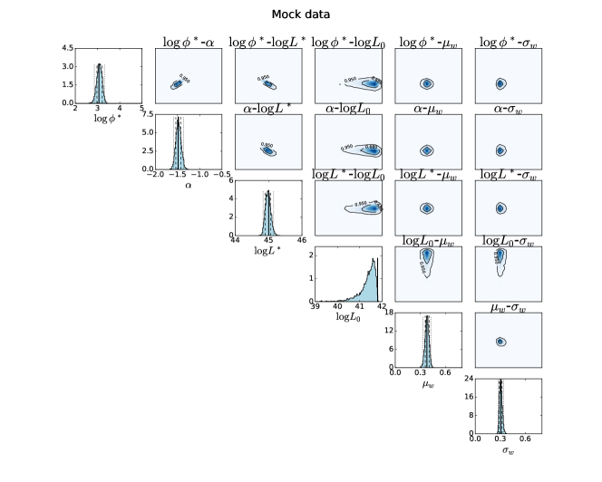
(a) Sample I

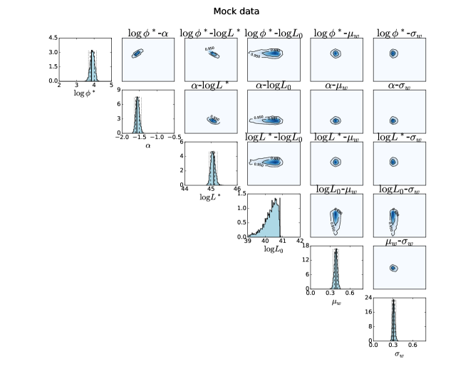
(b) Sample II

Figure 6: Posterior distributions of the inferred parameters of mock FRB samples (I and II). In each panel, subplots are the same as Figure 1.

References

- Abbott et al. (2016) Abbott B. P., et al., 2016, Physical Review X, 6, 041015
- Abbott et al. (2017) Abbott B. P., et al., 2017, Physical Review Letters, 119, 161101
- Badenes & Maoz (2012) Badenes C., Maoz D., 2012, ApJ, 749, L11
- Bannister et al. (2017) Bannister K. W., et al., 2017, ApJ, 841, L12
- Bera et al. (2016) Bera A., Bhattacharyya S., Bharadwaj S., Bhat N. D. R., Chengalur J. N., 2016, MNRAS, 457, 2530
- Bhandari et al. (2018a) Bhandari S., et al., 2018a, MNRAS, 475, 1427
- Bhandari et al. (2018b) Bhandari S., et al., 2018b, The Astronomer’s Telegram, 12060, 1
- Born & Wolf (1999) Born M., Wolf E., eds, 1999, Principles of optics : electromagnetic theory of propagation, interference and diffraction of light. Cambridge University Press, New York
- Bucciantini et al. (2012) Bucciantini N., Metzger B. D., Thompson T. A., Quataert E., 2012, MNRAS, 419, 1537
- CHIME/FRB Collaboration et al. (2018) CHIME/FRB Collaboration et al., 2018, ApJ, 863, 48
- CHIME/FRB Collaboration et al. (2019a) CHIME/FRB Collaboration et al., 2019a, Nature, 566, 230
- CHIME/FRB Collaboration et al. (2019b) CHIME/FRB Collaboration et al., 2019b, Nature, 566, 235
- CHIME/FRB Collaboration et al. (2019c) CHIME/FRB Collaboration et al., 2019c, ApJ, 885, L24
- Caleb et al. (2016) Caleb M., Flynn C., Bailes M., Barr E. D., Hunstead R. W., Keane E. F., Ravi V., van Straten W., 2016, MNRAS, 458, 708
- Caleb et al. (2017) Caleb M., et al., 2017, MNRAS, 468, 3746
- Caleb et al. (2019) Caleb M., Stappers B. W., Rajwade K., Flynn C., 2019, MNRAS, 484, 5500
- Cao et al. (2018) Cao X.-F., Yu Y.-W., Zhou X., 2018, ApJ, 858, 89
- Champion et al. (2016) Champion D. J., et al., 2016, MNRAS, 460, L30
- Chapman et al. (2007) Chapman R., Tanvir N. R., Priddey R. S., Levan A. J., 2007, MNRAS, 382, L21
- Chen (2012) Chen X., 2012, in International Journal of Modern Physics Conference Series. pp 256–263 (arXiv:1212.6278), doi:10.1142/S2010194512006459
- Connor (2019) Connor L., 2019, MNRAS, 487, 5753
- Connor & Petroff (2018) Connor L., Petroff E., 2018, ApJ, 861, L1
- Connor et al. (2016a) Connor L., Sievers J., Pen U.-L., 2016a, MNRAS, 458, L19
- Connor et al. (2016b) Connor L., Pen U.-L., Oppermann N., 2016b, MNRAS, 458, L89
- Connor et al. (2016c) Connor L., Lin H.-H., Masui K., Oppermann N., Pen U.-L., Peterson J. B., Roman A., Sievers J., 2016c, MNRAS, 460, 1054
- Cordes & Lazio (2002) Cordes J. M., Lazio T. J. W., 2002, arXiv e-prints, pp astro–ph/0207156
- Cordes & Wasserman (2016) Cordes J. M., Wasserman I., 2016, MNRAS, 457, 232
- Coward et al. (2012) Coward D. M., et al., 2012, MNRAS, 425, 2668
- Dai (2019) Dai Z. G., 2019, ApJ, 873, L13
- Deng & Zhang (2014) Deng W., Zhang B., 2014, ApJ, 783, L35
- Deng et al. (2019) Deng C.-M., Wei J.-J., Wu X.-F., 2019, Journal of High Energy Astrophysics, 23, 1
- Falcke & Rezzolla (2014) Falcke H., Rezzolla L., 2014, A&A, 562, A137
- Feroz et al. (2009) Feroz F., Hobson M. P., Bridges M., 2009, MNRAS, 398, 1601
- Fonseca et al. (2020) Fonseca E., et al., 2020, ApJ, 891, L6
- Fukugita et al. (1998) Fukugita M., Hogan C. J., Peebles P. J. E., 1998, ApJ, 503, 518
- Gajjar et al. (2018) Gajjar V., et al., 2018, ApJ, 863, 2
- Golpayegani et al. (2019) Golpayegani G., et al., 2019, MNRAS, 489, 4001
- James (2019) James C. W., 2019, MNRAS, 486, 5934
- Jiang et al. (2019) Jiang J., Wang W., Luo R., Du S., Chen X., Lee K., Xu R., 2019, arXiv e-prints, p. arXiv:1909.10961
- Kashiyama et al. (2013) Kashiyama K., Ioka K., Mészáros P., 2013, ApJ, 776, L39
- Katz (2016) Katz J. I., 2016, ApJ, 826, 226
- Keane et al. (2011) Keane E. F., Kramer M., Lyne A. G., Stappers B. W., McLaughlin M. A., 2011, MNRAS, 415, 3065
- Keane et al. (2012) Keane E. F., Stappers B. W., Kramer M., Lyne A. G., 2012, MNRAS, 425, L71
- Keane et al. (2016) Keane E. F., et al., 2016, Nature, 530, 453
- Kulkarni et al. (2014) Kulkarni S. R., Ofek E. O., Neill J. D., Zheng Z., Juric M., 2014, ApJ, 797, 70
- Kumar et al. (2019) Kumar P., et al., 2019, ApJ, 887, L30
- Lawrence et al. (2017) Lawrence E., Vander Wiel S., Law C., Burke Spolaor S., Bower G. C., 2017, AJ, 154, 117
- Li et al. (2011a) Li W., Chornock R., Leaman J., Filippenko A. V., Poznanski D., Wang X., Ganeshalingam M., Mannucci F., 2011a, MNRAS, 412, 1473
- Li et al. (2011b) Li W., et al., 2011b, MNRAS, 412, 1441
- Li et al. (2018) Li D., et al., 2018, IEEE Microwave Magazine, 19, 112
- Li et al. (2019) Li Y., Zhang B., Nagamine K., Shi J., 2019, ApJ, 884, L26
- Liu et al. (2016) Liu T., Romero G. E., Liu M.-L., Li A., 2016, ApJ, 826, 82
- Locatelli et al. (2019) Locatelli N., Ronchi M., Ghirlanda G., Ghisellini G., 2019, A&A, 625, A109
- Lorimer et al. (2007) Lorimer D. R., Bailes M., McLaughlin M. A., Narkevic D. J., Crawford F., 2007, Science, 318, 777
- Lu & Piro (2019) Lu W., Piro A. L., 2019, ApJ, 883, 40
- Luo et al. (2018) Luo R., Lee K., Lorimer D. R., Zhang B., 2018, MNRAS, 481, 2320
- Macquart & Ekers (2018) Macquart J. P., Ekers R. D., 2018, MNRAS, 474, 1900
- Mapelli & Giacobbo (2018) Mapelli M., Giacobbo N., 2018, MNRAS, 479, 4391
- Margalit et al. (2019) Margalit B., Berger E., Metzger B. D., 2019, ApJ, 886, 110
- Masui et al. (2015) Masui K., et al., 2015, Nature, 528, 523
- Men et al. (2019) Men Y. P., et al., 2019, MNRAS, 488, 3957
- Metzger et al. (2008) Metzger B. D., Quataert E., Thompson T. A., 2008, MNRAS, 385, 1455
- Metzger et al. (2017) Metzger B. D., Berger E., Margalit B., 2017, ApJ, 841, 14
- Murase et al. (2016) Murase K., Kashiyama K., Mészáros P., 2016, MNRAS, 461, 1498
- Nan et al. (2011) Nan R., et al., 2011, International Journal of Modern Physics D, 20, 989
- Ofek (2007) Ofek E. O., 2007, ApJ, 659, 339
- Oppermann et al. (2016) Oppermann N., Connor L. D., Pen U.-L., 2016, MNRAS, 461, 984
- Palaniswamy et al. (2018) Palaniswamy D., Li Y., Zhang B., 2018, ApJ, 854, L12
- Patel et al. (2018) Patel C., et al., 2018, ApJ, 869, 181
- Petroff et al. (2015a) Petroff E., et al., 2015a, MNRAS, 447, 246
- Petroff et al. (2015b) Petroff E., et al., 2015b, MNRAS, 454, 457
- Petroff et al. (2016) Petroff E., et al., 2016, Publ. Astron. Soc. Australia, 33, e045
- Petroff et al. (2017) Petroff E., et al., 2017, MNRAS, 469, 4465
- Petroff et al. (2019) Petroff E., et al., 2019, MNRAS, 482, 3109
- Planck Collaboration et al. (2016) Planck Collaboration et al., 2016, A&A, 594, A13
- Platts et al. (2019) Platts E., Weltman A., Walters A., Tendulkar S. P., Gordin J. E. B., Kandhai S., 2019, Phys. Rep., 821, 1
- Popov & Postnov (2010) Popov S. B., Postnov K. A., 2010, in Harutyunian H. A., Mickaelian A. M., Terzian Y., eds, Evolution of Cosmic Objects through their Physical Activity. pp 129–132 (arXiv:0710.2006)
- Price et al. (2019) Price D. C., et al., 2019, MNRAS, 486, 3636
- Ravi (2019) Ravi V., 2019, Nature Astronomy, 3, 928
- Ravi et al. (2015) Ravi V., Shannon R. M., Jameson A., 2015, ApJ, 799, L5
- Ravi et al. (2016) Ravi V., et al., 2016, Science, 354, 1249
- Rezzolla & Kumar (2015) Rezzolla L., Kumar P., 2015, ApJ, 802, 95
- Schechter (1976) Schechter P., 1976, ApJ, 203, 297
- Shannon et al. (2018) Shannon R. M., et al., 2018, Nature, 562, 386
- Spitler et al. (2014) Spitler L. G., et al., 2014, ApJ, 790, 101
- Spitler et al. (2016) Spitler L. G., et al., 2016, Nature, 531, 202
- Staveley-Smith et al. (1996) Staveley-Smith L., et al., 1996, Publ. Astron. Soc. Australia, 13, 243
- Sun et al. (2015) Sun H., Zhang B., Li Z., 2015, ApJ, 812, 33
- Thompson et al. (2009) Thompson T. A., Kistler M. D., Stanek K. Z., 2009, arXiv e-prints, p. arXiv:0912.0009
- Thornton et al. (2013) Thornton D., et al., 2013, Science, 341, 53
- Totani (2013) Totani T., 2013, PASJ, 65, L12
- Vedantham et al. (2016) Vedantham H. K., Ravi V., Hallinan G., Shannon R. M., 2016, ApJ, 830, 75
- Wang (2017) Wang N., 2017, Scientia Sinica Physica, Mechanica & Astronomica, 47, 059501
- Wang et al. (2016) Wang J.-S., Yang Y.-P., Wu X.-F., Dai Z.-G., Wang F.-Y., 2016, ApJ, 822, L7
- Wang et al. (2018) Wang W., Luo R., Yue H., Chen X., Lee K., Xu R., 2018, ApJ, 852, 140
- Wang et al. (2020) Wang F. Y., Wang Y. Y., Yang Y.-P., Yu Y. W., Zuo Z. Y., Dai Z. G., 2020, ApJ, 891, 72
- Yao et al. (2017) Yao J. M., Manchester R. N., Wang N., 2017, ApJ, 835, 29
- Zhang (2014) Zhang B., 2014, ApJ, 780, L21
- Zhang (2016) Zhang B., 2016, ApJ, 827, L31
- Zhang (2017) Zhang B., 2017, ApJ, 836, L32
- Zhang (2018) Zhang B., 2018, ApJ, 867, L21
- Zhang (2019) Zhang B., 2019, ApJ, 873, L9
- Zhang (2020) Zhang B., 2020, ApJ, 890, L24
- Zhang & Mészáros (2001) Zhang B., Mészáros P., 2001, ApJ, 552, L35
- Zhang et al. (2019) Zhang S.-B., Hobbs G., Dai S., Toomey L., Staveley-Smith L., Russell C. J., Wu X. F., 2019, MNRAS, 484, L147