Optimal Gravitational-wave Follow-up Tiling Strategies Using a Genetic Algorithm
Abstract
The identification of electromagnetic emission from gravitational-wave sources typically requires multiple follow-up observations due to the limited fields-of-view of follow-up observatories compared to the poorly localized direction of gravitational waves. Gravitational-wave localization regions are typically covered with multiple telescope pointings using a ”honeycomb” structure, which is optimal only on an infinite, flat surface. Here we present a machine-learning algorithm which uses genetic algorithms along with Broyden–Fletcher–Goldfarb–Shanno (BFGS) optimization to find an optimal configuration of tiles to cover the gravitational-wave sky localization area on a spherical surface.
I Introduction
The LIGO and Virgo observatories now regularly detect gravitational waves from the mergers of black holes and neutron stars Aasi et al. (2015); Acernese et al. (2014); Abbott et al. (2019); Abbott et al. (2017a). To learn the most about the discovered events, a vast array of electromagnetic and neutrino observatories carry out follow-up observations to identify multi-messenger emission from the gravitational-wave sources Abbott et al. (2017b); Abbott et al. (2016); Bartos et al. (2013); Murase and Bartos (2019). These include observations in the gamma-ray Goldstein et al. (2017); Savchenko et al. (2017); Connaughton et al. (2016); Savchenko et al. (2016), X-ray Troja et al. (2017), optical Coulter et al. (2017); Valenti et al. (2017); Evans et al. (2017); Smartt et al. (2017); Coughlin et al. (2019); Antier et al. (2020); Hosseinzadeh et al. (2019) and radio bands Hallinan et al. (2017), as well as high-energy and thermal MeV neutrinos Adrián-Martínez et al. (2016); Albert et al. (2017a, b); Albert et al. (2019).
Gravitational-wave localization is often limited to tens or even thousands of square degrees Abbott et al. (2020). While all-sky observatories, such as the Fermi gamma-ray burst monitor Abbott et al. (2017a) and the IceCube Neutrino observatory Bartos et al. (2011) automatically cover such large sky areas and enable historical searches, the follow-up of poorly localized events is typically more challenging Hosseinzadeh et al. (2019); Ghosh et al. (2017); Coughlin et al. (2019); Smartt et al. (2016). Alternative strategies, such as the use of galaxy catalogs, are the most effective for well-localized or nearby events Bartos et al. (2015, 2017); Antier et al. (2020).
Optimizing follow-up strategies can substantially improve the chance of discovery Greco et al. (2019); Coughlin et al. (2019); Ducoin et al. (2020); Ghosh et al. (2017); Coughlin et al. (2018); Ducoin et al. (2020). For example, the first optical discovery of the neutron star merger GW170817 was made by a meter-class telescope, Swope, which followed a galactic mass-weighted tiling optimization Coulter et al. (2017). Dedicated follow-up strategies are also particularly important for high-energy gamma-ray follow-up observations, e.g. by the Cherenkov Telescope array, where the source luminosity rapidly decays and the available time window for follow-up is expected to be a few minutes Bartos et al. (2018, 2019, 2014); Seglar-Arroyo et al. (2019), or in some cases a few hours Abdalla et al. (2019); Acciari et al. (2019).
In this paper we present a machine learning-based method to optimize the tiling distribution for follow-up observations. Part of our motivation for proposing this method is that it can naturally incorporate the two other key aspects of follow-up: exposure time and scheduling. We base our method on the solution for the optimal equal circle covering problem. This problem begins with a given polygon and radius, and asks which configuration of circles, all with radius , covers the polygon with the least amount of circles. There are many variants of this problem including covering a polygon with triangles and covering a high-dimensional polytope with with hyper-spheres. Several papers have discussed and even proven optimal circle coverings for triangles, circles, and the sphere Croft et al. (2012); Melissen (1997). While the dual problem of circle covering, circle packing (finding the optimal way to pack circles into a polygon), has received considerable attention, solutions to the circle covering problem are less frequent. However, in recent years there has been steady progress in equal circle covering as well as other circle covering problems Nurmela and Östergård (2000); Melissen and Schuur (1996); Bánhelyi et al. (2015); Tarnai and Gáspár (1995); Lengyel and Veres (1996); Bánhelyi et al. (2015); Stoyan and Patsuk (2010).
There are numerous applications of the circle covering problem from telecommunications to land satellite orientations. In telecommunications, it is important to cover polygons, which in this case are cities or countries, with towers so that residents can get full coverage of cell signal. The added advantage of using genetic algorithms and other types of machine learning to solve this problem is the existence of a flexible objective function. Usually, circle covering algorithms deal only with optimally covering a region. It is often the case where we want to assign some benefit for adding extra circles or overlapping at specific regions. Examples of this include low visibility in LIGO skymaps or a probability distribution in the polygon which we are trying to cover. Using genetic algorithms allows domain experts to incorporate the features they are interested in alongside circle covering without much hassle.
Below we present 2 algorithms for gravitational-wave follow-up tiling optimization, which are a special case of equal optimal circle covering. One covers polygons in flat Euclidean space and the other covers spherical polygons on the surface of Earth. While there is no rigorous proof that these are in fact the best coverings, this approach results in strong configurations. To demonstrate this we compare our results with the previous “honeycomb” method of computing configurations of circle coverings for LIGO sky localizations. Additionally, we provide a “light” version of the program which runs significantly faster to compute but does not provide the flexibility of genetic algorithms. This is particularly useful for cases where execution time is important. Our code, installation instructions and short documentation can be found at https://github.com/kauii8school/GW-Localization-Tiling.
II Method
II.1 Overview of Genetic Algorithms
Genetic algorithms (GAs) are a specific type of algorithm from the much broader family of algorithms known as evolutionary computation. GAs and other evolutionary algorithms are usually optimization algorithms inspired by traditional biological evolution.
An “agent” in GAs represents a possible solution to the problem. In the case of the equal circle covering problem an agent can be fully described by the radius of the circles and a tuple which consists of the centers of the circles. A population is a collection of agents with each individual agent having a different tuple. Initially, the agents are selected randomly which leads to a large search space but as the program begins to converge, the agents are quite similar leading to a small search space likely near the optimum Deb (2005). The main advantage of a genetic algorithm is having multiple semi-optimal solutions which breed with each other to eventually obtain the strongest traits from each solution. Unlike other optimization techniques, GAs allow jumping from a semi-optimal solution to a completely different yet more optimal solution Flores et al. (2016). This is important for problems like circle covering/packing which have a large (or even continuum) number of optimal solutions Hifi and M’Hallah (2009).
Traditional GAs have 3 steps “Selection”, “Crossover”, and “Mutation”. Selection trims the population to select the strongest individuals for crossover. The “strength” or “fitness” of an individual is determined by a user specified objective function, often called a fitness function. Crossover involves combining traits of 2 or more agents to create a new agent. It is often the case that crossover results in a new agent (child) which has a higher fitness than it’s predecessors (parents). The final step, “Mutation”, involves slightly perturbing a candidate solution. This is done randomly to members of the population and serves to add additional variance. This way, the program does not get stuck at a local minimum and instead is able to search the full solution space.
For the circle covering problem it is necessary to add an additional step to this traditional method. Since a requirement of the problem is that the solution must cover the polygon, this condition must be enforced. One way to do so is to incorporate a penalty for the amount of uncovered area into the fitness function. This way, agents which fail to cover the region will be gradually removed leaving only agents which cover the region. The problem with this approach is that it throws away too many good agents and often times will not converge. For example, a near optimum solution of covering may miss only a small bit of the region and will be thrown out simply because it does not cover the entire region. Many times it is the case that a slight movement of a circle in the agent results in a full cover. Therefore, we follow the clever approach of Flores et al. (2016) and introduce a “repair function”. In essence this function fixes agents to cover the region as best as possible. The program finishes when there are no longer enough agents in the population to breed or the number of desired generations is reached. The only difference between the flat algorithm for Euclidean space and the spherical algorithm is the methods for computing geometrical operations (intersection, area, union, alphashape, Voronoi diagrams, etc.). In particular for computing the configurations for localization maps, first the map needs to be separated out into non-connected regions (since localization maps aren’t always one polygon). Then the border of the maps must be found. In this code we employ DBSCAN for clustering and alphashape for finding the border of the maps. Thus the pseudo-code for the full algorithm is as follows:
II.2 Initialization and Repair function
An agent is initialized by randomly generating an initial guess of circle centers within the polygon region. To create the first generation we need to supply an initial guess of how many circles the final solution will have. We adopt the strategy employed in Nurmela and Östergård (2000), which computationally solved minimal radius circle covering. That is we use the Broyden–Fletcher–Goldfarb–Shanno (BFGS) algorithm to find layouts of circles which maximize the area of the region covered. BFGS is a quasi-Newtonian method which iteratively finds a stationary point. The main advantage of BFGS over other optimization algorithms is that the exact Hessian matrix is not needed and instead can be approximated. This is valuable since finding the Hessian for non-linear problems like circle covering is often non-trivial Avriel (2003). The required input for BFGS optimization is an initial guess tuple and a function. In this case, the tuple is a flattened version of the centers of the agent and the function returns the area of intersection between the agent and the region. Additionally, methods for calculating the first and second derivatives of the function can be supplied to BFGS for speedup though this is not required.
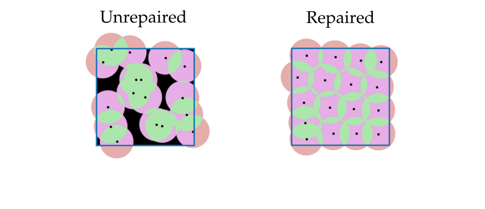
After BFGS is applied, we test that the agent is indeed covering the region. However, not every agent is repairable. In fact many will not be, for example, if the optimal solution for a cover is 15 circles a layout with 14 circles will never cover the region. Additionally, sometimes, even a layout with 15 circles may not cover the region after BFGS is applied. The agents which are not repairable are discarded. If a sufficient starting population is given this is not an issue. Finally, we remove circles which fully overlap with the agent and are redundant. See figure 1 to see a before and after of BFGS optimization on flat Euclidean space and Earth for an initial agent.
II.3 Fitness and Selection
The fitness function in this paper is determined by 3 factors: area of intersection between the circles and the outside of the region, area of self-intersection between the circles, and the number of circles. These factors are normalized to be between and so that it is easier to fine tune the fitness function. For a given agent, let , let , and . Then the fitness function is:
Here and are constants which determine the importance of each factor. As stated before, there is a degree of freedom when it come to the configurations. These parameters allow the user to reduce this degree of freedom. For example, if the least amount of self-intersection is desired, can be set to a very low number or even 0. The worst possible fitness is and the best is . In the flat algorithm , , . In the spherical algorithm , , . Note that this fitness function can be easily edited by others to incorporate the features they are interested in.
As for selection the bottom 20% of agents are deleted from the population. This number can be changed depending on the size of the initial population and the desired rate of convergence. I.e. higher initial populations can have higher deletion rates.
II.4 Crossover
In GAs there are multiple ways to construct crossover functions which vary on a problem by problem basis. In this case it is necessary to need to breed agents so that their desirable traits are conserved. Thus it does not make sense to randomly select circles from both of the parents and add them to the child as it will result in a configuration which is not similar to either parent. In particular, if a crossover function is not selected carefully, a consequence could be having all the circles on only half the region. Furthermore, this configuration will likely be irreparable. In essence, the aim is to construct a child which takes circles of parents which are locally close and selects one of them. In practice, this is done via Voronoi diagrams. Given points (sometimes called seeds), a Voronoi diagram on the plane is a partition of the plane into sub-regions such that each sub-region consists of points closer to than any other point.
The way the breeding works is by first constructing Voronoi diagrams for both parents. Then consider the Voronoi diagram from parent 1. Stack onto it the center points of parent 2. Iterate through the regions of the Voronoi diagram. If the region does not contain a point from parent 2, append to the circle list of child 1, the point which generated the current region. If instead the region contains points from parent 2 randomly select either all the points from parent 2 contained in the region, or the point from parent 1. Append these points to the circle list of child 1. The only difference in the spherical algorithm is the use of a spherical Voronoi function de Castro et al. (2009). See figure 2 for a pictorial description.
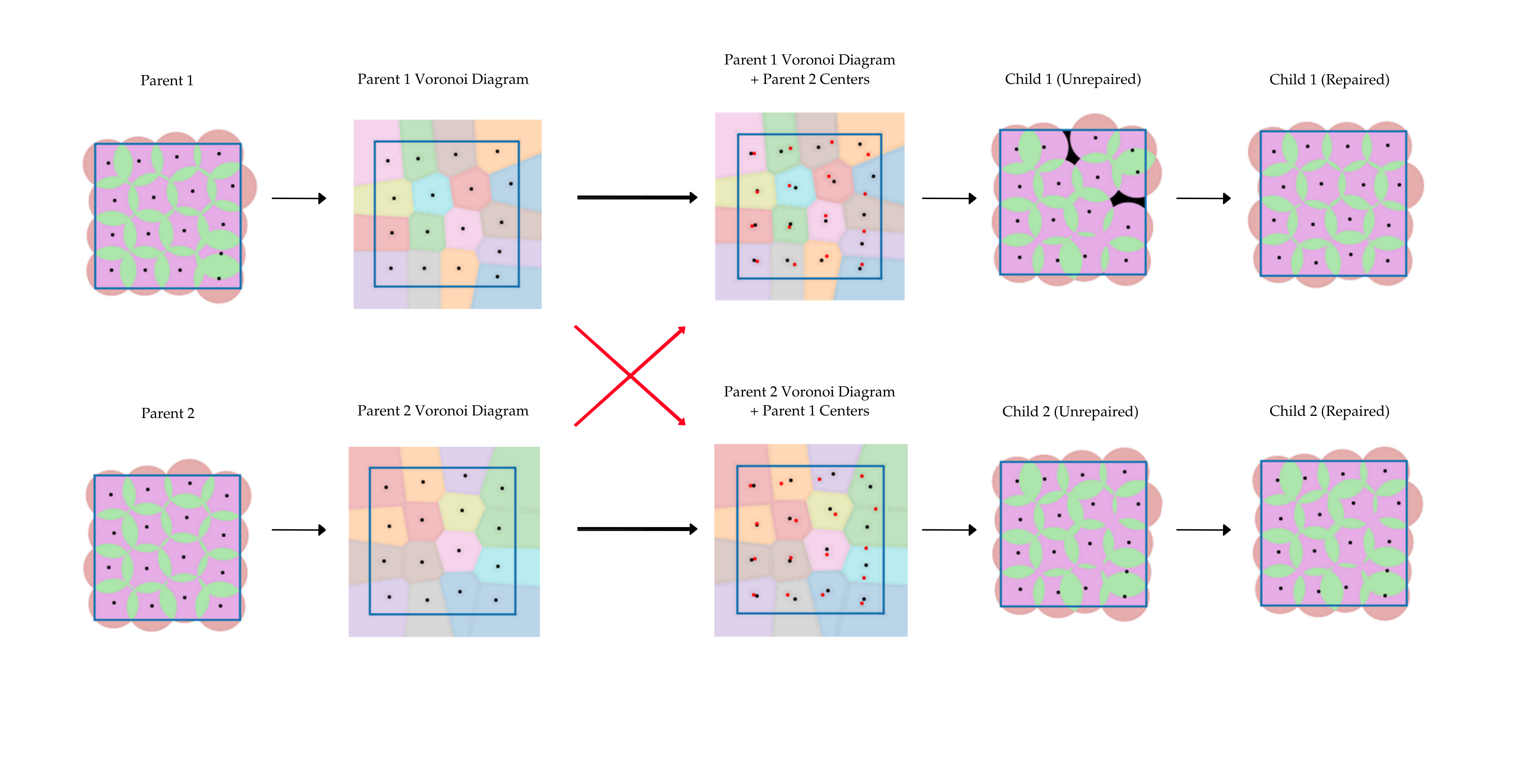
In this case we iterate through half the length of the population, randomly select 2 agents and breed them. Each bred pair produces 2 children. After iterating through the entire population the children and parents are added back into population and repaired as indicated in Algorithm 1.
II.5 Mutation
The final step in the algorithm is to “mutate” random agents in the population. There are 2 types of mutation, removing circles and moving circles. It isn’t effective to just remove random circles from the agent. Rather, it is better to remove the worst circles. There are 2 types of “worst” circles, circles which intersect the region the least and circles which self intersect the most. By self intersect the most, we mean the circle with the highest intersection between the circle list of the agent. The second type of mutation is moving a random circle by a random specified amount. The mutation rate for removal is .1 where as the mutation rate for moving the circle is . Again, these mutation rates can be changed based on the size of the initial population.
III Results
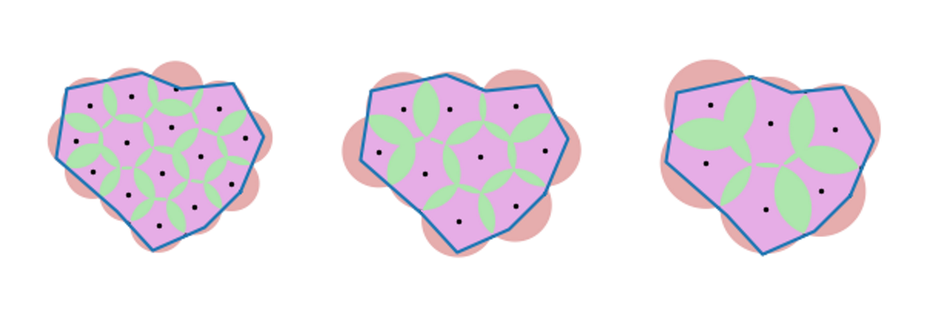
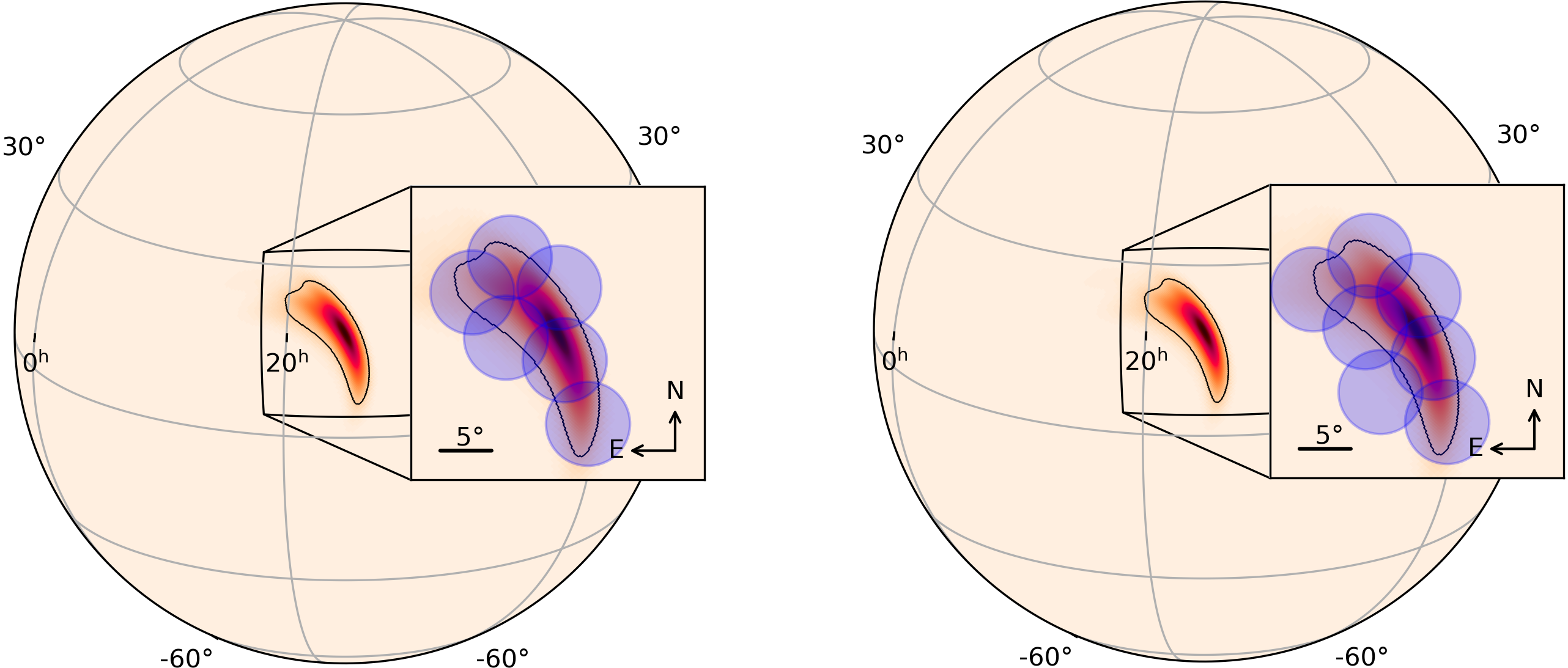
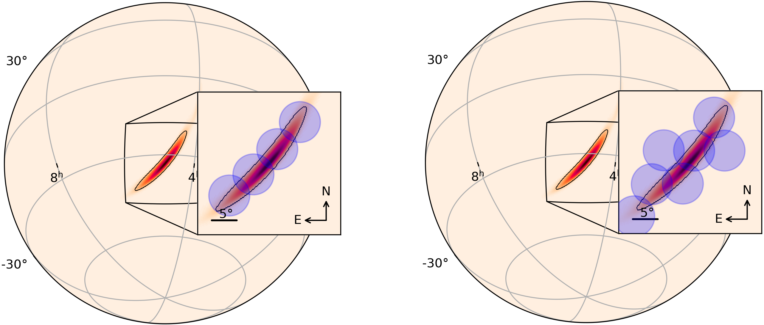
The algorithm presented above performs strongly given most polygons on flat space. Presented in figure 3 are a few configurations for 3 different radii for a randomly generated irregular polygon. Additionally, Fig. 4 compare the GA to the honeycomb method from Bartos et al. (2019). We also computed the tiling for 100 simulated LIGO sky localizations (obtained from Corley et al. (2019)) with both the hexagonal method and genetic algorithm method. The genetic algorithm performed better in 80% of the cases, while in the other 20% the genetic algorithm performed equally well. Overall, for skymaps requiring at least 10 tilings, the genetic algorithm presented a reduction in the number of tiles compared to the honeycomb method.
IV Conclusion
We developed an optimization strategy for the distribution of tilings in gravitational-wave follow-up observations using a genetic algorithm and a BFGS repair function. Compared to the standard “honeycomb” tiling strategy that is optimal in infinite flat surfaces, our method is superior in 80% of the cases, and in some cases it performs substantially better (e.g., Fig. 4).
We made the optimization algorithm available as a python code at https://github.com/kauii8school/GW-Localization-Tiling. This Github page contains three codes, Sphere_Light.py, Flat_GA.py, and Sphere_GA.py which correspond to the light version of the code, the Euclidean genetic algorithm, and the Spherical genetic algorithm respectively. The light version of the code is not a genetic algorithm but rather repeatedly uses BFGS optimization to try and cover a region. Specifically, if the user specifies a range of number of circles the program will start at the lower bound and try to cover the region. If it is unable to do so it will add more circles until either the upper bound is reached or the region is covered. If the program is able to cover the region this configuration will be considered as an “optimal covering”.
The optimization strategy developed here is applicable beyond gravitational-wave follow-up. It is a generalized solution for the equal circle covering problem on a spherical surface, and to higher dimensional polytopes. We also note that this algorithm can be easily extended to optimize for a range of circle radii rather than just a uniform radius.
For the optimization of tiling, we focused on a machine learning-based algorithm as they can also naturally incorporate other aspects of follow-up optimization, such as galaxy distributions, the temporal variations of the sources luminosity, and the follow-up observatories direction-dependent sensitivity. These elements are key in determining the best follow-up strategy. Our next step will be to generalize the algorithm presented here to account for these factors.
Acknowledgements.
The authors thank Tristano Di Girolamo and Ik Siong Heng for their useful feedback, and the University of Florida for their generous support.References
- Aasi et al. (2015) J. Aasi, B. P. Abbott, R. Abbott, T. Abbott, M. R. Abernathy, K. Ackley, C. Adams, T. Adams, P. Addesso, and et al., Classical and Quantum Gravity 32, 074001 (2015), ISSN 1361-6382, URL http://dx.doi.org/10.1088/0264-9381/32/7/074001.
- Acernese et al. (2014) F. Acernese, M. Agathos, K. Agatsuma, D. Aisa, N. Allemandou, A. Allocca, J. Amarni, P. Astone, G. Balestri, G. Ballardin, et al., Classical and Quantum Gravity 32, 024001 (2014), ISSN 1361-6382, URL http://dx.doi.org/10.1088/0264-9381/32/2/024001.
- Abbott et al. (2019) B. P. Abbott, R. Abbott, T. D. Abbott, S. Abraham, F. Acernese, et al., Phys. Rev. X 9, 031040 (2019), URL https://link.aps.org/doi/10.1103/PhysRevX.9.031040.
- Abbott et al. (2017a) B. P. Abbott, R. Abbott, T. D. Abbott, F. Acernese, K. Ackley, C. Adams, T. Adams, P. Addesso, R. X. Adhikari, V. B. Adya, et al., Phys. Rev. Lett. 119, 161101 (2017a), eprint 1710.05832.
- Abbott et al. (2017b) B. P. Abbott, R. Abbott, T. D. Abbott, F. Acernese, K. Ackley, C. Adams, T. Adams, P. Addesso, R. X. Adhikari, V. B. Adya, et al., ApJ Lett. 848, L12 (2017b), eprint 1710.05833.
- Abbott et al. (2016) B. P. Abbott, R. Abbott, T. D. Abbott, M. R. Abernathy, F. Acernese, K. Ackley, C. Adams, T. Adams, P. Addesso, R. X. Adhikari, et al., ApJ Lett. 826, L13 (2016), eprint 1602.08492.
- Bartos et al. (2013) I. Bartos, P. Brady, and S. Márka, Classical and Quantum Gravity 30, 123001 (2013), eprint 1212.2289.
- Murase and Bartos (2019) K. Murase and I. Bartos, Annual Review of Nuclear and Particle Science 69, 477 (2019), URL https://doi.org/10.1146/annurev-nucl-101918-023510.
- Goldstein et al. (2017) A. Goldstein, P. Veres, E. Burns, M. S. Briggs, R. Hamburg, D. Kocevski, C. A. Wilson-Hodge, R. D. Preece, S. Poolakkil, O. J. Roberts, et al., ApJ Lett. 848, L14 (2017), eprint 1710.05446.
- Savchenko et al. (2017) V. Savchenko, C. Ferrigno, E. Kuulkers, A. Bazzano, E. Bozzo, S. Brandt, J. Chenevez, T. J. L. Courvoisier, R. Diehl, A. Domingo, et al., ApJ Lett. 848, L15 (2017), eprint 1710.05449.
- Connaughton et al. (2016) V. Connaughton, E. Burns, A. Goldstein, L. Blackburn, M. S. Briggs, B. B. Zhang, J. Camp, N. Christensen, C. M. Hui, P. Jenke, et al., ApJ Lett. 826, L6 (2016), eprint 1602.03920.
- Savchenko et al. (2016) V. Savchenko, C. Ferrigno, S. Mereghetti, L. Natalucci, A. Bazzano, E. Bozzo, S. Brandt, T. J. L. Courvoisier, R. Diehl, L. Hanlon, et al., ApJ Lett. 820, L36 (2016), eprint 1602.04180.
- Troja et al. (2017) E. Troja, L. Piro, H. van Eerten, R. T. Wollaeger, M. Im, O. D. Fox, N. R. Butler, S. B. Cenko, T. Sakamoto, C. L. Fryer, et al., Nature (London) 551, 71 (2017), eprint 1710.05433.
- Coulter et al. (2017) D. A. Coulter, R. J. Foley, C. D. Kilpatrick, M. R. Drout, A. L. Piro, B. J. Shappee, M. R. Siebert, J. D. Simon, N. Ulloa, D. Kasen, et al., Science 358, 1556 (2017), eprint 1710.05452.
- Valenti et al. (2017) S. Valenti, D. J. Sand, S. Yang, E. Cappellaro, L. Tartaglia, A. Corsi, S. W. Jha, D. E. Reichart, J. Haislip, and V. Kouprianov, ApJ Lett. 848, L24 (2017), eprint 1710.05854.
- Evans et al. (2017) P. A. Evans, S. B. Cenko, J. A. Kennea, S. W. K. Emery, N. P. M. Kuin, O. Korobkin, R. T. Wollaeger, C. L. Fryer, K. K. Madsen, F. A. Harrison, et al., Science 358, 1565 (2017), eprint 1710.05437.
- Smartt et al. (2017) S. J. Smartt, T. W. Chen, A. Jerkstrand, M. Coughlin, E. Kankare, S. A. Sim, M. Fraser, C. Inserra, K. Maguire, K. C. Chambers, et al., Nature (London) 551, 75 (2017), eprint 1710.05841.
- Coughlin et al. (2019) M. W. Coughlin, T. Ahumada, S. Anand, K. De, M. J. Hankins, M. M. Kasliwal, L. P. Singer, E. C. Bellm, I. Andreoni, S. B. Cenko, et al., ApJ Lett. 885, L19 (2019), eprint 1907.12645.
- Antier et al. (2020) S. Antier, S. Agayeva, M. Almualla, S. Awiphan, A. Baransky, K. Barynova, S. Beradze, M. Blasek, M. Boer, O. Burkhonov, et al., arXiv preprint arXiv:2004.04277 (2020).
- Hosseinzadeh et al. (2019) G. Hosseinzadeh, P. S. Cowperthwaite, S. Gomez, V. A. Villar, M. Nicholl, R. Margutti, E. Berger, R. Chornock, K. Paterson, W. Fong, et al., ApJ Lett. 880, L4 (2019), eprint 1905.02186.
- Hallinan et al. (2017) G. Hallinan, A. Corsi, K. P. Mooley, K. Hotokezaka, E. Nakar, M. M. Kasliwal, D. L. Kaplan, D. A. Frail, S. T. Myers, T. Murphy, et al., Science 358, 1579 (2017), eprint 1710.05435.
- Adrián-Martínez et al. (2016) S. Adrián-Martínez, A. Albert, M. André, M. Anghinolfi, G. Anton, M. Ardid, J. J. Aubert, T. Avgitas, B. Baret, J. Barrios-Martí, et al., Phys. Rev. D 93, 122010 (2016), eprint 1602.05411.
- Albert et al. (2017a) A. Albert, M. André, M. Anghinolfi, G. Anton, M. Ardid, J. J. Aubert, T. Avgitas, B. Baret, J. Barrios-Martí, S. Basa, et al., Phys. Rev. D 96, 022005 (2017a), eprint 1703.06298.
- Albert et al. (2017b) A. Albert, M. André, M. Anghinolfi, M. Ardid, J. J. Aubert, J. Aublin, T. Avgitas, B. Baret, J. Barrios-Martí, S. Basa, et al., ApJ Lett. 850, L35 (2017b), eprint 1710.05839.
- Albert et al. (2019) A. Albert, M. André, M. Anghinolfi, M. Ardid, J. J. Aubert, et al., Astrophys. J. 870, 134 (2019), eprint 1810.10693.
- Abbott et al. (2020) B. Abbott, R. Abbott, T. Abbott, S. Abraham, F. Acernese, K. Ackley, C. Adams, R. Adhikari, V. Adya, C. Affeldt, et al., arXiv preprint arXiv:2001.01761 (2020).
- Bartos et al. (2011) I. Bartos, C. Finley, A. Corsi, and S. Márka, Phys. Rev. Lett. 107, 251101 (2011), eprint 1108.3001.
- Ghosh et al. (2017) S. Ghosh, D. Chatterjee, D. L. Kaplan, P. R. Brady, and A. Van Sistine, Publ. Astron. Soc. Pac. 129, 114503 (2017), eprint 1708.06723.
- Smartt et al. (2016) S. J. Smartt, K. C. Chambers, K. W. Smith, M. E. Huber, D. R. Young, E. Cappellaro, D. E. Wright, M. Coughlin, A. S. B. Schultz, L. Denneau, et al., MNRAS 462, 4094 (2016), eprint 1602.04156.
- Bartos et al. (2015) I. Bartos, A. P. S. Crotts, and S. Márka, ApJ Lett. 801, L1 (2015), eprint 1410.0677.
- Bartos et al. (2017) I. Bartos, Z. Haiman, Z. Marka, B. D. Metzger, N. C. Stone, and S. Marka, Nature Communications 8, 831 (2017), eprint 1701.02328.
- Greco et al. (2019) G. Greco, G. Stratta, E. Chassande-Mottin, M. W. Coughlin, F. Genova, M. Branchesi, M. Baumann, G. Hemming, L. Rei, S. Derriere, et al., PoS p. 031 (2019).
- Coughlin et al. (2019) M. W. Coughlin, S. Antier, D. Corre, K. Alqassimi, S. Anand, N. Christensen, R. J. Foley, N. Guessoum, T. M. Mikulski, M. A. Mualla, et al., arXiv preprint arXiv:1909.01244 (2019).
- Ducoin et al. (2020) J. Ducoin, D. Corre, N. Leroy, and E. Le Floch, Monthly Notices of the Royal Astronomical Society 492, 4768 (2020).
- Coughlin et al. (2018) M. W. Coughlin, D. Tao, M. L. Chan, D. Chatterjee, N. Christensen, S. Ghosh, G. Greco, Y. Hu, S. Kapadia, J. Rana, et al., MNRAS 478, 692 (2018), eprint 1803.02255.
- Ducoin et al. (2020) J. G. Ducoin, D. Corre, N. Leroy, and E. Le Floch, MNRAS 492, 4768 (2020), eprint 1911.05432.
- Bartos et al. (2018) I. Bartos, T. Di Girolamo, J. R. Gair, M. Hendry, I. S. Heng, T. B. Humensky, S. Márka, Z. Márka, C. Messenger, R. Mukherjee, et al., MNRAS 477, 639 (2018), eprint 1802.00446.
- Bartos et al. (2019) I. Bartos, K. R. Corley, N. Gupte, N. Ash, Z. Márka, and S. Márka, MNRAS 490, 3476 (2019), eprint 1908.09832.
- Bartos et al. (2014) I. Bartos, P. Veres, D. Nieto, V. Connaughton, B. Humensky, K. Hurley, S. Márka, P. Mészáros, R. Mukherjee, P. O’Brien, et al., MNRAS 443, 738 (2014), eprint 1403.6119.
- Seglar-Arroyo et al. (2019) M. Seglar-Arroyo, E. Bissaldi, A. Bulgarelli, A. Carosi, G. Cella, T. Di Girolamo, T. Gasparetto, G. Ghirlanda, B. Humensky, S. Inoue, et al., in 36th International Cosmic Ray Conference (ICRC2019) (2019), vol. 36 of International Cosmic Ray Conference, p. 790, eprint 1908.08393.
- Abdalla et al. (2019) H. Abdalla, R. Adam, F. Aharonian, F. Ait Benkhali, E. O. Angüner, M. Arakawa, C. Arcaro, C. Armand, H. Ashkar, M. Backes, et al., Nature 575, 464 (2019), URL https://doi.org/10.1038/s41586-019-1743-9.
- Acciari et al. (2019) V. A. Acciari, S. Ansoldi, L. A. Antonelli, A. Arbet Engels, D. Baack, A. Babić, B. Banerjee, U. Barres de Almeida, J. A. Barrio, J. Becerra González, et al., Nature 575, 455 (2019), URL https://doi.org/10.1038/s41586-019-1750-x.
- Croft et al. (2012) H. T. Croft, K. Falconer, and R. K. Guy, Unsolved problems in geometry: unsolved problems in intuitive mathematics, vol. 2 (Springer Science & Business Media, 2012).
- Melissen (1997) J. B. M. Melissen, PhD Thesis, Universiteit Utrecht (1997).
- Nurmela and Östergård (2000) K. J. Nurmela and P. R. Östergård (2000).
- Melissen and Schuur (1996) J. B. M. Melissen and P. C. Schuur, the electronic journal of combinatorics pp. R32–R32 (1996).
- Bánhelyi et al. (2015) B. Bánhelyi, E. Palatinus, and B. L. Lévai, Central European Journal of Operations Research 23, 815 (2015).
- Tarnai and Gáspár (1995) T. Tarnai and Z. Gáspár, Elemente der Mathematik 50, 167 (1995).
- Lengyel and Veres (1996) A. Lengyel and I. Veres, Competition essay, Technical University Budapest, Hungary (1996).
- Stoyan and Patsuk (2010) Y. G. Stoyan and V. Patsuk, Computational Optimization and Applications 46, 75 (2010).
- Deb (2005) K. Deb, Soft Computing 9, 236 (2005).
- Flores et al. (2016) J. J. Flores, J. Martínez, and F. Calderón, Soft Computing 20, 1521 (2016).
- Hifi and M’Hallah (2009) M. Hifi and R. M’Hallah, International Journal of Mathematics in Operational Research 1, 476 (2009).
- Avriel (2003) M. Avriel, Nonlinear programming: analysis and methods (Courier Corporation, 2003).
- de Castro et al. (2009) M. C. M. de Castro, S. L. R. Teillaud, and C. Wormser (2009).
- Corley et al. (2019) K. R. Corley, I. Bartos, L. P. Singer, A. R. Williamson, Z. Haiman, B. Kocsis, S. Nissanke, Z. Márka, and S. Márka, MNRAS 488, 4459 (2019), eprint 1902.02797.