EUROPEAN ORGANIZATION FOR NUCLEAR RESEARCH (CERN)

​​​ CERN-EP-2020-027 LHCb-PAPER-2020-002

Measurement

of $C\!P$-averaged observables

in the ${{B}^{0}}\!\rightarrow{{K}^{*0}}{\mu^{+}}{\mu^{-}}$ decay

LHCb collaboration

An angular analysis of the $B^{0}\rightarrow K^{*0}(\rightarrow{{K}^{+}}{{\pi}^{-}})\mu^{+}\mu^{-}$ decay is presented using a data set corresponding to an integrated luminosity of $4.7{\mbox{\,fb}^{-1}}$ of $pp$ collision data collected with the LHCb experiment. The full set of $C\!P$-averaged observables are determined in bins of the invariant mass squared of the dimuon system. Contamination from decays with the ${{K}^{+}}{{\pi}^{-}}$ system in an S-wave configuration is taken into account. The tension seen between the previous LHCb results and the Standard Model predictions persists with the new data. The precise value of the significance of this tension depends on the choice of theory nuisance parameters.

Submitted to Phys. Rev. Lett.

© 2024 CERN for the benefit of the LHCb collaboration, license CC BY 4.0 licence.

 

Decays mediated by the quark-level transition ${b}\!\rightarrow{s}\ell^{+}\ell^{-}$, where $\ell$ represents a lepton, have been the subject of intense recent study, as angular observables [1, 2, 3, 4, 5, 6, 7, 8], branching fractions [9, 8, 10, 11] and ratios of branching fractions between decays with different flavours of leptons [12, 13, 14, 15, 16] have been measured to be in tension with Standard Model (SM) predictions. Such decays are suppressed in the SM, as they proceed only through amplitudes that involve electroweak loop diagrams. The decays are sensitive to virtual contributions from new particles, which could have masses that are inaccessible to direct searches. The observed anomalies with respect to SM predictions can be explained consistently in New Physics models that introduce an additional vector or axial-vector contribution [17, 18, 19, 20, 21, 22, 23, 24, 25, 26, 27, 28, 29, 30, 31, 32, 33, 34, 35]. However, there is still considerable debate about whether some of the observations might instead be explained by hadronic uncertainties associated with the transition form factors, or by other long-distance effects [36, 37, 38, 39].

The LHCb collaboration presented a measurement of the angular observables of the ${{B}^{0}}\!\rightarrow{{K}^{*0}}{\mu^{+}\mu^{-}}$ decay in Ref. [1] and found that the data could be explained by modifying the real part of the vector coupling strength of the decays, conventionally denoted $\mathcal{R}e(C_{9})$. The analysis used the nuisance parameters from Ref. [40], implemented in the EOS software package described in Ref. [41], and found a 3.4 standard deviation ($\sigma$) tension with the SM value of $\mathcal{R}e(C_{9})$. The tension observed depends on the values of various SM nuisance parameters, including form-factor parameters and subleading corrections used to account for long-distance QCD interference effects with the charmonium modes. Using the Flavio software package [42], with its default SM nuisance parameters, gives a tension of $3.0\,\sigma$ with respect to the SM value of $\mathcal{R}e(C_{9})$ when fitting the angular observables from Ref. [1]. The nuisance parameters include a recent treatment of the subleading corrections [43, 44] that was not available at the time of the previous analysis.

This letter presents the most precise measurements of the complete set of $C\!P$-averaged angular observables in the decay ${{B}^{0}}\!\rightarrow{{K}^{*0}}{\mu^{+}}{\mu^{-}}$. The data set corresponds to an integrated luminosity of $4.7\text{\,fb}^{-1}$ of $p$ $p$ collisions collected with the LHCb experiment. The data were taken in the years 2011, 2012 and 2016, at centre-of-mass energies of $7$, $8$ and $13\text{\,Te\kern-1.00006ptV}$, respectively. The analysis uses the same technique as the analysis described in Ref. [1] but the data sample contains approximately twice as many ${B}^{0}$ decays, owing to the addition of the 2016 data. The ${b}{\overline{b}}$ production cross-section increases by roughly a factor of two between the Run 1 and 2016 datasets [45]. The same 2011 and 2012 (Run 1) data as in Ref. [1] are used in the present analysis. The results presented in this letter supersede the previous LHCb publication. The combination of the Run 1 data set with the 2016 data set requires a simultaneous angular fit to account for efficiency and reconstruction differences between years. Throughout this letter, ${K}^{*0}$ is used to refer to the ${{K}^{*}}(892)^{0}$ resonance and the inclusion of charge-conjugate processes is implied. The ${K}^{*0}$ meson is reconstructed through the decay ${{K}^{*0}}\rightarrow{{K}^{+}}{{\pi}^{-}}$.

The final state of the ${{B}^{0}}\!\rightarrow{{K}^{*0}}{\mu^{+}}{\mu^{-}}$ decay can be described by the invariant mass squared of the dimuon system, $q^{2}$, the invariant mass of the ${{K}^{+}}{{\pi}^{-}}$ system, and the three decay angles, $\vec{\Omega}=(\cos\theta_{l},\cos\theta_{K},\phi)$. The angle between the ${\mu^{+}}$ (${\mu^{-}}$) and the direction opposite to that of the ${{B}^{0}}$ (${{\kern 1.79993pt\overline{\kern-1.79993ptB}}{}^{0}}$) in the rest frame of the dimuon system is denoted $\theta_{l}$. The angle between the direction of the ${{K}^{+}}$ (${{K}^{-}}$) and the ${{B}^{0}}$ (${{\kern 1.79993pt\overline{\kern-1.79993ptB}}{}^{0}}$) in the rest frame of the ${{K}^{*0}}$ (${{\kern 1.79993pt\overline{\kern-1.79993ptK}}{}^{*0}}$) system is denoted $\theta_{K}$. The angle between the plane defined by the dimuon pair and the plane defined by the kaon and pion in the ${{B}^{0}}$ (${{\kern 1.79993pt\overline{\kern-1.79993ptB}}{}^{0}}$) rest frame is denoted $\phi$. A full description of the angular basis is provided in Ref. [46].

Following the definitions given in Refs. [47, 1], the $C\!P$-averaged angular distribution of the ${{B}^{0}}\!\rightarrow{{K}^{*0}}{\mu^{+}}{\mu^{-}}$ decay with the ${{K}^{+}}{{\pi}^{-}}$ system in a P-wave configuration can be written as

$$\begin{split}\left.\frac{1}{\mathrm{d}(\Gamma+\bar{\Gamma})/\mathrm{d}q^{2}}\,\frac{\mathrm{d}^{4}(\Gamma+\bar{\Gamma})}{\mathrm{d}{q^{2}}\,\mathrm{d}\vec{\Omega}}\right|_{\rm P}=\frac{9}{32\pi}\Big{[}&\tfrac{3}{4}(1-{F_{\rm L}})\sin^{2}\theta_{K}+{F_{\rm L}}\cos^{2}\theta_{K}\\ \phantom{\Big{[}}+&\tfrac{1}{4}(1-{F_{\rm L}})\sin^{2}\theta_{K}\cos 2\theta_{l}\\ \phantom{\Big{[}}-&{F_{\rm L}}\cos^{2}\theta_{K}\cos 2\theta_{l}+{S_{3}}\sin^{2}\theta_{K}\sin^{2}\theta_{l}\cos 2\phi\\ \phantom{\Big{[}}+&{S_{4}}\sin 2\theta_{K}\sin 2\theta_{l}\cos\phi+{S_{5}}\sin 2\theta_{K}\sin\theta_{l}\cos\phi\\ \phantom{\Big{[}}+&\tfrac{4}{3}{A_{\rm FB}}\sin^{2}\theta_{K}\cos\theta_{l}+{S_{7}}\sin 2\theta_{K}\sin\theta_{l}\sin\phi\\ +&{S_{8}}\sin 2\theta_{K}\sin 2\theta_{l}\sin\phi+{S_{9}}\sin^{2}\theta_{K}\sin^{2}\theta_{l}\sin 2\phi\Big{]}\,,\end{split}$$ (1)

where ${F_{\rm L}}$ is the fraction of the longitudinal polarisation of the ${K}^{*0}$ meson, ${A_{\rm FB}}$ is the forward-backward asymmetry of the dimuon system and $S_{i}$ are other $C\!P$-averaged observables [1]. The ${{K}^{+}}{{\pi}^{-}}$ system can also be in an S-wave configuration, which modifies the angular distribution to

$$\begin{split}\left.\frac{1}{\mathrm{d}(\Gamma+\bar{\Gamma})/\mathrm{d}q^{2}}\,\frac{\mathrm{d}^{4}(\Gamma+\bar{\Gamma})}{\mathrm{d}{q^{2}}\,\mathrm{d}\vec{\Omega}}\right|_{{\rm S}+{\rm P}}~{}=~{}&(1-F_{\rm S})\left.\frac{1}{\mathrm{d}(\Gamma+\bar{\Gamma})/\mathrm{d}q^{2}}\,\frac{\mathrm{d}^{4}(\Gamma+\bar{\Gamma})}{\mathrm{d}{q^{2}}\,\mathrm{d}\vec{\Omega}}\right|_{\rm P}\\ &+\frac{3}{16\pi}F_{\rm S}\sin^{2}\theta_{l}\\ &+\frac{9}{32\pi}(S_{11}+S_{13}\cos 2\theta_{l})\cos\theta_{K}\\ &+\frac{9}{32\pi}(S_{14}\sin 2\theta_{l}+S_{15}\sin\theta_{l})\sin\theta_{K}\cos\phi\\ &+\frac{9}{32\pi}(S_{16}\sin\theta_{l}+S_{17}\sin 2\theta_{l})\sin\theta_{K}\sin\phi\,,\end{split}$$ (2)

where $F_{\rm S}$ denotes the S-wave fraction and the coefficients $S_{11}$, $S_{13}$–$S_{17}$ arise from interference between the S- and P-wave amplitudes. Throughout this letter, $F_{\rm S}$ and the interference terms between the S- and P-wave are treated as nuisance parameters.

Additional sets of observables, for which the leading ${{B}^{0}}\rightarrow{{K}^{*0}}$ form-factor uncertainties cancel, can be built from $F_{\rm L}$, $A_{\rm FB}$ and $S_{3}$–$S_{9}$. Examples of such optimised observables include the $P^{(\prime)}_{i}$ series of observables [48]. The notation used in this letter again follows Ref. [1], for example $P_{5}^{\prime}=S_{5}/\sqrt{F_{\rm L}(1-F_{\rm L})}$.

The LHCb detector is a single-arm forward spectrometer covering the pseudorapidity range $2<\eta<5$, described in detail in Refs. [49, 50]. The detector includes a vertex detector surrounding the proton-proton interaction region, tracking stations on either side of a dipole magnet, ring-imaging Cherenkov (RICH) detectors, electromagnetic and hadronic calorimeters and muon chambers.

Simulated signal events are used in this analysis to determine the impact of the detector geometry, trigger, reconstruction and candidate selection on the angular distribution of the signal. The simulation is produced using the software described in Refs. [51, *Sjostrand:2007gs, 53, 54, 55, 56, *Agostinelli:2002hh, 58]. Corrections derived from the data are applied to the simulation to account for mismodelling of the charge multiplicity of the event, ${B}^{0}$ momentum spectrum and ${B}^{0}$ vertex quality. Similarly, the simulated particle identification (PID) performance is corrected to match that determined from control samples selected from the data [59, 60].

The online event selection is performed by a trigger, which comprises a hardware stage, based on information from the calorimeter and muon systems, followed by a software stage that applies a full event reconstruction [61]. Offline, signal candidates are formed from a pair of oppositely charged tracks that are identified as muons, combined with a ${K}^{*0}$ candidate.

The distribution of the reconstructed ${K}^{+}$ ${\pi}^{-}$ $\mu^{+}\mu^{-}$ invariant mass, $m({{K}^{+}}{{\pi}^{-}}{\mu^{+}\mu^{-}})$, is used to discriminate signal from background. This distribution is fitted simultaneously with the three decay angles. The distribution of the reconstructed ${{K}^{+}}{{\pi}^{-}}$ mass, $m({{K}^{+}}{{\pi}^{-}})$, depends on the ${{K}^{+}}{{\pi}^{-}}$ angular-momentum configuration and is used to constrain the S-wave fraction. The analysis procedure is cross-checked by performing a fit of the ${b}\rightarrow{{c}{\overline{c}}}{s}$ tree-level decay ${{B}^{0}}\!\rightarrow{{J\mskip-3.0mu/\mskip-2.0mu\psi}}{{K}^{*0}}$, with ${{J\mskip-3.0mu/\mskip-2.0mu\psi}}\!\rightarrow{\mu^{+}\mu^{-}}$, which results in the same final-state particles. Hereafter, the ${{B}^{0}}\!\rightarrow{{J\mskip-3.0mu/\mskip-2.0mu\psi}}(\rightarrow{\mu^{+}\mu^{-}}){{K}^{*0}}$ decay and the equivalent decay via the $\psi{(2S)}$ resonance are denoted by ${{B}^{0}}\!\rightarrow{{J\mskip-3.0mu/\mskip-2.0mu\psi}}{{K}^{*0}}$ and ${{B}^{0}}\!\rightarrow{\psi{(2S)}}{{K}^{*0}}$, respectively.

Two types of backgrounds are considered: combinatorial background, where the selected particles do not originate from a single ${b}$-hadron decay; and peaking backgrounds, where a single decay is selected but with some of the final-state particles misidentified. The combinatorial background is distributed smoothly in $m({{K}^{+}}{{\pi}^{-}}{\mu^{+}\mu^{-}})$, whereas the peaking backgrounds can accumulate in specific regions of the reconstructed mass. In addition, the decays ${{B}^{0}}\!\rightarrow{{J\mskip-3.0mu/\mskip-2.0mu\psi}}{{K}^{*0}}$, ${{B}^{0}}\!\rightarrow{\psi{(2S)}}{{K}^{*0}}$ and ${{B}^{0}}\!\rightarrow\phi(1020)(\rightarrow{\mu^{+}\mu^{-}}){{K}^{*0}}$ are removed by rejecting events with $q^{2}$ in the ranges $8.0<{q^{2}}<11.0\text{\,Ge\kern-1.00006ptV}^{2}\!/c^{4}$, $12.5<{q^{2}}<15.0\text{\,Ge\kern-1.00006ptV}^{2}\!/c^{4}$ or $0.98<{q^{2}}<1.10\text{\,Ge\kern-1.00006ptV}^{2}\!/c^{4}$.

The criteria used to select candidates from the Run 1 data are the same as those described in Ref. [1]. The selection of the 2016 data follows closely that of the Run 1 data. Candidates are required to have $5170<m({{K}^{+}}{{\pi}^{-}}{\mu^{+}\mu^{-}})<5700\text{\,Me\kern-1.00006ptV\!/}c^{2}$ and $795.9<m({{K}^{+}}{{\pi}^{-}})<995.9\text{\,Me\kern-1.00006ptV\!/}c^{2}$. The four tracks of the final-state particles are required to have significant impact parameter (IP) with respect to all primary vertices (PVs) in the event. The tracks are fitted to a common vertex, which is required to be of good quality. The IP of the ${B}^{0}$ candidate is required to be small with respect to one of the PVs. The vertex of the ${B}^{0}$ candidate is required to be significantly displaced from the same PV. The angle between the reconstructed ${B}^{0}$ momentum and the vector connecting this PV to the reconstructed ${B}^{0}$ decay vertex, $\theta_{\rm DIRA}$, is also required to be small. To avoid the same track being used to construct more than one of the final state particles, the opening angle between every pair of tracks is required to be larger than 1 mrad.

Combinatorial background is reduced further using a boosted decision tree (BDT) algorithm [62, 63]. The BDT is trained entirely on data with ${{B}^{0}}\!\rightarrow{{J\mskip-3.0mu/\mskip-2.0mu\psi}}{{K}^{*0}}$ candidates used as a proxy for the signal and candidates from the upper-mass sideband $5350<m({{K}^{+}}{{\pi}^{-}}{\mu^{+}\mu^{-}})<7000\text{\,Me\kern-1.00006ptV\!/}c^{2}$ used as a proxy for the background. The training uses a cross-validation technique [64] and is performed separately for the Run 1 and 2016 data sets. The input variables used are the reconstructed ${B}^{0}$ decay-time and vertex-fit quality, the momentum and transverse momentum of the ${B}^{0}$ candidate, $\theta_{\rm DIRA}$, PID information from the RICH detectors and the muon system, and variables describing the isolation of the final-state tracks [65]. Variables are only used in the BDT if they do not have a strong correlation with the decay angles or $q^{2}$. A requirement is placed on the BDT output to maximise the signal significance. This requirement rejects more than $97\%$ of the remaining combinatorial background, while retaining more than $85\%$ of the signal. The signal efficiency of the BDT is uniform in the $m({{K}^{+}}{{\pi}^{-}}{\mu^{+}\mu^{-}})$ and $m({{K}^{+}}{{\pi}^{-}})$ distributions.

Peaking backgrounds from ${{B}^{0}_{s}}\!\rightarrow\phi(1020)(\rightarrow{{K}^{+}}{{K}^{-}}){\mu^{+}\mu^{-}}$, ${{\mathchar 28931\relax}^{0}_{b}}\!\rightarrow{p}{{K}^{-}}{\mu^{+}\mu^{-}}$, ${{B}^{0}}\!\rightarrow{{J\mskip-3.0mu/\mskip-2.0mu\psi}}{{K}^{*0}}$, ${{B}^{0}}\!\rightarrow{\psi{(2S)}}{{K}^{*0}}$ and ${{\kern 1.79993pt\overline{\kern-1.79993ptB}}{}^{0}}\!\rightarrow{{\kern 1.79993pt\overline{\kern-1.79993ptK}}{}^{*0}}{\mu^{+}}{\mu^{-}}$ decays are considered, where the latter constitutes a background if the kaon from the ${\kern 1.79993pt\overline{\kern-1.79993ptK}}{}^{*0}$ decay is misidentified as the pion and vice versa. In each case, at least one particle needs to be misidentified for the decay to be reconstructed as a signal candidate. Vetoes to reduce these peaking backgrounds are formed by placing requirements on the invariant mass of the candidates, recomputed with the relevant change in the particle mass hypotheses, and by using PID information. In addition, in order to avoid having a strongly peaking contribution to the $\cos\theta_{K}$ angular distribution in the upper mass sideband, ${{{B}^{+}}}\!\rightarrow{{K}^{+}}{\mu^{+}}{\mu^{-}}$ candidates with ${{K}^{+}}{\mu^{+}\mu^{-}}$ invariant mass within $60\text{\,Me\kern-1.00006ptV\!/}c^{2}$ of the ${{B}^{+}}$ mass are removed. The background from $b$-hadron decays with two hadrons misidentified as muons is negligible. The signal efficiency and residual peaking backgrounds are estimated using simulated events. The vetoes remove a negligible amount of signal. The largest residual backgrounds are from ${{\kern 1.79993pt\overline{\kern-1.79993ptB}}{}^{0}}\!\rightarrow{{\kern 1.79993pt\overline{\kern-1.79993ptK}}{}^{*0}}{\mu^{+}}{\mu^{-}}$, ${{\mathchar 28931\relax}^{0}_{b}}\!\rightarrow p{{K}^{-}}{\mu^{+}\mu^{-}}$ and ${{B}^{0}_{s}}\!\rightarrow\phi(1020)(\rightarrow{{K}^{+}}{{K}^{-}}){\mu^{+}\mu^{-}}$ decays, at the level of 1% or less of the expected signal yield. This is sufficiently small such that these backgrounds are neglected in the angular analysis and are considered only as sources of systematic uncertainty.

For every $q^{2}$ bin, a fit is performed in both the standard and the optimised basis. For each basis, four data sets are fit simultaneously: the $m({{K}^{+}}{{\pi}^{-}}{\mu^{+}\mu^{-}})$ and angular distributions of candidates in the Run 1 data; the equivalent distributions for the 2016 data; and the $m({{K}^{+}}{{\pi}^{-}})$ distributions of candidates in the Run 1 and the 2016 data sets. The signal fraction is shared between the two data sets from each data-taking period. The $C\!P$-averaged angular observables and the S-wave fraction are shared between all data sets. The fitted probability density functions (PDFs) are of an identical form to those of Ref. [1], as are the $q^{2}$ bins used. In addition to the narrow ${q^{2}}$ bins, results are obtained for the wider bins $1.1<{q^{2}}<6.0\text{\,Ge\kern-1.00006ptV}^{2}\!/c^{4}$ and $15.0<{q^{2}}<19.0\text{\,Ge\kern-1.00006ptV}^{2}\!/c^{4}$.

The angular distribution of the signal is described using Eq. (1). The $P_{i}^{(\prime)}$ observables are determined by reparameterising Eq. (1) using a basis comprising $F_{\rm L}$, $P_{1,2,3}$ and $P_{4,5,6,8}^{\prime}$. The angular distribution is multiplied by an acceptance model used to account for the effect of the reconstruction and candidate selection. The acceptance function is parameterised in four dimensions, according to

$${\varepsilon}(\cos\theta_{l},\cos\theta_{K},\phi,q^{2}) =\sum_{ijmn}c_{ijmn}L_{i}(\cos\theta_{l})L_{j}(\cos\theta_{K})L_{m}(\phi)L_{n}(q^{2})\,,$$ (3)

where the terms $L_{h}(x)$ denote Legendre polynomials of order $h$ and the values of the angles and $q^{2}$ are rescaled to the range $-1<x<+1$ when evaluating the polynomials. For the $\cos\theta_{l}$, $\cos\theta_{K}$ and $\phi$ angles, the sum in Eq. (3) encompasses $L_{h}(x)$ up to fourth, fifth and sixth order, respectively. The $q^{2}$ parameterisation comprises $L_{h}(x)$ up to fifth order. Simulation indicates that the acceptance function can be assumed to be flat across $m({{K}^{+}}{{\pi}^{-}})$. The coefficients $c_{ijmn}$ are determined using a principal moment analysis of simulated ${{B}^{0}}\!\rightarrow{{K}^{*0}}{\mu^{+}}{\mu^{-}}$ decays. As all of the relevant kinematic variables needed to describe the decay are used in this parameterisation, the acceptance function does not depend on the decay model used in the simulation.

In the narrow $q^{2}$ bins, the acceptance is taken to be constant across each bin and is included in the fit by multiplying Eq. (2) by the acceptance function evaluated with the value of $q^{2}$ fixed at the bin centre. In the wider $q^{2}$ bins, the shape of the acceptance can vary significantly across the bin. In the likelihood, candidates are therefore weighted by the inverse of the acceptance function and parameter uncertainties are obtained using a bootstrapping technique [66].

The background angular distribution is modelled with second-order polynomials in $\cos\theta_{l}$, $\cos\theta_{K}$ and $\phi$, with the angular coefficients allowed to vary in the fit. This angular distribution is assumed to factorise in the three decay angles, which is confirmed to be the case for candidates in the upper mass sideband of the data.

The $m({{K}^{+}}{{\pi}^{-}}{\mu^{+}\mu^{-}})$ distribution of the signal candidates is modelled using the sum of two Gaussian functions with a common mean, each with a power-law tail on the low mass side. The parameters describing the signal mass shape are determined from a fit to the ${{B}^{0}}\!\rightarrow{{J\mskip-3.0mu/\mskip-2.0mu\psi}}{{K}^{*0}}$ decay in the data and are subsequently fixed when fitting the ${{B}^{0}}\!\rightarrow{{K}^{*0}}{\mu^{+}}{\mu^{-}}$ candidates. For each of the $q^{2}$ bins, a scale factor that is determined from simulation is included to account for the difference in resolution between the ${{B}^{0}}\!\rightarrow{{J\mskip-3.0mu/\mskip-2.0mu\psi}}{{K}^{*0}}$ and ${{B}^{0}}\!\rightarrow{{K}^{*0}}{\mu^{+}}{\mu^{-}}$ decay modes. A component is included in the ${{B}^{0}}\!\rightarrow{{J\mskip-3.0mu/\mskip-2.0mu\psi}}{{K}^{*0}}$ fit to account for ${{\kern 1.79993pt\overline{\kern-1.79993ptB}}{}^{0}_{s}}\!\rightarrow{{J\mskip-3.0mu/\mskip-2.0mu\psi}}{{K}^{*0}}$ decays, which are at the level of $\sim 1\%$ of the ${{B}^{0}}\!\rightarrow{{J\mskip-3.0mu/\mskip-2.0mu\psi}}{{K}^{*0}}$ signal yield. The background from the equivalent Cabibbo-suppressed penguin decay, ${{\kern 1.79993pt\overline{\kern-1.79993ptB}}{}^{0}_{s}}\!\rightarrow{{K}^{*0}}{\mu^{+}\mu^{-}}$ [67], is negligible and is ignored in the fit of the signal decay. The combinatorial background is described well by an exponential distribution in $m({{K}^{+}}{{\pi}^{-}}{\mu^{+}\mu^{-}})$.

The ${{K}^{*0}}$ signal component in the $m({{K}^{+}}{{\pi}^{-}})$ distribution is modelled using a relativistic Breit-Wigner function for the P-wave component and the LASS parameterisation [68] for the S-wave component. The combinatorial background is described by a linear function in $m({{K}^{+}}{{\pi}^{-}})$.

The decay ${{B}^{0}}\!\rightarrow{{J\mskip-3.0mu/\mskip-2.0mu\psi}}{{K}^{*0}}$ is used to cross-check the analysis procedure in the region $8.0<{q^{2}}<11.0\text{\,Ge\kern-1.00006ptV}^{2}\!/c^{4}$. This decay is selected in the data with negligible background contamination. The angular structure has been determined by measurements made by the BaBar, Belle and LHCb collaborations [69, 70, 71]. The ${{B}^{0}}\!\rightarrow{{J\mskip-3.0mu/\mskip-2.0mu\psi}}{{K}^{*0}}$ angular observables obtained from the Run 1 and 2016 LHCb data, using the acceptance correction derived as described above, are in good agreement with these previous measurements.

Figure 1 shows the projection of the fitted PDF on the ${K}^{+}$ ${\pi}^{-}$ $\mu^{+}\mu^{-}$ mass distribution. The ${{B}^{0}}\!\rightarrow{{K}^{*0}}{\mu^{+}}{\mu^{-}}$ yield, integrated over the $q^{2}$ ranges $0.10<{q^{2}}<0.98\text{\,Ge\kern-1.00006ptV}^{2}\!/c^{4}$, $1.1<{q^{2}}<8.0\text{\,Ge\kern-1.00006ptV}^{2}\!/c^{4}$, $11.0<{q^{2}}<12.5\text{\,Ge\kern-1.00006ptV}^{2}\!/c^{4}$ and $15.0<{q^{2}}<19.0\text{\,Ge\kern-1.00006ptV}^{2}\!/c^{4}$, is determined to be $2398\pm 57$ for the Run 1 data, and $2187\pm 53$ for the 2016 data.

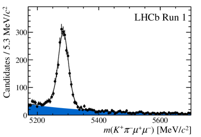
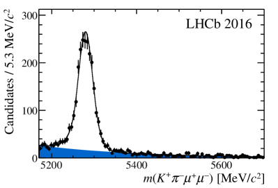
Figure 1: The ${{K}^{+}}{{\pi}^{-}}{\mu^{+}\mu^{-}}$ mass distribution of candidates with $0.1<{q^{2}}<19.0\text{\,Ge\kern-1.00006ptV}^{2}/c^{4}$, excluding the $\phi(1020)$ and charmonium regions, for the (left) Run 1 data and (right) 2016 data. The background is indicated by the shaded region.

Pseudoexperiments, generated using the results of the best fit to data, are used to assess the bias and coverage of the fit. The majority of observables have a bias of less than 10% of their statistical uncertainty, with the largest bias being 17%, and all observables have an uncertainty estimate within 10% of the true uncertainty. The biases are driven by boundary effects in the observables. The largest effect comes from requiring that $F_{\rm S}\geq 0$, which can bias $F_{\rm S}$ to larger values. This can then result in a bias in the P-wave observables (see Eq. 2). The statistical uncertainty is corrected to account for any under- or over-coverage and a systematic uncertainty equal to the size of the observed bias is assigned.

The size of other sources of systematic uncertainty is estimated using pseudoexperiments, in which one or more parameters are varied and the angular observables are determined with and without this variation. The systematic uncertainty is then taken as the difference between the two models. The pseudoexperiments are generated with signal yields many times larger than the data, in order to render statistical fluctuations negligible.

The size of the total systematic uncertainty varies depending on the angular observable and the $q^{2}$ bin. The majority of observables in both the $S_{i}$ and $P^{(\prime)}_{i}$ basis have a total systematic uncertainty between 5% and 25% of the statistical uncertainty. For $F_{\rm L}$, the systematic uncertainty tends to be larger, typically between 20% and 50%. The systematic uncertainties are given in Table 3 of the Supplemental Material.

The dominant systematic uncertainties arise from the peaking backgrounds that are neglected in the analysis, the bias correction, and, for the narrow $q^{2}$ bins, from the uncertainty associated with evaluating the acceptance at a fixed point in $q^{2}$. For the peaking backgrounds, the systematic uncertainty is evaluated by injecting additional candidates, drawn from the angular distributions of the background modes, into the pseudoexperiment data. The systematic uncertainty for the bias correction is determined directly from the pseudoexperiments used to validate the fit. The systematic uncertainty from the variation of the acceptance with $q^{2}$ is determined by moving the point in $q^{2}$ at which the acceptance is evaluated to halfway between the bin centre and the upper or the lower edge. The largest deviation is taken as the systematic uncertainty. Examples of further sources of systematic uncertainty investigated include the $m({{K}^{+}}{{\pi}^{-}})$ lineshape for the S-wave contribution, the assumption that the acceptance function is flat across the $m({{K}^{+}}{{\pi}^{-}})$ mass, the effect of the ${{{B}^{+}}}\!\rightarrow{{K}^{+}}{\mu^{+}}{\mu^{-}}$ veto on the angular distribution of the background and the order of polynomial used for the background parameterisation. These sources make a negligible contribution to the total uncertainty. With respect to the analysis of Ref. [1], the systematic uncertainty from residual differences between data and simulation is significantly reduced, owing to an improved decay model for ${{B}^{0}}\!\rightarrow{{J\mskip-3.0mu/\mskip-2.0mu\psi}}{{K}^{*0}}$ decays [70].

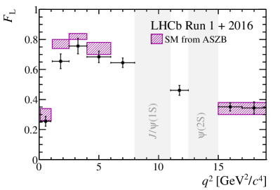
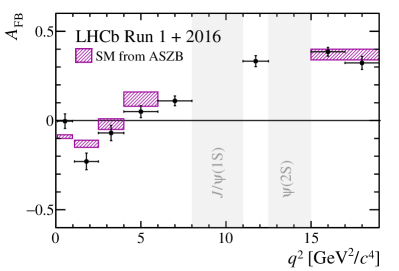
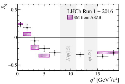
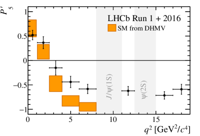
Figure 2: Results for the $C\!P$-averaged angular observables $F_{\rm L}$, $A_{\rm FB}$, $S_{5}$ and $P_{5}^{\prime}$ in bins of $q^{2}$. The data are compared to SM predictions based on the prescription of Refs. [44, 43], with the exception of the $P_{5}^{\prime}$ distribution, which is compared to SM predictions based on Refs. [72, 73].

The $C\!P$-averaged observables $F_{\rm L}$, $A_{\rm FB}$, $S_{5}$ and $P^{\prime}_{5}$ that are obtained from the $S_{i}$ and $P_{i}^{(\prime)}$ fits are shown together with their respective SM predictions in Fig. 2. The results for all observables are given in Figs. 3 and 4 and Tables 1 and 2 of the Supplemental Material. In addition, the statistical correlation between the observables is provided in Tables 4–23. The SM predictions are based on the prescription of Ref. [44], which combines light-cone sum rule calculations [43], valid in the low-$q^{2}$ region, with lattice determinations at high $q^{2}$ [74, 75] to yield more precise determinations of the form factors over the full $q^{2}$ range. For the $P^{(\prime)}_{i}$ observables, predictions from Ref. [72] are shown using form factors from Ref. [73]. These predictions are restricted to the region ${q^{2}}<8.0\text{\,Ge\kern-1.00006ptV}^{2}\!/c^{4}$. The results from Run 1 and the 2016 data are in excellent agreement. A stand-alone fit to the Run 1 data reproduces exactly the central values of the observables obtained in Ref. [1].

Considering the observables individually, the results are largely in agreement with the SM predictions. The local discrepancy in the $P^{\prime}_{5}$ observable in the $4.0<q^{2}<6.0\text{\,Ge\kern-1.00006ptV}^{2}\!/c^{4}$ and $6.0<q^{2}<8.0\text{\,Ge\kern-1.00006ptV}^{2}\!/c^{4}$ bins reduces from the 2.8 and $3.0\,\sigma$ observed in Ref. [1] to 2.5 and $2.9\,\sigma$. However, as discussed below, the overall tension with the SM is observed to increase mildly.

Using the Flavio software package [42], a fit of the angular observables is performed varying the parameter $\mathcal{R}e(C_{9})$. The default Flavio SM nuisance parameters are used, including form-factor parameters and subleading corrections to account for long-distance QCD interference effects with the charmonium decay modes [43, 44]. The same $q^{2}$ bins as in Ref. [1] are included. The $3.0\,\sigma$ discrepancy with respect to the SM value of $\mathcal{R}e(C_{9})$ obtained with the Ref. [1] data set changes to $3.3\,\sigma$ with the data set used here. The best fit to the angular distribution is obtained with a shift in the SM value of $\mathcal{R}e(C_{9})$ by $-0.99^{+0.25}_{-0.21}$. The tension observed in any such fit will depend on the effective coupling(s) varied, the handling of the SM nuisance parameters and the $q^{2}$ bins that are included in the fit. For example, the $6.0<{q^{2}}<8.0\text{\,Ge\kern-1.00006ptV}^{2}\!/c^{4}$ bin is known to be associated with larger theoretical uncertainties [47]. Neglecting this bin, a Flavio fit gives a tension of $2.4\,\sigma$ using the observables from Ref. [1] and $2.7\,\sigma$ tension with the measurements reported here.

In summary, using $4.7{\mbox{\,fb}^{-1}}$ of $pp$ collision data collected with the LHCb experiment during the years 2011, 2012 and 2016, a complete set of $C\!P$-averaged angular observables has been measured for the ${{B}^{0}}\!\rightarrow{{K}^{*0}}{\mu^{+}}{\mu^{-}}$ decay. These are the most precise measurements of these quantities to date.

1 Results

The values of $S_{3}$, $S_{4}$ and $S_{7}$–$S_{9}$ obtained from the simultaneous fit are shown in Fig. 3. The data are compared to theoretical predictions based on the prescription of Ref. [44]. The predictions combine light-cone sum rule calculations [43] with lattice determinations [74, 75] of the ${{B}^{0}}\rightarrow{{K}^{*0}}$ form factors. Figure 4 shows the values of the optimised observables, $P_{i}^{(\prime)}$, obtained from the fit. The data are compared to predictions based on the prescription in Ref. [72]. These predictions use form factors from Ref. [73]. The values of the observables in the standard and optimised basis are given in Tables 1 and 2, respectively. The statistical correlation between the observables in each $q^{2}$ bin is provided in Tables 4–13 and Tables 14–23.

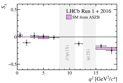
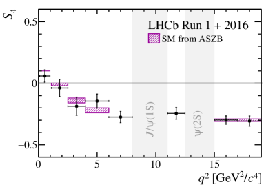
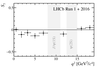
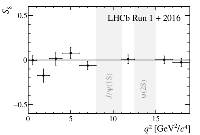
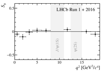
Figure 3: Results for the $C\!P$-averaged angular observables $S_{3}$, $S_{4}$ and $S_{7}$–$S_{9}$ in bins of $q^{2}$. The data are compared to SM predictions based on the prescription of Refs. [44, 43].

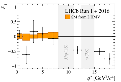
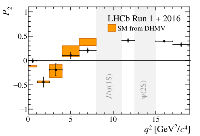
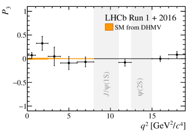
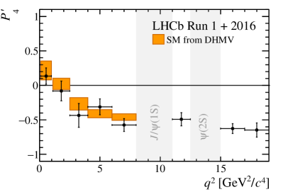
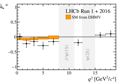
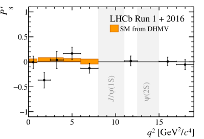
Figure 4: Results for the optimised angular observables $P_{1}$–$P_{3}$, $P_{4}^{\prime}$, $P_{6}^{\prime}$ and $P_{8}^{\prime}$ in bins of $q^{2}$. The data are compared to SM predictions based on Refs. [72, 73].

Table 1: Results for the $C\!P$-averaged observables $F_{\rm L}$, $A_{\rm FB}$ and $S_{3}$–$S_{9}$. The first uncertainties are statistical and the second systematic.

$0.10<q^{2}<0.98\text{\,Ge\kern-0.80005ptV}^{2}\!/c^{4}$
$F_{\rm L}$	$0.255\pm 0.032\pm 0.007$
$S_{3}$	$0.034\pm 0.044\pm 0.003$
$S_{4}$	$0.059\pm 0.050\pm 0.004$
$S_{5}$	$0.227\pm 0.041\pm 0.008$
$A_{\rm FB}$	$-0.004\pm 0.040\pm 0.004$
$S_{7}$	$0.006\pm 0.042\pm 0.002$
$S_{8}$	$-0.003\pm 0.051\pm 0.001$
$S_{9}$	$-0.055\pm 0.041\pm 0.002$

$1.1<q^{2}<2.5\text{\,Ge\kern-0.80005ptV}^{2}\!/c^{4}$
$F_{\rm L}$	$0.655\pm 0.046\pm 0.017$
$S_{3}$	$-0.107\pm 0.052\pm 0.003$
$S_{4}$	$-0.038\pm 0.070\pm 0.011$
$S_{5}$	$0.174\pm 0.060\pm 0.007$
$A_{\rm FB}$	$-0.229\pm 0.046\pm 0.009$
$S_{7}$	$-0.107\pm 0.063\pm 0.004$
$S_{8}$	$-0.174\pm 0.075\pm 0.002$
$S_{9}$	$-0.112\pm 0.054\pm 0.005$

$2.5<q^{2}<4.0\text{\,Ge\kern-0.80005ptV}^{2}\!/c^{4}$
$F_{\rm L}$	$0.756\pm 0.047\pm 0.023$
$S_{3}$	$0.020\pm 0.053\pm 0.002$
$S_{4}$	$-0.187\pm 0.074\pm 0.008$
$S_{5}$	$-0.064\pm 0.068\pm 0.010$
$A_{\rm FB}$	$-0.070\pm 0.043\pm 0.006$
$S_{7}$	$-0.066\pm 0.065\pm 0.004$
$S_{8}$	$0.016\pm 0.074\pm 0.002$
$S_{9}$	$-0.012\pm 0.055\pm 0.003$

$4.0<q^{2}<6.0\text{\,Ge\kern-0.80005ptV}^{2}\!/c^{4}$
$F_{\rm L}$	$0.684\pm 0.035\pm 0.015$
$S_{3}$	$0.014\pm 0.038\pm 0.003$
$S_{4}$	$-0.145\pm 0.057\pm 0.004$
$S_{5}$	$-0.204\pm 0.051\pm 0.013$
$A_{\rm FB}$	$0.050\pm 0.033\pm 0.002$
$S_{7}$	$-0.136\pm 0.053\pm 0.002$
$S_{8}$	$0.077\pm 0.062\pm 0.001$
$S_{9}$	$0.029\pm 0.045\pm 0.002$

$6.0<q^{2}<8.0\text{\,Ge\kern-0.80005ptV}^{2}\!/c^{4}$
$F_{\rm L}$	$0.645\pm 0.030\pm 0.011$
$S_{3}$	$-0.013\pm 0.038\pm 0.004$
$S_{4}$	$-0.275\pm 0.045\pm 0.006$
$S_{5}$	$-0.279\pm 0.043\pm 0.013$
$A_{\rm FB}$	$0.110\pm 0.027\pm 0.005$
$S_{7}$	$-0.074\pm 0.046\pm 0.003$
$S_{8}$	$-0.062\pm 0.047\pm 0.001$
$S_{9}$	$0.024\pm 0.035\pm 0.002$

$11.0<q^{2}<12.5\text{\,Ge\kern-0.80005ptV}^{2}\!/c^{4}$
$F_{\rm L}$	$0.461\pm 0.031\pm 0.010$
$S_{3}$	$-0.124\pm 0.037\pm 0.003$
$S_{4}$	$-0.245\pm 0.047\pm 0.007$
$S_{5}$	$-0.310\pm 0.043\pm 0.011$
$A_{\rm FB}$	$0.333\pm 0.030\pm 0.008$
$S_{7}$	$-0.096\pm 0.050\pm 0.003$
$S_{8}$	$0.009\pm 0.049\pm 0.001$
$S_{9}$	$0.042\pm 0.040\pm 0.003$

$15.0<q^{2}<17.0\text{\,Ge\kern-0.80005ptV}^{2}\!/c^{4}$
$F_{\rm L}$	$0.352\pm 0.026\pm 0.009$
$S_{3}$	$-0.166\pm 0.034\pm 0.007$
$S_{4}$	$-0.299\pm 0.033\pm 0.008$
$S_{5}$	$-0.341\pm 0.034\pm 0.009$
$A_{\rm FB}$	$0.385\pm 0.024\pm 0.007$
$S_{7}$	$0.029\pm 0.039\pm 0.001$
$S_{8}$	$0.003\pm 0.042\pm 0.002$
$S_{9}$	$0.000\pm 0.037\pm 0.002$

$17.0<q^{2}<19.0\text{\,Ge\kern-0.80005ptV}^{2}\!/c^{4}$
$F_{\rm L}$	$0.344\pm 0.032\pm 0.025$
$S_{3}$	$-0.250\pm 0.050\pm 0.025$
$S_{4}$	$-0.307\pm 0.041\pm 0.008$
$S_{5}$	$-0.280\pm 0.040\pm 0.014$
$A_{\rm FB}$	$0.323\pm 0.032\pm 0.019$
$S_{7}$	$0.049\pm 0.049\pm 0.007$
$S_{8}$	$-0.026\pm 0.046\pm 0.002$
$S_{9}$	$-0.056\pm 0.045\pm 0.002$

$1.1<q^{2}<6.0\text{\,Ge\kern-0.80005ptV}^{2}\!/c^{4}$
$F_{\rm L}$	$0.700\pm 0.025\pm 0.013$
$S_{3}$	$-0.012\pm 0.025\pm 0.003$
$S_{4}$	$-0.136\pm 0.039\pm 0.003$
$S_{5}$	$-0.052\pm 0.034\pm 0.007$
$A_{\rm FB}$	$-0.073\pm 0.021\pm 0.002$
$S_{7}$	$-0.090\pm 0.034\pm 0.002$
$S_{8}$	$-0.009\pm 0.037\pm 0.002$
$S_{9}$	$-0.025\pm 0.026\pm 0.002$

$15.0<q^{2}<19.0\text{\,Ge\kern-0.80005ptV}^{2}\!/c^{4}$
$F_{\rm L}$	$0.345\pm 0.020\pm 0.007$
$S_{3}$	$-0.189\pm 0.030\pm 0.009$
$S_{4}$	$-0.303\pm 0.024\pm 0.008$
$S_{5}$	$-0.317\pm 0.024\pm 0.011$
$A_{\rm FB}$	$0.353\pm 0.020\pm 0.010$
$S_{7}$	$0.035\pm 0.030\pm 0.003$
$S_{8}$	$0.005\pm 0.031\pm 0.001$
$S_{9}$	$-0.031\pm 0.029\pm 0.001$

Table 2: Results for the optimised observables $P_{i}^{(\prime)}$. The first uncertainties are statistical and the second systematic.

$0.10<q^{2}<0.98\text{\,Ge\kern-0.80005ptV}^{2}\!/c^{4}$
$P_{1}$	$0.090\pm 0.119\pm 0.009$
$P_{2}$	$-0.003\pm 0.038\pm 0.003$
$P_{3}$	$0.073\pm 0.057\pm 0.003$
$P_{4}^{\prime}$	$0.135\pm 0.118\pm 0.010$
$P_{5}^{\prime}$	$0.521\pm 0.095\pm 0.024$
$P_{6}^{\prime}$	$0.015\pm 0.094\pm 0.007$
$P_{8}^{\prime}$	$-0.007\pm 0.122\pm 0.002$

$1.1<q^{2}<2.5\text{\,Ge\kern-0.80005ptV}^{2}\!/c^{4}$
$P_{1}$	$-0.617\pm 0.296\pm 0.023$
$P_{2}$	$-0.443\pm 0.100\pm 0.027$
$P_{3}$	$0.324\pm 0.147\pm 0.014$
$P_{4}^{\prime}$	$-0.080\pm 0.142\pm 0.019$
$P_{5}^{\prime}$	$0.365\pm 0.122\pm 0.013$
$P_{6}^{\prime}$	$-0.226\pm 0.128\pm 0.005$
$P_{8}^{\prime}$	$-0.366\pm 0.158\pm 0.005$

$2.5<q^{2}<4.0\text{\,Ge\kern-0.80005ptV}^{2}\!/c^{4}$
$P_{1}$	$0.168\pm 0.371\pm 0.043$
$P_{2}$	$-0.191\pm 0.116\pm 0.043$
$P_{3}$	$0.049\pm 0.195\pm 0.014$
$P_{4}^{\prime}$	$-0.435\pm 0.169\pm 0.035$
$P_{5}^{\prime}$	$-0.150\pm 0.144\pm 0.032$
$P_{6}^{\prime}$	$-0.155\pm 0.148\pm 0.024$
$P_{8}^{\prime}$	$0.037\pm 0.169\pm 0.007$

$4.0<q^{2}<6.0\text{\,Ge\kern-0.80005ptV}^{2}\!/c^{4}$
$P_{1}$	$0.088\pm 0.235\pm 0.029$
$P_{2}$	$0.105\pm 0.068\pm 0.009$
$P_{3}$	$-0.090\pm 0.139\pm 0.006$
$P_{4}^{\prime}$	$-0.312\pm 0.115\pm 0.013$
$P_{5}^{\prime}$	$-0.439\pm 0.111\pm 0.036$
$P_{6}^{\prime}$	$-0.293\pm 0.117\pm 0.004$
$P_{8}^{\prime}$	$0.166\pm 0.127\pm 0.004$

$6.0<q^{2}<8.0\text{\,Ge\kern-0.80005ptV}^{2}\!/c^{4}$
$P_{1}$	$-0.071\pm 0.211\pm 0.020$
$P_{2}$	$0.207\pm 0.048\pm 0.013$
$P_{3}$	$-0.068\pm 0.104\pm 0.007$
$P_{4}^{\prime}$	$-0.574\pm 0.091\pm 0.018$
$P_{5}^{\prime}$	$-0.583\pm 0.090\pm 0.030$
$P_{6}^{\prime}$	$-0.155\pm 0.098\pm 0.009$
$P_{8}^{\prime}$	$-0.129\pm 0.098\pm 0.005$

$11.0<q^{2}<12.5\text{\,Ge\kern-0.80005ptV}^{2}\!/c^{4}$
$P_{1}$	$-0.460\pm 0.132\pm 0.015$
$P_{2}$	$0.411\pm 0.033\pm 0.008$
$P_{3}$	$-0.078\pm 0.077\pm 0.007$
$P_{4}^{\prime}$	$-0.491\pm 0.095\pm 0.013$
$P_{5}^{\prime}$	$-0.622\pm 0.088\pm 0.017$
$P_{6}^{\prime}$	$-0.193\pm 0.100\pm 0.003$
$P_{8}^{\prime}$	$0.018\pm 0.099\pm 0.009$

$15.0<q^{2}<17.0\text{\,Ge\kern-0.80005ptV}^{2}\!/c^{4}$
$P_{1}$	$-0.511\pm 0.096\pm 0.020$
$P_{2}$	$0.396\pm 0.022\pm 0.004$
$P_{3}$	$-0.000\pm 0.056\pm 0.003$
$P_{4}^{\prime}$	$-0.626\pm 0.069\pm 0.018$
$P_{5}^{\prime}$	$-0.714\pm 0.074\pm 0.021$
$P_{6}^{\prime}$	$0.061\pm 0.085\pm 0.003$
$P_{8}^{\prime}$	$0.007\pm 0.086\pm 0.002$

$17.0<q^{2}<19.0\text{\,Ge\kern-0.80005ptV}^{2}\!/c^{4}$
$P_{1}$	$-0.763\pm 0.152\pm 0.094$
$P_{2}$	$0.328\pm 0.032\pm 0.017$
$P_{3}$	$0.085\pm 0.068\pm 0.004$
$P_{4}^{\prime}$	$-0.647\pm 0.086\pm 0.057$
$P_{5}^{\prime}$	$-0.590\pm 0.084\pm 0.059$
$P_{6}^{\prime}$	$0.103\pm 0.105\pm 0.016$
$P_{8}^{\prime}$	$-0.055\pm 0.099\pm 0.006$

$1.1<q^{2}<6.0\text{\,Ge\kern-0.80005ptV}^{2}\!/c^{4}$
$P_{1}$	$-0.079\pm 0.159\pm 0.021$
$P_{2}$	$-0.162\pm 0.050\pm 0.012$
$P_{3}$	$0.085\pm 0.090\pm 0.005$
$P_{4}^{\prime}$	$-0.298\pm 0.087\pm 0.016$
$P_{5}^{\prime}$	$-0.114\pm 0.068\pm 0.026$
$P_{6}^{\prime}$	$-0.197\pm 0.075\pm 0.009$
$P_{8}^{\prime}$	$-0.020\pm 0.089\pm 0.009$

$15.0<q^{2}<19.0\text{\,Ge\kern-0.80005ptV}^{2}\!/c^{4}$
$P_{1}$	$-0.577\pm 0.090\pm 0.031$
$P_{2}$	$0.359\pm 0.018\pm 0.009$
$P_{3}$	$0.048\pm 0.045\pm 0.002$
$P_{4}^{\prime}$	$-0.638\pm 0.055\pm 0.020$
$P_{5}^{\prime}$	$-0.667\pm 0.053\pm 0.029$
$P_{6}^{\prime}$	$0.073\pm 0.067\pm 0.006$
$P_{8}^{\prime}$	$0.011\pm 0.069\pm 0.003$

2 Systematic uncertainties

A summary of the sources of systematic uncertainty on the angular observables is shown in Table 3. Details of how the systematic uncertainties are estimated are given in the letter. The dominant systematic uncertainties arise from the peaking backgrounds that are neglected in the analysis (peaking backgrounds in Table 3) and, for the narrow $q^{2}$ bins, from the uncertainty associated with evaluating the acceptance at a fixed point in $q^{2}$ (acceptance variation with $q^{2}$ in Table 3). The bias correction in Table 3 refers to the biases observed when generating pseudoexperiments using the result of the best fit to data, as discussed in the letter. The systematic uncertainty associated with the background model is calculated by increasing the polynomial order to four.

Table 3: Summary of the different sources of systematic uncertainty on the angular observables.

Source	$F_{\rm L}$	$A_{\rm FB}$, $S_{3}$–$S_{9}$	$P_{1}$–$P^{\prime}_{8}$
Acceptance stat. uncertainty	$<0.01$	$<0.01$	$<0.01$
Acceptance polynomial order	$<0.01$	$<0.01$	$<0.02$
Data-simulation differences	$<0.01$	$<0.01$	$<0.01$
Acceptance variation with $q^{2}$	$<0.03$	$<0.03$	$<0.09$
$m({{K}^{+}}{{\pi}^{-}})$ model	$<0.01$	$<0.01$	$<0.02$
Background model	$<0.01$	$<0.01$	$<0.03$
Peaking backgrounds	$<0.02$	$<0.02$	$<0.03$
$m({{K}^{+}}{{\pi}^{-}}{\mu^{+}\mu^{-}})$ model	$<0.01$	$<0.01$	$<0.02$
${K}^{+}$ $\mu^{+}\mu^{-}$ veto	$<0.01$	$<0.01$	$<0.01$
Trigger	$<0.01$	$<0.01$	$<0.01$
Bias correction	$<0.02$	$<0.02$	$<0.04$

3 Correlation matrices for the $C\!P$-averaged observables

Correlation matrices between the $C\!P$-averaged observables in the different $q^{2}$ bins are provided in Tables 4–13. The different $q^{2}$ bins are statistically independent.

Table 4: Correlation matrix for the $C\!P$-averaged observables from the maximum-likelihood fit in the bin $0.10<q^{2}<0.98\text{\,Ge\kern-1.00006ptV}^{2}\!/c^{4}$.

	$F_{\rm L}$	$S_{3}$	$S_{4}$	$S_{5}$	$A_{\rm FB}$	$S_{7}$	$S_{8}$	$S_{9}$
$F_{\rm L}$	1.00	$-0.00$	$-0.03$	0.09	0.03	$-0.01$	0.06	0.03
$S_{3}$		1.00	0.02	0.14	0.02	$-0.06$	0.01	$-0.01$
$S_{4}$			1.00	0.06	0.15	$-0.03$	0.06	0.00
$S_{5}$				1.00	0.04	$-0.03$	$-0.01$	0.00
$A_{\rm FB}$					1.00	$-0.02$	$-0.01$	$-0.02$
$S_{7}$						1.00	$-0.04$	0.10
$S_{8}$							1.00	0.02
$S_{9}$								1.00

Table 5: Correlation matrix for the $C\!P$-averaged observables from the maximum-likelihood fit in the bin $1.1<q^{2}<2.5\text{\,Ge\kern-1.00006ptV}^{2}\!/c^{4}$.

	$F_{\rm L}$	$S_{3}$	$S_{4}$	$S_{5}$	$A_{\rm FB}$	$S_{7}$	$S_{8}$	$S_{9}$
$F_{\rm L}$	1.00	0.05	0.04	0.16	0.11	$-0.08$	$-0.06$	0.05
$S_{3}$		1.00	0.00	0.04	0.05	0.08	0.08	0.18
$S_{4}$			1.00	$-0.20$	$-0.01$	0.02	$-0.09$	$-0.07$
$S_{5}$				1.00	$-0.09$	$-0.11$	$-0.02$	$-0.12$
$A_{\rm FB}$					1.00	$-0.03$	0.08	$-0.04$
$S_{7}$						1.00	$-0.16$	0.14
$S_{8}$							1.00	$-0.04$
$S_{9}$								1.00

Table 6: Correlation matrix for the $C\!P$-averaged observables from the maximum-likelihood fit in the bin $2.5<q^{2}<4.0\text{\,Ge\kern-1.00006ptV}^{2}\!/c^{4}$.

	$F_{\rm L}$	$S_{3}$	$S_{4}$	$S_{5}$	$A_{\rm FB}$	$S_{7}$	$S_{8}$	$S_{9}$
$F_{\rm L}$	1.00	$-0.02$	$-0.03$	$-0.02$	$-0.03$	$-0.01$	$-0.08$	0.06
$S_{3}$		1.00	$-0.05$	$-0.03$	0.05	0.02	$-0.07$	0.02
$S_{4}$			1.00	$-0.13$	$-0.10$	0.01	0.03	$-0.03$
$S_{5}$				1.00	$-0.08$	0.01	0.02	0.03
$A_{\rm FB}$					1.00	0.06	$-0.05$	$-0.08$
$S_{7}$						1.00	0.01	0.03
$S_{8}$							1.00	$-0.08$
$S_{9}$								1.00

Table 7: Correlation matrix for the $C\!P$-averaged observables from the maximum-likelihood fit in the bin $4.0<q^{2}<6.0\text{\,Ge\kern-1.00006ptV}^{2}\!/c^{4}$.

	$F_{\rm L}$	$S_{3}$	$S_{4}$	$S_{5}$	$A_{\rm FB}$	$S_{7}$	$S_{8}$	$S_{9}$
$F_{\rm L}$	1.00	$-0.01$	0.05	$-0.02$	$-0.14$	$-0.10$	0.09	0.04
$S_{3}$		1.00	$-0.06$	$-0.10$	0.06	$-0.02$	0.02	$-0.08$
$S_{4}$			1.00	0.01	$-0.14$	0.03	0.02	0.01
$S_{5}$				1.00	$-0.08$	0.07	0.02	$-0.05$
$A_{\rm FB}$					1.00	$-0.01$	$-0.03$	0.01
$S_{7}$						1.00	0.03	$-0.18$
$S_{8}$							1.00	$-0.00$
$S_{9}$								1.00

Table 8: Correlation matrix for the $C\!P$-averaged observables from the maximum-likelihood fit in the bin $6.0<q^{2}<8.0\text{\,Ge\kern-1.00006ptV}^{2}\!/c^{4}$.

	$F_{\rm L}$	$S_{3}$	$S_{4}$	$S_{5}$	$A_{\rm FB}$	$S_{7}$	$S_{8}$	$S_{9}$
$F_{\rm L}$	1.00	0.00	$-0.01$	$-0.06$	$-0.20$	$-0.05$	0.00	$-0.06$
$S_{3}$		1.00	$-0.12$	$-0.24$	0.01	0.05	0.04	$-0.10$
$S_{4}$			1.00	0.13	$-0.10$	0.02	$-0.04$	$-0.04$
$S_{5}$				1.00	$-0.16$	$-0.01$	0.02	$-0.06$
$A_{\rm FB}$					1.00	$-0.03$	0.02	0.02
$S_{7}$						1.00	0.08	$-0.09$
$S_{8}$							1.00	$-0.08$
$S_{9}$								1.00

Table 9: Correlation matrix for the $C\!P$-averaged observables from the maximum-likelihood fit in the bin $11.0<q^{2}<12.5\text{\,Ge\kern-1.00006ptV}^{2}\!/c^{4}$.

	$F_{\rm L}$	$S_{3}$	$S_{4}$	$S_{5}$	$A_{\rm FB}$	$S_{7}$	$S_{8}$	$S_{9}$
$F_{\rm L}$	1.00	0.14	0.02	$-0.09$	$-0.56$	0.02	0.01	0.01
$S_{3}$		1.00	0.08	$-0.08$	$-0.15$	0.02	0.06	$-0.10$
$S_{4}$			1.00	0.08	$-0.12$	0.03	$-0.02$	$-0.02$
$S_{5}$				1.00	$-0.13$	0.03	$-0.00$	$-0.17$
$A_{\rm FB}$					1.00	$-0.05$	$-0.10$	0.12
$S_{7}$						1.00	0.27	$-0.10$
$S_{8}$							1.00	$-0.01$
$S_{9}$								1.00

Table 10: Correlation matrix for the $C\!P$-averaged observables from the maximum-likelihood fit in the bin $15.0<q^{2}<17.0\text{\,Ge\kern-1.00006ptV}^{2}\!/c^{4}$.

	$F_{\rm L}$	$S_{3}$	$S_{4}$	$S_{5}$	$A_{\rm FB}$	$S_{7}$	$S_{8}$	$S_{9}$
$F_{\rm L}$	1.00	0.27	0.02	0.07	$-0.53$	0.00	$-0.04$	0.06
$S_{3}$		1.00	$-0.05$	0.01	$-0.12$	$-0.02$	$-0.04$	0.10
$S_{4}$			1.00	0.29	$-0.15$	0.02	0.06	0.03
$S_{5}$				1.00	$-0.28$	0.06	0.03	0.04
$A_{\rm FB}$					1.00	0.01	$-0.00$	0.01
$S_{7}$						1.00	0.31	$-0.23$
$S_{8}$							1.00	$-0.13$
$S_{9}$								1.00

Table 11: Correlation matrix for the $C\!P$-averaged observables from the maximum-likelihood fit in the bin $17.0<q^{2}<19.0\text{\,Ge\kern-1.00006ptV}^{2}\!/c^{4}$.

	$F_{\rm L}$	$S_{3}$	$S_{4}$	$S_{5}$	$A_{\rm FB}$	$S_{7}$	$S_{8}$	$S_{9}$
$F_{\rm L}$	1.00	0.14	0.06	0.00	$-0.35$	0.02	$-0.02$	0.08
$S_{3}$		1.00	$-0.04$	$-0.15$	$-0.12$	$-0.04$	0.03	$-0.04$
$S_{4}$			1.00	0.25	$-0.14$	$-0.10$	0.08	0.02
$S_{5}$				1.00	$-0.25$	$-0.07$	$-0.08$	0.05
$A_{\rm FB}$					1.00	$-0.00$	$-0.03$	$-0.09$
$S_{7}$						1.00	0.33	$-0.09$
$S_{8}$							1.00	$-0.13$
$S_{9}$								1.00

Table 12: Correlation matrix for the $C\!P$-averaged observables from the maximum-likelihood fit in the bin $1.1<q^{2}<6.0\text{\,Ge\kern-1.00006ptV}^{2}\!/c^{4}$.

	$F_{\rm L}$	$S_{3}$	$S_{4}$	$S_{5}$	$A_{\rm FB}$	$S_{7}$	$S_{8}$	$S_{9}$
$F_{\rm L}$	1.00	$-0.01$	$-0.02$	0.00	0.01	$-0.08$	0.02	0.03
$S_{3}$		1.00	$-0.04$	$-0.01$	0.04	0.03	0.00	$-0.02$
$S_{4}$			1.00	$-0.07$	$-0.09$	0.01	0.01	$-0.03$
$S_{5}$				1.00	$-0.07$	0.00	0.01	$-0.04$
$A_{\rm FB}$					1.00	$-0.01$	$-0.03$	$-0.03$
$S_{7}$						1.00	$-0.02$	$-0.04$
$S_{8}$							1.00	$-0.08$
$S_{9}$								1.00

Table 13: Correlation matrix for the $C\!P$-averaged observables from the maximum-likelihood fit in the bin $15.0<q^{2}<19.0\text{\,Ge\kern-1.00006ptV}^{2}\!/c^{4}$.

	$F_{\rm L}$	$S_{3}$	$S_{4}$	$S_{5}$	$A_{\rm FB}$	$S_{7}$	$S_{8}$	$S_{9}$
$F_{\rm L}$	1.00	0.18	$-0.06$	$-0.07$	$-0.37$	0.00	$-0.03$	0.07
$S_{3}$		1.00	$-0.04$	$-0.03$	$-0.07$	$-0.00$	$-0.04$	0.02
$S_{4}$			1.00	0.21	$-0.13$	$-0.03$	0.04	0.06
$S_{5}$				1.00	$-0.23$	0.02	$-0.01$	0.04
$A_{\rm FB}$					1.00	0.03	$-0.01$	0.00
$S_{7}$						1.00	0.28	$-0.18$
$S_{8}$							1.00	$-0.14$
$S_{9}$								1.00

4 Correlation matrices for the optimised angular observables

Correlation matrices between the optimised $P^{(\prime)}_{i}$ basis of observables in the different $q^{2}$ bins are provided in Tables 14–23.

Table 14: Correlation matrix for the optimised angular observables from the maximum-likelihood fit in the bin $0.10<q^{2}<0.98\text{\,Ge\kern-1.00006ptV}^{2}\!/c^{4}$.

	$F_{\rm L}$	$P_{1}$	$P_{2}$	$P_{3}$	$P_{4}^{\prime}$	$P_{5}^{\prime}$	$P_{6}^{\prime}$	$P_{8}^{\prime}$
$F_{\rm L}$	1.00	0.03	0.02	0.03	$-0.08$	$-0.13$	$-0.02$	0.06
$P_{1}$		1.00	0.02	0.01	0.02	0.14	$-0.06$	0.01
$P_{2}$			1.00	0.02	0.14	0.03	$-0.02$	$-0.01$
$P_{3}$				1.00	$-0.01$	$-0.00$	$-0.10$	$-0.02$
$P_{4}^{\prime}$					1.00	0.07	$-0.03$	0.06
$P_{5}^{\prime}$						1.00	$-0.03$	$-0.02$
$P_{6}^{\prime}$							1.00	$-0.04$
$P_{8}^{\prime}$								1.00

Table 15: Correlation matrix for the optimised angular observables from the maximum-likelihood fit in the bin $1.1<q^{2}<2.5\text{\,Ge\kern-1.00006ptV}^{2}\!/c^{4}$.

	$F_{\rm L}$	$P_{1}$	$P_{2}$	$P_{3}$	$P_{4}^{\prime}$	$P_{5}^{\prime}$	$P_{6}^{\prime}$	$P_{8}^{\prime}$
$F_{\rm L}$	1.00	$-0.23$	$-0.51$	0.26	0.03	0.24	$-0.13$	$-0.13$
$P_{1}$		1.00	0.15	$-0.23$	$-0.00$	$-0.02$	0.11	0.11
$P_{2}$			1.00	$-0.09$	$-0.03$	$-0.22$	0.05	0.14
$P_{3}$				1.00	0.07	0.19	$-0.17$	$-0.00$
$P_{4}^{\prime}$					1.00	$-0.20$	0.02	$-0.09$
$P_{5}^{\prime}$						1.00	$-0.12$	$-0.04$
$P_{6}^{\prime}$							1.00	$-0.14$
$P_{8}^{\prime}$								1.00

Table 16: Correlation matrix for the optimised angular observables from the maximum-likelihood fit in the bin $2.5<q^{2}<4.0\text{\,Ge\kern-1.00006ptV}^{2}\!/c^{4}$.

	$F_{\rm L}$	$P_{1}$	$P_{2}$	$P_{3}$	$P_{4}^{\prime}$	$P_{5}^{\prime}$	$P_{6}^{\prime}$	$P_{8}^{\prime}$
$F_{\rm L}$	1.00	0.08	$-0.34$	0.01	$-0.21$	$-0.09$	$-0.08$	$-0.06$
$P_{1}$		1.00	0.02	$-0.02$	$-0.07$	$-0.03$	0.00	$-0.08$
$P_{2}$			1.00	0.07	$-0.02$	$-0.05$	0.08	$-0.03$
$P_{3}$				1.00	0.02	$-0.04$	$-0.04$	0.07
$P_{4}^{\prime}$					1.00	$-0.10$	0.02	0.04
$P_{5}^{\prime}$						1.00	0.01	0.02
$P_{6}^{\prime}$							1.00	0.01
$P_{8}^{\prime}$								1.00

Table 17: Correlation matrix for the optimised angular observables from the maximum-likelihood fit in the bin $4.0<q^{2}<6.0\text{\,Ge\kern-1.00006ptV}^{2}\!/c^{4}$.

	$F_{\rm L}$	$P_{1}$	$P_{2}$	$P_{3}$	$P_{4}^{\prime}$	$P_{5}^{\prime}$	$P_{6}^{\prime}$	$P_{8}^{\prime}$
$F_{\rm L}$	1.00	0.04	0.05	$-0.10$	$-0.04$	$-0.14$	$-0.17$	0.14
$P_{1}$		1.00	0.06	0.07	$-0.06$	$-0.10$	$-0.03$	0.02
$P_{2}$			1.00	$-0.02$	$-0.14$	$-0.09$	$-0.03$	$-0.01$
$P_{3}$				1.00	$-0.01$	0.07	0.19	$-0.01$
$P_{4}^{\prime}$					1.00	0.02	0.04	0.01
$P_{5}^{\prime}$						1.00	0.09	0.00
$P_{6}^{\prime}$							1.00	0.02
$P_{8}^{\prime}$								1.00

Table 18: Correlation matrix for the optimised angular observables from the maximum-likelihood fit in the bin $6.0<q^{2}<8.0\text{\,Ge\kern-1.00006ptV}^{2}\!/c^{4}$.

	$F_{\rm L}$	$P_{1}$	$P_{2}$	$P_{3}$	$P_{4}^{\prime}$	$P_{5}^{\prime}$	$P_{6}^{\prime}$	$P_{8}^{\prime}$
$F_{\rm L}$	1.00	$-0.02$	0.17	0.01	$-0.14$	$-0.18$	$-0.08$	$-0.02$
$P_{1}$		1.00	0.01	0.10	$-0.12$	$-0.23$	0.04	0.04
$P_{2}$			1.00	$-0.00$	$-0.13$	$-0.21$	$-0.06$	0.02
$P_{3}$				1.00	0.03	0.06	0.09	0.08
$P_{4}^{\prime}$					1.00	0.15	0.03	$-0.03$
$P_{5}^{\prime}$						1.00	0.00	0.02
$P_{6}^{\prime}$							1.00	0.08
$P_{8}^{\prime}$								1.00

Table 19: Correlation matrix for the optimised angular observables from the maximum-likelihood fit in the bin $11.0<q^{2}<12.5\text{\,Ge\kern-1.00006ptV}^{2}\!/c^{4}$.

	$F_{\rm L}$	$P_{1}$	$P_{2}$	$P_{3}$	$P_{4}^{\prime}$	$P_{5}^{\prime}$	$P_{6}^{\prime}$	$P_{8}^{\prime}$
$F_{\rm L}$	1.00	$-0.07$	0.13	$-0.07$	0.04	$-0.07$	0.03	0.00
$P_{1}$		1.00	$-0.09$	0.10	0.07	$-0.06$	0.01	0.05
$P_{2}$			1.00	$-0.16$	$-0.12$	$-0.23$	$-0.05$	$-0.11$
$P_{3}$				1.00	0.01	0.18	0.10	0.00
$P_{4}^{\prime}$					1.00	0.08	0.03	$-0.02$
$P_{5}^{\prime}$						1.00	0.03	0.00
$P_{6}^{\prime}$							1.00	0.27
$P_{8}^{\prime}$								1.00

Table 20: Correlation matrix for the optimised angular observables from the maximum-likelihood fit in the bin $15.0<q^{2}<17.0\text{\,Ge\kern-1.00006ptV}^{2}\!/c^{4}$.

	$F_{\rm L}$	$P_{1}$	$P_{2}$	$P_{3}$	$P_{4}^{\prime}$	$P_{5}^{\prime}$	$P_{6}^{\prime}$	$P_{8}^{\prime}$
$F_{\rm L}$	1.00	0.06	0.14	$-0.06$	0.18	0.23	$-0.01$	$-0.04$
$P_{1}$		1.00	0.03	$-0.09$	-0.04	0.00	$-0.03$	$-0.04$
$P_{2}$			1.00	$-0.06$	$-0.13$	$-0.25$	0.01	$-0.03$
$P_{3}$				1.00	$-0.04$	$-0.05$	0.23	0.13
$P_{4}^{\prime}$					1.00	0.32	0.02	0.06
$P_{5}^{\prime}$						1.00	0.06	0.03
$P_{6}^{\prime}$							1.00	0.31
$P_{8}^{\prime}$								1.00

Table 21: Correlation matrix for the optimised angular observables from the maximum-likelihood fit in the bin $17.0<q^{2}<19.0\text{\,Ge\kern-1.00006ptV}^{2}\!/c^{4}$.

	$F_{\rm L}$	$P_{1}$	$P_{2}$	$P_{3}$	$P_{4}^{\prime}$	$P_{5}^{\prime}$	$P_{6}^{\prime}$	$P_{8}^{\prime}$
$F_{\rm L}$	1.00	$-0.10$	0.16	$-0.01$	0.22	0.14	$-0.01$	$-0.01$
$P_{1}$		1.00	$-0.10$	0.05	$-0.07$	$-0.16$	$-0.05$	0.03
$P_{2}$			1.00	0.06	$-0.09$	$-0.23$	0.00	$-0.05$
$P_{3}$				1.00	$-0.01$	$-0.06$	0.09	0.14
$P_{4}^{\prime}$					1.00	0.27	$-0.09$	0.08
$P_{5}^{\prime}$						1.00	$-0.07$	$-0.09$
$P_{6}^{\prime}$							1.00	0.34
$P_{8}^{\prime}$								1.00

Table 22: Correlation matrix for the optimised angular observables from the maximum-likelihood fit in the bin $1.1<q^{2}<6.0\text{\,Ge\kern-1.00006ptV}^{2}\!/c^{4}$.

	$F_{\rm L}$	$P_{1}$	$P_{2}$	$P_{3}$	$P_{4}^{\prime}$	$P_{5}^{\prime}$	$P_{6}^{\prime}$	$P_{8}^{\prime}$
$F_{\rm L}$	1.00	$-0.05$	$-0.33$	0.09	$-0.11$	$-0.03$	$-0.14$	0.02
$P_{1}$		1.00	0.05	0.02	$-0.04$	$-0.00$	0.03	0.01
$P_{2}$			1.00	$-0.00$	$-0.04$	$-0.06$	0.03	$-0.04$
$P_{3}$				1.00	0.02	0.03	0.03	0.08
$P_{4}^{\prime}$					1.00	$-0.06$	0.03	0.01
$P_{5}^{\prime}$						1.00	0.01	0.00
$P_{6}^{\prime}$							1.00	$-0.02$
$P_{8}^{\prime}$								1.00

Table 23: Correlation matrix for the optimised angular observables from the maximum-likelihood fit in the bin $15.0<q^{2}<19.0\text{\,Ge\kern-1.00006ptV}^{2}\!/c^{4}$.

	$F_{\rm L}$	$P_{1}$	$P_{2}$	$P_{3}$	$P_{4}^{\prime}$	$P_{5}^{\prime}$	$P_{6}^{\prime}$	$P_{8}^{\prime}$
$F_{\rm L}$	1.00	$-0.08$	0.19	$-0.02$	0.11	0.09	$-0.01$	$-0.04$
$P_{1}$		1.00	$-0.01$	$-0.00$	$-0.04$	$-0.02$	0.00	$-0.04$
$P_{2}$			1.00	$-0.04$	$-0.14$	$-0.25$	0.03	$-0.03$
$P_{3}$				1.00	$-0.06$	$-0.04$	0.18	0.14
$P_{4}^{\prime}$					1.00	0.21	$-0.03$	0.04
$P_{5}^{\prime}$						1.00	0.02	$-0.01$
$P_{6}^{\prime}$							1.00	0.28
$P_{8}^{\prime}$								1.00

5 Fit projections of the signal channel

The angular and mass distributions of the candidates in bins of $q^{2}$ for the Run 1 and the 2016 data, along with the projections of the simultaneous fit, are shown in Figs. 5–14.

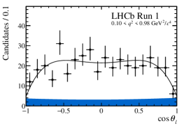
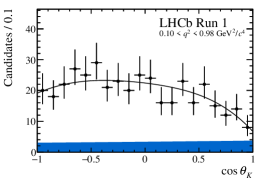
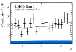
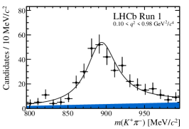
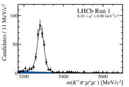
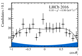
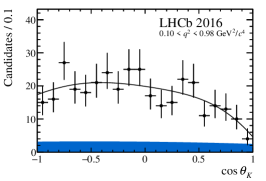
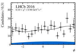
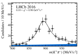
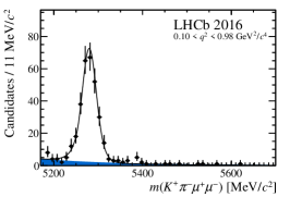
Figure 5: Projections of the fitted probability density function on the decay angles, $m({{K}^{+}}{{\pi}^{-}})$ and $m({{K}^{+}}{{\pi}^{-}}{\mu^{+}\mu^{-}})$ for the bin $0.10<q^{2}<0.98\text{\,Ge\kern-1.00006ptV}^{2}\!/c^{4}$. The blue shaded region indicates background.

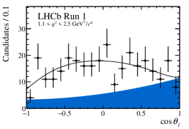
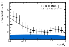
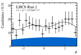
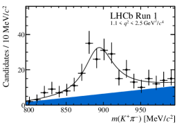
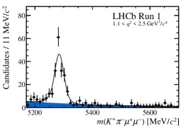
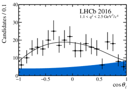
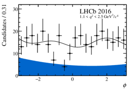
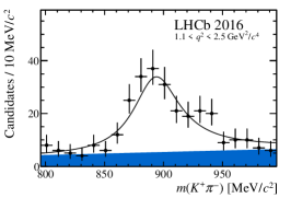
Figure 6: Projections of the fitted probability density function on the decay angles, $m({{K}^{+}}{{\pi}^{-}})$ and $m({{K}^{+}}{{\pi}^{-}}{\mu^{+}\mu^{-}})$ for the bin $1.1<q^{2}<2.5\text{\,Ge\kern-1.00006ptV}^{2}\!/c^{4}$. The blue shaded region indicates background.

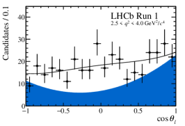
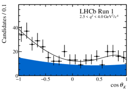
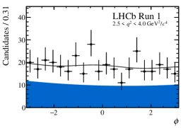
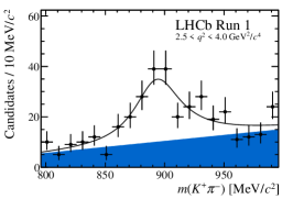
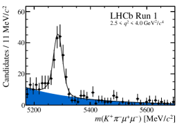
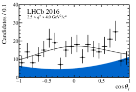
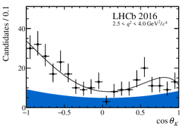
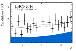
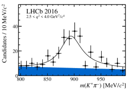
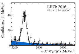
Figure 7: Projections of the fitted probability density function on the decay angles, $m({{K}^{+}}{{\pi}^{-}})$ and $m({{K}^{+}}{{\pi}^{-}}{\mu^{+}\mu^{-}})$ for the bin $2.5<q^{2}<4.0\text{\,Ge\kern-1.00006ptV}^{2}\!/c^{4}$. The blue shaded region indicates background.

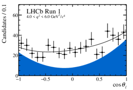
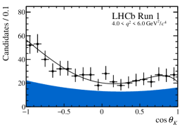
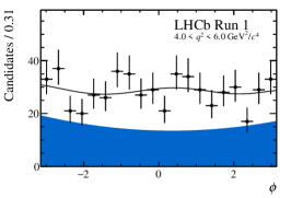
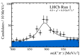
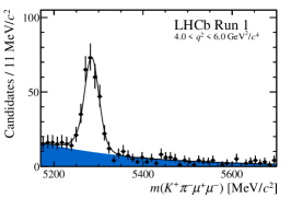
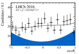
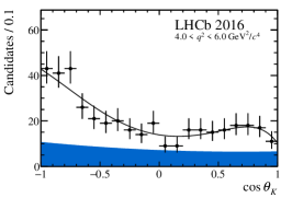
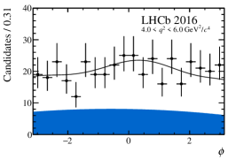
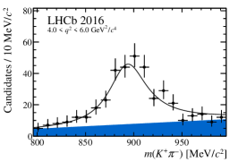
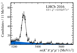
Figure 8: Projections of the fitted probability density function on the decay angles, $m({{K}^{+}}{{\pi}^{-}})$ and $m({{K}^{+}}{{\pi}^{-}}{\mu^{+}\mu^{-}})$ for the bin $4.0<q^{2}<6.0\text{\,Ge\kern-1.00006ptV}^{2}\!/c^{4}$. The blue shaded region indicates background.

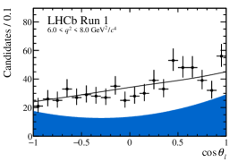
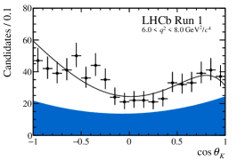
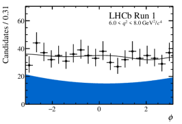
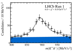
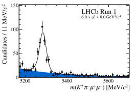
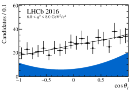
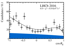
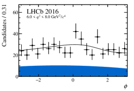
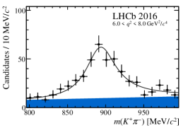
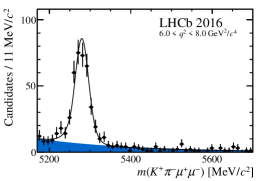
Figure 9: Projections of the fitted probability density function on the decay angles, $m({{K}^{+}}{{\pi}^{-}})$ and $m({{K}^{+}}{{\pi}^{-}}{\mu^{+}\mu^{-}})$ for the bin $6.0<q^{2}<8.0\text{\,Ge\kern-1.00006ptV}^{2}\!/c^{4}$. The blue shaded region indicates background.

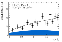
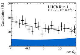
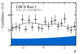
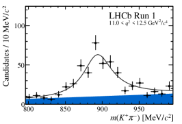
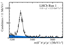
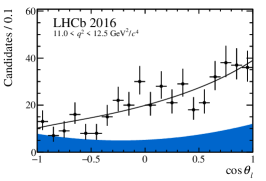
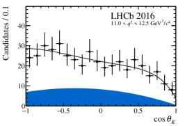
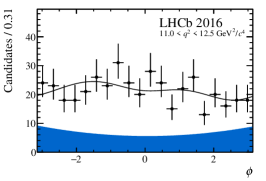
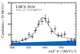
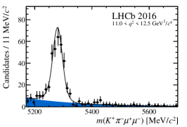
Figure 10: Projections of the fitted probability density function on the decay angles, $m({{K}^{+}}{{\pi}^{-}})$ and $m({{K}^{+}}{{\pi}^{-}}{\mu^{+}\mu^{-}})$ for the bin $11.0<q^{2}<12.5\text{\,Ge\kern-1.00006ptV}^{2}\!/c^{4}$. The blue shaded region indicates background.

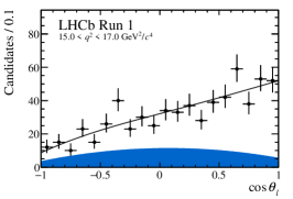
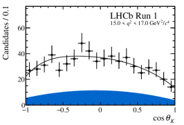
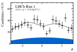
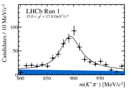
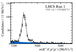
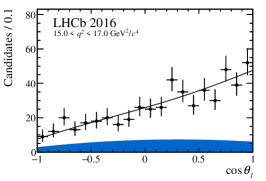
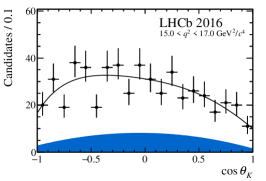
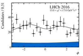
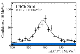
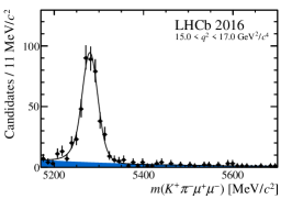
Figure 11: Projections of the fitted probability density function on the decay angles, $m({{K}^{+}}{{\pi}^{-}})$ and $m({{K}^{+}}{{\pi}^{-}}{\mu^{+}\mu^{-}})$ for the bin $15.0<q^{2}<17.0\text{\,Ge\kern-1.00006ptV}^{2}\!/c^{4}$. The blue shaded region indicates background.

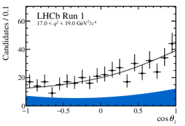
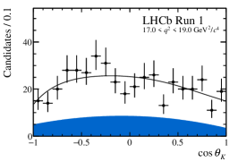
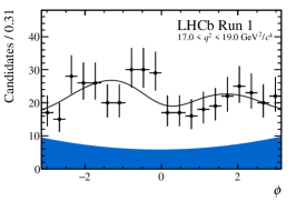
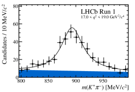
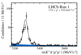
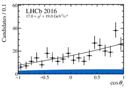
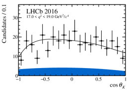
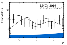
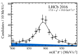
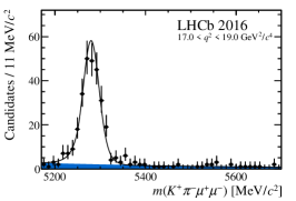
Figure 12: Projections of the fitted probability density function on the decay angles, $m({{K}^{+}}{{\pi}^{-}})$ and $m({{K}^{+}}{{\pi}^{-}}{\mu^{+}\mu^{-}})$ for the bin $17.0<q^{2}<19.0\text{\,Ge\kern-1.00006ptV}^{2}\!/c^{4}$. The blue shaded region indicates background.

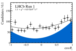
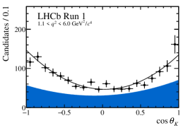
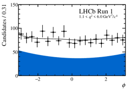
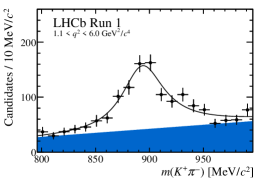
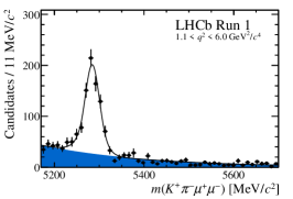
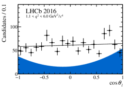
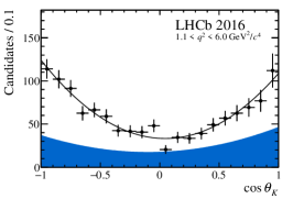
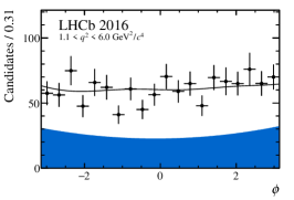
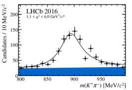
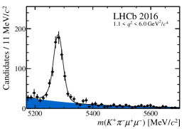
Figure 13: Projections of the fitted probability density function on the decay angles, $m({{K}^{+}}{{\pi}^{-}})$ and $m({{K}^{+}}{{\pi}^{-}}{\mu^{+}\mu^{-}})$ for the bin $1.1<q^{2}<6.0\text{\,Ge\kern-1.00006ptV}^{2}\!/c^{4}$. The blue shaded region indicates background.

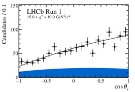
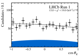
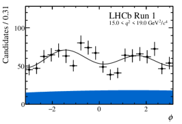
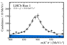
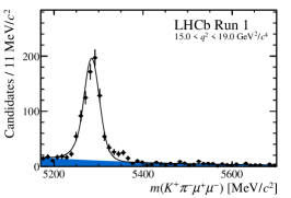
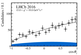
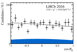
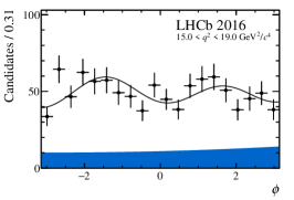
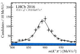
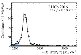
Figure 14: Projections of the fitted probability density function on the decay angles, $m({{K}^{+}}{{\pi}^{-}})$ and $m({{K}^{+}}{{\pi}^{-}}{\mu^{+}\mu^{-}})$ for the bin $15.0<q^{2}<19.0\text{\,Ge\kern-1.00006ptV}^{2}\!/c^{4}$. The blue shaded region indicates background.

LHCb collaboration

R. Aaij³¹, C. Abellán Beteta⁴⁹, T. Ackernley⁵⁹, B. Adeva⁴⁵, M. Adinolfi⁵³, H. Afsharnia⁹, C.A. Aidala⁸¹, S. Aiola²⁵, Z. Ajaltouni⁹, S. Akar⁶⁶, P. Albicocco²², J. Albrecht¹⁴, F. Alessio⁴⁷, M. Alexander⁵⁸, A. Alfonso Albero⁴⁴, G. Alkhazov³⁷, P. Alvarez Cartelle⁶⁰, A.A. Alves Jr⁴⁵, S. Amato², Y. Amhis¹¹, L. An²¹, L. Anderlini²¹, G. Andreassi⁴⁸, M. Andreotti²⁰, F. Archilli¹⁶, A. Artamonov⁴³, M. Artuso⁶⁷, K. Arzymatov⁴¹, E. Aslanides¹⁰, M. Atzeni⁴⁹, B. Audurier¹¹, S. Bachmann¹⁶, J.J. Back⁵⁵, S. Baker⁶⁰, V. Balagura^11,b, W. Baldini²⁰, A. Baranov⁴¹, R.J. Barlow⁶¹, S. Barsuk¹¹, W. Barter⁶⁰, M. Bartolini^23,47,h, F. Baryshnikov⁷⁸, J.M. Basels¹³, G. Bassi²⁸, V. Batozskaya³⁵, B. Batsukh⁶⁷, A. Battig¹⁴, A. Bay⁴⁸, M. Becker¹⁴, F. Bedeschi²⁸, I. Bediaga¹, A. Beiter⁶⁷, V. Belavin⁴¹, S. Belin²⁶, V. Bellee⁴⁸, K. Belous⁴³, I. Belyaev³⁸, G. Bencivenni²², E. Ben-Haim¹², S. Benson³¹, A. Berezhnoy³⁹, R. Bernet⁴⁹, D. Berninghoff¹⁶, H.C. Bernstein⁶⁷, C. Bertella⁴⁷, E. Bertholet¹², A. Bertolin²⁷, C. Betancourt⁴⁹, F. Betti^19,e, M.O. Bettler⁵⁴, Ia. Bezshyiko⁴⁹, S. Bhasin⁵³, J. Bhom³³, M.S. Bieker¹⁴, S. Bifani⁵², P. Billoir¹², A. Bizzeti^21,t, M. Bjørn⁶², M.P. Blago⁴⁷, T. Blake⁵⁵, F. Blanc⁴⁸, S. Blusk⁶⁷, D. Bobulska⁵⁸, V. Bocci³⁰, O. Boente Garcia⁴⁵, T. Boettcher⁶³, A. Boldyrev⁷⁹, A. Bondar^42,w, N. Bondar^37,47, S. Borghi⁶¹, M. Borisyak⁴¹, M. Borsato¹⁶, J.T. Borsuk³³, T.J.V. Bowcock⁵⁹, C. Bozzi²⁰, M.J. Bradley⁶⁰, S. Braun⁶⁵, A. Brea Rodriguez⁴⁵, M. Brodski⁴⁷, J. Brodzicka³³, A. Brossa Gonzalo⁵⁵, D. Brundu²⁶, E. Buchanan⁵³, A. Büchler-Germann⁴⁹, A. Buonaura⁴⁹, C. Burr⁴⁷, A. Bursche²⁶, A. Butkevich⁴⁰, J.S. Butter³¹, J. Buytaert⁴⁷, W. Byczynski⁴⁷, S. Cadeddu²⁶, H. Cai⁷², R. Calabrese^20,g, L. Calero Diaz²², S. Cali²², R. Calladine⁵², M. Calvi^24,i, M. Calvo Gomez^44,l, P. Camargo Magalhaes⁵³, A. Camboni^44,l, P. Campana²², D.H. Campora Perez³¹, A.F. Campoverde Quezada⁵, L. Capriotti^19,e, A. Carbone^19,e, G. Carboni²⁹, R. Cardinale^23,h, A. Cardini²⁶, I. Carli⁶, P. Carniti^24,i, K. Carvalho Akiba³¹, A. Casais Vidal⁴⁵, G. Casse⁵⁹, M. Cattaneo⁴⁷, G. Cavallero⁴⁷, S. Celani⁴⁸, R. Cenci^28,o, J. Cerasoli¹⁰, M.G. Chapman⁵³, M. Charles¹², Ph. Charpentier⁴⁷, G. Chatzikonstantinidis⁵², M. Chefdeville⁸, V. Chekalina⁴¹, C. Chen³, S. Chen²⁶, A. Chernov³³, S.-G. Chitic⁴⁷, V. Chobanova⁴⁵, S. Cholak⁴⁸, M. Chrzaszcz³³, A. Chubykin³⁷, V. Chulikov³⁷, P. Ciambrone²², M.F. Cicala⁵⁵, X. Cid Vidal⁴⁵, G. Ciezarek⁴⁷, F. Cindolo¹⁹, P.E.L. Clarke⁵⁷, M. Clemencic⁴⁷, H.V. Cliff⁵⁴, J. Closier⁴⁷, J.L. Cobbledick⁶¹, V. Coco⁴⁷, J.A.B. Coelho¹¹, J. Cogan¹⁰, E. Cogneras⁹, L. Cojocariu³⁶, P. Collins⁴⁷, T. Colombo⁴⁷, A. Contu²⁶, N. Cooke⁵², G. Coombs⁵⁸, S. Coquereau⁴⁴, G. Corti⁴⁷, C.M. Costa Sobral⁵⁵, B. Couturier⁴⁷, D.C. Craik⁶³, J. Crkovská⁶⁶, A. Crocombe⁵⁵, M. Cruz Torres^1,z, R. Currie⁵⁷, C.L. Da Silva⁶⁶, E. Dall’Occo¹⁴, J. Dalseno^45,53, C. D’Ambrosio⁴⁷, A. Danilina³⁸, P. d’Argent⁴⁷, A. Davis⁶¹, O. De Aguiar Francisco⁴⁷, K. De Bruyn⁴⁷, S. De Capua⁶¹, M. De Cian⁴⁸, J.M. De Miranda¹, L. De Paula², M. De Serio^18,d, P. De Simone²², J.A. de Vries⁷⁶, C.T. Dean⁶⁶, W. Dean⁸¹, D. Decamp⁸, L. Del Buono¹², B. Delaney⁵⁴, H.-P. Dembinski¹⁴, A. Dendek³⁴, V. Denysenko⁴⁹, D. Derkach⁷⁹, O. Deschamps⁹, F. Desse¹¹, F. Dettori^26,f, B. Dey⁷, A. Di Canto⁴⁷, P. Di Nezza²², S. Didenko⁷⁸, H. Dijkstra⁴⁷, V. Dobishuk⁵¹, F. Dordei²⁶, M. Dorigo^28,x, A.C. dos Reis¹, L. Douglas⁵⁸, A. Dovbnya⁵⁰, K. Dreimanis⁵⁹, M.W. Dudek³³, L. Dufour⁴⁷, P. Durante⁴⁷, J.M. Durham⁶⁶, D. Dutta⁶¹, M. Dziewiecki¹⁶, A. Dziurda³³, A. Dzyuba³⁷, S. Easo⁵⁶, U. Egede⁶⁹, V. Egorychev³⁸, S. Eidelman^42,w, S. Eisenhardt⁵⁷, S. Ek-In⁴⁸, L. Eklund⁵⁸, S. Ely⁶⁷, A. Ene³⁶, E. Epple⁶⁶, S. Escher¹³, J. Eschle⁴⁹, S. Esen³¹, T. Evans⁴⁷, A. Falabella¹⁹, J. Fan³, Y. Fan⁵, N. Farley⁵², S. Farry⁵⁹, D. Fazzini¹¹, P. Fedin³⁸, M. Féo⁴⁷, P. Fernandez Declara⁴⁷, A. Fernandez Prieto⁴⁵, F. Ferrari^19,e, L. Ferreira Lopes⁴⁸, F. Ferreira Rodrigues², S. Ferreres Sole³¹, M. Ferrillo⁴⁹, M. Ferro-Luzzi⁴⁷, S. Filippov⁴⁰, R.A. Fini¹⁸, M. Fiorini^20,g, M. Firlej³⁴, K.M. Fischer⁶², C. Fitzpatrick⁴⁷, T. Fiutowski³⁴, F. Fleuret^11,b, M. Fontana⁴⁷, F. Fontanelli^23,h, R. Forty⁴⁷, V. Franco Lima⁵⁹, M. Franco Sevilla⁶⁵, M. Frank⁴⁷, C. Frei⁴⁷, D.A. Friday⁵⁸, J. Fu^25,p, Q. Fuehring¹⁴, W. Funk⁴⁷, E. Gabriel⁵⁷, T. Gaintseva⁴¹, A. Gallas Torreira⁴⁵, D. Galli^19,e, S. Gallorini²⁷, S. Gambetta⁵⁷, Y. Gan³, M. Gandelman², P. Gandini²⁵, Y. Gao⁴, L.M. Garcia Martin⁴⁶, J. García Pardiñas⁴⁹, B. Garcia Plana⁴⁵, F.A. Garcia Rosales¹¹, L. Garrido⁴⁴, D. Gascon⁴⁴, C. Gaspar⁴⁷, D. Gerick¹⁶, E. Gersabeck⁶¹, M. Gersabeck⁶¹, T. Gershon⁵⁵, D. Gerstel¹⁰, Ph. Ghez⁸, V. Gibson⁵⁴, A. Gioventù⁴⁵, P. Gironella Gironell⁴⁴, L. Giubega³⁶, C. Giugliano²⁰, K. Gizdov⁵⁷, V.V. Gligorov¹², C. Göbel⁷⁰, D. Golubkov³⁸, A. Golutvin^60,78, A. Gomes^1,a, P. Gorbounov³⁸, I.V. Gorelov³⁹, C. Gotti^24,i, E. Govorkova³¹, J.P. Grabowski¹⁶, R. Graciani Diaz⁴⁴, T. Grammatico¹², L.A. Granado Cardoso⁴⁷, E. Graugés⁴⁴, E. Graverini⁴⁸, G. Graziani²¹, A. Grecu³⁶, R. Greim³¹, P. Griffith²⁰, L. Grillo⁶¹, L. Gruber⁴⁷, B.R. Gruberg Cazon⁶², C. Gu³, E. Gushchin⁴⁰, A. Guth¹³, Yu. Guz^43,47, T. Gys⁴⁷, P. A. Günther¹⁶, T. Hadavizadeh⁶², G. Haefeli⁴⁸, C. Haen⁴⁷, S.C. Haines⁵⁴, P.M. Hamilton⁶⁵, Q. Han⁷, X. Han¹⁶, T.H. Hancock⁶², S. Hansmann-Menzemer¹⁶, N. Harnew⁶², T. Harrison⁵⁹, R. Hart³¹, C. Hasse¹⁴, M. Hatch⁴⁷, J. He⁵, M. Hecker⁶⁰, K. Heijhoff³¹, K. Heinicke¹⁴, A.M. Hennequin⁴⁷, K. Hennessy⁵⁹, L. Henry^25,46, J. Heuel¹³, A. Hicheur⁶⁸, D. Hill⁶², M. Hilton⁶¹, P.H. Hopchev⁴⁸, J. Hu¹⁶, J. Hu⁷¹, W. Hu⁷, W. Huang⁵, W. Hulsbergen³¹, T. Humair⁶⁰, R.J. Hunter⁵⁵, M. Hushchyn⁷⁹, D. Hutchcroft⁵⁹, D. Hynds³¹, P. Ibis¹⁴, M. Idzik³⁴, P. Ilten⁵², A. Inglessi³⁷, K. Ivshin³⁷, R. Jacobsson⁴⁷, S. Jakobsen⁴⁷, E. Jans³¹, B.K. Jashal⁴⁶, A. Jawahery⁶⁵, V. Jevtic¹⁴, F. Jiang³, M. John⁶², D. Johnson⁴⁷, C.R. Jones⁵⁴, B. Jost⁴⁷, N. Jurik⁶², S. Kandybei⁵⁰, M. Karacson⁴⁷, J.M. Kariuki⁵³, N. Kazeev⁷⁹, M. Kecke¹⁶, F. Keizer^54,47, M. Kelsey⁶⁷, M. Kenzie⁵⁵, T. Ketel³², B. Khanji⁴⁷, A. Kharisova⁸⁰, K.E. Kim⁶⁷, T. Kirn¹³, V.S. Kirsebom⁴⁸, S. Klaver²², K. Klimaszewski³⁵, S. Koliiev⁵¹, A. Kondybayeva⁷⁸, A. Konoplyannikov³⁸, P. Kopciewicz³⁴, R. Kopecna¹⁶, P. Koppenburg³¹, M. Korolev³⁹, I. Kostiuk^31,51, O. Kot⁵¹, S. Kotriakhova³⁷, L. Kravchuk⁴⁰, R.D. Krawczyk⁴⁷, M. Kreps⁵⁵, F. Kress⁶⁰, S. Kretzschmar¹³, P. Krokovny^42,w, W. Krupa³⁴, W. Krzemien³⁵, W. Kucewicz^33,k, M. Kucharczyk³³, V. Kudryavtsev^42,w, H.S. Kuindersma³¹, G.J. Kunde⁶⁶, T. Kvaratskheliya³⁸, D. Lacarrere⁴⁷, G. Lafferty⁶¹, A. Lai²⁶, D. Lancierini⁴⁹, J.J. Lane⁶¹, G. Lanfranchi²², C. Langenbruch¹³, O. Lantwin⁴⁹, T. Latham⁵⁵, F. Lazzari^28,u, R. Le Gac¹⁰, S.H. Lee⁸¹, R. Lefèvre⁹, A. Leflat^39,47, O. Leroy¹⁰, T. Lesiak³³, B. Leverington¹⁶, H. Li⁷¹, L. Li⁶², X. Li⁶⁶, Y. Li⁶, Z. Li⁶⁷, X. Liang⁶⁷, T. Lin⁶⁰, R. Lindner⁴⁷, V. Lisovskyi¹⁴, G. Liu⁷¹, X. Liu³, D. Loh⁵⁵, A. Loi²⁶, J. Lomba Castro⁴⁵, I. Longstaff⁵⁸, J.H. Lopes², G. Loustau⁴⁹, G.H. Lovell⁵⁴, Y. Lu⁶, D. Lucchesi^27,n, M. Lucio Martinez³¹, Y. Luo³, A. Lupato²⁷, E. Luppi^20,g, O. Lupton⁵⁵, A. Lusiani^28,s, X. Lyu⁵, S. Maccolini^19,e, F. Machefert¹¹, F. Maciuc³⁶, V. Macko⁴⁸, P. Mackowiak¹⁴, S. Maddrell-Mander⁵³, L.R. Madhan Mohan⁵³, O. Maev³⁷, A. Maevskiy⁷⁹, D. Maisuzenko³⁷, M.W. Majewski³⁴, S. Malde⁶², B. Malecki⁴⁷, A. Malinin⁷⁷, T. Maltsev^42,w, H. Malygina¹⁶, G. Manca^26,f, G. Mancinelli¹⁰, R. Manera Escalero⁴⁴, D. Manuzzi^19,e, D. Marangotto²⁵, J. Maratas^9,v, J.F. Marchand⁸, U. Marconi¹⁹, S. Mariani^21,21,47, C. Marin Benito¹¹, M. Marinangeli⁴⁸, P. Marino⁴⁸, J. Marks¹⁶, P.J. Marshall⁵⁹, G. Martellotti³⁰, L. Martinazzoli⁴⁷, M. Martinelli^24,i, D. Martinez Santos⁴⁵, F. Martinez Vidal⁴⁶, A. Massafferri¹, M. Materok¹³, R. Matev⁴⁷, A. Mathad⁴⁹, Z. Mathe⁴⁷, V. Matiunin³⁸, C. Matteuzzi²⁴, K.R. Mattioli⁸¹, A. Mauri⁴⁹, E. Maurice^11,b, M. McCann⁶⁰, L. Mcconnell¹⁷, A. McNab⁶¹, R. McNulty¹⁷, J.V. Mead⁵⁹, B. Meadows⁶⁴, C. Meaux¹⁰, G. Meier¹⁴, N. Meinert⁷⁴, D. Melnychuk³⁵, S. Meloni^24,i, M. Merk³¹, A. Merli²⁵, M. Mikhasenko⁴⁷, D.A. Milanes⁷³, E. Millard⁵⁵, M.-N. Minard⁸, O. Mineev³⁸, L. Minzoni²⁰, S.E. Mitchell⁵⁷, B. Mitreska⁶¹, D.S. Mitzel⁴⁷, A. Mödden¹⁴, A. Mogini¹², R.D. Moise⁶⁰, T. Mombächer¹⁴, I.A. Monroy⁷³, S. Monteil⁹, M. Morandin²⁷, G. Morello²², M.J. Morello^28,s, J. Moron³⁴, A.B. Morris¹⁰, A.G. Morris⁵⁵, R. Mountain⁶⁷, H. Mu³, F. Muheim⁵⁷, M. Mukherjee⁷, M. Mulder⁴⁷, D. Müller⁴⁷, K. Müller⁴⁹, C.H. Murphy⁶², D. Murray⁶¹, P. Muzzetto²⁶, P. Naik⁵³, T. Nakada⁴⁸, R. Nandakumar⁵⁶, T. Nanut⁴⁸, I. Nasteva², M. Needham⁵⁷, N. Neri^25,p, S. Neubert¹⁶, N. Neufeld⁴⁷, R. Newcombe⁶⁰, T.D. Nguyen⁴⁸, C. Nguyen-Mau^48,m, E.M. Niel¹¹, S. Nieswand¹³, N. Nikitin³⁹, N.S. Nolte⁴⁷, C. Nunez⁸¹, A. Oblakowska-Mucha³⁴, V. Obraztsov⁴³, S. Ogilvy⁵⁸, D.P. O’Hanlon⁵³, R. Oldeman^26,f, C.J.G. Onderwater⁷⁵, J. D. Osborn⁸¹, A. Ossowska³³, J.M. Otalora Goicochea², T. Ovsiannikova³⁸, P. Owen⁴⁹, A. Oyanguren⁴⁶, P.R. Pais⁴⁸, T. Pajero^28,28,47,s, A. Palano¹⁸, M. Palutan²², G. Panshin⁸⁰, A. Papanestis⁵⁶, M. Pappagallo⁵⁷, L.L. Pappalardo²⁰, C. Pappenheimer⁶⁴, W. Parker⁶⁵, C. Parkes⁶¹, G. Passaleva^21,47, A. Pastore¹⁸, M. Patel⁶⁰, C. Patrignani^19,e, A. Pearce⁴⁷, A. Pellegrino³¹, M. Pepe Altarelli⁴⁷, S. Perazzini¹⁹, D. Pereima³⁸, P. Perret⁹, L. Pescatore⁴⁸, K. Petridis⁵³, A. Petrolini^23,h, A. Petrov⁷⁷, S. Petrucci⁵⁷, M. Petruzzo^25,p, B. Pietrzyk⁸, G. Pietrzyk⁴⁸, M. Pili⁶², D. Pinci³⁰, J. Pinzino⁴⁷, F. Pisani¹⁹, A. Piucci¹⁶, V. Placinta³⁶, S. Playfer⁵⁷, J. Plews⁵², M. Plo Casasus⁴⁵, F. Polci¹², M. Poli Lener²², M. Poliakova⁶⁷, A. Poluektov¹⁰, N. Polukhina^78,c, I. Polyakov⁶⁷, E. Polycarpo², G.J. Pomery⁵³, S. Ponce⁴⁷, A. Popov⁴³, D. Popov⁵², S. Poslavskii⁴³, K. Prasanth³³, L. Promberger⁴⁷, C. Prouve⁴⁵, V. Pugatch⁵¹, A. Puig Navarro⁴⁹, H. Pullen⁶², G. Punzi^28,o, W. Qian⁵, J. Qin⁵, R. Quagliani¹², B. Quintana⁸, N.V. Raab¹⁷, R.I. Rabadan Trejo¹⁰, B. Rachwal³⁴, J.H. Rademacker⁵³, M. Rama²⁸, M. Ramos Pernas⁴⁵, M.S. Rangel², F. Ratnikov^41,79, G. Raven³², M. Reboud⁸, F. Redi⁴⁸, F. Reiss¹², C. Remon Alepuz⁴⁶, Z. Ren³, V. Renaudin⁶², S. Ricciardi⁵⁶, D.S. Richards⁵⁶, S. Richards⁵³, K. Rinnert⁵⁹, P. Robbe¹¹, A. Robert¹², A.B. Rodrigues⁴⁸, E. Rodrigues⁵⁹, J.A. Rodriguez Lopez⁷³, M. Roehrken⁴⁷, A. Rollings⁶², V. Romanovskiy⁴³, M. Romero Lamas⁴⁵, A. Romero Vidal⁴⁵, J.D. Roth⁸¹, M. Rotondo²², M.S. Rudolph⁶⁷, T. Ruf⁴⁷, J. Ruiz Vidal⁴⁶, A. Ryzhikov⁷⁹, J. Ryzka³⁴, J.J. Saborido Silva⁴⁵, N. Sagidova³⁷, N. Sahoo⁵⁵, B. Saitta^26,f, C. Sanchez Gras³¹, C. Sanchez Mayordomo⁴⁶, R. Santacesaria³⁰, C. Santamarina Rios⁴⁵, M. Santimaria²², E. Santovetti^29,j, G. Sarpis⁶¹, M. Sarpis¹⁶, A. Sarti³⁰, C. Satriano^30,r, A. Satta²⁹, M. Saur⁵, D. Savrina^38,39, L.G. Scantlebury Smead⁶², S. Schael¹³, M. Schellenberg¹⁴, M. Schiller⁵⁸, H. Schindler⁴⁷, M. Schmelling¹⁵, T. Schmelzer¹⁴, B. Schmidt⁴⁷, O. Schneider⁴⁸, A. Schopper⁴⁷, H.F. Schreiner⁶⁴, M. Schubiger³¹, S. Schulte⁴⁸, M.H. Schune¹¹, R. Schwemmer⁴⁷, B. Sciascia²², A. Sciubba²², S. Sellam⁶⁸, A. Semennikov³⁸, A. Sergi^52,47, N. Serra⁴⁹, J. Serrano¹⁰, L. Sestini²⁷, A. Seuthe¹⁴, P. Seyfert⁴⁷, D.M. Shangase⁸¹, M. Shapkin⁴³, L. Shchutska⁴⁸, T. Shears⁵⁹, L. Shekhtman^42,w, V. Shevchenko⁷⁷, E. Shmanin⁷⁸, J.D. Shupperd⁶⁷, B.G. Siddi²⁰, R. Silva Coutinho⁴⁹, L. Silva de Oliveira², G. Simi^27,n, S. Simone^18,d, I. Skiba²⁰, N. Skidmore¹⁶, T. Skwarnicki⁶⁷, M.W. Slater⁵², J.G. Smeaton⁵⁴, A. Smetkina³⁸, E. Smith¹³, I.T. Smith⁵⁷, M. Smith⁶⁰, A. Snoch³¹, M. Soares¹⁹, L. Soares Lavra⁹, M.D. Sokoloff⁶⁴, F.J.P. Soler⁵⁸, B. Souza De Paula², B. Spaan¹⁴, E. Spadaro Norella^25,p, P. Spradlin⁵⁸, F. Stagni⁴⁷, M. Stahl⁶⁴, S. Stahl⁴⁷, P. Stefko⁴⁸, O. Steinkamp^49,78, S. Stemmle¹⁶, O. Stenyakin⁴³, M. Stepanova³⁷, H. Stevens¹⁴, S. Stone⁶⁷, S. Stracka²⁸, M.E. Stramaglia⁴⁸, M. Straticiuc³⁶, S. Strokov⁸⁰, J. Sun²⁶, L. Sun⁷², Y. Sun⁶⁵, P. Svihra⁶¹, K. Swientek³⁴, A. Szabelski³⁵, T. Szumlak³⁴, M. Szymanski⁴⁷, S. Taneja⁶¹, Z. Tang³, T. Tekampe¹⁴, F. Teubert⁴⁷, E. Thomas⁴⁷, K.A. Thomson⁵⁹, M.J. Tilley⁶⁰, V. Tisserand⁹, S. T’Jampens⁸, M. Tobin⁶, S. Tolk⁴⁷, L. Tomassetti^20,g, D. Torres Machado¹, D.Y. Tou¹², E. Tournefier⁸, M. Traill⁵⁸, M.T. Tran⁴⁸, E. Trifonova⁷⁸, C. Trippl⁴⁸, A. Tsaregorodtsev¹⁰, G. Tuci^28,o, A. Tully⁴⁸, N. Tuning³¹, A. Ukleja³⁵, A. Usachov³¹, A. Ustyuzhanin^41,79, U. Uwer¹⁶, A. Vagner⁸⁰, V. Vagnoni¹⁹, A. Valassi⁴⁷, G. Valenti¹⁹, M. van Beuzekom³¹, H. Van Hecke⁶⁶, E. van Herwijnen⁴⁷, C.B. Van Hulse¹⁷, M. van Veghel⁷⁵, R. Vazquez Gomez⁴⁴, P. Vazquez Regueiro⁴⁵, C. Vázquez Sierra³¹, S. Vecchi²⁰, J.J. Velthuis⁵³, M. Veltri^21,q, A. Venkateswaran⁶⁷, M. Veronesi³¹, M. Vesterinen⁵⁵, J.V. Viana Barbosa⁴⁷, D. Vieira⁶⁴, M. Vieites Diaz⁴⁸, H. Viemann⁷⁴, X. Vilasis-Cardona^44,l, G. Vitali²⁸, A. Vitkovskiy³¹, A. Vollhardt⁴⁹, D. Vom Bruch¹², A. Vorobyev³⁷, V. Vorobyev^42,w, N. Voropaev³⁷, R. Waldi⁷⁴, J. Walsh²⁸, J. Wang³, J. Wang⁷², J. Wang⁶, M. Wang³, Y. Wang⁷, Z. Wang⁴⁹, D.R. Ward⁵⁴, H.M. Wark⁵⁹, N.K. Watson⁵², D. Websdale⁶⁰, A. Weiden⁴⁹, C. Weisser⁶³, B.D.C. Westhenry⁵³, D.J. White⁶¹, M. Whitehead¹³, D. Wiedner¹⁴, G. Wilkinson⁶², M. Wilkinson⁶⁷, I. Williams⁵⁴, M. Williams⁶³, M.R.J. Williams⁶¹, T. Williams⁵², F.F. Wilson⁵⁶, W. Wislicki³⁵, M. Witek³³, L. Witola¹⁶, G. Wormser¹¹, S.A. Wotton⁵⁴, H. Wu⁶⁷, K. Wyllie⁴⁷, Z. Xiang⁵, D. Xiao⁷, Y. Xie⁷, H. Xing⁷¹, A. Xu⁴, J. Xu⁵, L. Xu³, M. Xu⁷, Q. Xu⁵, Z. Xu⁴, Z. Yang³, Z. Yang⁶⁵, Y. Yao⁶⁷, L.E. Yeomans⁵⁹, H. Yin⁷, J. Yu⁷, X. Yuan⁶⁷, O. Yushchenko⁴³, K.A. Zarebski⁵², M. Zavertyaev^15,c, M. Zdybal³³, M. Zeng³, D. Zhang⁷, L. Zhang³, S. Zhang⁴, W.C. Zhang^3,y, Y. Zhang⁴⁷, A. Zhelezov¹⁶, Y. Zheng⁵, X. Zhou⁵, Y. Zhou⁵, X. Zhu³, V. Zhukov^13,39, J.B. Zonneveld⁵⁷, S. Zucchelli^19,e.

¹Centro Brasileiro de Pesquisas Físicas (CBPF), Rio de Janeiro, Brazil
²Universidade Federal do Rio de Janeiro (UFRJ), Rio de Janeiro, Brazil
³Center for High Energy Physics, Tsinghua University, Beijing, China
⁴School of Physics State Key Laboratory of Nuclear Physics and Technology, Peking University, Beijing, China
⁵University of Chinese Academy of Sciences, Beijing, China
⁶Institute Of High Energy Physics (IHEP), Beijing, China
⁷Institute of Particle Physics, Central China Normal University, Wuhan, Hubei, China
⁸Univ. Grenoble Alpes, Univ. Savoie Mont Blanc, CNRS, IN2P3-LAPP, Annecy, France
⁹Université Clermont Auvergne, CNRS/IN2P3, LPC, Clermont-Ferrand, France
¹⁰Aix Marseille Univ, CNRS/IN2P3, CPPM, Marseille, France
¹¹Université Paris-Saclay, CNRS/IN2P3, IJCLab, 91405 Orsay, France , Orsay, France
¹²LPNHE, Sorbonne Université, Paris Diderot Sorbonne Paris Cité, CNRS/IN2P3, Paris, France
¹³I. Physikalisches Institut, RWTH Aachen University, Aachen, Germany
¹⁴Fakultät Physik, Technische Universität Dortmund, Dortmund, Germany
¹⁵Max-Planck-Institut für Kernphysik (MPIK), Heidelberg, Germany
¹⁶Physikalisches Institut, Ruprecht-Karls-Universität Heidelberg, Heidelberg, Germany
¹⁷School of Physics, University College Dublin, Dublin, Ireland
¹⁸INFN Sezione di Bari, Bari, Italy
¹⁹INFN Sezione di Bologna, Bologna, Italy
²⁰INFN Sezione di Ferrara, Ferrara, Italy
²¹INFN Sezione di Firenze, Firenze, Italy
²²INFN Laboratori Nazionali di Frascati, Frascati, Italy
²³INFN Sezione di Genova, Genova, Italy
²⁴INFN Sezione di Milano-Bicocca, Milano, Italy
²⁵INFN Sezione di Milano, Milano, Italy
²⁶INFN Sezione di Cagliari, Monserrato, Italy
²⁷INFN Sezione di Padova, Padova, Italy
²⁸INFN Sezione di Pisa, Pisa, Italy
²⁹INFN Sezione di Roma Tor Vergata, Roma, Italy
³⁰INFN Sezione di Roma La Sapienza, Roma, Italy
³¹Nikhef National Institute for Subatomic Physics, Amsterdam, Netherlands
³²Nikhef National Institute for Subatomic Physics and VU University Amsterdam, Amsterdam, Netherlands
³³Henryk Niewodniczanski Institute of Nuclear Physics Polish Academy of Sciences, Kraków, Poland
³⁴AGH - University of Science and Technology, Faculty of Physics and Applied Computer Science, Kraków, Poland
³⁵National Center for Nuclear Research (NCBJ), Warsaw, Poland
³⁶Horia Hulubei National Institute of Physics and Nuclear Engineering, Bucharest-Magurele, Romania
³⁷Petersburg Nuclear Physics Institute NRC Kurchatov Institute (PNPI NRC KI), Gatchina, Russia
³⁸Institute of Theoretical and Experimental Physics NRC Kurchatov Institute (ITEP NRC KI), Moscow, Russia, Moscow, Russia
³⁹Institute of Nuclear Physics, Moscow State University (SINP MSU), Moscow, Russia
⁴⁰Institute for Nuclear Research of the Russian Academy of Sciences (INR RAS), Moscow, Russia
⁴¹Yandex School of Data Analysis, Moscow, Russia
⁴²Budker Institute of Nuclear Physics (SB RAS), Novosibirsk, Russia
⁴³Institute for High Energy Physics NRC Kurchatov Institute (IHEP NRC KI), Protvino, Russia, Protvino, Russia
⁴⁴ICCUB, Universitat de Barcelona, Barcelona, Spain
⁴⁵Instituto Galego de Física de Altas Enerxías (IGFAE), Universidade de Santiago de Compostela, Santiago de Compostela, Spain
⁴⁶Instituto de Fisica Corpuscular, Centro Mixto Universidad de Valencia - CSIC, Valencia, Spain
⁴⁷European Organization for Nuclear Research (CERN), Geneva, Switzerland
⁴⁸Institute of Physics, Ecole Polytechnique Fédérale de Lausanne (EPFL), Lausanne, Switzerland
⁴⁹Physik-Institut, Universität Zürich, Zürich, Switzerland
⁵⁰NSC Kharkiv Institute of Physics and Technology (NSC KIPT), Kharkiv, Ukraine
⁵¹Institute for Nuclear Research of the National Academy of Sciences (KINR), Kyiv, Ukraine
⁵²University of Birmingham, Birmingham, United Kingdom
⁵³H.H. Wills Physics Laboratory, University of Bristol, Bristol, United Kingdom
⁵⁴Cavendish Laboratory, University of Cambridge, Cambridge, United Kingdom
⁵⁵Department of Physics, University of Warwick, Coventry, United Kingdom
⁵⁶STFC Rutherford Appleton Laboratory, Didcot, United Kingdom
⁵⁷School of Physics and Astronomy, University of Edinburgh, Edinburgh, United Kingdom
⁵⁸School of Physics and Astronomy, University of Glasgow, Glasgow, United Kingdom
⁵⁹Oliver Lodge Laboratory, University of Liverpool, Liverpool, United Kingdom
⁶⁰Imperial College London, London, United Kingdom
⁶¹Department of Physics and Astronomy, University of Manchester, Manchester, United Kingdom
⁶²Department of Physics, University of Oxford, Oxford, United Kingdom
⁶³Massachusetts Institute of Technology, Cambridge, MA, United States
⁶⁴University of Cincinnati, Cincinnati, OH, United States
⁶⁵University of Maryland, College Park, MD, United States
⁶⁶Los Alamos National Laboratory (LANL), Los Alamos, United States
⁶⁷Syracuse University, Syracuse, NY, United States
⁶⁸Laboratory of Mathematical and Subatomic Physics , Constantine, Algeria, associated to ^2
69School of Physics and Astronomy, Monash University, Melbourne, Australia, associated to ^55
70Pontifícia Universidade Católica do Rio de Janeiro (PUC-Rio), Rio de Janeiro, Brazil, associated to ^2
71Guangdong Provencial Key Laboratory of Nuclear Science, Institute of Quantum Matter, South China Normal University, Guangzhou, China, associated to ^3
72School of Physics and Technology, Wuhan University, Wuhan, China, associated to ^3
73Departamento de Fisica , Universidad Nacional de Colombia, Bogota, Colombia, associated to ^12
74Institut für Physik, Universität Rostock, Rostock, Germany, associated to ^16
75Van Swinderen Institute, University of Groningen, Groningen, Netherlands, associated to ^31
76Universiteit Maastricht, Maastricht, Netherlands, associated to ^31
77National Research Centre Kurchatov Institute, Moscow, Russia, associated to ^38
78National University of Science and Technology “MISIS”, Moscow, Russia, associated to ^38
79National Research University Higher School of Economics, Moscow, Russia, associated to ^41
80National Research Tomsk Polytechnic University, Tomsk, Russia, associated to ^38
81University of Michigan, Ann Arbor, United States, associated to <sup>67

a</sup>Universidade Federal do Triângulo Mineiro (UFTM), Uberaba-MG, Brazil
^bLaboratoire Leprince-Ringuet, Palaiseau, France
^cP.N. Lebedev Physical Institute, Russian Academy of Science (LPI RAS), Moscow, Russia
^dUniversità di Bari, Bari, Italy
^eUniversità di Bologna, Bologna, Italy
^fUniversità di Cagliari, Cagliari, Italy
^gUniversità di Ferrara, Ferrara, Italy
^hUniversità di Genova, Genova, Italy
ⁱUniversità di Milano Bicocca, Milano, Italy
^jUniversità di Roma Tor Vergata, Roma, Italy
^kAGH - University of Science and Technology, Faculty of Computer Science, Electronics and Telecommunications, Kraków, Poland
^lDS4DS, La Salle, Universitat Ramon Llull, Barcelona, Spain
^mHanoi University of Science, Hanoi, Vietnam
ⁿUniversità di Padova, Padova, Italy
^oUniversità di Pisa, Pisa, Italy
^pUniversità degli Studi di Milano, Milano, Italy
^qUniversità di Urbino, Urbino, Italy
^rUniversità della Basilicata, Potenza, Italy
^sScuola Normale Superiore, Pisa, Italy
^tUniversità di Modena e Reggio Emilia, Modena, Italy
^uUniversità di Siena, Siena, Italy
^vMSU - Iligan Institute of Technology (MSU-IIT), Iligan, Philippines
^wNovosibirsk State University, Novosibirsk, Russia
^xINFN Sezione di Trieste, Trieste, Italy
^ySchool of Physics and Information Technology, Shaanxi Normal University (SNNU), Xi’an, China
^zUniversidad Nacional Autonoma de Honduras, Tegucigalpa, Honduras

References

- [1] LHCb collaboration, R. Aaij et al., Angular analysis of the decay using of integrated luminosity, JHEP 02 (2016) 104, arXiv:1512.04442
- [2] CMS collaboration, A. M. Sirunyan et al., Measurement of angular parameters from the decay in proton-proton collisions at 8 TeV, Phys. Lett. B781 (2018) 517, arXiv:1710.02846
- [3] ATLAS collaboration, M. Aaboud et al., Angular analysis of decays in collisions at TeV with the ATLAS detector, JHEP 10 (2018) 047, arXiv:1805.04000
- [4] Belle collaboration, S. Wehle et al., Lepton-flavor-dependent angular analysis of , Phys. Rev. Lett. 118 (2017) 111801, arXiv:1612.05014
- [5] BaBar collaboration, B. Aubert et al., Measurements of branching fractions, rate asymmetries, and angular distributions in the rare decays and , Phys. Rev. D73 (2006) 092001, arXiv:hep-ex/0604007
- [6] CDF collaboration, T. Aaltonen et al., Measurements of the angular distributions in the decays at CDF, Phys. Rev. Lett. 108 (2012) 081807, arXiv:1108.0695
- [7] LHCb collaboration, R. Aaij et al., Angular moments of the decay at low hadronic recoil, JHEP 09 (2018) 146, arXiv:1808.00264
- [8] LHCb collaboration, R. Aaij et al., Angular analysis and differential branching fraction of the decay , JHEP 09 (2015) 179, arXiv:1506.08777
- [9] LHCb collaboration, R. Aaij et al., Measurements of the S-wave fraction in decays and the differential branching fraction, JHEP 11 (2016) 047, Erratum ibid. 04 (2017) 142, arXiv:1606.04731
- [10] LHCb collaboration, R. Aaij et al., Differential branching fraction and angular analysis of decays, JHEP 06 (2015) 115, Erratum ibid. 09 (2018) 145, arXiv:1503.07138
- [11] LHCb collaboration, R. Aaij et al., Differential branching fractions and isospin asymmetries of decays, JHEP 06 (2014) 133, arXiv:1403.8044
- [12] LHCb collaboration, R. Aaij et al., Search for lepton-universality violation in decays, Phys. Rev. Lett. 122 (2019) 191801, arXiv:1903.09252
- [13] Belle collaboration, A. Abdesselam et al., Test of lepton flavor universality in decays, arXiv:1908.01848
- [14] BaBar collaboration, J. P. Lees et al., Measurement of branching fractions and rate asymmetries in the rare decays , Phys. Rev. D86 (2012) 032012, arXiv:1204.3933
- [15] LHCb collaboration, R. Aaij et al., Test of lepton universality with decays, JHEP 08 (2017) 055, arXiv:1705.05802
- [16] Belle collaboration, A. Abdesselam et al., Test of lepton flavor universality in decays at Belle, arXiv:1904.02440
- [17] M. Algueró et al., Emerging patterns of new physics with and without Lepton flavour universal contributions, Eur. Phys. J. C79 (2019) 714, arXiv:1903.09578
- [18] J. Aebischer et al., -decay discrepancies after Moriond 2019, arXiv:1903.10434
- [19] A. Arbey et al., Update on the anomalies, Phys. Rev. D100 (2019) 015045, arXiv:1904.08399
- [20] M. Ciuchini et al., New physics in confronts new data on lepton universality, Eur. Phys. J. C79 (2019) 719, arXiv:1903.09632
- [21] K. Kowalska, D. Kumar, and E. M. Sessolo, Implications for new physics in transitions after recent measurements by Belle and LHCb, Eur. Phys. J. C79 (2019) 840, arXiv:1903.10932
- [22] A. K. Alok, A. Dighe, S. Gangal, and D. Kumar, Continuing search for new physics in decays: Two operators at a time, JHEP 06 (2019) 089, arXiv:1903.09617
- [23] W. Altmannshofer, S. Gori, M. Pospelov, and I. Yavin, Quark flavor transitions in models, Phys. Rev. D89 (2014) 095033, arXiv:1403.1269
- [24] A. Crivellin, G. D’Ambrosio, and J. Heeck, Explaining , and in a two-Higgs-doublet model with gauged , Phys. Rev. Lett. 114 (2015) 151801, arXiv:1501.00993
- [25] A. Celis, J. Fuentes-Martín, M. Jung, and H. Serôdio, Family nonuniversal models with protected flavor-changing interactions, Phys. Rev. D92 (2015) 015007, arXiv:1505.03079
- [26] A. Falkowski, M. Nardecchia, and R. Ziegler, Lepton flavor non-universality in -meson decays from a flavor model, JHEP 11 (2015) 173, arXiv:1509.01249
- [27] G. Hiller and M. Schmaltz, and future physics beyond the standard model opportunities, Phys. Rev. D90 (2014) 054014, arXiv:1408.1627
- [28] B. Gripaios, M. Nardecchia, and S. A. Renner, Composite leptoquarks and anomalies in -meson decays, JHEP 05 (2015) 006, arXiv:1412.1791
- [29] I. de Medeiros Varzielas and G. Hiller, Clues for flavor from rare lepton and quark decays, JHEP 06 (2015) 072, arXiv:1503.01084
- [30] R. Barbieri, C. W. Murphy, and F. Senia, -decay anomalies in a composite leptoquark model, Eur. Phys. J. C77 (2017) 8, arXiv:1611.04930
- [31] J.-H. Sheng, R.-M. Wang, and Y.-D. Yang, Scalar leptoquark effects in the lepton flavor violating exclusive Decays, Int. J. Theor. Phys. 58 (2019) 480, arXiv:1805.05059
- [32] G. Hiller, D. Loose, and I. Nis̆andz̆ić, Flavorful leptoquarks at hadron colliders, Phys. Rev. D97 (2018) 075004, arXiv:1801.09399
- [33] A. Crivellin, D. Müller, and T. Ota, Simultaneous explanation of R() and : the last scalar leptoquarks standing, JHEP 09 (2017) 040, arXiv:1703.09226
- [34] F. Sala and D. M. Straub, A new light particle in decays?, Phys. Lett. B774 (2017) 205–209
- [35] P. Ko, Y. Omura, Y. Shigekami, and C. Yu, LHCb anomaly and physics in flavored models with flavored Higgs doublets, Phys. Rev. D95 (2017) 115040
- [36] S. Jäger and J. Martin Camalich, Reassessing the discovery potential of the decays in the large-recoil region: SM challenges and BSM opportunities, Phys. Rev. D93 (2016) 014028, arXiv:1412.3183
- [37] J. Lyon and R. Zwicky, Resonances gone topsy turvy - the charm of QCD or new physics in ?, arXiv:1406.0566
- [38] M. Ciuchini et al., decays at large recoil in the Standard Model: a theoretical reappraisal, JHEP 06 (2016) 116, arXiv:1512.07157
- [39] C. Bobeth, M. Chrzaszcz, D. van Dyk, and J. Virto, Long-distance effects in from analyticity, Eur. Phys. J. C78 (2018) 451, arXiv:1707.07305
- [40] F. Beaujean, C. Bobeth, and D. van Dyk, Comprehensive Bayesian analysis of rare (semi)leptonic and radiative decays, Eur. Phys. J. C74 (2014) 2897, arXiv:1310.2478
- [41] C. Bobeth, G. Hiller, and D. van Dyk, The benefits of decays at low recoil, JHEP 07 (2010) 098, arXiv:1006.5013
- [42] D. M. Straub, flavio: A python package for flavour and precision phenomenology in the Standard Model and beyond, arXiv:1810.08132
- [43] A. Bharucha, D. M. Straub, and R. Zwicky, in the Standard Model from light-cone sum rules, JHEP 08 (2016) 098, arXiv:1503.05534
- [44] W. Altmannshofer and D. M. Straub, New physics in transitions after LHC run 1, Eur. Phys. J. C75 (2015) 382, arXiv:1411.3161
- [45] LHCb collaboration, R. Aaij et al., Measurement of the production cross-section in collisions at 7 and 13 TeV, JHEP 12 (2017) 026, arXiv:1710.04921
- [46] LHCb collaboration, R. Aaij et al., Differential branching fraction and angular analysis of the decay , JHEP 08 (2013) 131, arXiv:1304.6325
- [47] W. Altmannshofer et al., Symmetries and asymmetries of decays in the Standard Model and beyond, JHEP 01 (2009) 019, arXiv:0811.1214
- [48] S. Descotes-Genon, J. Matias, M. Ramon, and J. Virto, Implications from clean observables for the binned analysis of at large recoil, JHEP 01 (2013) 048, arXiv:1207.2753
- [49] LHCb collaboration, A. A. Alves Jr. et al., The LHCb detector at the LHC, JINST 3 (2008) S08005
- [50] LHCb collaboration, R. Aaij et al., LHCb detector performance, Int. J. Mod. Phys. A30 (2015) 1530022, arXiv:1412.6352
- [51] T. Sjöstrand, S. Mrenna, and P. Skands, PYTHIA 6.4 physics and manual, JHEP 05 (2006) 026, arXiv:hep-ph/0603175
- [52] T. Sjöstrand, S. Mrenna, and P. Skands, A brief introduction to PYTHIA 8.1, Comput. Phys. Commun. 178 (2008) 852, arXiv:0710.3820
- [53] I. Belyaev et al., Handling of the generation of primary events in Gauss, the LHCb simulation framework, J. Phys. Conf. Ser. 331 (2011) 032047
- [54] D. J. Lange, The EvtGen particle decay simulation package, Nucl. Instrum. Meth. A462 (2001) 152
- [55] P. Golonka and Z. Was, PHOTOS Monte Carlo: A precision tool for QED corrections in and decays, Eur. Phys. J. C45 (2006) 97, arXiv:hep-ph/0506026
- [56] Geant4 collaboration, J. Allison et al., Geant4 developments and applications, IEEE Trans. Nucl. Sci. 53 (2006) 270
- [57] Geant4 collaboration, S. Agostinelli et al., Geant4: A simulation toolkit, Nucl. Instrum. Meth. A506 (2003) 250
- [58] M. Clemencic et al., The LHCb simulation application, Gauss: Design, evolution and experience, J. Phys. Conf. Ser. 331 (2011) 032023
- [59] L. Anderlini et al., The PIDCalib package, LHCb-PUB-2016-021, CERN, Geneva, 2016
- [60] R. Aaij et al., Selection and processing of calibration samples to measure the particle identification performance of the LHCb experiment in Run 2, EPJ Tech. Instrum. 6 (2019) 1, arXiv:1803.00824
- [61] R. Aaij et al., The LHCb trigger and its performance in 2011, JINST 8 (2013) P04022, arXiv:1211.3055
- [62] L. Breiman, J. H. Friedman, R. A. Olshen, and C. J. Stone, Classification and regression trees, Wadsworth international group, Belmont, California, USA, 1984
- [63] Y. Freund and R. E. Schapire, A decision-theoretic generalization of on-line learning and an application to boosting, J. Comput. Syst. Sci. 55 (1997) 119
- [64] A. Blum, A. Kalai, and J. Langford, Beating the hold-out: Bounds for k-fold and progressive cross-validation, in Proceedings of the Twelfth Annual Conference on Computational Learning Theory, COLT ’99, (New York, NY, USA), 203–208, ACM, 1999
- [65] LHCb collaboration, R. Aaij et al., Search for the rare decays and , Phys. Lett. B699 (2011) 330, arXiv:1103.2465
- [66] B. Efron, Bootstrap methods: Another look at the jackknife, Ann. Statist. 7 (1979) 1
- [67] LHCb collaboration, R. Aaij et al., Evidence for the decay , JHEP 07 (2018) 020, arXiv:1804.07167
- [68] D. Aston et al., A Study of scattering in the reaction at 11, Nucl. Phys. B296 (1988) 493
- [69] BaBar collaboration, B. Aubert et al., Measurement of decay amplitudes of , and with an angular analysis, Phys. Rev. D76 (2007) 031102, arXiv:0704.0522
- [70] Belle collaboration, K. Chilikin et al., Observation of a new charged charmonium like state in decays, Phys. Rev. D90 (2014) 112009, arXiv:1408.6457
- [71] LHCb collaboration, R. Aaij et al., Measurement of the polarization amplitudes in decays, Phys. Rev. D88 (2013) 052002, arXiv:1307.2782
- [72] S. Descotes-Genon, L. Hofer, J. Matias, and J. Virto, On the impact of power corrections in the prediction of observables, JHEP 12 (2014) 125, arXiv:1407.8526
- [73] A. Khodjamirian, T. Mannel, A. A. Pivovarov, and Y.-M. Wang, Charm-loop effect in and , JHEP 09 (2010) 089, arXiv:1006.4945
- [74] R. R. Horgan, Z. Liu, S. Meinel, and M. Wingate, Lattice QCD calculation of form factors describing the rare decays and , Phys. Rev. D89 (2014) 094501, arXiv:1310.3722
- [75] R. R. Horgan, Z. Liu, S. Meinel, and M. Wingate, Rare decays using lattice QCD form factors, PoS LATTICE2014 (2015) 372, arXiv:1501.00367