A Fuzzy-Based Optimization Method for
Integrating Value Dependencies into
Software Requirement Selection

Abstract

Software requirement selection aims to find an optimal subset of the requirements with the highest value while respecting the budget. But the value of a requirement may depend on the presence or absence of other requirements in the optimal subset. Existing requirement selection methods, however, do not consider Value Dependencies, thus increasing the risk of value loss. To address this, we have proposed Dependency-Aware Requirement Selection (DARS) method with two main components: (i) a fuzzy-based technique for identifying and modeling value dependencies, and (ii) an Integer Programming model that takes into account value dependencies in software requirement selection. We have further, proposed an alternative optimization model for situations where quantifying value dependencies is hard. The scalability of DARS and its effectiveness in reducing the risk of value loss are demonstrated through exhaustive simulations.

I Introduction

Requirement selection is an essential component of Software Release Planning [1, 2, 3, 4, 5]. Traditionally, software requirement selection aims to find, for a release of software, an optimal subset of the requirements that delivers the highest economic value while respecting the project constraints such as budget [6]. But software requirements are known to influence the values of each other [7, 8, 9]. As such, selecting or ignoring a requirement may impact, either positively or negatively, the values of other requirements in the optimal subset [10, 11]; it is important to consider value dependencies in software requirement selection [12, 13, 14, 15, 7, 16, 17, 18, Mougouei:2018:OHV:3236024.3264843]. However requirement dependencies, in general, and value dependencies, in particular, are fuzzy [19, 7] as the strengths of those dependencies are imprecise and vary  [6, 20, 21, 7] from large to insignificant [22] in software projects.

It is important thus, to consider not only the existence but the strengths of value dependencies [6, 7] and the imprecision associated with those dependencies. Existing software requirement selection methods, however, aim to find a subset of the requirements with the highest Accumulated Value (AV) [23, 16, 24, 25, 26] or Expected Value (EV) [27, 28, 29] while ignoring value dependencies among requirements. Having said that, few requirement selection methods have attempted to account for value dependencies by manually estimating the values of requirement subsets. For $n$ requirements, such methods may need up to $O(2^{n})$ estimations in a worst case [30]. When this is limited to pairs of requirements, however, $O(n^{2})$ estimations are needed [16, 31, 10], which is still a tedious task. Such complexity restricts the practicality of the methods that rely on manual estimations; needless to say, manual estimations are prone to inaccuracies induced by human error. Finally, estimating the values of requirement subsets does not capture the directions of value dependencies; whether a requirement $r_{i}$ influences $r_{j}$ or the other way. In other words, such methods do not distinguish among three scenarios: (i) requirement $r_{i}$ influences the value of requirement $r_{j}$ and not the other way; (ii) $r_{j}$ influences the value of $r_{i}$ and not the other way; and (iii) both $r_{i}$ and $r_{j}$ influence the values of each other but the strengths and the qualities (positive or negative) of those influences vary.

To integrate value dependencies in software requirement selection, we have proposed a fuzzy-based optimization method that takes into account value dependencies and their imprecision when finding an optimal subset of the requirements. The proposed method, referred to as Dependency-Aware Requirement Selection (DARS), aims to minimize the value loss caused by ignoring (selecting) requirements that have an overall positive (negative) impact on the values of the selected requirements. The DARS method comprises two major components as follows.

(i) Identifying and modeling value dependencies. Eells measure [32] of causal strength is used to identify and quantify value dependencies based on user preferences for software requirements. Based on fuzzy graphs [33] [34], a modeling technique is proposed to model value dependencies among requirements; value dependencies are modeled as fuzzy relations [7, 35, 21, 36].

(ii) Integrating value dependencies in requirement selection. At the heart of DARS is an integer programming model, which takes the fuzzy model of value dependencies as its input and maximizes the Overall Value (OV) of the selected requirements, where value dependencies are considered. In other words, DARS aims to minimize the value loss induced by ignoring value dependencies. We have further, contributed a complementary optimization model that allows for mitigating the risk of value loss in software projects when it is hard to quantify value dependencies.

The effectiveness and scalability of DARS are demonstrated by carrying out simulations on the requirements of a real-world software project. Our initial results show that (a) compared to existing requirement selection methods, DARS provides a higher overall value by reducing the value loss caused by ignoring (selecting) requirements with positive (negative) influences on the values of the selected requirements, (b) maximizing the accumulated value of a requirement subset conflicts with maximizing its overall value – where value dependencies are considered, and (c) DARS is scalable to software with a large number of requirements as well as different levels of value dependencies and precedence dependencies among those requirements.

II Related Work

Value is a broad notion which ranges from monetary value to other aspects of human values such as social values, fairness and so on [37, 38, 39, 40]. This paper focuses on value in its economic sense. Value dependencies among software requirements [10, 41, 11, 6] can be explicit or implicit and vary in strength (weak and strong) and quality (positive or negative). Also, Precedence Dependencies [6], e.g. requirement $r_{i}$ requires (conflicts-with) $r_{j}$, also have value implications; $r_{i}$ cannot give any value if $r_{j}$ is ignored (selected). As such, requirement selection methods need to consider qualities and strengths of explicit and implicit value dependencies as well as the value implications of predence dependencies among software requirements.

TABLE I: Considering aspects of value dependencies.

Category	Requirement Selection Methods
BK	[42, 43, 44, 23, 45, 46, 47, 48] sssssssssssss
PCBK	[49, 41, 31, 2, 50, 24, 51, 52, 53, 54, 55] [56, 57, 58, 59, 60, 61, 62, 63, 25, 64, 65] [66, 20, 67, 68, 69, 27, 28, 29]
Increase-Decrease	[16, 31, 10] (subsets of size 2)
	[30] (subsets of any size)

The first category of requirement selection methods (Table I), i.e. Binary Knapsack (BK) methods exploit the original formulation of binary knapsack problem [70, 7] as given by (1)-(3). Let $R=\{r_{1},...,r_{n}\}$ be a set of identified requirements, where $\forall r_{i}\in R$ ($1\leq i\leq n$), $v_{i}$ and $c_{i}$ in (1)-(3) denote the value and the cost of $r_{i}$ respectively. Also, $b$ in (2) denotes the available budget. A decision variable $x_{i}$ specifies whether requirement $r_{i}$ is selected ($x_{i}=1$) or not ($x_{i}=0$). The objective of BK methods as given by (1) is to find a subset of $R$ that maximizes the accumulated (or the expected) value of the selected requirements $(\sum_{i=1}^{n}v_{i}x_{i})$ while entirely ignoring value dependencies as well as precedence dependencies among the requirements.

$$\text{Maximize}\sum_{i=1}^{n}v_{i}x_{i}$$ (1)

$$\text{Subject to}\sum_{i=1}^{n}c_{i}x_{i}\leq b$$ (2)

$$x_{i}\in\{0,1\},\quad i=1,...,n$$ (3)

The second category, i.e. Precedence-Constrained Binary Knapsack (PCBK) methods (Table I), comprises the majority of existing requirement selection methods, and enhances the BK methods by considering precedence dependencies and their value implications by adding (4) to the optimization model. A positive (negative) dependency from a requirement $r_{j}$ to $r_{k}$ is denoted by $x_{j}\leq x_{k}$ ($x_{j}\leq 1-x_{k}$) in (4). Also, decision variable $x_{i}$ denotes whether a requirement $r_{i}$ is selected ($x_{i}=1$) or not.

$$\begin{cases}x_{j}\leq x_{k}&\text{$r_{j}$ positively depends on $r_{k}$}\\ x_{j}\leq 1-x_{k}&\text{$r_{j}$ negatively depends on $r_{k}$},\\ \end{cases}$$ (4)

$$\hskip 14.22636ptj\neq k=1,...,n$$

The third category, i.e. Increase-Decrease methods (Table I), consider value dependencies by estimating the amount of the increased (decreased) values induced by selecting different subsets of requirements. The optimization model of an increases-Decreases method proposed by Akker et al. [30] is given in (5)-(8). For a subset $s_{j}\in S:\{s_{1},...,s_{m}\},m\leq 2^{n}$, with $n_{j}$ requirements, the difference between the estimated value ($w_{j}$) and the accumulated value ($\sum_{r_{k}\in s_{j}}v_{k}$) of $s_{j}$ is considered in requirement selection. $y_{j}$ in (5) specifies whether a subset $s_{j}$ is slected ($y_{j}=1$) or not ($y_{j}=0$). Also, constraint (7) ensures that $y_{j}=1$ only if $\forall r_{k}\in s_{j},x_{k}=1$.

$$\text{Maximize}\sum_{i=1}^{n}v_{i}x_{i}+\sum_{j=1}^{m}(w_{j}-\sum_{r_{k}\in s_{j}}v_{k})\text{ }y_{j}$$ (5)

$$\text{Subject to }n_{j}y_{j}\leq\sum_{r_{k}\in s_{j}}x_{k}$$ (6)

$$\sum_{i=1}^{n}c_{i}x_{i}\leq b$$ (7)

$$x_{i},y_{j}\in\{0,1\},\quad i=1,...,n,\quad j=1,...,m$$ (8)

Relying on manual estimations, Increase-Decrease methods are complex and prone to human error [12]. For $n$ requirements, $O(2^{n})$ estimations may be needed in worst case. This can be reduced to $O(n^{2})$ when manual estimations are constrained to pairs (subsets of size 2) only [16, 10, 31]. That is still a tedious task; consider $10000$ manual estimations may be needed for $100$ requirements. Finally, manual estimations, do not capture the directions of value dependencies: (a) $r_{i}$ influences the value of $r_{j}$; (b) $r_{j}$ influences the value of $r_{i}$; and (c) $r_{i}$ and $r_{j}$ influence the values of each other but the strengths and the qualities (positive or negative) of those influences vary.

III Modeling and Identification

This section presents a technique for identifying explicit value dependencies among software requirements. Explicit dependencies will then, be used in Section III-B to infer implicit dependencies and compute the overall influences of requirements on the values of each other.

III-A Identifying Explicit Value Dependencies

It is widely recognized that the values of software requirements (features) are determined by users preferences [71, 14]. But the preferences of users for certain requirements may change in the presence or absence of other requirements. Such causal relations among requirements thus can be exploited for detecting value dependencies; measures of causal strength [72, 73, 74] can be used to quantify value dependencies. In this regard, conventional market research techniques such as surveys and mining user reviews, e.g. mining Google Play and App Store, can be used to collect user preferences for software requirements [75, 76, 77, 78]. We have proposed using Eells measure [32] of causal strength – due to its effectiveness in capturing both positive and negative causation [79] – to quantify the strengths and qualities of explicit value dependencies among requirements as given by (9). The sign (magnitude) of $\eta_{i,j}$ gives the quality (strength) of a value dependency from requirement $r_{i}$ to $r_{j}$, where selecting (ignoring) $r_{j}$ may influence, positively or negatively, the value of $r_{i}$.

$$\eta_{i,j}=p(r_{i}|r_{j})-p(r_{i}|\bar{r_{j}}),\phantom{s}\eta_{i,j}\in[-1,1]$$ (9)

For a pair of requirements ($r_{i},r_{j}$), Eells measure captures both positive and negative value dependencies from $r_{i}$ to $r_{j}$ by deducting the conditional probability $p(r_{i}|\bar{r_{j}})$ from $p(r_{i}|r_{j})$, where $p(r_{i}|\bar{r_{j}})$ and $p(r_{i}|r_{j})$ denote strengths of positive and negative causal relations from $r_{i}$ to $r_{j}$ respectively, that is selecting $r_{i}$ may increase or decrease the value of $r_{j}$.

(a) $P_{4\times 4}$

(b) $\bar{P}_{4\times 4}$

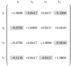
(c) $\bm{\eta}_{4\times 4}$

Figure 1: Computing Eells measure for Figure 2.

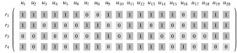
Figure 2: Preference matrix $M_{4\times 20}$.

Example 1.

Matrix $M_{4\times 20}$ in Figure 2 shows the preferences of $20$ users ($u_{1},...,u_{20}$) for $4$ requirements ($r_{1},...,r_{4}$). Each element $m_{i,j}$ specifies whether requirement $r_{j}$ has been preferred by user $u_{i}$ ($m_{i,j}=1$) or not ($m_{i,j}=0$). Matrix $P_{4\times 4}$ (Figure 1(a)) and Matrix $\bar{P}_{4\times 4}$ (Figure 1(b)) show the strengths of causal relations among user preferences for requirements in $M_{4\times 8}$. For a pair of requirements $r_{i}$ and $r_{j}$ with $i\neq j$, an off-diagonal element $p_{i,j}$ ($\bar{p}_{i,j}$) of matrix $P_{4\times 4}$ ($\bar{P}_{4\times 4}$) denotes the strength of a positive (negative) causal relation from $r_{i}$ to $r_{j}$. For diagonal elements of $P_{4\times 4}$ ($\bar{P}_{4\times 4}$) on the other hand, we have $p_{i,i}=p(r_{i}|r_{i})=1$ ($\bar{p}_{i,i}=p(r_{i}|\bar{r}_{i})=0$). Hence, subtracting each element $\bar{p}_{i,j}$ from its corresponding element $p_{i,j}$, where $i\neq j$, gives Eells causal strength $\eta_{i,j}$ for the value dependency from $r_{i}$ to $r_{j}$. Diagonal elements, however, may be ignored as they denote self-causation; $p(r_{i}|r_{i})=1$.

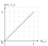
(a)

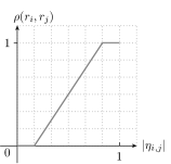
(b)

(c) Sample membership functions for value dependencies.

The strength of an explicit dependency from a requirement $r_{i}$ to $r_{j}$ is computed by (10), which gives a mapping from Eells measure $\eta_{i,j}$ to $\rho:R\times R\rightarrow[0,1]$ (Figure 2(c)). As given by (11), $\eta_{i,j}>0$ indicates that the strength of the positive causal relation from $r_{i}$ to $r_{j}$ is greater than the strength of its corresponding negative relation: $p(r_{i}|r_{j})>p(r_{i}|\neg r_{j})$; the quality of $(r_{i},r_{j})$ is positive ($\sigma(r_{i},r_{j})=+$). Similarly, $\eta_{i,j}<0$ indicates $p(r_{i}|\neg r_{j})>p(r_{i}|r_{j})\rightarrow\sigma(r_{i},r_{j})=-$. Also, $p(r_{i}|r_{j})-p(r_{i}|\neg r_{j})=0$ specifies that the quality of the zero-strength dependency $(r_{i},r_{j})$ is non-specified ($\sigma(r_{i},r_{j})=\pm$).

$$\rho(r_{i},r_{j})=|\eta_{i,j}|$$ (10)

$$\sigma(r_{i},r_{j})=\begin{cases}+&\text{if }\phantom{s}\eta_{i,j}>0\\ -&\text{if }\phantom{s}\eta_{i,j}<0\\ \pm&\text{if }\phantom{s}\eta_{i,j}=0\\ \end{cases}$$ (11)

Different membership functions may be adopted to account for the preferences of decision makers, e.g. the membership function in Figure III-A may be used to ignore “very weak” value dependencies while “very strong” dependencies are considered as full strength relations, $\rho(r_{i},r_{j})=1$.

III-B Modeling Value Dependencies

Fuzzy logic has been widely adopted in decision making [33] to capture the imprecision of real-world problems [80, 81, 82, 83, 84, 85]. In Software Engineering, fuzzy graphs have demonstrated useful in modeling the imprecision of dependency relations in software [86, 35, 21]. Ngo-The et al. used fuzzy graphs for modeling dependency satisfaction in software release planning [35] and capturing the imprecision of coupling dependencies among software requirements [21]. Also, Wang et al. [22] exploited fuzzy logic to capture the strengths of dependency relations among requirements. In this section, we discuss modeling value dependencies among requirements by fuzzy graphs. We further use the algebraic structure of fuzzy graphs to compute the overall influences of requirements on the values of each other.

III-B1 Value Dependency Graphs

To account for the imprecision of value dependencies, we have introduced Value Dependency Graphs (VDGs) based on fuzzy graphs for modeling value dependencies and their characteristics. We have specially modified the classical definition of fuzzy graphs to consider not only the strength but also the quality (positive or negative) of value dependencies as given by Definition 1.

Definition 1.

The Value Dependency Graph (VDG) is a signed directed fuzzy graph [87] $G=(R,\sigma,\rho)$ where, requirements $R:\{r_{1},...,r_{n}\}$ constitutes the graph nodes. Also, the qualitative function $\sigma(r_{i},r_{j})\rightarrow\{+,-,\pm\}$ and the membership function $\rho:(r_{i},r_{j})\rightarrow[0,1]$ denote the quality and the strength of the explicit value dependency (edge of the graph) from $r_{i}$ to $r_{j}$ receptively. Moreover, $\rho(r_{i},r_{j})=0$ denotes the absence of any explicit value dependency from $r_{i}$ to $r_{j}$. In that case we have $\sigma(r_{i},r_{j})=\pm$, where $\pm$ denotes the quality of the dependency is non-specified; in Figure 3, $\sigma(r_{1},r_{2})=+$ and $\rho(r_{1},r_{2})=0.4$ specifies a positive value dependency from $r_{1}$ to $r_{2}$ with strength $0.4$.

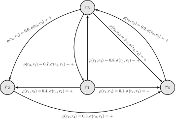
Figure 3: A sample value dependency graph.

III-B2 Value Dependencies in VDGs

In Section III-A we introduced an automated technique for the identification of explicit value dependencies and their characteristics (quality and strength) from user preferences. Definition 2 provides a more comprehensive definition of value dependencies that includes both explicit and implicit value dependencies among the requirements of software based on the algebraic structure of fuzzy graphs.

Definition 2.

Value Dependencies. A value dependency in a value dependency graph $G=(R,\sigma,\rho)$ is defined as a sequence of requirements $d_{i}:\big{(}r(0),...,r(k)\big{)}$ such that $\forall r(j)\in d_{i}$, $1\leq j\leq k$ we have $\rho\big{(}r(j-1),r(j)\big{)}\neq 0$. $j\geq 0$ is the sequence of the $j^{th}$ requirement (node) denoted as $r(j)$ on the dependency path. A consecutive pair $\big{(}r(j-1),r(j)\big{)}$ specifies an explicit value dependency.

$$\forall d_{i}:\big{(}r(0),...,r(k)\big{)}:\rho(d_{i})=\bigwedge_{j=1}^{k}\text{ }\rho\big{(}r(j-1),r(j)\big{)}$$ (12)

$$\forall d_{i}:\big{(}r(0),...,r(k)\big{)}:\sigma(d_{i})=\prod_{j=1}^{k}\text{ }\sigma\big{(}r(j-1),r(j)\big{)}$$ (13)

Equation (12) computes the strength of a value dependency $d_{i}:\big{(}r(0),...,r(k)\big{)}$ by finding the strength of the weakest of $k$ explicit dependencies on $d_{i}$. $\wedge$ denotes fuzzy AND operation [88]. The quality (positive or negative) of a value dependency $d_{i}:\big{(}r(0),...,r(k)\big{)}$ is calculated by qualitative serial inference [89, 90, 91] as given by (13) and Table II. Inferences in Table II are informally proved by Wellman [90] and Kleer [89].

TABLE II: Qualitative serial inference in VDGs.

$\sigma\big{(}r(j-1),r(j),r(j+1)\big{)}$		$\sigma\big{(}r(j),r(j+1)\big{)}$
		$+$	$-$	$\pm$ [b]
$\sigma\big{(}r(j-1),r(j)\big{)}$	$+$	$+$	$-$	$\pm$ [t]
	$-$	$-$	$+$	$\pm$
	$\pm$	$\pm$	$\pm$	$\pm$

Let $D=\{d_{1},d_{2},...,d_{m}\}$ be the set of all value dependencies from $r_{i}\in R$ to $r_{j}\in R$ in a VDG $G=(R,\sigma,\rho)$, where positive and negative dependencies can simultaneously exist from $r_{i}$ to $r_{j}$. The strength of all positive dependencies from $r_{i}$ to $r_{j}$, denoted by $\rho^{+\infty}(r_{i},r_{j})$, is calculated by (14), that is to find the strongest positive dependency [33] from $r_{i}$ to $r_{j}$. Fuzzy operators $\wedge$ and $\vee$ denote Zadeh’s [88] AND and OR operations respectively. Analogously, the strength of all negative value dependencies from $r_{i}$ to $r_{j}$ is denoted by $\rho^{-\infty}(r_{i},r_{j})$ and calculated by (15).

$$\rho^{+\infty}(r_{i},r_{j})=\bigvee_{d_{m}\in D,\sigma(d_{m})=+}\text{ }\rho(d_{m})$$ (14)

$$\rho^{-\infty}(r_{i},r_{j})=\bigvee_{d_{m}\in D,\sigma(d_{i})=-}\text{ }\rho(d_{m})$$ (15)

$$I_{i,j}=\rho^{+\infty}(r_{i},r_{j})-\rho^{-\infty}(r_{i},r_{j})$$ (16)

A brute-force approach to computing $\rho^{+\infty}(r_{i},r_{j})$ or $\rho^{-\infty}(r_{i},r_{j})$ needs to calculate the strengths of all paths from $r_{i}$ to $r_{j}$, which is of $O(n!)$ for $n$ requirements. To reduce this complexity, we have devised a modified version of Floyd-Warshall [92] algorithm (Algorithm 1), that computes $\rho^{+\infty}(r_{i},r_{j})$ and $\rho^{-\infty}(r_{i},r_{j})$ for all pairs of requirements $(r_{i},r_{j}),\text{ }r_{i},r_{j}\in R:\{r_{1},...,r_{n}\}$ in $O(n^{3})$. For each pair of requirements $(r_{i},r_{j})$ in a VDG $G=(R,\sigma,\rho)$, lines $18$ to $35$ of Algorithm 1 find the strength of all positive (negative) value dependencies from $r_{i}$ to $r_{j}$. The overall strength of all positive and negative value dependencies from $r_{i}$ to $r_{j}$ is referred to as the Influence of $r_{j}$ on the value of $r_{i}$ and denoted by $I_{i,j}$. $I_{i,j}$, as in (16), is computed by deducting the strength of all negative value dependencies from $r_{i}$ to $r_{j}$ ($\rho^{-\infty}(r_{i},r_{j})$) from the strength of all positive value dependencies from $r_{i}$ to $r_{j}$ ($\rho^{+\infty}(r_{i},r_{j})$). Therefore, $I_{i,j}>0$ ($I_{i,j}<0$) states that $r_{j}$ positively (negatively) influences the value of $r_{i}$.

0:  VDG $G=(R,\sigma,\rho)$ 0:  $\rho^{+\infty},\rho^{-\infty}$ 1:  for each $r_{i}\in R$ do 2:     for each $r_{j}\in R$ do 3:        $\rho^{+\infty}(r_{i},r_{j})\leftarrow\rho^{-\infty}(r_{i},r_{j})\leftarrow-\infty$ 4:     end for 5:  end for 6:  for each $r_{i}\in R$ do 7:     $\rho(r_{i},r_{i})^{+\infty}\leftarrow\rho(r_{i},r_{i})^{-\infty}\leftarrow 0$ 8:  end for 9:  for each $r_{i}\in R$ do 10:     for each $r_{j}\in R$ do 11:        if $\sigma(r_{i},r_{j})=+$ then 12:           $\rho^{+\infty}(r_{i},r_{j})\leftarrow\rho(r_{i},r_{j})$ 13:        else if $\sigma(r_{i},r_{j})=-$ then 14:           $\rho^{-\infty}(r_{i},r_{j})\leftarrow\rho(r_{i},r_{j})$ 15:        end if 16:     end for 17:  end for 18:  for each $r_{k}\in R$ do 19:     for each $r_{i}\in R$ do 20:        for each $r_{j}\in R$ do 21:           if $min\big{(}\rho^{+\infty}(r_{i},r_{k}),\rho^{+\infty}(r_{k},r_{j})\big{)}>\rho^{+\infty}(r_{i},r_{j})$ then 22:              $\rho^{+\infty}(r_{i},r_{j})\leftarrow min(\rho^{+\infty}(r_{i},r_{k}),\rho^{+\infty}(r_{k},r_{j}))$ 23:           end if 24:           if $min\big{(}\rho^{-\infty}(r_{i},r_{k}),\rho^{-\infty}(r_{k},r_{j})\big{)}>\rho^{+\infty}(r_{i},r_{j})$ then 25:              $\rho^{+\infty}(r_{i},r_{j})\leftarrow min(\rho^{-\infty}(r_{i},r_{k}),\rho^{-\infty}(r_{k},r_{j}))$ 26:           end if 27:           if $min\big{(}\rho^{+\infty}(r_{i},r_{k}),\rho^{-\infty}(r_{k},r_{j})\big{)}>\rho^{-\infty}(r_{i},r_{j})$ then 28:              $\rho^{-\infty}(r_{i},r_{j})\leftarrow min(\rho^{+\infty}(r_{i},r_{k}),\rho^{-\infty}(r_{k},r_{j}))$ 29:           end if 30:           if $min\big{(}\rho^{-\infty}(r_{i},r_{k}),\rho^{+\infty}(r_{k},r_{j})\big{)}>\rho^{-\infty}(r_{i},r_{j})$ then 31:              $\rho^{-\infty}(r_{i},r_{j})\leftarrow min(\rho^{-\infty}(r_{i},r_{k}),\rho^{+\infty}(r_{k},r_{j}))$ 32:           end if 33:        end for 34:     end for 35:  end for

Algorithm 1 Strengths of value dependencies.

Example 2.

Let $D=\{d_{1}:(r_{1},r_{2},r_{4}),d_{2}:(r_{1},r_{3},r_{4}),d_{3}:(r_{1},r_{4})\}$ be the value dependencies from $r_{1}$ to $r_{4}$ in Figure 3. Using (13), qualities of $d_{1}$ to $d_{3}$ are: $\sigma(d_{1})=\Pi(+,+)=+$, $\sigma(d_{2})=\Pi(+,+)=+$, and $\sigma(d_{3})=\Pi(-)=-$. Strengths are calculated by (12) as: $\rho(d_{1})=\wedge\big{(}\rho(r_{1},r_{2}),\rho(r_{2},r_{4})\big{)}=min(0.4,0.3)$, $\rho(d_{2})=\wedge\big{(}\rho(r_{1},r_{3}),\rho(r_{3},r_{4})\big{)}=min(0.8,0.8)$, $\rho(d_{3})=min(0.1)$. Then, using (14) and (15, we have $\rho(r_{1},r_{4})^{+\infty}=\vee(\rho(d_{1}),\rho(d_{2}))=max(0.3,0.8)$ and $\rho^{-\infty}(r_{1},r_{4})=max(\rho(d_{3}))$. Therefore, $I_{1,4}=\rho(r_{1},r_{4})^{+\infty}-\rho(r_{1},r_{4})^{-\infty}=0.7$. Table III lists influences of requirements in the VDG of Figure 3 on the value of each other.

TABLE III: Overall influences computed for VDG of Figure 3.

$I_{i,j}$	$r_{1}$	$r_{2}$	$r_{3}$	$r_{4}$
$r_{1}$	$0.0$	$0.5$	$0.7$	$0.7$
$r_{2}$	$0.2$	$0.0$	$0.2$	$0.3$
$r_{3}$	$0.6$	$0.5$	$0.0$	$0.7$
$r_{4}$	$0.2$	$0.2$	$0.2$	$0.0$

Definition 3.

Value Dependency Level (VDL) and Negative Value Dependency Level (NVDL). Let $G=(R,\sigma,\rho)$ be a VDG with $R=\{r_{1},...,r_{n}\}$, $k$ be the total number of explicit value dependencies in $G$, and $m$ be the total number of negative explicit value dependencies. Then the VDL and NVDL of $G$ are derived by (17) and (18) respectively.

$$VDL(G)=\frac{k}{{}^{n}\!P_{2}}=\frac{k}{n(n-1)}$$ (17)

$$NVDL(G)=\frac{m}{k}$$ (18)

Example 3.

For the value dependency graph $G$ of Figure 3, we have $n=4$, $k=8$, and $m=1$. $VDL(G)$ is derived by (17) as: $VDL(G)=\frac{8}{4\times 3}=\frac{8}{12}\approxeq 0.67$. Also we have from Equation (18), $NVDL(G)=\frac{1}{8}=0.125$.

IV Integrating Value Dependencies

IV-A Overall Value of a Requirement Subset

This section details our proposed measure of value, i.e. overall value (OV), for the economic worth of a requirement subset. OV takes into account user preferences for the selected requirements as well as the impacts of value dependencies on the values of requirements. Value dependencies, as explained in Section III-A, are identified based on causal relations among user preferences. Section III-A presented an automated technique for the identification of value dependencies among requirements; Algorithm 1 was used to infer implicit value dependencies and compute the influences of requirements on the values of each other based on the algebraic structure of fuzzy graphs. To compute the overall values of the selected requirements, (IV-A)-(20) give the penalty of ignoring (selecting) requirements with positive (negative) influence on the values of the selected requirements. $\theta_{i}$ in this equation denotes the penalty for a requirement $r_{i}$, $n$ denotes the number of requirements, and $x_{j}$ specifies whether requirement $r_{j}$ is selected ($x_{j}=1$) or not ($x_{j}=0$). Also, $I_{i,j}$, as in (16), gives the positive or negative influence of $r_{j}$ on the value of $r_{i}$.

$$\theta_{i}= \displaystyle\bigvee_{j=1}^{n}\bigg{(}\frac{x_{j}\big{(}\lvert I_{i,j}\rvert-I_{i,j}\big{)}+(1-x_{j})\big{(}\lvert I_{i,j}\rvert+I_{i,j}\big{)}}{2}\bigg{)}=$$

$$\displaystyle\bigvee_{j=1}^{n}\bigg{(}\frac{\lvert I_{i,j}\rvert+(1-2x_{j})I_{i,j}}{2}\bigg{)},i\neq j=1,...,n$$ (19)

$$x_{j}\in\{0,1\},j=1,...,n$$ (20)

We made use of the algebraic structure of fuzzy graphs for computing the influences of requirements on the values of each other as explained in Section III-B. Accordingly, $\theta_{i}$ is computed using the fuzzy OR operator which is to take supremum over the strengths of all ignored positive dependencies and selected negative dependencies of $r_{i}$ in its corresponding value dependency graph. Overall values of the selected requirements thus can be computed by (22), where $v_{i}^{\prime}$ denotes the overall value of a requirement $r_{i}$, $E(v_{i})$ specifies the expected value of $r_{i}$, and $\theta_{i}$ denotes the penalty of ignoring (selecting) positive (negative) value dependencies of $r_{i}$. Equation (23) derives the overall value of $n$ requirements, where cost and expected value of a requirements $r_{i}$ are denoted by $c_{i}$ and $E(v_{i})$ respectively. Decision variable $x_{i}$ specifies whether $r_{i}$ is selected ($x_{i}=1$) or not ($x_{i}=0$). $E(V_{i})$ is computed by (43), where $v_{i}$ denotes the estimated value of $r_{i}$. Also $p(r_{i})$ ($p(\bar{r_{i}})$) specify the probability that users select (ignore) $r_{i}$.

$$E(v_{i})=p(r_{i})\times v_{i}+p(\bar{r_{i}})\times 0=p(r_{i})\times v_{i}$$ (21)

For a requirement $r_{i}$, $\theta_{i}$ specifies the penalty of ignoring (selecting) requirements with positive (negative) influence on the expected value of $r_{i}$. $\theta_{i}v_{i}$ in (23) therefore, gives the value loss for a requirement $r_{i}$ as a result of ignoring (selecting) requirements that positively (negatively) impact user preferences for $r_{i}$ and consequently its expected value.

$$v_{i}^{\prime}=(1-\theta_{i})E(v_{i})$$ (22)

$$OV=\sum_{i=1}^{n}x_{i}(1-\theta_{i})E(v_{i}),\textit{ }x_{i}\in\{0,1\}$$ (23)

Example 4.

Consider finding penalties for requirements of Figure 3, where $r_{4}$ is not selected ($x_{1}=x_{2}=x_{3}=1,x_{4}=0$). From Table III we have $I_{1,4}=I_{3,4}=0.7,I_{2,4}=0.3,I_{4,4}=0.0$. As such, based on (IV-A) penalties are computed: $\theta_{1}=\vee(\frac{\lvert 0.0\rvert+(1-2(1))(0.0)}{2}$, $\frac{\lvert 0.45\rvert+(1-2(1))(0.5)}{2}$, $\frac{\lvert 0.7\rvert+(1-2(1))(0.7)}{2}$, $\frac{\lvert 0.7\rvert+(1-2(0))(0.7)}{2})=0.7$. Similarly, we have $\theta_{2}=0.3,\theta_{3}=0.7$. Therefore, the overall value of the selected requirements $r_{1},r_{2},r_{3}$ is derived by (23) as: $OV(s_{1})=(1-0.7)E(v_{1})+(1-0.3)E(v_{2})+(1-0.7)E(v_{3})$.

IV-B The Integer Programming Model

This section presents our proposed integer programming model for optimizing the overall value of software. The overall value of a software requirement subset, as given by (23), considers user preferences and the impacts of value dependencies on the expected values of the selected requirements. Equations (24)-(29) give our proposed integer programming model as a main component of DARS. In these equations, $x_{i}$ is a selection variable denoting whether a requirement $r_{i}$ is selected ($x_{i}=1$) or ignored ($x_{i}=0$). Also $\theta_{i}$ in (IV-A) specifies the penalty of a requirement $r_{i}$, which is the extent to which the expected value of $r_{i}$ is impacted by ignoring (selecting) requirements with positive (negative) influences on the value of $r_{i}$. Constraint (26) accounts for precedence dependencies among requirements and the value implications of those dependencies. Moreover, for a requirement $r_{i}$, $\theta_{i}$ depends on the selection variable $x_{j}$ and the strength of positive (negative) value dependencies as given by (IV-A). As $I_{i,j}$ is computed by (16), we can restate $\theta_{i}$ as a function of $x_{j}$: $\theta_{i}=f(x_{j})$. The objective function (24), thus, can be restated as $\text{Maximize }\sum_{i=1}^{n}x_{i}E(v_{i})-x_{i}f(x_{j})E(v_{i})$ where $x_{i}f(x_{j})E(v_{i})$ is a quadratic non-linear expression [93].

$$\text{Maximize }\sum_{i=1}^{n}x_{i}(1-\theta_{i})E(v_{i})$$ (24)

$$\text{Subject to}\sum_{i=1}^{n}c_{i}x_{i}\leq b$$ (25)

$$\begin{cases}x_{i}\leq x_{j}&r_{j}\text{ precedes }r_{i}\\[2.0pt] x_{i}\leq 1-x_{j}&r_{i}\text{ conflicts with }r_{j},\text{ }i\neq j=1,...,n\\[2.0pt] \end{cases}$$ (26)

$$\theta_{i}\geq\bigg{(}\frac{\lvert I_{i,j}\rvert+(1-2x_{j})I_{i,j}}{2}\bigg{)},i\neq j=1,...,n$$ (27)

$$\text{ }x_{i}\in\{0,1\},i=1,...,n$$ (28)

$$\text{ }0\leq\theta_{i}\leq 1,i=1,...,n$$ (29)

Equations (24)-(27), on the other hand, denote a convex optimization problem as the model maximizes a concave objective function with linear constraints. Convex optimization problems are solvable [93, 94]. However, for problems of moderate to large sizes, Integer Linear Programming (ILP) models are preferred [95] as they can be efficiently solved, despite the inherent complexity of NP-hard problems, due to the advances in solving ILP models and availability of efficient tools such as ILOG CPLEX for that purpose.

$$\text{Maximize }\sum_{i=1}^{n}x_{i}E(v_{i})-y_{i}E(v_{i})$$ (30)

$$\text{Subject to}\sum_{i=1}^{n}c_{i}x_{i}\leq b$$ (31)

$$\begin{cases}x_{i}\leq x_{j}&r_{j}\text{ precedes }r_{i}\\[2.0pt] x_{i}\leq 1-x_{j}&r_{i}\text{ conflicts with }r_{j},\text{ }i\neq j=1,...,n\end{cases}$$ (32)

$$\theta_{i}\geq\bigg{(}\frac{\lvert I_{i,j}\rvert+(1-2x_{j})I_{i,j}}{2}\bigg{)},i\neq j=1,...,n$$ (33)

$$-g_{i}\leq x_{i}\leq g_{i},i=1,...,n$$ (34)

$$1-(1-g_{i})\leq x_{i}\leq 1+(1-g_{i}),i=1,...,n$$ (35)

$$-g_{i}\leq y_{i}\leq g_{i},i=1,...,n$$ (36)

$$-(1-g_{i})\leq(y_{i}-\theta_{i})\leq(1-g_{i}),i=1,...,n$$ (37)

$$\text{ }0\leq y_{i}\leq 1,i=1,...,n$$ (38)

$$\text{ }0\leq\theta_{i}\leq 1,i=1,...,n$$ (39)

$$\text{ }x_{i},g_{i}\in\{0,1\},i=1,...,n$$ (40)

This motivates us to consider deriving an ILP version of the model as given by (30). In doing so, non-linear expression $x_{i}\theta_{i}$ is substituted by linear expression $y_{i}$ ($y_{i}=x_{i}\theta_{i}$). As such, either $a:(x_{i}=0,y_{i}=0)$, or $b:(x_{i}=1,y_{i}=\theta_{i})$ occur. To capture the relation between $\theta_{i}$ and $y_{i}$ in a linear form, we have made use of an auxiliary variable $g_{i}=\{0,1\}$ and (34)-(38) are added to the original model. As such, we have either $(g_{i}=0)\rightarrow a$, or $(g_{i}=1)\rightarrow b$. Therefore, (30)-(40), referred to as DARS-ILP, is linear and can be efficiently solved [93], even for large scale requirement sets, by existing commercial solvers such as IBM CPLEX.

IV-C The Complementary Model

There might be situations where identifying value dependencies is hard, e.g, when collecting user preferences is costly. In such cases, value dependencies cannot be considered in requirement selection, that may lead to ignoring (selecting) the requirements with significant positive (negative) influences on the values of the selected requirements and therefore result in value loss. When the impacts of negative value dependencies are negligible, value loss induced by ignoring positive value dependencies can be mitigated by trying to select as many requirements as possible, respecting the budget. On this basis, we have proposed a complementary (ILP) model of DARS that reduces the chances that the requirements with positive influences on the values of the selected requirements are ignored.

$$f_{1}(n,x_{i},E(v_{i}))=\sum_{i=1}^{n}x_{i}E(v_{i})$$ (41)

$$f_{2}(n,x_{i})=\sum_{i=1}^{n}x_{i}$$ (42)

$$E(v_{i})=p(r_{i})v_{i}$$ (43)

Equations (44)-(47) give a multi-objective (bi-objective) formulation of the blind model of DARS, which aims to simultaneously maximize the utility functions $f_{1}$ and $f_{2}$ while respecting the budget constraint (45) and the precedence constraints (46). The utility function $f_{1}$ in (41) concerns with the expected value of the selected requirements while the utility function $f_{2}$ specifies the number of the selected requirements as given by (42). In these equations, $b$ denotes the budget and $x_{i}$ is a decision variable specifying if requirement $r_{i}$ is selected ($x_{i}=1$) or not ($x_{i}=0$). Also, $c_{i}$ and $E(v_{i})$ denote the estimated cost and the expected value of $r_{i}$ respectively. $E(v_{i})$ is computed by (43) where $v_{i}$ is the estimated value of $r_{i}$ and $p(r_{i})$ denotes the probability that users select $r_{i}$. The optimization model (44)-(47), aims to find a requirement subset with the highest values for utility functions $f_{1}$ and $f_{2}$ while keeping the cost within the budget and respecting the precedence constraints (46). However, maximizing the number of the selected requirements (the utility function $f_{2}$) may conflict with maximizing the expected value of the selected requirements (the utility function $f_{1}$).

Hence, finding an optimal subset without knowing the preference of a decision make is not possible; all Pareto Optimal [44] subsets found by the optimization model (44)-(47) are considered to be equally good. In a Pareto optimal (Non-Dominated) subset found by the model, none of the utility functions $f_{1}$ or $f_{2}$ can be improved in value without degrading the other. The optimization model (44)-(47) can be solved in different ways, as discussed in [96], depending on the viewpoints of the decision makers and, thus, there exist different solution philosophies when solving them.

$$\text{Maximize }\{f_{1}(n,x_{i},E(v_{i})),f_{2}(n,x_{i})\}$$ (44)

$$\text{Subject to}\sum_{i=1}^{n}x_{i}c_{i}\leq b$$ (45)

$$\begin{cases}x_{i}\leq\text{$x_{j}$}&r_{j}\text{ precedes }r_{i}\\[5.0pt] x_{i}\leq 1-\text{$x_{j}$}&r_{i}\text{ conflicts with }r_{j},\text{ }i\neq j=1,...,n\\[5.0pt] \end{cases}$$ (46)

$$\text{ }x_{i}\in\{0,1\},i=1,...,n$$ (47)

We reformulate the complementary model of DARS as a single-objective model in (48)-(52), that aims to avoid ignoring requirements (maximizing $f_{2}$) as long as the budget constraint (49) is respected and the utility function $f_{1}$ is partly satisfied by guaranteeing a lower-bound $V$ for the expected value of the optimal subset. $V$ will be specified by decision makers. The conflict between the utility functions $f_{1}$ and $f_{2}$, thus, is reconciled by maximizing $f_{2}$ while ensuring a lower-bound for $f_{1}$. Moreover, precedence dependencies among the requirements are captured by (51), where $x_{i}\leq x_{j}$ states that a requirement $r_{i}$ requires $r_{j}$ while $x_{i}\leq(1-x_{j})$ means that $r_{i}$ conflicts with $r_{j}$.

$$\text{Maximize }f_{1}(n,x_{i},E(v_{i}))$$ (48)

$$\text{Subject to}\sum_{i=1}^{n}x_{i}c_{i}\leq b$$ (49)

$$f_{2}(n,x_{i})\geq V$$ (50)

$$\begin{cases}x_{i}\leq x_{j}&r_{j}\text{ precedes }r_{i}\\[5.0pt] x_{i}\leq 1-x_{j}&r_{i}\text{ conflicts with }r_{j},\text{ }i\neq j=1,...,n\\[5.0pt] \end{cases}$$ (51)

$$\text{ }x_{i}\in\{0,1\},i=1,...,n$$ (52)

Finally, the complementary ILP model of DARS, as given by (48)-(52), is linear and therefore can be efficiently solved [93], even for large scale requirement sets, by the existing commercial solvers such as IBM CPLEX [97]. We have implemented, solved, the model using the Concert Technology and the JAVA API of IBM CPLEX [97].

V Simulations

This section demonstrates the effectiveness of the ILP model of DARS through simulations. The model accounts for user preferences using the expected values of the requirements ($E(v_{i})$) as discussed before. But the interplay between user preferences and value dependencies may interfere with studying the impact of value dependencies on the effectiveness of DARS. This may, particularly, occur when value dependencies are found among frequently preferred requirements with higher values. To merely study the impacts of value dependencies, we have substituted, without loss of generality, the expected values of requirements $(E(v_{i}))$ with their corresponding estimated values ($v_{i}$) in (30)-(40), thus factoring out the impact of user preferences from simulations.

We have further, considered different budgets and levels of precedence dependencies in simulations. Simulations were carried out for $27$ requirements of a real-world software with the estimated values and costs scaled into $[0,20]$ (Table IV). Value dependencies and precedence dependencies among the requirements were randomly generated. The Java API of IBM CPLEX was used to implement the optimization models of the BK, PCBK, and DARS. Also, the callable library ILOG CPLEX 12.6.2 was used to run these models on a machine with a Core i7-2600 3.4 GHz processor and 16 GB of RAM.

TABLE IV: The estimated costs and values of the requirements.

$r_{i}$	$c_{i}$	$v_{i}$	$r_{i}$	$c_{i}$	$v_{i}$
$r_{1}$	05.00	10.00	$r_{15}$	15.00	08.00
$r_{2}$	20.00	20.00	$r_{16}$	13.00	10.00
$r_{3}$	00.00	04.00	$r_{17}$	14.00	06.00
$r_{4}$	10.00	17.00	$r_{18}$	03.00	10.00
$r_{5}$	01.00	03.00	$r_{19}$	10.00	20.00
$r_{6}$	20.00	20.00	$r_{20}$	07.00	20.00
$r_{7}$	06.00	15.00	$r_{21}$	12.00	15.00
$r_{8}$	05.00	09.00	$r_{22}$	15.00	20.00
$r_{9}$	16.00	20.00	$r_{23}$	08.00	20.00
$r_{10}$	10.00	16.00	$r_{24}$	02.00	05.00
$r_{11}$	04.00	20.00	$r_{25}$	10.00	00.00
$r_{12}$	03.00	10.00	$r_{26}$	00.00	00.00
$r_{13}$	05.00	06.00	$r_{27}$	01.00	00.00
$r_{14}$	07.00	08.00
Sum	112.00	178.00	-	110.00	134.00

Requirement selection was performed for different percentages of budget ($\%\text{Budget}=\{1,...,100\}$), value dependency levels (VDL $\in[0,1]$), negative value dependency levels (NVDL $\in[0,1]$), precedence dependency levels (PDL $\in[0,1]$), and negative precedence dependency levels (NPDL $\in[0,1]$). PDL and NPDL were computed by (53) and (54) respectively to build random precedence graphs $G$ with $n=27$ nodes (requirements). In these equations, $k$ and $j$ denote the total number of precedence dependencies and the number of negative precedence dependencies respectively.

$$PDL(G)=\frac{k}{{}^{n}\!P_{2}}=\frac{k}{n(n-1)}$$ (53)

$$NPDL(G)=\frac{j}{k}$$ (54)

Table V lists our simulation settings designed to answers the following research questions.

• What is the impact of value dependencies on the performance of DARS in the presence of various budget constrains?

• What is the impact of negative value dependencies on the performance of DARS in the presence of various budget constrains?

• What is the impact of precedence dependencies on the performance of DARS in the presence of various budget constrains?

• What is the impact of negative precedence dependencies on the performance of DARS in the presence of various budget constrains?

• What is the impact of negative value dependencies on the performance of DARS in the presence of different levels of value dependencies?

• What is the impact of negative precedence dependencies on the performance of DARS for different levels of precedence dependencies?

To simulate value dependencies for a desired VDL and NVDL, uniformly distributed random numbers in $[-1,1]$ were generated, where the sign and magnitude of each number specified the quality and the strength of its corresponding explicit value dependency respectively. In a similar way, for a desired PDL and NPDL, random numbers in $\{-1,0,1\}$ were generated where $1$ ($-1$) specified a positive (negative) precedence dependency and $0$ denoted the absence of any precedence dependency from a requirement $r_{i}$ to $r_{j}$. Furthermore, percentages of the overall value of selected requirements ($\%$OV$=\frac{\text{OV}}{\sum_{i=1}^{27}v_{i}}$) were used to measure the performance of the simulated selection methods.

The performance of BK was, however, arbitrary as it does not consider precedence dependencies and therefore in many cases, depending on the PDL and NPDL, violates those dependencies giving infeasible solutions with no value ($\%\text{OV}=0$). On the other hand, the PCBK method enhances BK by considering precedence dependencies. As such, the PCBK method always outperforms the BK method giving higher or equal $\%$OV. Hence, we have mainly focused on comparing the performance of the PCBK and DARS methods. Moreover, Increase-Decrease methods were not simulated as they do not specify how to achieve the amount of increased or decreased values (Section II).

TABLE V: Performance simulations for the selection methods.

Simulation	$\%$Budget	VDL	NVDL	PDL	NPDL
I	[0,100]	[0,1]	0.00	0.02	0.00
II	[0,100]	0.15	[0,1]	0.02	0.00
III	[0,100]	0.15	0.00	[0,1]	0.00
IV	[0,100]	0.15	0.00	0.02	[0,1]
V	95	[0,1]	[0,1]	0.02	0.00
VI	95	0.15	0.00	[0,1]	[0,1]

V-A Value Dependencies vs Budget

To answer (RQ1), Simulation I in Table V was carried out for $\%$Budget $\in[0,100]$ and $VDL=[0,1]$. Figure 4 shows the percentages of accumulated value ($\%$AV) and overall value ($\%$OV) achieved from the selection methods. As expected, BK ignored/violated precedence dependencies and generated infeasible solutions with $\%$AV=$\%$OV$=0$ in most cases (Figure 4(a) and Figure 4(b)). It is clear that with no precedence dependencies (PDL=0), BK and PCBK will perform the same. We further, observed (Figure 4) that for a given $\%$Budget and NVLD=0 increasing VDL generally decreased $\%$OV achieved by all selection methods. The reason is increasing VDL increases the chances that the positive dependencies of a requirement are ignored, that may negatively influence the values of the selected requirements.

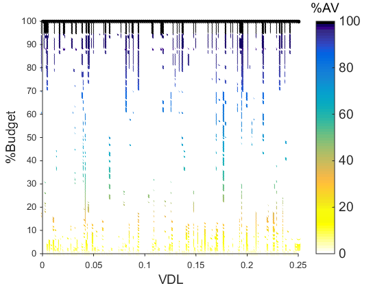
(a) $\%$AV(BK)

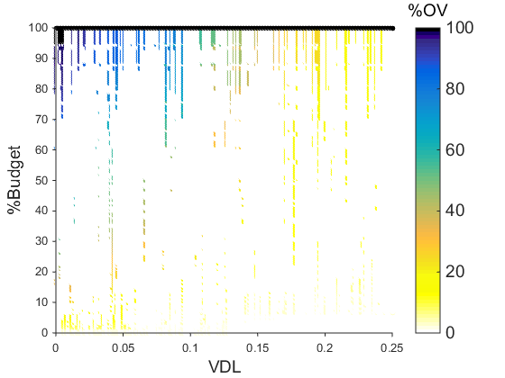
(b) $\%$OV(BK)

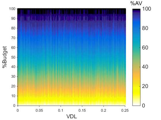
(c) $\%$AV(PCBK)

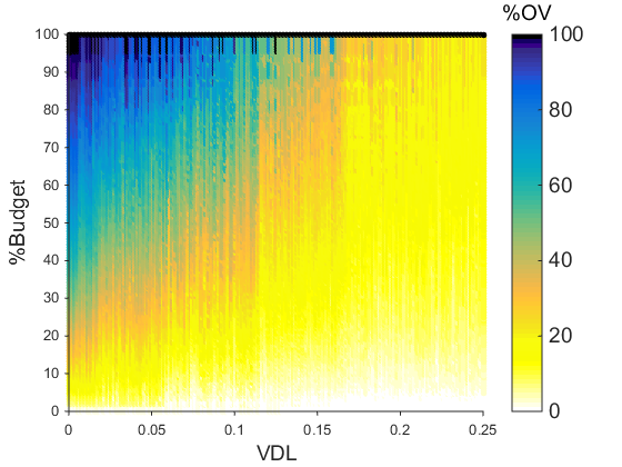
(d) $\%$OV(PCBK)

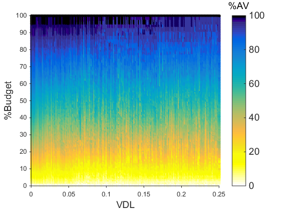
(e) $\%$AV(DARS)

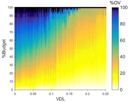
(f) $\%$OV(DARS)

Figure 4: Simulation I ($\%$Budget vs. VDL).

Figure 4 and Figure 5, also, show that DARS gives higher $\%$OV for all VDLs and $\%$Budget compared to the PCBK and BK methods. The reason is the ILP model of DARS considers value dependencies as well as the value implications of precedence dependencies while the BK method ignores dependencies all together, and the PCBK method only considers precedence dependencies. Figure 5 compares $\%$OV and $\%$AV provided by DARS against those of BK and PCBK for various $\%$Budget and VDLs. We have $\%\Delta$OV($m_{1}$,$m_{2}$)=$\%$OV($m_{1}$)$-\%$OV($m_{2}$) and $\%\Delta$AV($m_{1}$,$m_{2}$)=$\%$AV($m_{1}$)$-\%$AV ($m_{2}$) for selection methods $m_{1}$ and $m_{2}$. Our results demonstrated that DARS outperformed BK and PCBK by providing higher $\%$OV (Figure 5). Moreover, we observed that finding a requirement subset with the highest accumulated value conflicts with finding a subset with the highest overall value: to maximize OV and AV are conflicting objectives. This is demonstrated in many points in the graphs of Figure 5(d) and Figure 5(b), where for a given $\%$Budget and VDL, $\%\Delta$AV(DARS,PCBK) $<0$ while $\%\Delta$OV(DARS,PCBK) $>0$.

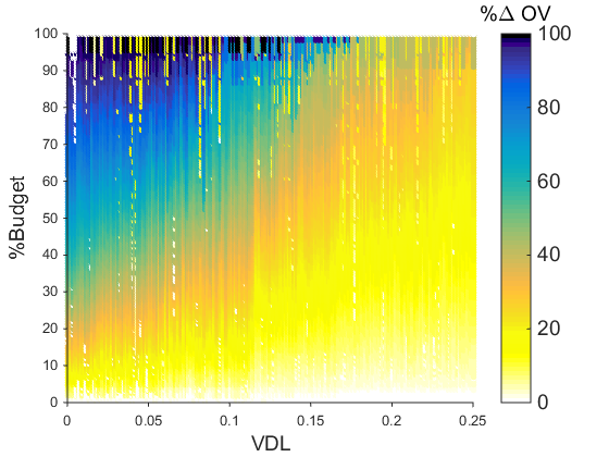
(a) $\%\Delta$OV(DARS,BK)

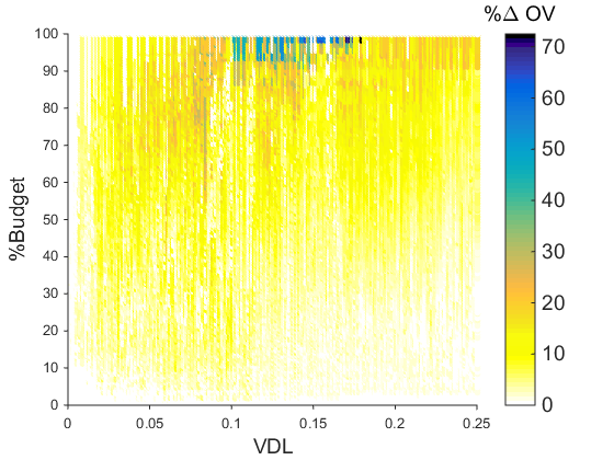
(b) $\%\Delta$OV(DARS,PCBK)

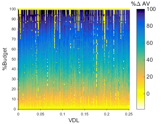
(c) $\%\Delta$AV(DARS,BK)

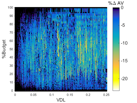
(d) $\%\Delta$AV(DARS,PCBK)

Figure 5: Simulation I ($\%$Budget vs. VDL).

V-B Negative Value Dependencies vs Budget

To answer (RQ2), Simulation II was performed for various budgets and NVDLs with settings in Table V. We observed that increasing NVDL resulted in arbitrary changes in $\%$OV achieved from PCBK and DARS. This is specified by (16) where increasing NVDL may arbitrarily increase or decrease the penalty of selecting or ignoring requirements depending on the strengths of positive and negative dependencies and the structure of the value dependency graph of the requirements.

Moreover, for $\%$Budget=100 and $NVDL\rightarrow 0$, we observed (Figure 6) that the maximum $\%$OV can be achieved in both PCBK and DARS methods. The reason is in such cases positive value dependencies do not matter as no requirement is excluded from the optimal subset due to the presence of sufficient budget.

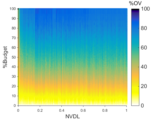
(a) $\%$OV(PCBK)

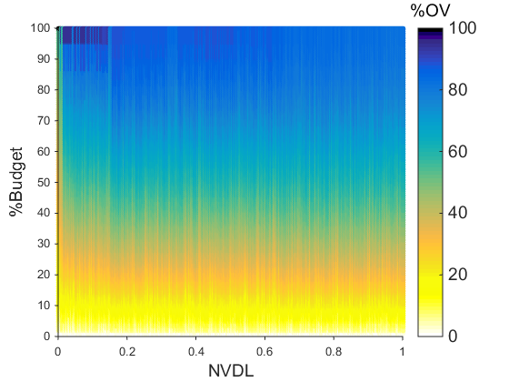
(b) $\%$OV(DARS)

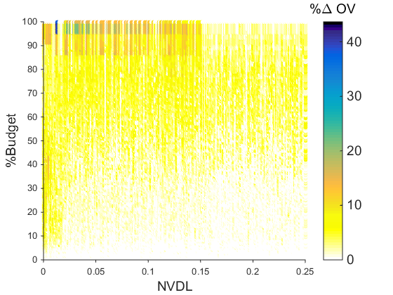
(c) $\%\Delta$OV(DARS,PCBK)

Figure 6: Simulation II ($\%$Budget vs. NVDL).

Nonetheless, with NVDL increase in Figure 6 the maximum $\%$OV cannot be achieved even with sufficient budget. The reason is in such cases even selecting requirements may reduce the values of other requirements due to negative value dependencies among them. We further, observed (Figure 6(c)) that, consistent with Simulation I, DARS always provided higher $\%$OV compared to PCBK. Also, the BK method failed to find feasible solutions in most simulations due to violating precedence dependencies.

V-C Precedence Dependencies vs Budget

To answer (RQ3), Simulation III was performed for various $\%$Budget and PDLs with settings in Table V. For a given VDL, we observed that increasing PDL generally resulted in decreasing the $\%$OV achieved from DARS (Figure 7(b)). The reason is increasing PDL reduces the number of feasible solutions that maintain the precedence constraints. This is also described as the selection deficiency problem (SDP) [12] where the efficiency of selection models is constrained by precedence dependencies. A similar effect was observed for PCBK (Figure 7(a)).

However, decreasing $\%$OV with PDL increase did not monotonically occur when PCBK was used; increasing PDL resulted in higher $\%$OV in some cases. Such arbitrary effects are more tangible in simulations with $\%\text{Budget}\geq 70$ and $vdl\leq 0.1$. The reason is PCBK ignores value dependencies. As such, even with fewer precedence constraints, PCBK may choose a solution with lower $\%$OV. On the contrary, DARS gave higher $\%$OV for smaller PDLs (Figure 7(b)). Figure 7(c) shows DARS outperformed PCBK. But, for PDL $\geq 0.15$, the number of feasible solutions was significantly reduced in both methods and the their performances converged, DARS lost its advantage.

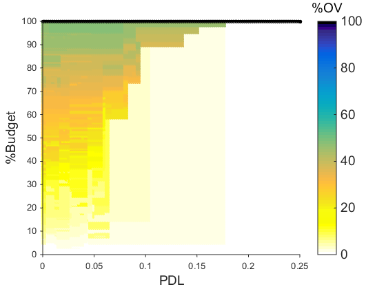
(a) $\%$OV(PCBK)

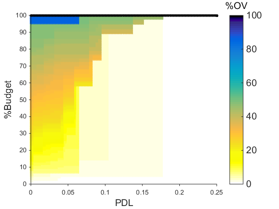
(b) $\%$OV(DARS)

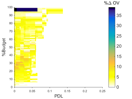
(c) $\%\Delta$OV(DARS,PCBK)

Figure 7: Simulation III ($\%$Budget vs. PDL).

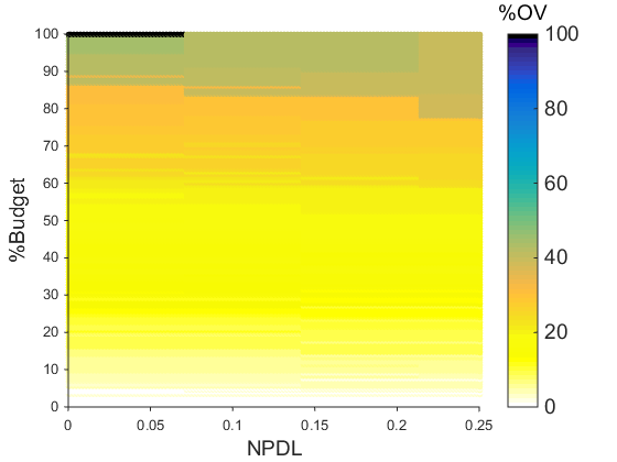
(a) $\%$OV(PCBK)

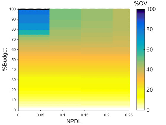
(b) $\%$OV(DARS)

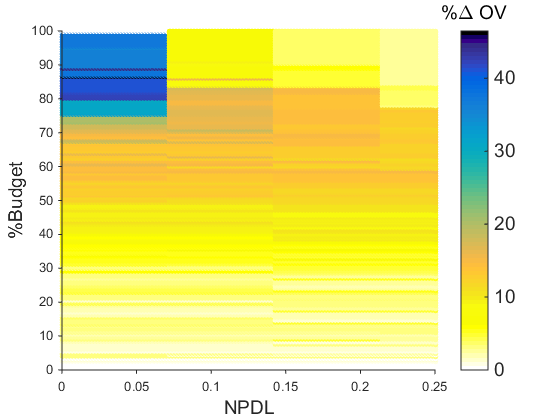
(c) $\%\Delta$OV(DARS,PCBK)

Figure 8: Simulation IV ($\%$Budget vs. NPDL).

V-D Negative Precedence Dependencies vs Budget

To answer (RQ4), Simulation IV was performed for different $\%$Budget and NPDLs. For both PCBK and DARS, increasing NPDL limited the number of feasible solutions while increasing the chances that certain requirements were selected. The former resulted in decreasing $\%$OV while the latter arbitrarily increased $\%$OV (8); consider requirements $r_{1}$, $r_{2}$, $r_{3}$, where there are negative precede dependencies from $r_{1}$ to $r_{2}$ ($x_{1}\leq(1-x_{2})$) and from $r_{2}$ to $r_{3}$, ($x_{2}\leq(1-x_{3})$): selecting $r_{3}$ results in ignoring $r_{2}$, which increases the chances that $r_{1}$ is selected.

We further, observed (Figure 8(c)) that DARS outperformed PCBK for up to around 46$\%$. Moreover, for $75\leq\%\text{Budget}<100$ and $NPDL\leq 0.15$, we observed that $\Delta(\text{PCBK},\text{BK})$ and $\Delta(\text{DARS},\text{PCBK})$ were the highest. The reason is DARS finds better solutions in the presence of fewer negative precedence constraints and more budget.

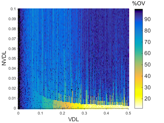
(a) $\%$OV(PCBK)

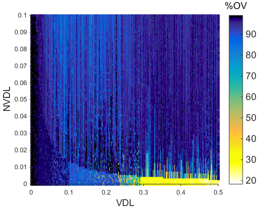
(b) $\%$OV(DARS)

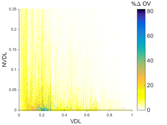
(c) $\%\Delta$OV(DARS,PCBK)

Figure 9: Simulation V (NVDL vs. VDL).

V-E Positive vs Negative Value Dependencies

To answer (RQ5), Simulation V was performed for different VDLs and NVDL with $\%\text{Budget}=95$, PDL=$0.02$, and NPDL =$0.0$ as given in Table V. The impact of VDL is shown to vary for smaller and larger NVDLs. For smaller NVDLs ($NVDL\leq 0.01$) increasing VDL monotonically decreased the $\%$OV provided by the selection methods. In other cases, however, increasing VDL was demonstrated to increase $\%$OV, although such increase was not monotonic. The reason is, as explained earlier, higher NVDLs increase the chances that simultaneous negative and positive value dependencies from a requirement $r_{i}$ to $r_{j}$ exist and therefore, negative value dependencies from $r_{i}$ to $r_{j}$ ($\rho(r_{i},r_{j})^{-\infty}$) mitigate the impact of positive dependencies from $r_{i}$ to $r_{j}$ ($\rho(r_{i},r_{j})^{+\infty}$) and vice versa. This reduces the overall influence of $r_{j}$ on $r_{i}$ based on (16). Hence, neither selecting nor ignoring $r_{j}$ does result in a significant loss in the value of $r_{i}$ and the $\%$OV of the selected subset of the requirements.

V-F Positive vs Negative Precedence Dependencies

To answer (RQ6), simulations for different PDLs and NPDLs were performed with settings of Simulation VI in Table V. Our simulations showed (Figure 10) that increasing PDL, in general, decreased the $\%$OV provided by the PCBK and DARS methods. This decrease, nevertheless, was not monotonic in the presence of negative precedence dependencies (NPDL$\neq 0$). The reason for this arbitrary impact of negative precedence dependencies was explained in detail in Section V-D. Our simulations showed that for any PDL, there exists a threshold $t$, where PCBK and DARS do not give any value for NPDLs $<t$. These thresholds increased as the PDL increased. This is more visible for PDL $\geq 0.1$. To further explain this, consider a requirement set $R=\{r_{1},r_{2}\}$ with equal costs and equal values, where $r_{1}$ requires $r_{2}$ (positive precedence dependency from $r_{1}$ to $r_{2}$) and $r_{2}$ requires $r_{1}$. This means we have $PDL=1$ and $NPDL=0$. As such, for $\%\text{Budget}<100$, either or both of the $r_{1}$ and $r_{2}$ will have to be excluded from the optimal subset which results in violating precedence dependencies and therefore no feasible solution can be found resulting in $\%$OV=0.

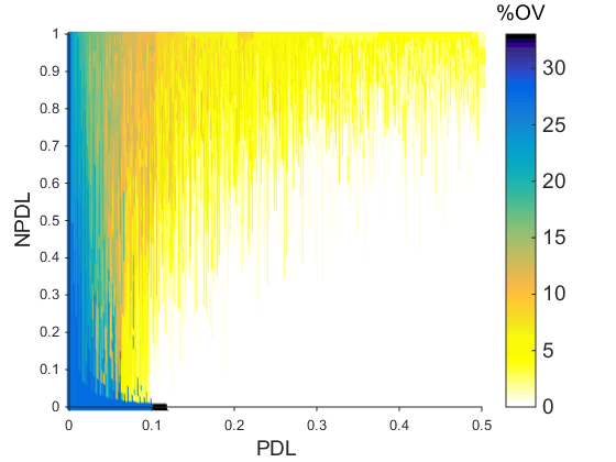
(a) $\%$OV(PCBK)

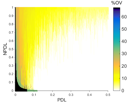
(b) $\%$OV(DARS)

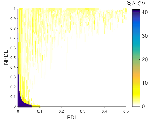
(c) $\%\Delta$OV(DARS,PCBK)

Figure 10: Simulation VI (NPDL vs. PDL).

However, for $NPDl=0.5$, one of the precedence dependencies will change to negative (conflicts-with). As this is performed randomly, we have either (a): $r_{1}$ requires $r_{2}$ AND $r_{2}$ conflicts with $r_{1}$ or (b): $r_{2}$ requires $r_{1}$ AND $r_{1}$ conflicts with $r_{2}$. It is clear that in either case (for Budget $\geq 50$), at least one requirement ($r_{2}$ in (a) and $r_{1}$ in (b)) can be selected. For $\%\text{Budget}=100$, nevertheless, both $r_{1}$ and $r_{2}$ are selected in (a). This, clearly shows how, for a given $PDL$, increasing $NPDL$ can provide higher $\%OV$.

Last but not least, we observed that for simulations with PDL$\geq 0.1$, the performance of PCBK and DARS converged as both methods provided similar $\%OV$: $\Delta\%$OV(DARS,PCBK)$\rightarrow 0$. But this was not the case in the presence of higher levels of negative precedence dependencies. The reason is a large number of precedence dependencies substantially reduces the number of feasible solutions impacting the performance of DARS and PCBK. Nonetheless, increasing NPDL can increase the number of feasible solutions as explained above. Under such circumstances, it is clear that the DARS method can make better choices with regard to the $\%$OV as it takes into account value dependencies in addition to the precedence dependencies.

VI Scalability Analysis

This section evaluates the scalability of DARS for integrating value dependencies in software requirement selection. We generate random datasets with different numbers of requirements to investigate the scalability of the ILP model of DARS (DARS-ILP) for different scenarios in relation to value dependencies as well as precedence dependencies among requirements. Simulations thus were designed to answer the following questions.

• How scalable is DARS-ILP to large requirement sets?

• What is the impact of budget on the runtime of DARS-ILP?

• What is the impact of precedence dependencies on the runtime of DARS-ILP?

• What is the impact of value dependencies on the runtime of DARS-ILP?

The ILP model of DARS, as given by (30)-(38), is scalable to datasets with a large number of requirements, different budget constraints, and various degrees of precedence/value dependencies. To demonstrate this, runtime simulations in Table VI were carried out. To simulate value dependencies for a desired VDL and NVDL, uniformly distributed random numbers in $[-1,1]$ were generated, where the sign and magnitude of each number specified the quality and the strength of its corresponding explicit value dependency. We used PDL and NPDL as given by (53) and (54) to specify the degree of precedence dependencies in a precedence graph of the requirements.

TABLE VI: Runtime simulations

Simulation	Size	$\%$Budget	VDL	NVDL	PDL	NPDL
1	[0,3000]	50	0.15	0.00	0.02	0.00
2	200	[0,100]	0.15	0.00	0.02	0.00
3	200	50	0.15	0	[0,1]	0.00
4	200	50	0.15	0.00	0.02	[0,1]
5	200	50	[0,1]	0.00	0.02	0.00
6	200	50	0.15	[0,1]	0.02	0.00

For a given PDL and NPDL, random numbers in $\{-1,0,1\}$ were generated where $1$ ($-1$) specified a positive (negative) precedence dependency and $0$ denoted the absence of any precedence dependency from a requirement $r_{i}$ to $r_{j}$. Simulations were carried out using the callable library ILOG CPLEX 12.6.2 on a windows machine with a Core i7-2600 3.4 GHz processor and 16 GB of RAM.

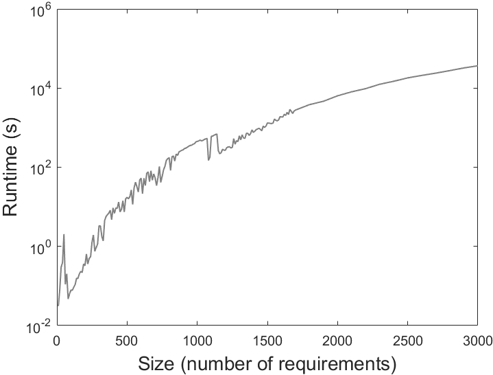
(a) Simulation 1

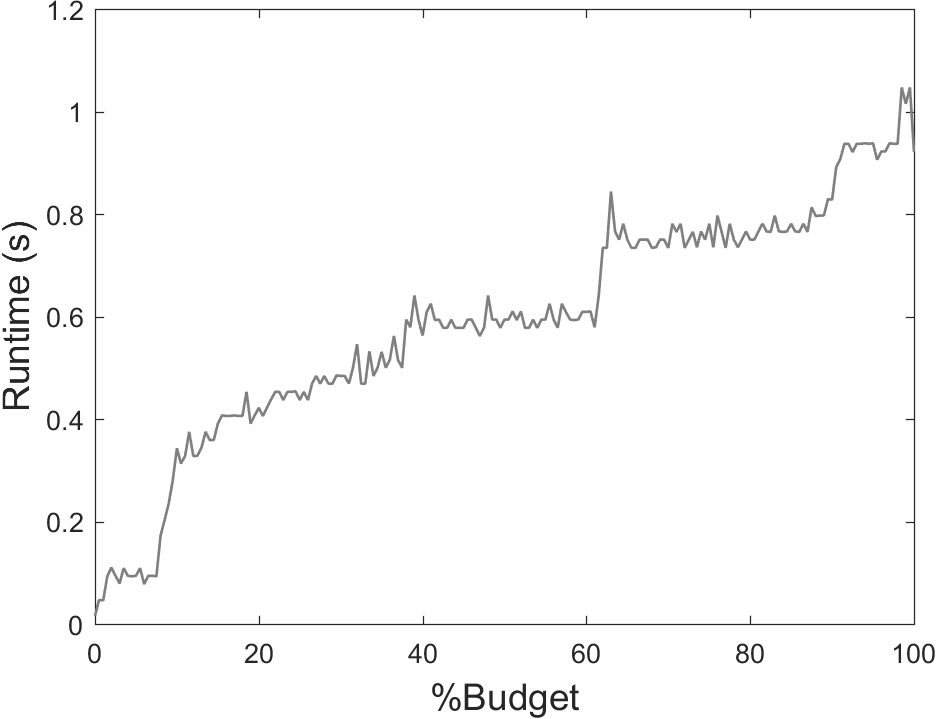
(b) Simulation 2

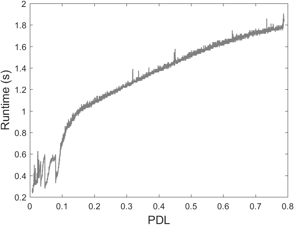
(c) Simulation 3

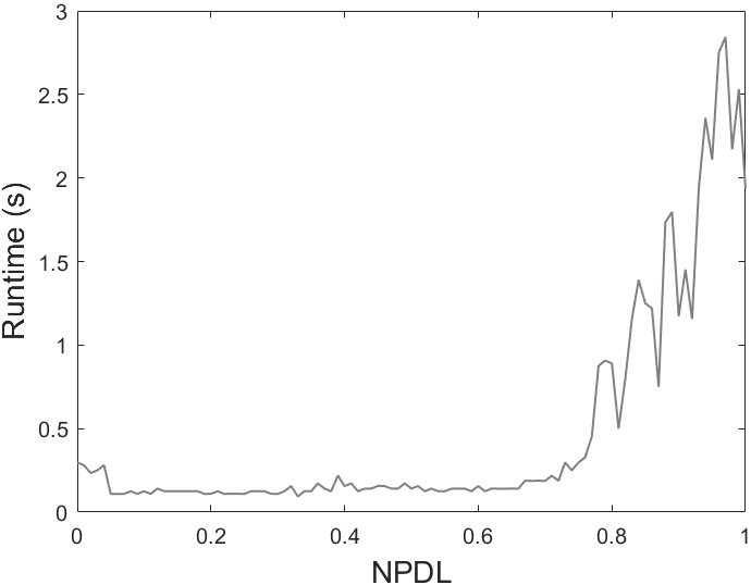
(d) Simulation 4

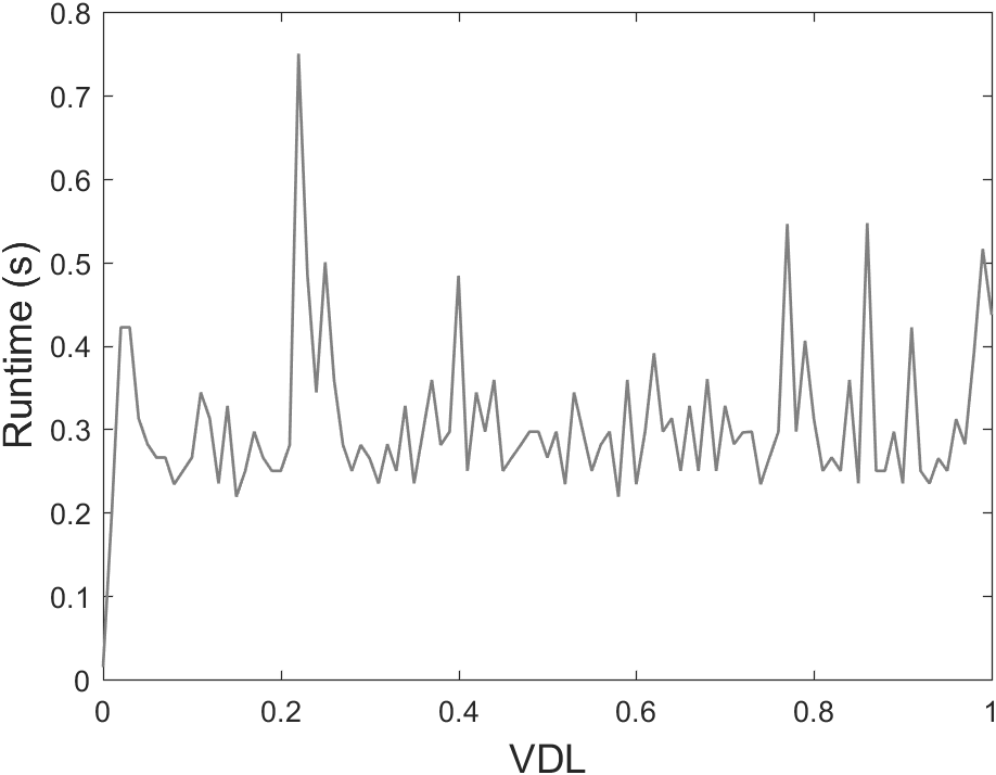
(e) Simulation 5

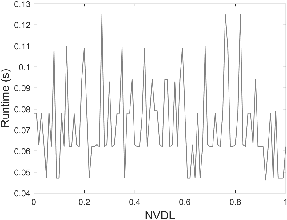
(f) Simulation 6

Figure 11: Runtime of DARS-ILP.

(RQ7) is answered by Simulation 1, which evaluates the runtime of DARS-ILP for different numbers of requirements (Figure 11(a)). We observed that increasing the number of requirements increased the runtime of DARS-ILP. Nonetheless, for requirement sets with up to $750$ requirements ($n\leq 750$), the model managed to find the optimal solution in less than a minute. For $750<n\leq 2000$, the runtime exceeded a minute but did not go beyond two hours. Finally, for $2000<n\leq 3000$ it took few hours before selection was completed. Simulation 2 demonstrated (Figure 11(b)) that the runtime of DARS-ILP increased with budget increase (RQ8). The reason is with more budget, more requirements can be selected, which results in a larger solution space; it may take longer to find the optimal subset.

To answer (RQ9), we simulated requirement selection for various precedence dependency levels (PDLs). Our results (Figure 11(c)) demonstrated that, in general, the runtime of DARS-ILP increased when PDL increased. The reason is increasing PDL limits the number of choices for DARS-ILP as the model needs to respect precedence dependencies; it takes longer for the selection task to complete. Increasing NPDL, on the other hand, had no significant impact on the runtime of DARS-ILP in most places. Nonetheless, for larger NPDLs ($NPDL\rightarrow 1$), runtime was increased. The reason is at such high NPDL, DARS-ILP cannot find a feasible solution with some values due to the high level of conflicts among the requirements.

Simulation 5 and Simulation 6 were carried out to answer (RQ10) by measuring the runtime of the selection models in the presence of various value dependency levels (VDLs) and negative value dependency levels (NVDLs). Our results demonstrate (Figure 11(e)) that increasing (decreasing) VDL has an inconsistent impact of negligible magnitude on the runtime of DARS-ILP. We further, observed (Figure 11(f)) that the impact of increasing (decreasing) NVDL on the runtime of DARS-ILP was unpredictable.

VII Conclusions and Future Work

In this paper, we proposed a fuzzy-based method for integrating value dependencies in software requirement selection. The proposed method, referred to as DARS (Dependency Aware Requirement Selection), uses fuzzy graphs and integer programming to reduce the value loss induced by ignoring value dependencies among software requirements. DARS comprises two major components: (i) a fuzzy-based technique for identifying and modeling value dependencies, and (ii) an integer programming model that explicitly accounts for value dependencies in requirement selection. We have further, proposed a complementary model that can be used to reduce the risk of value loss when quantifying value dependencies is hard. We demonstrated the effectiveness and scalability of DARS by carrying out simulations on the requirements of a real-world software project with results indicative of using DARS reducing value loss. Our results show that (a) compared to existing requirement selection methods, DARS provides higher overall value, (b) maximizing the accumulated value of a requirement subset conflicts with maximizing its overall value – where value dependencies are considered, and (c) DARS is scalable to large requirement sets with different levels of dependencies among requirements.

The work can be extended by exploring techniques for automated collection of user preferences, which serve as the input to the dependency identification process in DARS. Online application stores can be used for this purpose. Moreover, the definition of value can be extended to human values such as fairness and equality, and variations of DARS can be developed to account for such values as well as the dependencies (conflicts) among them in requirement selection.

References

- [1] Y. Zhang, M. Harman, G. Ochoa, G. Ruhe, and S. Brinkkemper, “An empirical study of meta- and hyper-heuristic search for multi-objective release planning,” ACM Trans. Softw. Eng. Methodol., vol. 27, no. 1, pp. 3:1–3:32, Jun. 2018.
- [2] A. J. Bagnall, V. J. RaywardSmith, and I. M. Whittley, “The next release problem,” Information and Software Technology, vol. 43, no. 14, pp. 883–890, Dec. 2001.
- [3] X. Franch and G. Ruhe, “Software release planning,” in Proceedings of the 38th International Conference on Software Engineering Companion. ACM, 2016, pp. 894–895.
- [4] D. Mougouei, D. M. Powers, and E. Mougouei, “A fuzzy framework for prioritization and partial selection of security requirements in software projects,” Journal of Intelligent & Fuzzy Systems, no. Preprint, pp. 2671–2686, 2019.
- [5] D. Mougouei, H. Shen, and A. Babar, “Partial selection of agile software requirements,” International Journal of Software Engineering & Its Applications, vol. 9, no. 1, pp. 113–126, 2015.
- [6] Å. G. Dahlstedt and A. Persson, “Requirements interdependencies: state of the art and future challenges,” in Engineering and managing software requirements. Springer, 2005, pp. 95–116.
- [7] P. Carlshamre, K. Sandahl, M. Lindvall, B. Regnell, and J. Natt och Dag, “An industrial survey of requirements interdependencies in software product release planning,” in Fifth IEEE International Symposium on Requirements Engineering, 2001. Proceedings, 2001, pp. 84–91.
- [8] P. Carlshamre, “Release planning in market-driven software product development: Provoking an understanding,” Requirements Engineering, vol. 7, no. 3, pp. 139–151, Sep. 2002.
- [9] A. M. Pitangueira, R. S. P. Maciel, and M. Barros, “Software requirements selection and prioritization using sbse approaches: A systematic review and mapping of the literature,” Journal of Systems and Software, vol. 103, pp. 267–280, 2015.
- [10] Y. Zhang, M. Harman, and S. L. Lim, “Empirical evaluation of search based requirements interaction management,” Information and Software Technology, vol. 55, no. 1, pp. 126 – 152, 2013, special section: Best papers from the 2nd International Symposium on Search Based Software Engineering 2010.
- [11] W. N. Robinson, S. D. Pawlowski, and V. Volkov, “Requirements interaction management,” ACM Comput. Surv., vol. 35, no. 2, pp. 132-190, Jun. 2003.
- [12] D. Mougouei, “Factoring requirement dependencies in software requirement selection using graphs and integer programming,” in 2016 31st IEEE/ACM International Conference on Automated Software Engineering (ASE). IEEE, 2016, pp. 884–887.
- [13] D. Mougouei, D. M. W. Powers, and A. Moeini, “Dependency-aware software release planning,” in Proceedings of the 39th International Conference on Software Engineering Companion, ser. ICSE-C ’17. IEEE Press, 2017, p. 198–200. [Online]. Available: https://doi.org/10.1109/ICSE-C.2017.74
- [14] D. Mougouei and D. M. Powers, “Modeling and selection of interdependent software requirements using fuzzy graphs,” International Journal of Fuzzy Systems, pp. 1–17, 2017.
- [15] ——, “Dependency-aware release planning for software projects using fuzzy graphs and integer programming,” Journal of Intelligent & Fuzzy Systems, pp. 3693–3707, 2019.
- [16] C. Li, M. v. d. Akker, S. Brinkkemper, and G. Diepen, “An integrated approach for requirement selection and scheduling in software release planning,” Requirements Engineering, vol. 15, no. 4, pp. 375–396, Nov. 2010.
- [17] H. Zhang, J. Li, L. Zhu, R. Jeffery, Y. Liu, Q. Wang, and M. Li, “Investigating dependencies in software requirements for change propagation analysis,” Information and Software Technology, vol. 56, no. 1, pp. 40–53, 2014.
- [18] J. Karlsson, S. Olsson, and K. Ryan, “Improved practical support for largescale requirements prioritising,” Requirements Engineering, vol. 2, no. 1, pp. 51–60, Mar. 1997.
- [19] D. Mougouei and D. M. Powers, “Dependency-aware software release planning through mining user preferences,” Soft Computing, 2020.
- [20] A. Ngo-The and G. Ruhe, “A systematic approach for solving the wicked problem of software release planning,” Soft Computing, vol. 12, no. 1, pp. 95–108, 2008.
- [21] A. Ngo-The and M. O. Saliu, “Measuring dependency constraint satisfaction in software release planning using dissimilarity of fuzzy graphs,” in Cognitive Informatics, 2005.(ICCI 2005). Fourth IEEE Conference on. IEEE, 2005, pp. 301–307.
- [22] J. Wang, J. Li, Q. Wang, H. Zhang, and H. Wang, “A simulation approach for impact analysis of requirement volatility considering dependency change,” in Requirements Engineering: Foundation for Software Quality, B. Regnell and D. Damian, Eds. Springer Berlin Heidelberg, Jan. 2012, no. 7195, pp. 59–76.
- [23] P. Baker, M. Harman, K. Steinhofel, and A. Skaliotis, “Search based approaches to component selection and prioritization for the next release problem,” in Proceedings of the 22Nd IEEE International Conference on Software Maintenance. IEEE, 2006, pp. 176–185.
- [24] M. A. Boschetti, M. Golfarelli, S. Rizzi, and E. Turricchia, “A lagrangian heuristic for sprint planning in agile software development,” Computers & Operations Research, vol. 43, pp. 116–128, Mar. 2014.
- [25] A. A. Araújo, M. Paixao, I. Yeltsin, A. Dantas, and J. Souza, “An architecture based on interactive optimization and machine learning applied to the next release problem,” Automated Software Engineering, pp. 1–49, 2016.
- [26] D. Greer and G. Ruhe, “Software release planning: an evolutionary and iterative approach,” Information and Software Technology, vol. 46, no. 4, pp. 243 – 253, 2004.
- [27] A. Pitangueira, P. Tonella, A. Susi, R. Maciel, and M. Barros, “Minimizing the stakeholder dissatisfaction risk in requirement selection for next release planning,” Information and Software Technology, 2017.
- [28] L. Li, M. Harman, F. Wu, and Y. Zhang, “The value of exact analysis in requirements selection,” IEEE Transactions on Software Engineering, vol. 43, no. 6, pp. 580–596, 2017.
- [29] L. Li, M. Harman, E. Letier, and Y. Zhang, “Robust next release problem: handling uncertainty during optimization,” in Proceedings of the 2014 Annual Conference on Genetic and Evolutionary Computation. ACM, 2014, pp. 1247–1254.
- [30] M. van den Akker, S. Brinkkemper, G. van Diepen, and J. Versendaal, “Flexible release planning using integer linear programming,” REFSQ’05, 2005.
- [31] J. d. Sagrado, I. M. d. Águila, and F. J. Orellana, “Multiobjective ant colony optimization for requirements selection,” Empirical Software Engineering, pp. 1–34, Nov. 2013.
- [32] E. Eells, Probabilistic causality. Cambridge University Press, 1991, vol. 1.
- [33] A. Rosenfeld, “Fuzzy graphs,” Fuzzy Sets and Their Applications, vol. 77, p. 95, 1975.
- [34] A. Kalampakas, S. Spartalis, L. Iliadis, and E. Pimenidis, “Fuzzy graphs: algebraic structure and syntactic recognition,” Artificial Intelligence Review, pp. 1–12, Jul. 2013.
- [35] A. Ngo The and M. O. Saliu, “Fuzzy structural dependency constraints in software release planning,” in The 14th IEEE International Conference on Fuzzy Systems, 2005. FUZZ’05. IEEE, 2005, pp. 442–447.
- [36] X. F. Liu and J. Yen, “An analytic framework for specifying and analyzing imprecise requirements,” in Proceedings of the 18th international conference on Software engineering. IEEE Computer Society, 1996, pp. 60–69.
- [37] D. Mougouei, H. Perera, W. Hussain, R. Shams, and J. Whittle, “Operationalizing human values in software: A research roadmap,” in Proceedings of the 2018 26th ACM Joint Meeting on European Software Engineering Conference and Symposium on the Foundations of Software Engineering, ser. ESEC/FSE 2018. New York, NY, USA: ACM, 2018, pp. 780–784. [Online]. Available: http://doi.acm.org.ezproxy.lib.monash.edu.au/10.1145/3236024.3264843
- [38] H. Perera, A. Nurwidyantoro, W. Hussain, D. Mougouei, J. Whittle, R. A. Shams, and G. Oliver, “A study on the prevalence of human values in software engineering publications, 2015-2018,” arXiv preprint arXiv:1907.07874, 2019.
- [39] H. Perera, W. Hussain, D. Mougouei, R. A. Shams, A. Nurwidyantoro, and J. Whittle, “Towards integrating human values into software: Mapping principles and rights of gdpr to values,” in 2019 IEEE 27th International Requirements Engineering Conference (RE). IEEE, 2019, pp. 404–409.
- [40] W. Hussain, D. Mougouei, and J. Whittle, “Integrating social values into software design patterns,” in 2018 IEEE/ACM International Workshop on Software Fairness (FairWare). IEEE, 2018, pp. 8–14.
- [41] M. M. A. Brasil, T. G. N. d. Silva, F. G. d. Freitas, J. T. d. Souza, and M. I. Cortés, “A multiobjective optimization approach to the software release planning with undefined number of releases and interdependent requirements,” in Enterprise Information Systems, R. Zhang, J. Zhang, Z. Zhang, J. Filipe, and J. Cordeiro, Eds. Springer Berlin Heidelberg, Jan. 2012, no. 102, pp. 300–314.
- [42] J. Karlsson and K. Ryan, “A costvalue approach for prioritizing requirements,” IEEE Software, vol. 14, no. 5, pp. 67–74, Sep. 1997.
- [43] H.-W. Jung, “Optimizing value and cost in requirements analysis,” IEEE Software, vol. 15, no. 4, pp. 74–78, Jul. 1998.
- [44] Y. Zhang, M. Harman, and S. A. Mansouri, “The multi-objective next release problem,” in Proceedings of the 9th Annual Conference on Genetic and Evolutionary Computation. New York, NY, USA: ACM, 2007, p. 1129–1137.
- [45] A. Finkelstein, M. Harman, S. A. Mansouri, J. Ren, and Y. Zhang, “A search based approach to fairness analysis in requirement assignments to aid negotiation, mediation and decision making,” Requirements Engineering, vol. 14, no. 4, pp. 231–245, 2009.
- [46] Y. Zhang, M. Harman, A. Finkelstein, and S. A. Mansouri, “Comparing the performance of metaheuristics for the analysis of multi-stakeholder tradeoffs in requirements optimisation,” Information and Software Technology, vol. 53, no. 7, pp. 761–773, 2011.
- [47] J. del Sagrado, I. M. del Aguila, and F. J. Orellana, “Ant colony optimization for the next release problem: A comparative study,” in Search Based Software Engineering (SSBSE), 2010 Second International Symposium on. IEEE, 2010, pp. 67–76.
- [48] A. C. Kumari, K. Srinivas, and M. Gupta, “Software requirements selection using quantum-inspired elitist multi-objective evolutionary algorithm,” in Advances in Engineering, Science and Management (ICAESM), 2012 International Conference on. IEEE, 2012, pp. 782–787.
- [49] N. Veerapen, G. Ochoa, M. Harman, and E. K. Burke, “An integer linear programming approach to the single and bi-objective next release problem,” Information and Software Technology, vol. 65, pp. 1–13, 2015.
- [50] D. Greer and G. Ruhe, “Software release planning: an evolutionary and iterative approach,” vol. 46, no. 4, pp. 243–253, 2004.
- [51] G. Ruhe and D. Greer, “Quantitative studies in software release planning under risk and resource constraints,” in Proceedings of the 2003 International Symposium on Empirical Software Engineering, Sept 2003, pp. 262–270.
- [52] G. van Valkenhoef, T. Tervonen, B. de Brock, and D. Postmus, “Quantitative release planning in extreme programming,” Information and software technology, vol. 53, no. 11, pp. 1227–1235, 2011.
- [53] Y. Zhang and M. Harman, “Search based optimization of requirements interaction management,” in Search Based Software Engineering (SSBSE), 2010 Second International Symposium on. IEEE, 2010, pp. 47–56.
- [54] P. Tonella, A. Susi, and F. Palma, “Using interactive ga for requirements prioritization,” in Search Based Software Engineering (SSBSE), 2010 Second International Symposium on. IEEE, 2010, pp. 57–66.
- [55] F. G. Freitas, D. P. Coutinho, and J. T. Souza, “Software next release planning approach through exact optimization,” Int. J. Comput. Appl, vol. 22, no. 8, pp. 1–8, 2011.
- [56] F. Colares, J. Souza, R. Carmo, C. Padua, and G. Mateus, “A new approach to the software release planning,” in Software Engineering, 2009. SBES ’09. XXIII Brazilian Symposium on, Oct 2009, pp. 207–215.
- [57] M. O. Saliu and G. Ruhe, “Bi-objective release planning for evolving software systems,” in Proceedings of the the 6th joint meeting of the European software engineering conference and the ACM SIGSOFT symposium on The foundations of software engineering. ACM, 2007, pp. 105–114.
- [58] O. Saliu and G. Ruhe, “Supporting software release planning decisions for evolving systems,” in 29th Annual IEEE/NASA Software Engineering Workshop. IEEE, 2005, pp. 14–26.
- [59] H. Jiang, J. Zhang, J. Xuan, Z. Ren, and Y. Hu, “A hybrid aco algorithm for the next release problem,” in Software Engineering and Data Mining (SEDM), 2010 2nd International Conference on. IEEE, 2010, pp. 166–171.
- [60] M. van den Akker, S. Brinkkemper, G. Diepen, and J. Versendaal, “Determination of the next release of a software product: an approach using integer linear programming.” in CAiSE Short Paper Proceedings, 2005.
- [61] A. Ngo-The and G. Ruhe, “Optimized resource allocation for software release planning,” IEEE Transactions on Software Engineering, vol. 35, no. 1, pp. 109–123, 2009.
- [62] W.-N. Chen and J. Zhang, “Ant colony optimization for software project scheduling and staffing with an event-based scheduler,” IEEE Transactions on Software Engineering, vol. 39, no. 1, pp. 1–17, 2013.
- [63] J. del Sagrado, I. M. ÁAguila, and F. J. Orellana, “Requirements interaction in the next release problem,” in Proceedings of the 13th annual conference companion on Genetic and evolutionary computation. ACM, 2011, pp. 241–242.
- [64] F. Colares, J. Souza, R. Carmo, C. Pádua, and G. R. Mateus, “A new approach to the software release planning,” in Software Engineering, 2009. SBES’09. XXIII Brazilian Symposium on. IEEE, 2009, pp. 207–215.
- [65] A. M. Pitangueira, P. Tonella, A. Susi, R. S. Maciel, and M. Barros, “Risk-aware multi-stakeholder next release planning using multi-objective optimization,” in International Working Conference on Requirements Engineering: Foundation for Software Quality. Springer, 2016, pp. 3–18.
- [66] M. van den Akker, S. Brinkkemper, G. Diepen, and J. Versendaal, “Software product release planning through optimization and what-if analysis,” Information and Software Technology, vol. 50, no. 1, pp. 101–111, 2008.
- [67] P. Tonella, A. Susi, and F. Palma, “Interactive requirements prioritization using a genetic algorithm,” Information and software technology, vol. 55, no. 1, pp. 173–187, 2013.
- [68] J. Xuan, H. Jiang, Z. Ren, and Z. Luo, “Solving the large scale next release problem with a backbone-based multilevel algorithm,” IEEE Transactions on Software Engineering, vol. 38, no. 5, pp. 1195–1212, 2012.
- [69] O. Saliu and G. Ruhe, “Software release planning for evolving systems,” Innovations in Systems and Software Engineering, vol. 1, no. 2, pp. 189–204, 2005.
- [70] M. Harman, J. Krinke, I. MedinaBulo, F. PalomoLozano, J. Ren, and S. Yoo, “Exact scalable sensitivity analysis for the next release problem,” ACM Trans. Softw. Eng. Methodol., vol. 23, no. 2, p. 19:1–19:31, Apr. 2014.
- [71] J. Zhang, Y. Wang, and T. Xie, “Software feature refinement prioritization based on online user review mining,” Information and Software Technology, vol. 108, pp. 30–34, 2019.
- [72] J. Y. Halpern and C. Hitchcock, “Graded causation and defaults,” The British Journal for the Philosophy of Science, vol. 66, no. 2, pp. 413–457, 2015.
- [73] J. Pearl, Causality. Cambridge university press, 2009.
- [74] D. Janzing, D. Balduzzi, M. Grosse-Wentrup, B. Schölkopf et al., “Quantifying causal influences,” The Annals of Statistics, vol. 41, no. 5, pp. 2324–2358, 2013.
- [75] C. W.-K. Leung, S. C.-F. Chan, F.-L. Chung, and G. Ngai, “A probabilistic rating inference framework for mining user preferences from reviews,” World Wide Web, vol. 14, no. 2, pp. 187–215, 2011.
- [76] S. Holland, M. Ester, and W. Kießling, “Preference mining: A novel approach on mining user preferences for personalized applications,” in European Conference on Principles of Data Mining and Knowledge Discovery. Springer, 2003, pp. 204–216.
- [77] A. S. Sayyad, T. Menzies, and H. Ammar, “On the value of user preferences in search-based software engineering: a case study in software product lines,” in 2013 35th International Conference on Software Engineering (ICSE). IEEE, 2013, pp. 492–501.
- [78] L. Villarroel, G. Bavota, B. Russo, R. Oliveto, and M. Di Penta, “Release planning of mobile apps based on user reviews,” in Proceedings of the 38th International Conference on Software Engineering. ACM, 2016, pp. 14–24.
- [79] J. Sprenger, “Foundations for a probabilistic theory of causal strength,” 2016.
- [80] D. Mougouei and W. N. W. A. Rahman, “Fuzzy description of security requirements for intrusion tolerant web-services,” in The Second International Conference on Cyber Security, Cyber Peacefare and Digital Forensic (CyberSec2013). The Society of Digital Information and Wireless Communication, 2013, pp. 141–147.
- [81] D. Mougouei, “Goal-based requirement engineering for fault tolerant security-critical systems,” International Journal of Software Engineering and Its Applications, vol. 7, no. 5, pp. 1–14, 2013.
- [82] S. Mathew and M. Sunitha, “Strongest strong cycles and theta fuzzy graphs,” IEEE Transactions on Fuzzy Systems, vol. 21, no. 6, pp. 1096-1104, Dec 2013.
- [83] D. Mougouei, W. N. W. A. Rahman, and M. Moein Almasi, “Evaluating fault tolerance in security requirements of web services,” in Cyber Security, Cyber Warfare and Digital Forensic (CyberSec), 2012 International Conference on. IEEE, 2012, pp. 111–116.
- [84] D. Mougouei, W. N. W. A. Rahman, and M. M. Almasi, “Measuring security of web services in requirement engineering phase,” International Journal of Cyber-Security and Digital Forensics (IJCSDF), vol. 1, no. 2, pp. 89–98, 2012.
- [85] D. Mougouei, M. Moghtadaei, and S. Moradmand, “A goal-based modeling approach to develop security requirements of fault tolerant security-critical systems,” in Computer and Communication Engineering (ICCCE), 2012 International Conference on. IEEE, 2012, pp. 200–205.
- [86] D. Mougouei, “A mathematical programming approach to considering value dependencies in software requirement selection,” Ph.D. dissertation, Flinders University, School of Computer Science, Engineering and Mathematics., 2018.
- [87] S. Wasserman and K. Faust, Social network analysis: Methods and applications. Cambridge University Press, 1994, vol. 8.
- [88] L. A. Zadeh, “Fyzzy sets,” Inf. Comput., vol. 8, pp. 338-353, Dec 1965.
- [89] J. De Kleer and J. S. Brown, “A qualitative physics based on confluences,” Artificial intelligence, vol. 24, no. 1, pp. 7–83, 1984.
- [90] M. P. Wellman and M. Derthick, Formulation of tradeoffs in planning under uncertainty. Pitman London, 1990.
- [91] A. Kusiak and J. Wang, “Dependency analysis in constraint negotiation,” Systems, Man and Cybernetics, IEEE Transactions on, vol. 25, no. 9, pp. 1301–1313, 1995.
- [92] R. W. Floyd, “Algorithm 97: shortest path,” Communications of the ACM, vol. 5, no. 6, p. 345, 1962.
- [93] S. Boyd and L. Vandenberghe, Convex optimization. Cambridge university press, 2004.
- [94] D. Mougouei, D. M. W. Powers, and A. Moeini, An Integer Linear Programming Model for Binary Knapsack Problem with Dependent Item Values. Cham: Springer International Publishing, 2017, pp. 144–154. [Online]. Available: https://doi.org/10.1007/978-3-319-63004-5_12
- [95] D. G. Luenberger and Y. Ye, Linear and nonlinear programming. Springer, 2015, vol. 228.
- [96] R. T. Marler and J. S. Arora, “Survey of multi-objective optimization methods for engineering,” Structural and multidisciplinary optimization, vol. 26, no. 6, pp. 369–395, 2004.
- [97] I. I. CPLEX, “V12.7: Cplex user’s manual,” International Business Machines Corporation, 2016.