Estimating multi-index models
with response-conditional least squares

Abstract

The multi-index model is a simple yet powerful high-dimensional regression model which circumvents the curse of dimensionality assuming $\mathbb{E}[Y|X]=g(A^{\top}X)$ for some unknown index space $A$ and link function $g$. In this paper we introduce a method for the estimation of the index space, and study the propagation error of an index space estimate in the regression of the link function. The proposed method approximates the index space by the span of linear regression slope coefficients computed over level sets of the data. Being based on ordinary least squares, our approach is easy to implement and computationally efficient. We prove a tight concentration bound that shows $N^{-1/2}$-convergence, but also faithfully describes the dependence on the chosen partition of level sets, hence giving indications on the hyperparameter tuning. The estimator’s competitiveness is confirmed by extensive comparisons with state-of-the-art methods, both on synthetic and real data sets. As a second contribution, we establish minimax optimal generalization bounds for k-nearest neighbors and piecewise polynomial regression when trained on samples projected onto any $N^{-1/2}$-consistent estimate of the index space, thus providing complete and provable estimation of the multi-index model.

, and

1 Introduction

Many recent advances in the analysis of high-dimensional data are based on the observation that real-world data are inherently structured, and the relationship between variables, features and responses is often of a lower dimensional nature [1, 5, 28, 29, 39, 40]. A popular model incorporating this structural assumption is the multi-index model, which poses the relation between a predictor $X\in\mathbb{R}^{D}$ and a response $Y\in\mathbb{R}$ as

$$Y=g(A^{\top}X)+\zeta,$$ (1)

where $A\in\mathbb{R}^{D\times d}$ is an unknown full column rank matrix with $d\ll D$, $g:\mathbb{R}^{d}\to\mathbb{R}$ is an unknown function, and $\zeta$ is a noise term with $\mathbb{E}[\zeta|X]=0$, independent of $X$ given $A^{\top}X$. In the following we refer to $g$ as the link function and $A$ as the index space, assuming, without loss of generality, that the columns of $A$ are orthonormal [13]. Model (1) asserts that the information required to predict the conditional expectation $f(x):=\mathbb{E}[Y|X=x]$ is encoded in the distribution of $A^{\top}X$. Therefore, knowing the projection $P:=AA^{\top}$ allows to estimate $f$ in a nonparametric fashion with a number of samples scaling with the intrinsic dimension $d$, rather than the ambient dimension $D$.

Ways to estimate the index space have been studied extensively over the years and by now several methods have been proposed. Most of them originate from the statistical literature, starting with the seminal work of [36] and going forward with [9, 34, 35]. In recent years, the problem has gained popularity also in the machine learning community, due to its relation and similarity to (shallow) neural networks [13, 14, 19]. Despite the variety of available approaches, there is no distinctly best method: some estimators are better suited for practical purposes as they are computationally efficient and easy to implement, while others generally enjoy better theoretical guarantees. We provide an extensive overview in Section 1.1.

In this work we derive and analyze a method for estimating $f$ under the model assumption (1) from a given data set $\{(X_{i},Y_{i}):i=1,\dots,N\}$, where $(X_{i},Y_{i})$ are independent copies of $(X,Y)$. First, we construct an estimate $\hat{P}$ of the projection $P$ based on the span of response-conditional least-squares vectors of the data. Once $\hat{P}$ has been computed, the second step is a regression task on the reduced data set $\{(\hat{P}X_{i},Y_{i}):i=1,\dots,N\}$, which can be solved by classical nonparametric estimators such as piecewise polynomials or kNN-regression. The proposed method is attractive for practitioners due to its simplicity and efficiency, with almost no parameter adjustment needed. Furthermore, it is provable, with strong theoretical guarantees neatly derivable from a few reasonable assumptions. We establish tight concentration bounds describing the estimator’s performance in the finite sample regime. In particular, we prove that $\|\hat{P}-P\|\in{\cal O}(N^{-1/2})$, and determine the explicit dependence of the constants on the parameters involved. A data-driven approximation of the index space error empirically confirms the tightness of our concentration bound, providing guidance for hyperparameter tuning. Moreover, to the best of our knowledge, we are the first ones to provide generalization guarantees for model (1) that take into account the propagation of the projection error $\|\hat{P}-P\|$ into the reduced regression problem. Specifically, we analyze two popular regression methods, namely k-nearest neighbors regression (kNN) and piecewise polynomial regression, and show that the minimax optimal $d$-dimensional estimation rate is achieved if $\hat{P}$ is any index estimate such that $\|\hat{P}-P\|\in{\cal O}(N^{-1/2})$.

1.1 Related work on index space estimation

Many methods for estimating the index space have been developed in the statistical literature under the name of sufficient dimension reduction [33], where the multi-index model is relaxed to

$$Y\mathchoice{\mathrel{\hbox to0.0pt{$\displaystyle\perp$\hss}\mkern 2.0mu{\displaystyle\perp}}}{\mathrel{\hbox to0.0pt{$\textstyle\perp$\hss}\mkern 2.0mu{\textstyle\perp}}}{\mathrel{\hbox to0.0pt{$\scriptstyle\perp$\hss}\mkern 2.0mu{\scriptstyle\perp}}}{\mathrel{\hbox to0.0pt{$\scriptscriptstyle\perp$\hss}\mkern 2.0mu{\scriptscriptstyle\perp}}}X|A^{\top}X.$$ (2)

Note that this setting generalizes our problem since (1) and $\varepsilon\mathchoice{\mathrel{\hbox to0.0pt{$\displaystyle\perp$\hss}\mkern 2.0mu{\displaystyle\perp}}}{\mathrel{\hbox to0.0pt{$\textstyle\perp$\hss}\mkern 2.0mu{\textstyle\perp}}}{\mathrel{\hbox to0.0pt{$\scriptstyle\perp$\hss}\mkern 2.0mu{\scriptstyle\perp}}}{\mathrel{\hbox to0.0pt{$\scriptscriptstyle\perp$\hss}\mkern 2.0mu{\scriptscriptstyle\perp}}}X|A^{\top}X$ imply (2). A space $\operatorname{Im}(A)$ satisfying (2) is called a dimension reduction subspace, and if the intersection of such spaces satisfies (2) it is called central subspace. Except for degenerate cases, a unique central subspace exists [7, 8]. One can also consider a model where (2) is replaced by $Y\mathchoice{\mathrel{\hbox to0.0pt{$\displaystyle\perp$\hss}\mkern 2.0mu{\displaystyle\perp}}}{\mathrel{\hbox to0.0pt{$\textstyle\perp$\hss}\mkern 2.0mu{\textstyle\perp}}}{\mathrel{\hbox to0.0pt{$\scriptstyle\perp$\hss}\mkern 2.0mu{\scriptstyle\perp}}}{\mathrel{\hbox to0.0pt{$\scriptscriptstyle\perp$\hss}\mkern 2.0mu{\scriptscriptstyle\perp}}}\mathbb{E}[Y|X]|A^{\top}X$, which leads to the definition of central mean subspace [10]. In the case of model (1) with $\varepsilon\mathchoice{\mathrel{\hbox to0.0pt{$\displaystyle\perp$\hss}\mkern 2.0mu{\displaystyle\perp}}}{\mathrel{\hbox to0.0pt{$\textstyle\perp$\hss}\mkern 2.0mu{\textstyle\perp}}}{\mathrel{\hbox to0.0pt{$\scriptstyle\perp$\hss}\mkern 2.0mu{\scriptstyle\perp}}}{\mathrel{\hbox to0.0pt{$\scriptscriptstyle\perp$\hss}\mkern 2.0mu{\scriptscriptstyle\perp}}}X|A^{\top}X$, the space $\operatorname{Im}(A)$ is both the central subspace and the central mean subspace [10]. Thus, we will treat related research under the same umbrella.

The methods for sufficient dimension reduction can broadly be grouped into inverse regression based methods and nonparametric methods [1, 42]. The first group reverses the regression dependency between $X$ and $Y$ and uses inverse statistical moments to construct a matrix $\Lambda$ with $\operatorname{Im}(\Lambda)\subseteq\operatorname{Im}(A)$. The most prominent representatives are sliced inverse regression (SIR/SIRII) [36, 37], sliced average variance estimation (SAVE) [9], and contour regression/directional regression (CR/DR) [34, 35] (see Table 1 for the corresponding definition of $\Lambda$). Linear combinations of related matrices $\Lambda$ have been called hybrid methods [54]. Furthermore, in the case where $X$ follows a normal distribution, two popular methods are principal Hessian directions (pHd) [38] and iterative Hessian transformations (iHt) [10]. In this setting, $\Lambda$ is the averaged Hessian matrix of the regression function, which can be efficiently computed using Stein’s Lemma.

If $\operatorname{Im}(\Lambda)\subseteq\operatorname{Im}(A)$, eigenvectors corresponding to nonzero eigenvalues of $\Lambda$ yield an unbiased subspace of the index space $\operatorname{Im}(A)$. A typical assumption to guarantee this is the linear conditional mean (LCM), given by $\mathbb{E}[X|PX]=PX$. It holds, for example, for all elliptically symmetric distributions [36, 42]. Methods based on second order moments usually need in addition the constant conditional variance assumption (CCV), which requires $\operatorname{Cov}\left({X|PX}\right)$ to be nonrandom. In particular, the normal distribution satisfies both LCM and CCV. If $\operatorname{Im}(\Lambda)=\operatorname{Im}(A),$ a method is called exhaustive. A condition to ensure exhaustiveness is $\mathbb{E}[v^{\top}Z|Y]$ being non-degenerate (i.e. not almost surely equal to a constant) for all nonzero $v\in\operatorname{Im}(A)$, where $Z$ is the standardization of $X$. In Table 1 we denote this condition by RCP (random conditional projection), and by RCP² when $\mathbb{E}[v^{\top}Z|Y]$ is replaced by $\mathbb{E}[(v^{\top}Z)^{2}|Y]$.

Method	Matrix $\Lambda$	$\operatorname{Im}(\Lambda)\subseteq\operatorname{Im}(A)$	$\operatorname{Im}(\Lambda)=\operatorname{Im}(A)$
SIR [36]	$\operatorname{Cov}\left({\mathbb{E}[Z|Y]}\right)$	LCM	RCP
SIRII [37]	$\mathbb{E}(\operatorname{Cov}\left({Z|Y}\right)-\mathbb{E}\operatorname{Cov}\left({Z|Y}\right))^{2}$	LCM and CCV	N/A
SAVE  [9]	$\mathbb{E}(\mathsf{Id}-\operatorname{Cov}\left({Z|Y}\right))^{2}$	LCM and CCV	RCP or RCP2
DR [34]	$\mathbb{E}(2\mathsf{Id}-\operatorname{Cov}\left({Z-Z^{\prime})|Y,Y^{\prime}}\right))^{2}$	LCM and CCV	RCP or RCP2
pHd [38]	$\mathbb{E}(Y-\mathbb{E}Y)(X-\mathbb{E}X)(X-\mathbb{E}X)^{\top}$	normal $X$	N/A

Table 1: A summary of prominent inverse regression based methods (plus pHd). We let $Z$ be the standardized $X$, and $(Z^{\prime},Y^{\prime})$ an independent copy of $(Z,Y)$. The table omits details on contour regression [35] (strongly related to DR), iterative Hessian transformations [10] (related to pHd), and hybrid approaches [54] (linear combinations of methods above).

As inverse regression based methods require only computation of finite sample means and covariances, they are efficient and easy to implement. The matrix $\Lambda$ is usually approximated by partitioning the range $\operatorname{Im}(Y)=\cup_{\ell=1}^{J}{\cal R}_{J,\ell}$, and approximating statistics of $X|Y$ by empirical quantized statistics of $X|Y\in{\cal R}_{J,\ell}$. Therefore, only a single hyperparameter, the number of subsets $J$, needs to be tuned. A strategy for choosing $J$ optimally is not known [42].

Nonparametric methods try to estimate the gradient field of the regression function $f$ based on the observation that the $d$ leading eigenvectors of $\mathbb{E}[\nabla f(X)\nabla f(X)^{\top}]$ (assuming $f$ is differentiable) span the index space. The concrete implementation of this idea differs between methods. Popular examples are minimum average variance estimation (MAVE), outer product of gradient estimation (OPG), and variants thereof [53]. While MAVE converges to the index space under mild assumptions, it suffers from the curse of dimensionality due to nonparametric estimation of gradients of $f$. The inverse MAVE (IMAVE) [53] combines MAVE with inverse regression, achieving $N^{-1/2}$-consistency under LCM. Sliced regression [51] collects local MAVE estimates on response slices, producing $N^{-1/2}$-consistent index estimates free of LCM for $d\leq 3$. Furthermore, iterative generalizations of the average derivative estimation (ADE) [18] have been proved to be $N^{-1/2}$-consistent for $d\leq 3$ and $d\leq 4$ [12, 20].

Compared to inverse regression methods, nonparametric methods rely on less stringent assumptions, but are computationally more demanding, require more hyperparameter tuning, and are often more complex to analyze. The relation between inverse regression and nonparametric methods has been investigated in [41, 43] by introducing semiparametric methods. The authors showed that the computational efficiency and simplicity of inverse regression methods come at the cost of assumptions such as LCM/CCV. Moreover, they demonstrated that inverse regression methods can be modified by including a nonparametric estimation step to achieve theoretical guarantees even when LCM/CCV do not hold.

The work presented above originates from statistical literature, and, to the best of our knowledge, focuses only on the index space estimation, completely omitting the subsequent regression step. This is different in the machine learning community, where estimation of both $A$ and $f$ has been recently studied for the case $d=1$ [15, 22, 23, 26, 30, 31, 46]. The problem was also considered for $d\geq 1$ in an active sampling setting, where the user is allowed to query data points $(X,Y)$ and the goal is to minimize the number of queries [13, 19]. Moreover, model (1) has strong ties with shallow neural network models $f(x)=\sum_{i=1}^{m}g_{i}(a_{i}^{\top}x)$, which are currently actively investigated [14, 21, 45, 48].

1.2 Content and contributions of this work

Index space estimation

We propose to estimate the index space by the span of ordinary least squares solutions computed over level sets of the data (see Section 2 for details). We call our method response-conditional least squares (RCLS). Our approach shares typical benefits of inverse regression based techniques: it is computationally efficient, and easy to implement, as only a single hyperparameter (number of level sets) needs to be specified. An additional advantage is that ordinary least squares can be readily exchanged by variants leveraging priors such as sparsity [32, 47] and further.

On the density level, we guarantee that RCLS finds a subspace $\operatorname{Im}(P_{J})$ of $\operatorname{Im}(P)$ under the LCM assumption. In the finite sample regime, we prove a concentration bound

$$\left\|{\hat{P}_{{J}}-P_{J}}\right\|_{F}\lesssim C(J)\sqrt{\frac{D}{N}},$$ (3)

disentangling the influence of the number of samples $N$ and the number of level sets $J$ on the performance of our estimator (Corollary 8). Moreover, we show empirically that $C(J)$ in (3) tightly characterizes the influence of the hyperparameter on the estimator’s performance, providing guidance to how to choose it in practice.

Link function regression

We analyze the performance of kNN regression and piecewise polynomial regression (with respect to a dyadic partition), when trained on the perturbed data set $\{(\hat{P}X_{i},Y_{i}):i=1,\dots,N\}$ instead of $\{(PX_{i},Y_{i}):i=1,\dots,N\}$, where $\hat{P}$ is any estimate of the index projection $P$. Specifically, we prove for sub-Gaussian $X$, $(L,s)$-smooth $g$ (see Definition 9), and almost surely bounded $f(X)$, that the estimator $\hat{f}$ satisfies the generalization bound (Theorems 10 and 13)

$$\mathbb{E}\left(\hat{f}(X)-f(X)\right)^{2}\lesssim N^{-\frac{2s}{2s+d}}+\left\|{\hat{P}-P}\right\|^{\min\{2s,2\}},$$ (4)

where $s\in(0,1]$ in the case of kNN, and $s\in(0,+\infty)$ in the case of piecewise polynomials. The bound (4) shows that optimal estimation rates (in the minimax sense) are achieved by traditional regressors for $d=1$ and $s>\frac{1}{2}$, or $d\geq 2$ and any $s>0$, provided $\|\hat{P}-P\|\in{\cal O}(N^{-1/2})$. In particular, combining (3) and (4) we obtain that RCLS paired with piecewise polynomial regression produces an optimal estimation of the multi-index model.

1.3 Organization of the paper

Section 2 describes RCLS for index space estimation. Section 3 presents theoretical guarantees on the population level and in the finite sample regime. Section 4 establishes the generalization bound (4). Section 5 compares RCLS with state-of-the-art methods on synthetic and real data sets.

1.4 General notation

We let $\mathbb{N}_{0}$ be the set of natural numbers including $0$, and $[J]:=\{1,\ldots,J\}$. We write $a\vee b:=\max\{a,b\}$ and $a\wedge b:=\min\{a,b\}$. Throughout the paper, $C$ stands for a universal constant that may change on each appearance. We use $\|\cdot\|$ for the Euclidean norm of vectors, and $\left\|{\cdot}\right\|$, $\left\|{\cdot}\right\|_{F}$ for the spectral and Frobenius matrix norms, respectively. For a symmetric real matrix $A\in\mathbb{R}^{D\times D}$, we denote the ordered eigenvalues as $\lambda_{1}(A)\geq\cdots\geq\lambda_{D}(A)$ and the corresponding eigenvectors as $u_{1}(A),\dots,u_{D}(A)$.

We denote expectation and covariance of a random vector $X$ by $\mathbb{E}[X]$ and $\operatorname{Cov}\left({X}\right)$, respectively, and let $\tilde{X}:=X-\mathbb{E}[X]$. The sub-Gaussian norm of a random variable $Z$ is $\left\|{Z}\right\|_{\psi_{2}}:=\inf\{t>0:\mathbb{E}\exp(Z^{2}/t^{2})\leq 2\}$. Similarly, the sub-Exponential norm is $\left\|{Z}\right\|_{\psi_{1}}=\inf\{t>0:\mathbb{E}\exp(\left|{Z}\right|/t)\leq 2\}$. Finally, we abbreviate the mean squared error of an estimator $\smash{\hat{f}}$ of $f$ by $\textrm{MSE}(\smash{\hat{f}},f):=\mathbb{E}|\smash{\hat{f}(X)}-f(X)|^{2}$.

2 Index space estimation by response-conditional least squares

Algorithm 1 Index space estimation via RCLS

0:  Parameters $J$ and $\tilde{d}$, data set $\{(X_{i},Y_{i}):i\in[N]\}$

  Split data into $\{{\cal X}_{J,\ell}:\ell\in[J]\}$ and $\{{\cal Y}_{J,\ell}:\ell\in[J]\}$ according to (5)

  for $\ell=1,\ldots,J$ do

     $\hat{b}_{J,\ell}:=\hat{\Sigma}_{J,\ell}^{\dagger}\,\hat{\mathbb{E}}_{({\cal X}_{J,\ell},{\cal Y}_{J,\ell})}{(X-\hat{\mathbb{E}}_{{\cal X}_{J,\ell}}{X})(Y-\hat{\mathbb{E}}_{{\cal Y}_{J,\ell}}{Y})}$

     $\hat{\rho}_{J,\ell}:=\left|{{\cal X}_{J,\ell}}\right|N^{-1}$

  end for

  $\hat{M}_{J}:=\sum_{\ell=1}^{J}\hat{\rho}_{J,\ell}\hat{b}_{J,\ell}\hat{b}_{J,\ell}^{\top}$

  $\hat{P}_{{J}}(\tilde{d})$, the orthoprojector onto the leading $\tilde{d}$ eigenvectors of $\hat{M}_{J}$

We first describe response-conditional least squares (RCLS) and then highlight advantages and disadvantages of the approach compared to other methods in the literature (see Section 1.1).

RCLS

For the sake of simplicity we assume here that $\operatorname{Im}(Y)$ is bounded. First, let $\operatorname{Im}(Y)=\cup_{\ell=1}^{J}{\cal R}_{J,\ell}$ be a dyadic decomposition of the range into $J$ intervals. For example, this means ${\cal R}_{J,\ell}:=[\frac{\ell-1}{J},\frac{\ell}{J})$ in the case $\operatorname{Im}(Y)=[0,1)$. We assign the samples $\{(X_{i},Y_{i}):i\in[N]\}$ to subsets

$${\cal Y}_{J,\ell}:=\{Y_{i}:Y_{i}\in{\cal R}_{J,\ell}\},\quad\textrm{and}\quad{\cal X}_{J,\ell}:=\{X_{i}:Y_{i}\in{\cal R}_{J,\ell}\},$$ (5)

which we refer to as level sets in the following. On each level set we solve an ordinary least squares problem. That is, for the empirical conditional covariance matrix $\hat{\Sigma}_{J,\ell}:=\hat{\mathbb{E}}_{{\cal X}_{j}}{(}X-\hat{\mathbb{E}}_{{\cal X}_{J,\ell}}{X})(X-\hat{\mathbb{E}}_{{\cal X}_{J,\ell}}{X})^{\top}$, where $\hat{\mathbb{E}}_{{\cal X}_{J,\ell}}{X}$ is the usual finite sample mean of $X$ over ${\cal X}_{J,\ell}$, we compute vectors

$$\hat{b}_{J,\ell}:=\hat{\Sigma}_{J,\ell}^{\dagger}\hat{\mathbb{E}}_{({\cal X}_{J,\ell},{\cal Y}_{J,\ell})}{(X-\hat{\mathbb{E}}_{{\cal X}_{J,\ell}}{X})(Y-\hat{\mathbb{E}}_{{\cal Y}_{J\ell}}{Y}}).$$ (6)

Intuitively speaking, $\hat{b}_{J,\ell}$ can be seen as an estimate of the averaged gradient of the regression function $f$ over the level set ${\cal R}_{J,\ell}$. Taking into account the model $f(x)=g(A^{\top}x)$, $\hat{b}_{J,\ell}$ should therefore become increasingly close to the index space $\operatorname{Im}(A)$ as the number of samples in ${\cal X}_{J,\ell}$ increases. This motivates to approximate the index space by the leading eigenvectors of an outer product matrix of vectors $\{\hat{b}_{J,\ell}:\ell\in[J]\}$. We set $\hat{\rho}_{J,\ell}:=\left|{{\cal X}_{J,\ell}}\right|N^{-1}$ and then compute

$$\hat{P}_{{J}}(\tilde{d}):=\sum\limits_{i=1}^{\tilde{d}}u_{i}(\hat{M}_{J})u_{i}(\hat{M}_{J})^{\top},\quad\textrm{where}\quad\hat{M}_{J}:=\sum_{\ell=1}^{J}\hat{\rho}_{J,\ell}\hat{b}_{J,\ell}\hat{b}_{J,\ell}^{\top}.$$ (7)

The parameter $\tilde{d}\leq d$ is user-specified and ideally equals $\dim(\operatorname{span}\{\hat{b}_{J,\ell}:\ell\in[J]\})$ in the limit $N\rightarrow\infty$. If this value is unknown, we select it via model selection techniques or by inspecting the spectrum of $\hat{M}_{J}$. The procedure is summarized in Algorithm 1.

Remark 1 (Choice of partition).

One possible way to decompose $\operatorname{Im}(Y)$ is by dyadic cells. However, the analysis in Section 3 does not require the dyadic structure and can instead be conducted with arbitrary partitions.

Remark 2 (Algorithmic complexity).

The main computational demand is constructing the vectors $\{\hat{b}_{J,\ell}:\ell\in[J]\}$. Assuming we use a partition of disjoint level sets ${\cal R}_{J,\ell}$, i.e. each sample is only used once in the construction of $\hat{M}_{J}$, the cost for this is ${\cal O}(\sum_{\ell=1}^{J}\left|{{\cal X}_{J,\ell}}\right|D^{2})={\cal O}(ND^{2})$.

Comparison of RCLS with inverse regression methods

In RCLS, response conditioning serves to localize and produce multiple estimates rather than induce isotropy in the marginal distribution (e.g. no conditioning is required in the single-index case); hence, it is not a typical inverse regression method. At the same time, it shares the same general advantages: it is simple, computationally efficient, and provable. While in inverse regression no optimal slicing procedure is known, RCLS admits a tight parameter characterization which allows for a straight optimization. On par with all inverse regression methods, RCLS requires the LCM assumption. Although it is often more or at least as accurate as second order inverse regression methods, such as CR and DR, it does not need the CCV assumption. This is a major generalization since, as pointed out in [42], assuming both LCM and CCV for all directions reduces $X$ to the normal distribution. RCLS low computational cost matches that of typical inverse regression estimates (except CR, which is ${\cal O}(N^{2}D^{2})$).

Comparison of RCLS with nonparametric methods

Essentially relying on gradient field estimation, RCLS has strong ties with nonparametric methods, but it has lower computation cost and it is easier to implement. Note that nonparametric methods typically involve kernel smoothing, leading to complexities quadratic in the sample size $N$. Such costs are linearizable resorting for example to nearest neighbor truncation, but while naive kNN still requires the computation of ${\cal O}(N^{2})$ distances, hierarchical structures for fast neighbor search, such as k-d and cover trees [2, 3], imply constants exponential in the dimension $D$, not to mention the overhead resulting from cross-validating the number of neighbors. Cross-validation is in principle also required for bandwidth selection, even for joint tuning of two different bandwidths [51], since optimal choices beyond rules of thumb (e.g. the “normal reference”) are to date an open problem. Last but not least, kernel estimates are sensitive to the curse of dimensionality, whose overcoming requires further complications, algorithmic tweaks, initializations and iterative procedures [51, 53].

3 Guarantees for RCLS

We introduce population counterparts of $\hat{b}_{J,\ell}$ and $\hat{M}_{J}$ given by

$$b_{J,\ell}:=\Sigma_{J,\ell}^{\dagger}\operatorname{Cov}\left({X,Y|Y\in{\cal R}_{J,\ell}}\right)\quad\textrm{ and }\quad M_{J}:=\sum_{\ell=1}^{J}\rho_{J,\ell}b_{J,\ell}b_{J,\ell}^{\top},$$

where $\Sigma_{J,\ell}:=\operatorname{Cov}\left({X|Y\in{\cal R}_{J,l}}\right)$, and $\rho_{J,\ell}:=\mathbb{P}(Y\in{\cal R}_{J,\ell})$. All quantities thus far are defined through the random vector $(X,Y)$ without using the regression function. In fact, in this section we can technically avoid specifying the regression function by assuming a more general setting, where $\operatorname{Im}(P)$ is defined as the minimal dimensional subspace with

1. $Y\mathchoice{\mathrel{\hbox to0.0pt{$\displaystyle\perp$\hss}\mkern 2.0mu{\displaystyle\perp}}}{\mathrel{\hbox to0.0pt{$\textstyle\perp$\hss}\mkern 2.0mu{\textstyle\perp}}}{\mathrel{\hbox to0.0pt{$\scriptstyle\perp$\hss}\mkern 2.0mu{\scriptstyle\perp}}}{\mathrel{\hbox to0.0pt{$\scriptscriptstyle\perp$\hss}\mkern 2.0mu{\scriptscriptstyle\perp}}}X|PX$.

As mentioned in Section 1.1, (A1) uniquely defines $\operatorname{Im}(P)$ except for degenerate cases, which we exclude here. Moreover, (A1) with $P=AA^{\top}$ generalizes (1) and $\zeta\mathchoice{\mathrel{\hbox to0.0pt{$\displaystyle\perp$\hss}\mkern 2.0mu{\displaystyle\perp}}}{\mathrel{\hbox to0.0pt{$\textstyle\perp$\hss}\mkern 2.0mu{\textstyle\perp}}}{\mathrel{\hbox to0.0pt{$\scriptstyle\perp$\hss}\mkern 2.0mu{\scriptstyle\perp}}}{\mathrel{\hbox to0.0pt{$\scriptscriptstyle\perp$\hss}\mkern 2.0mu{\scriptscriptstyle\perp}}}X|A^{\top}X$.

In the following analysis, we also require the following assumptions.

1. $\mathbb{E}[X|PX]=PX$ almost surely;

2. $X$ and $Y$ are sub-Gaussian random variables.

(A2) is the LCM assumption introduced in Section 1.1 and is required in all inverse regression based techniques like SIR, SAVE or DR. It is satisfied for example for any elliptical distribution and ensures $\operatorname{Im}(M_{J})\subseteq\operatorname{Im}(A)$ as shown in Proposition 3 below. (A3) is maximally general to use the tools developed in the framework of sub-Gaussian random variables, namely finite sample concentration bounds. Examples of sub-Gaussian random variables include bounded distributions, the normal distribution, or more generally random variables for which all one-dimensional marginals have tails that exhibit a Gaussian-like decay after a certain threshold [50].

3.1 Population level

The population level results are summarized in the following proposition.

Proposition 3.

If $(X,Y)$ satisfies (A1) and (A2), then $b_{J,\ell}\in\operatorname{Im}(A)$ for any $\ell\in[J]$ and any $J$. Also, $\operatorname{Im}(M_{J})\subseteq\operatorname{Im}(A)$, with equality if $\lambda_{d}\left(M_{J}\right)>0$.

We need the following result for the proof of Proposition 3.

Lemma 4.

Under (A1) and (A2), we get

1. $\mathbb{E}[X|Y]=\mathbb{E}[PX|Y]$ almost surely, or equivalently $\mathbb{E}[QX|Y]=0$;

2. $\operatorname{Cov}\left({X\mid Y}\right)=\operatorname{Cov}\left({PX\mid Y}\right)+\operatorname{Cov}\left({QX\mid Y}\right)$ almost surely.

Proof.

(a). The towering property of conditional expectations yields $\mathbb{E}[X|Y]=\mathbb{E}[\mathbb{E}[X|PX,Y]|Y]$. Assumption (A1) implies $Y\mathchoice{\mathrel{\hbox to0.0pt{$\displaystyle\perp$\hss}\mkern 2.0mu{\displaystyle\perp}}}{\mathrel{\hbox to0.0pt{$\textstyle\perp$\hss}\mkern 2.0mu{\textstyle\perp}}}{\mathrel{\hbox to0.0pt{$\scriptstyle\perp$\hss}\mkern 2.0mu{\scriptstyle\perp}}}{\mathrel{\hbox to0.0pt{$\scriptscriptstyle\perp$\hss}\mkern 2.0mu{\scriptscriptstyle\perp}}}X|PX$, and thus $\mathbb{E}[X|PX,Y]=\mathbb{E}[X|PX]=PX$ by assumption (A2).

(b). By the law of total covariance,

$$\operatorname{Cov}\left({PX,QX|Y}\right) =\mathbb{E}[\operatorname{Cov}\left({PX,QX|PX,Y}\right)|Y]$$

$$+\operatorname{Cov}\left({\mathbb{E}[QX|PX,Y],\mathbb{E}[PX|PX,Y]|Y}\right)=0+0,$$

where we used $\mathbb{E}[X|PX,Y]=PX$ as shown in the proof of (a). Therefore,

$$\operatorname{Cov}\left({X\mid Y}\right)=\operatorname{Cov}\left({PX+QX\mid Y}\right)=\operatorname{Cov}\left({PX\mid Y}\right)+\operatorname{Cov}\left({QX\mid Y}\right).\qed$$

Proof of Proposition 3.

We only show that $b_{J,\ell}\in\operatorname{Im}(A)$ for all $R_{J,\ell}$, since $\operatorname{Im}(M_{J})\subseteq\operatorname{Im}(A)$ follows immediately. We have

$$\operatorname{Cov}\left({QX,Y|Y\in{\cal R}_{J,\ell}}\right) =\mathbb{E}\left[\operatorname{Cov}\left({QX,Y|Y}\right)|Y\in{\cal R}_{J,\ell}\right]$$

$$+\operatorname{Cov}\left({\mathbb{E}[QX|Y],\mathbb{E}[Y|Y]|Y\in{\cal R}_{J,\ell}}\right)$$

$$=0+\operatorname{Cov}\left({\mathbb{E}[QX|Y],Y|Y\in{\cal R}_{J,\ell}}\right)=0,$$

where the last equality follows from $\mathbb{E}[QX|Y]=0$ by Lemma 4. Therefore

$$\operatorname{Cov}\left({X,Y|Y\in{\cal R}_{J,\ell}}\right) =\operatorname{Cov}\left({PX,Y|Y\in{\cal R}_{J,\ell}}\right)+\operatorname{Cov}\left({QX,Y|Y\in{\cal R}_{J,\ell}}\right)$$

$$=\operatorname{Cov}\left({PX,Y|Y\in{\cal R}_{J,\ell}}\right)+0.$$

Furthermore, statement (b) of Lemma 4 implies

$$\Sigma_{J,\ell}=\operatorname{Cov}\left({PX|Y\in{\cal R}_{J,\ell}}\right)+\operatorname{Cov}\left({QX|Y\in{\cal R}_{J,\ell}}\right),$$

hence the eigenspace of $\Sigma_{J,\ell}$ decomposes orthogonally into eigenspaces of $\operatorname{Cov}\left({PX|Y\in{\cal R}_{J,\ell}}\right)$ and of $\operatorname{Cov}\left({QX|Y\in{\cal R}_{J,\ell}}\right)$. The same holds for $\Sigma_{J,\ell}^{\dagger}$ because the eigenvectors are precisely the same as for $\Sigma_{J,\ell}$. This implies $\Sigma_{J,\ell}^{\dagger}z\in\operatorname{Im}(P)$ for all $z\in\operatorname{Im}(P)$, and the result follows by

$$b_{J,\ell}=\Sigma_{J,\ell}^{\dagger}\operatorname{Cov}\left({X,Y|Y\in{\cal R}_{J,\ell}}\right)=\Sigma_{J,\ell}^{\dagger}\operatorname{Cov}\left({PX,Y|Y\in{\cal R}_{J,\ell}}\right)\in A.\qed$$

Exhaustiveness

Proposition 3 ensures exhaustiveness of RCLS (on the population level) whenever $d$ out of the $J$ least squares vectors $b_{J,\ell}$ are linearly independent. Even when this is not the case, we believe that RCLS generically finds a subspace of the index space that accounts for most of the variability in $f$, thereby allowing for a sufficient dimension reduction. The rationale behind this is that the $b_{J,\ell}$’s can be interpreted as averaged gradients over approximate level sets, and thus they provide samples of the first order behavior of $f$ along the chosen partition. This claim is supported numerically in Section 5.2, where RCLS performs better or as good as all inverse regression based methods listed in Table 1.

Analyzing the exhaustiveness of inverse regression estimators is challenging since in general it is easy to construct examples where some directions of the index space only show up in the tails of $(X,Y)$. This also justifies why most typical exhaustiveness conditions such as RCP and RCP² are formulated on the nonquantized level, and therefore do not quite imply exhaustiveness of the actual quantized estimator. The only exception we are aware of is [35, Theorem 3.1], where sufficient conditions for the exhaustiveness of the estimator are provided by decoupling the roles of regression function and noise.

Lastly, we mention that it is possible to further enrich the space $\operatorname{Im}(M_{J})$ by adding outer products of vectors $Bb_{J,\ell}$ for matrices $B$ which map $\operatorname{Im}(P)$ to $\operatorname{Im}(P)$. This resembles the idea behind the iHt method [11], where $B$ is chosen as a positive power of the average residual- or response-based Hessian matrix [11, 38]. Other choices are powers of $\Sigma_{J,\ell}$ or $\Sigma_{J,\ell}^{\dagger}$, which map $\operatorname{Im}(P)$ to $\operatorname{Im}(P)$ under (A1) and (A2).

3.2 Finite sample guarantees

We now analyze the finite sample performance of $\hat{P}_{{J}}(\tilde{d})$ as an estimator for the orthoprojector $P_{J}$ satisfying $\operatorname{Im}(P_{J})=\operatorname{span}\{b_{J,\ell}:\ell\in[J]\}$. Our main result is a $N^{-1/2}$ convergence rate, which is typically also achieved for inverse regression based methods. Additionally however, we carefully track the influence of the induced level set partition on the estimator’s performance in order to understand the influence of the hyperparameter $J$. To achieve this, we rely on an anisotropic bound for the concentration of individual ordinary least squares vector $\hat{b}_{J,\ell}$ around $b_{J,\ell}$. The resulting error bound links the accuracy of RCLS to the geometry of $X|Y\in{\cal R}_{J,\ell}$ encoded in spectral properties of conditional covariance matrices $\Sigma_{J,\ell}=\operatorname{Cov}\left({X|Y\in{\cal R}_{J,\ell}}\right)$.

Before we begin the analysis, we introduce some notation. Let $X|_{J,\ell}$ and $Y|_{J,\ell}$ denote random variables $X$ and $Y$ conditioned on $Y\in{\cal R}_{J,\ell}$. By (A3) and Lemma 17, $X|_{J,\ell}$ and $Y|_{J,\ell}$ are sub-Gaussian whenever $\rho_{J,\ell}>0$, which implies that $\|X|_{J,\ell}\|_{\psi_{2}}$ and $\|Y|_{J,\ell}\|_{\psi_{2}}$ are finite. Moreover, we define $P_{J,\ell}$ as the orthoprojector onto $\operatorname{span}\{b_{J,\ell}\}$ and $Q_{J,\ell}:=\mathsf{Id}-P_{J,\ell}$.

3.2.1 Anisotropic concentration

An anisotropic concentration bound for $\hat{b}_{J,\ell}-b_{J,\ell}$ uses the orthogonal decomposition

$$\hat{b}_{J,\ell}-b_{J,\ell}=P_{J,\ell}(\hat{b}_{J,\ell}-b_{J,\ell})+Q_{J,\ell}(\hat{b}_{J,\ell}-b_{J,\ell})=P_{J,\ell}(\hat{b}_{J,\ell}-b_{J,\ell})+Q_{J,\ell}\hat{b}_{J,\ell},$$ (8)

and finds separate bounds for the terms $P_{J,\ell}(\hat{b}_{J,\ell}-b_{J,\ell})$ and $Q_{J,\ell}\hat{b}_{J,\ell}$. To see why those terms play different roles when estimating $\operatorname{Im}(P)$, let us consider the illustrative case of the single-index model, where $P=aa^{\top}$ for some $a\in\mathbb{S}^{D-1}$. We can estimate $a$ by the direction of any $b_{J,\ell}$, because any nonzero $b_{J,\ell}$ is aligned with $a$ under (A1) and (A2). Using few algebraic manipulations we have, with $Q:=\mathsf{Id}-P$,

$$\left\|{\frac{\hat{b}_{J,\ell}}{\left\|{\hat{b}_{J,\ell}}\right\|}-a}\right\|=\left\|{\frac{\hat{b}_{J,\ell}}{\left\|{\hat{b}_{J,\ell}}\right\|}-\frac{b_{J,\ell}}{\left\|{b_{J,\ell}}\right\|}}\right\|\leq\frac{\left\|{Q\hat{b}_{J,\ell}}\right\|}{\left\|{b_{J,\ell}}\right\|-\left\|{P(\hat{b}_{J,\ell}-b_{J,\ell})}\right\|},$$ (9)

whenever $\hat{b}_{J,\ell}^{\top}b_{J,\ell}>0$. This reveals that the error is dominated by $\|Q\hat{b}_{J,\ell}\|$, whereas $\|P(\hat{b}_{J,\ell}-b_{J,\ell})\|$ is a higher order error term as soon as $\left|{{\cal X}_{J,\ell}}\right|$ is sufficiently large. A similar observation will be established for higher dimensional index spaces in (14) below.

Anisotropic concentration bounds for ordinary least squares vectors have been recently provided in [25]. To restate the bounds, we introduce a directional sub-Gaussian condition number $\kappa_{J,\ell}:=\kappa(P_{J,\ell},X|_{J,\ell})\vee\kappa(Q_{J,\ell},X|_{J,\ell})$, where (recall $\tilde{Z}=Z-\mathbb{E}Z$)

$$\kappa(L,X) :=\left\|{L\operatorname{Cov}\left({X}\right)^{\dagger}\tilde{X}}\right\|_{\psi_{2}}^{2}\left\|{L\tilde{X}}\right\|_{\psi_{2}}^{2}.$$ (10)

As described in [25], $\kappa(L,X)$ is related to the restricted matrix condition number defined by $\tilde{\kappa}(L,\operatorname{Cov}\left({X}\right)):=\|L\operatorname{Cov}\left({X}\right)^{\dagger}L\|\left\|{L\operatorname{Cov}\left({X}\right)L}\right\|$, which measures the heterogeneity of eigenvalues of $\operatorname{Cov}\left({X}\right)$, when restricting the eigenspaces to $\operatorname{Im}(L)$. In fact, if $X$ follows a normal distribution, the sub-Gaussian norm is a tight variance proxy and $\kappa(L,X)$ differs from $\tilde{\kappa}(L,\operatorname{Cov}\left({X}\right))$ by a constant factor that only depends on the precise definition of the sub-Gaussian norm.

We further introduce the standardized random variable $\tilde{Z}|_{J,\ell}:=\Sigma_{J,\ell}^{-1/2}\tilde{X}|_{J,\ell}$, where $\Sigma_{J,\ell}^{-1/2}$ is the matrix square root of $\Sigma_{J,\ell}^{\dagger}$. As a consequence of the standardization, we have $\textrm{Cov}(\tilde{Z}|_{J,\ell})=\mathsf{Id}_{D}$.

Lemma 5 (Anisotropic ordinary least squares bounds).

Let $J\in\mathbb{N}$, $\ell\in[J]$ and assume (A3). For fixed $u>0$, $\varepsilon>0$, with $\left|{{\cal X}_{J,\ell}}\right|>C(D+u)(\|\tilde{Z}|_{J,\ell}\|_{\psi_{2}}^{4}\vee\varepsilon^{-2})$, we get, with probability at least $1-\exp(-u)$,

$$\left\|{P_{J,\ell}(b_{J,\ell}-\hat{b}_{J,\ell})}\right\|\leq\varepsilon\sqrt{\kappa_{J,\ell}}\left\|{\tilde{Y}|_{J,\ell}}\right\|_{\psi_{2}}\left\|{P_{J,\ell}\Sigma_{J,\ell}^{\dagger}\tilde{X}|_{J,\ell}}\right\|_{\psi_{2}},$$ (11)

$$\left\|{Q_{J,\ell}\hat{b}_{J,\ell}}\right\|\leq\varepsilon\sqrt{\kappa_{J,\ell}}\left\|{\tilde{Y}|_{J,\ell}}\right\|_{\psi_{2}}\left\|{Q_{J,\ell}\Sigma_{J,\ell}^{\dagger}\tilde{X}|_{J,\ell}}\right\|_{\psi_{2}},$$ (12)

Furthermore, we have

$$\left\|{b_{J,\ell}}\right\|\leq 2\left\|{\tilde{Y}|_{J,\ell}}\right\|_{\psi_{2}}\left\|{P_{J,\ell}\Sigma_{J,\ell}^{\dagger}\tilde{X}|_{J,\ell}}\right\|_{\psi_{2}}.$$ (13)

Proof.

The concentration bounds are precisely [25, Lemma 4.1] adjusted to the notation used here. (13) follows from $b_{J,\ell}=P_{J,\ell}\Sigma_{J,\ell}^{\dagger}\operatorname{Cov}\left({X|_{J,\ell},Y|_{J,\ell}}\right)$ and [25, Lemma 6.5]. ∎

Figure 1: We sample $X\sim\textrm{Uni}(\{X:\left\|{X}\right\|\leq 1\})$ and $Y=1/(1+\exp(-X_{1}))$, and show $\|P\Sigma_{J,\ell}^{\dagger}P\|$ (top) and $\|Q\Sigma_{J,\ell}^{\dagger}Q\|$ (bottom) row for $P=e_{1}e_{1}^{\top}$, $Q=\mathsf{Id}-P$, and all $\ell\in[J]$ for $J\in\{5,10,15\}$. The red lines mark local ordinary least squares vectors. We see that $\|P\Sigma_{J,\ell}^{\dagger}P\|$ increases substantially when increasing the number of level sets $J$, while $\|Q\Sigma_{J,\ell}^{\dagger}Q\|$ remains roughly constant.

Equations (11) and (12) in Lemma 5 reveal that the concentration of $P_{J,\ell}(b_{J,\ell}-\hat{b}_{J,\ell})$ and $Q_{J,\ell}\hat{b}_{J,\ell}$ scale with sub-Gaussian norms of $P_{J,\ell}\Sigma^{\dagger}_{J,\ell}\tilde{X}$, and $Q_{J,\ell}\Sigma^{\dagger}_{J,\ell}\tilde{X}$ (we can intuitively think of $\|P_{J,\ell}\Sigma_{J,\ell}^{\dagger}P_{J,\ell}\|$, and $\|Q_{J,\ell}\Sigma_{J,\ell}^{\dagger}Q_{J,\ell}\|$). In many scenarios, both norms, if viewed as functions of the parameter $J$, behave very differently. This is because increasing the number of level sets $J$ typically reduces the variance in the direction of the least squares solution $b_{J,\ell}$, and therefore increases $\|P_{J,\ell}\Sigma_{J,\ell}^{\dagger}P_{J,\ell}\|$, while $\|Q_{J,\ell}\Sigma_{J,\ell}^{\dagger}Q_{J,\ell}\|$ is often not affected. The effect is particularly strong for single-index models with monotone link functions, as illustrated in Figure 1, but it can also be observed in more general scenarios, for instance if $f$ follows a monotone single-index model locally on one of the level sets. Recalling (9), using anisotropic concentration is therefore necessary, if we aim at an accurate description of the projection error in terms of both, $N$ and $J$.

To simplify notation in the following, we introduce the shorthands

$$\eta_{J,\ell}^{\parallel}:=\left\|{\tilde{Y}|_{J,\ell}}\right\|_{\psi_{2}}\left\|{P_{J,\ell}\Sigma_{J,\ell}^{\dagger}\tilde{X}|_{J,\ell}}\right\|_{\psi_{2}},\quad\eta_{J,\ell}^{\perp}:=\left\|{\tilde{Y}|_{J,\ell}}\right\|_{\psi_{2}}\left\|{Q_{J,\ell}\Sigma_{J,\ell}^{\dagger}\tilde{X}|_{J,\ell}}\right\|_{\psi_{2}},$$

and $\eta_{J,\ell}:=\eta_{J,\ell}^{\parallel}+\eta_{J,\ell}^{\perp}$.

3.2.2 Concentration bounds for index space estimation

Our goal is now to provide concentration bounds for $\hat{P}_{{J}}(\tilde{d})$ around $P_{J}$. Using the Davis-Kahan Theorem [4, Theorem 7.3.1] we have for $Q_{J}:=\mathsf{Id}-P_{J}$

$$\left\|{\hat{P}_{{J}}(\tilde{d})Q_{J}\!}\right\|_{F}\!\leq\!\frac{\left\|{\hat{P}_{{J}}(\tilde{d})\left(\hat{M}_{J}-M_{J}\right)Q_{J}}\right\|_{F}}{\lambda_{\tilde{d}}(\hat{M}_{J})}\!\leq\!\frac{\left\|{\left(\hat{M}_{J}-M_{J}\right)Q_{J}}\right\|_{F}}{\lambda_{\tilde{d}}(M_{J})\!-\!\left\|{\hat{M}_{J}\!-\!M_{J}}\right\|},$$ (14)

where we used Weyl’s bound [52] to get $\lambda_{\tilde{d}}(\hat{M}_{J})\geq\lambda_{\tilde{d}}(M_{J})-\|{\hat{M}_{J}-M_{J}}\|$ in the second inequality. It remains to develop concentration bounds for $\|(\hat{M}_{J}-M_{J})Q_{J}\|_{F}$, which dictates the projection error, and $\|\hat{M}_{J}-M_{J}\|$ to ensure that the denominator does not vanish.

Theorem 6.

Let (A1) - (A3) hold. Fix $u>0$, $\varepsilon>0$, and define

$$\omega_{J,\max}:=\max_{\ell\in[J]}\|\tilde{Z}|_{J,\ell}\|_{\psi_{2}}^{4},\quad\rho_{J,\min}:=\min_{\ell\in[J]}\rho_{J,\ell}.$$

Whenever $N>C(D+u+\log(J))(\omega_{J,\max}\ \rho_{J,\min}^{-1}\vee\varepsilon^{-2})$ we have

$$\mathbb{P}\left(\left\|{\hat{M}_{J}-M_{J}}\right\|_{F}\leq\varepsilon\sum_{\ell=1}^{J}\sqrt{\kappa_{J,\ell}}\eta_{J,\ell}^{2}\right)\geq 1-\exp(-u).$$ (15)

Proof.

The first step is to decompose the error according to

$$\left\|{M_{J}-\hat{M}_{J}}\right\|_{F}=\left\|{\sum_{\ell=1}^{J}\hat{\rho}_{J,\ell}\left(\hat{b}_{J,\ell}\hat{b}_{J,\ell}^{\top}-b_{J,\ell}b_{J,\ell}^{\top}\right)-\left(\rho_{J,\ell}-\hat{\rho}_{J,\ell}\right)b_{J,\ell}b_{J,\ell}^{\top}}\right\|_{F}$$

$$\quad\leq\sum_{\ell=1}^{J}\hat{\rho}_{J,\ell}\left\|{\hat{b}_{J,\ell}\hat{b}_{J,\ell}^{\top}-b_{J,\ell}b_{J,\ell}^{\top}}\right\|_{F}+\sum_{\ell=1}^{J}\left|{\hat{\rho}_{J,\ell}-\rho_{J,\ell}}\right|\left\|{b_{J,\ell}b_{J,\ell}^{\top}}\right\|_{F}$$

$$\quad\leq\underbrace{\sum_{\ell=1}^{J}\hat{\rho}_{J,\ell}\left(\left\|{\hat{b}_{J,\ell}-b_{J,\ell}}\right\|+2\left\|{b_{J,\ell}}\right\|\right)\left\|{\hat{b}_{J,\ell}-b_{J,\ell}}\right\|}_{=:T_{1}}+\underbrace{\sum_{\ell=1}^{J}\left|{\hat{\rho}_{J,\ell}-\rho_{J,\ell}}\right|\left\|{b_{J,\ell}}\right\|^{2}}_{=:T_{2}}.$$

The second term can be bounded using Lemma 5 and 19. Specifically, Lemma 5 implies $\left\|{b_{J,\ell}}\right\|\leq 2\eta_{J,\ell}$, and (33) in Lemma 19 with a union bound argument over $\ell\in[J]$ shows

$$\mathbb{P}\left(\forall\ell\in[J]:\left|{\rho_{J,\ell}-\hat{\rho}_{J,\ell}}\right|\leq\varepsilon\right)\geq 1-\exp(-u),$$ (16)

provided $N>C(u+\log(J))\varepsilon^{-2}$. Thus we have $T_{2}\leq 4\varepsilon\sum_{\ell\in[J]}\eta_{J,\ell}^{2}$ with probability $1-\exp(-u)$ whenever $N>C(u+\log(J))\varepsilon^{-2}$.

To bound $T_{1}$ we first need to ensure that each level set is sufficiently populated. Equation (34) in Lemma 19, and the union bound over $\ell\in[J]$ give

$$\mathbb{P}\left(\forall\ell\in[J]:\left|{\hat{\rho}_{J,\ell}-\rho_{J,\ell}}\right|\leq\frac{1}{2}\rho_{J,\ell}\right) \geq 1-2\exp(-u)$$ (17)

provided $N>C\frac{u+\log(J)}{\rho_{J,\min}}$. It follows that $1/2\leq\hat{\rho}_{J,\ell}/\rho_{J,\ell}\leq\hat{\rho}_{J,\ell}/\rho_{J,\min}$, and whenever $N>C\left(D+u+\log(J)\right)\left(\frac{\omega_{J,\max}}{\rho_{J,\min}}\vee\varepsilon^{-2}\right)$ we get

$$\left|{{\cal X}_{J,\ell}}\right|=\hat{\rho}_{J,\ell}N>C\left(D+u+\log(J)\right)\left(\|\tilde{Z}|_{J,\ell}\|_{\psi_{2}}^{4}\vee\varepsilon^{-2}\hat{\rho}_{J,\ell}\right).$$ (18)

Now we can use Lemma 5 to concentrate $\|\hat{b}_{J,\ell}-b_{J,\ell}\|$ to obtain

$$\mathbb{P}\left(\forall\ell\in[J]:\left\|{\hat{b}_{J,\ell}-b_{J,\ell}}\right\|\leq\left(\varepsilon\sqrt{\frac{\kappa_{J,\ell}}{\hat{\rho}_{J,\ell}}}\wedge 1\right)\eta_{J,\ell}\right)\geq 1-\exp(-u).$$ (19)

Finally, (19) and $\left\|{b_{J,\ell}}\right\|\leq 2\eta_{J,\ell}$ from Lemma 5 implies

$$T_{1}\leq\sum_{\ell=1}^{J}\hat{\rho}_{J,\ell}\left(\left\|{\hat{b}_{J,\ell}-b_{J,\ell}}\right\|+2\left\|{b_{J,\ell}}\right\|\right)\left\|{\hat{b}_{J,\ell}-b_{J,\ell}}\right\|\leq 3\varepsilon\sum_{\ell=1}^{J}\sqrt{\kappa_{J,\ell}}\eta_{J,\ell}^{2}$$

whenever (17) and (19) hold, i.e. with probability at least $1-3\exp(-u)$ by the union bound. The result follows now from bounds on $T_{1}$ and $T_{2}$, which hold with probability at least $1-4\exp(-u)$, or $1-\exp(-u)$, when adjusting $C$ in the statement accordingly. ∎

Theorem 7.

Let (A1) - (A3) hold. Fix $u>0$, $\varepsilon>0$, and define

$$\omega_{J,\max}:=\max_{\ell\in[J]}\|\tilde{Z}|_{J,\ell}\|_{\psi_{2}}^{4},\quad\rho_{J,\min}:=\min_{\ell\in[J]}\rho_{J,\ell}.$$

Whenever $N>C(D+u+\log(J))(\omega_{J,\max}\ \rho_{J,\min}^{-1}\vee\varepsilon^{-2})$ we have

$$\mathbb{P}\left(\left\|{\left(\hat{M}_{J}-M_{J}\right)Q_{J}}\right\|_{F}\leq\varepsilon\sum_{\ell=1}^{J}\sqrt{\rho_{J,\ell}\kappa_{J,\ell}}\eta_{J,\ell}\eta_{J,\ell}^{\perp}\right)\geq 1-\exp(-u).$$

Proof.

By the definition of $Q_{J}$ and $Q_{J,\ell}$, we have $\operatorname{Im}(Q_{J})\subseteq\operatorname{Im}(Q_{J,\ell})$. This first allows us to bound

$$\left\|{(\hat{M}_{J}-M_{J})Q_{J}}\right\|_{F}=\left\|{\sum_{\ell=1}^{J}\hat{\rho}_{J,\ell}\hat{b}_{J,\ell}\hat{b}_{J,\ell}^{\top}Q_{J}}\right\|_{F}\leq\sum_{\ell=1}^{J}\hat{\rho}_{J,\ell}\left\|{\hat{b}_{J,\ell}}\right\|\left\|{Q_{J}\hat{b}_{J,\ell}}\right\|$$

$$\leq\ \sum_{\ell=1}^{J}\hat{\rho}_{J,\ell}\left\|{\hat{b}_{J,\ell}}\right\|\left\|{Q_{J,\ell}\hat{b}_{J,\ell}}\right\|\leq\sum_{\ell=1}^{J}\hat{\rho}_{J,\ell}\left(\left\|{b_{J,\ell}}\right\|+\left\|{\hat{b}_{J,\ell}-b_{J,\ell}}\right\|\right)\left\|{Q_{J,\ell}\hat{b}_{J,\ell}}\right\|.$$

By the same argument as in the proof of Theorem 6, we have $\left|{\hat{\rho}_{J,\ell}-\rho_{J,\ell}}\right|\leq 1/2\rho_{J,\ell}$ for all $\ell\in[J]$ with probability at least $1-2\exp(-u)$, and thus the number of samples in each level set satisfies (18). Using this together with (11) and (12), and the union bound over $\ell\in[J]$, we get

$$\mathbb{P}\left(\forall\ell\in[J]:\left\|{\hat{b}_{J,\ell}-b_{J,\ell}}\right\|\leq\eta_{J,\ell}\right)\geq 1-\exp(-u),$$

$$\mathbb{P}\left(\forall\ell\in[J]:\left\|{Q_{J,\ell}\hat{b}_{J,\ell}}\right\|\leq\varepsilon\sqrt{\frac{\kappa_{J,\ell}}{\hat{\rho}_{\ell}}}\eta_{J,\ell}^{\perp}\right)\geq 1-\exp(-u).$$

Plugging this, and $\|b_{J,\ell}\|\leq 2\eta_{\ell}$ by Lemma 5, in the initial decomposition, we get with probability at least $1-4\exp(-u)$

$$\left\|{(\hat{M}-M)Q_{J}}\right\|_{F} \leq\sum_{\ell=1}^{J}\hat{\rho}_{J,\ell}\left(\left\|{b_{J,\ell}}\right\|+\left\|{\hat{b}_{J,\ell}-b_{J,\ell}}\right\|\right)\left\|{Q_{J,\ell}\hat{b}_{J,\ell}}\right\|$$

$$\leq 3\varepsilon\sum_{\ell=1}^{J}\sqrt{\hat{\rho}_{J,\ell}\kappa_{J,\ell}}\eta_{J,\ell}^{\perp}\eta_{J,\ell}\leq\frac{9}{2}\varepsilon\sum_{\ell=1}^{J}\sqrt{\rho_{J,\ell}\kappa_{J,\ell}}\eta_{J,\ell}^{\perp}\eta_{J,\ell},$$

where the last step follows from $\hat{\rho}_{J,\ell}\kappa_{J,\ell}\leq 3/2\rho_{J,\ell}$ for all $\ell\in[J]$. By suitable choice of $C$ in the statement, we can absorb the factor $9/2$, and adjust the probability to $1-\exp(-u)$. ∎

The guarantee for $\hat{P}_{{J}}(\tilde{d})$ now follows as a Corollary.

Corollary 8.

Let (A1) - (A3) hold. Fix $u>0$, $\varepsilon>0$, and define $\omega_{J,\max}:=\max_{\ell\in[J]}\|\tilde{Z}|_{J,\ell}\|_{\psi_{2}}^{4}$, $\rho_{J,\min}:=\min_{\ell\in[J]}\rho_{J,\ell}$. If $\operatorname{rank}(M_{J})=\tilde{d}$ and $\lambda_{\tilde{d}}(M_{J})>\gamma_{J}>0$ we have

$$\left\|{\hat{P}_{{J}}(\tilde{d})-P_{J}}\right\|_{F}\leq\varepsilon\frac{\sum_{\ell=1}^{J}\sqrt{\rho_{J,\ell}}\kappa_{J,\ell}\eta_{J,\ell}\eta_{J,\ell}^{\perp}}{\gamma_{J}},\quad\textrm{whenever}$$ (20)

$$N>C(D+u+\log(J))\left(\frac{\omega_{J,\max}}{\rho_{J,\min}}\vee\left(\frac{\sum_{\ell=1}^{J}\sqrt{\kappa_{J,\ell}}\eta_{J,\ell}^{2}}{\gamma_{J}}\right)^{2}\vee\frac{1}{\varepsilon^{2}}\right).$$ (21)

Proof.

Using Weyl’s bound $\lambda_{\tilde{d}}(\hat{M}_{J})\geq\lambda_{\tilde{d}}(M_{J})-\left\|{\hat{M}_{J}-M_{J}}\right\|$ [52], and Theorem 6, we have with probability $1-\exp(-u)$ the guarantee $\lambda_{\tilde{d}}(\hat{M}_{J})\geq\gamma_{J}-\left\|{\hat{M}_{J}-M_{J}}\right\|>\frac{1}{2}\gamma_{J}$, whenever the number of samples exceeds

$$N>C(D+u+\log(J))\left(\frac{\omega_{J,\max}}{\rho_{J,\min}}\vee\left(\frac{\sum_{\ell=1}^{J}\sqrt{\kappa_{J,\ell}}\eta_{J,\ell}^{2}}{\gamma_{J}}\right)^{2}\right)$$

Furthermore, Theorem 7 implies

$$\mathbb{P}\left(\left\|{\left(\hat{M}_{J}-M_{J}\right)Q_{J}}\right\|_{F}\leq\varepsilon\sum_{\ell=1}^{J}\sqrt{\rho_{J,\ell}\kappa_{J,\ell}}\eta_{J,\ell}\eta_{J,\ell}^{\perp}\right)\geq 1-\exp(-u),$$

whenever $N>C(D+u+\log(J))(\omega_{J,\max}\rho_{J,\min}^{-1}\vee\varepsilon^{-2})$. Using the union bound over both events, the conclusion in the statement follows with probability at least $1-2\exp(-u)$ from $\|\hat{P}_{{J}}-P_{J}\|_{F}\leq\sqrt{2}\|\hat{P}_{{J}}(\tilde{d})Q_{J}\|_{F}$ (see Lemma 21 in the Appendix), and the Davis-Kahan bound (14). ∎

Assuming $\varepsilon^{-2}$ maximizes (21), Corollary 8 implies the bound

$$\left\|{\hat{P}_{{J}}(\tilde{d})-P_{J}}\right\|_{F}\leq C\frac{\sqrt{1+\log(J)}\sum_{\ell=1}^{J}\sqrt{\rho_{J,\ell}\kappa_{J,\ell}}\eta_{J,\ell}\eta_{J,\ell}^{\perp}}{\gamma_{J}}\sqrt{\frac{D+u}{N}}.$$ (22)

It separates the error into a leading factor, which only depends on the hyperparameter $J$, respectively, the induced level set partition, and a trailing factor, which describes dependencies on $\sqrt{D}$, $N^{-1/2}$ and the confidence parameter $u$. By using anisotropic bounds from Lemma 5, we obtain a linear dependence on $\eta_{J,\ell}$, which scales like the term $\|\hat{b}_{J,\ell}\|$, and a linear dependence on $\eta_{J,\ell}^{\perp}$, which scales like $\|Q_{J}\hat{b}_{J,\ell}\|$. An isotropic concentration bound for $\hat{b}_{J,\ell}-b_{J,\ell}$ would have instead given $\eta_{J,\ell}^{2}$, which can be significantly worse judging by observations in Figure 1.

3.2.3 Data-driven proxy and tightness of (22)

(a) $g(x)=\frac{x_{2}}{1+(x_{1}-1)^{2}}$

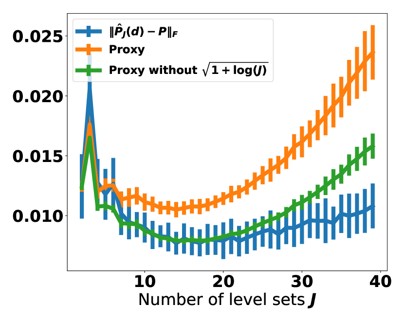
(b) $g(x)=0\vee(x_{1}-\frac{1}{10})+\frac{x_{2}+1}{2}$

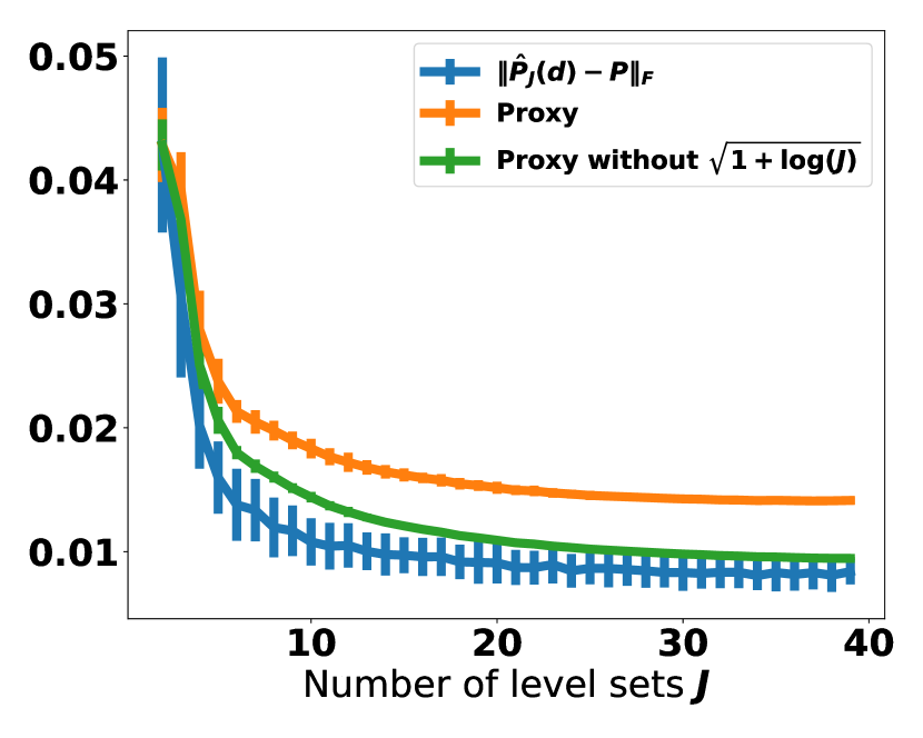
(c) $g(x)=x_{2}e^{\sin(x_{1})x_{2}+x_{2}}$

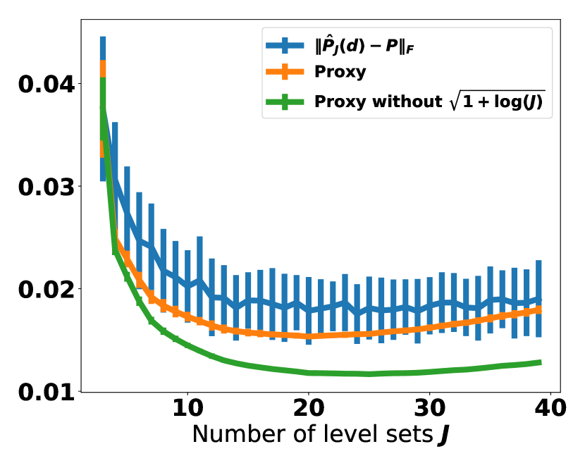
(d) $g(x)=x_{2}e^{\sin(x_{1})x_{2}+x_{3}}$

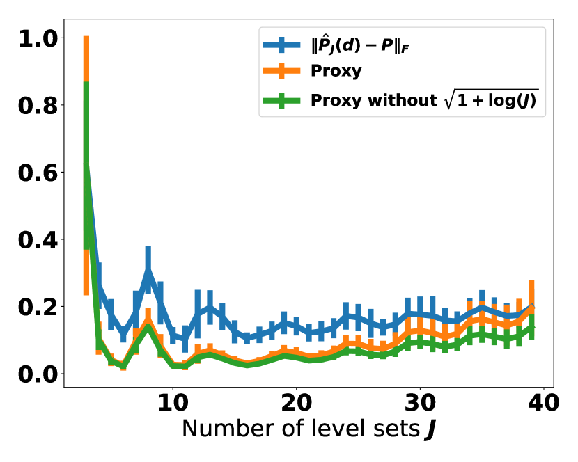
(e) Function (24)

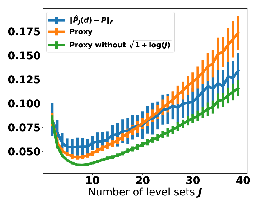
(f) $g(x)=\frac{\sin(x_{1})+\cos(x_{2}-\frac{1}{4})}{(1+x_{1}^{2})}$

Figure 2: Figures plot the function $J\mapsto\|\hat{P}_{{J}}(d)-P\|_{F}$ (blue), and compare it to the right hand side of (23) with (orange) and without (green) the union bound factor $\sqrt{1+\log(J)}$. The proxy is rescaled by a constant to match $\|\hat{P}_{{J}}(d)-P\|_{F}$ for $J=d$. Vertical bars indicate the standard deviation.

We now empirically study the tightness of (22) when considering a fixed number of samples $N$ but varying the number of level sets $J$. First, we develop a data-driven proxy to estimate the leading factor in (22) from a given data set. Afterwards, we compare the proxy with the true error on several synthetic examples.

Data-driven proxy

We have to replace $\gamma_{J}$, $\rho_{J,\ell}$, $\eta_{J,\ell}$, $\eta_{J,\ell}^{\perp}$ and $\kappa_{J,\ell}$ in (22) by quantities that can be estimated from data. The first three quantities are approximated by $\gamma_{J}\approx\lambda_{d}(\hat{M}_{J})$, $\rho_{J,\ell}\approx\hat{\rho}_{J,\ell}$ and $\eta_{J,\ell}\approx\|\hat{b}_{J,\ell}\|$, where the last replacement is motivated by the fact that $\eta_{J,\ell}$ is used to bound $\|\hat{b}_{J,\ell}\|\leq\|b_{J,\ell}\|+\|b_{J,\ell}-\hat{b}_{J,\ell}\|\lesssim\eta_{J,\ell}$ in the proofs of Theorems 6 and 7. Furthermore, we use the conditional sample covariance $\hat{\Sigma}_{J,\ell}$, and projections $\hat{P}_{J,\ell}:=\|{\hat{b}_{J,\ell}}\|^{-2}\hat{b}_{J,\ell}\hat{b}_{J,\ell}^{\top}$ and $\hat{Q}_{J,\ell}:=\mathsf{Id}-\hat{P}_{J,\ell}$, to compute an approximation to $\kappa_{J,\ell}$ by

$$\hat{\kappa}_{J,\ell}:=\max\left\{\left\|{\hat{P}_{J,\ell}\hat{\Sigma}_{J,\ell}\hat{P}_{J,\ell}}\right\|\left\|{\hat{P}_{J,\ell}\hat{\Sigma}_{J,\ell}^{\dagger}\hat{P}_{J,\ell}}\right\|,\left\|{\hat{Q}_{J,\ell}\hat{\Sigma}_{J,\ell}\hat{Q}_{J,\ell}}\right\|\left\|{\hat{Q}_{J,\ell}\hat{\Sigma}_{J,\ell}^{\dagger}\hat{Q}_{J,\ell}}\right\|\right\}.$$

Note that replacing squared sub-Gaussian norms with spectral norms of the corresponding covariance matrices can underestimate the true value of $\kappa_{J,\ell}$. The same strategy is used for $\eta_{J,\ell}^{\perp}$, i.e. we approximate $\eta_{J,\ell}^{\perp}$ by

$$\hat{\eta}_{J,\ell}^{\perp}:=\sqrt{\hat{\mathbb{E}}_{{\cal Y}_{J,\ell}}{\left(Y-\hat{\mathbb{E}}_{{\cal Y}_{J,\ell}}{Y}\right)^{2}}\left\|{\hat{Q}_{J,\ell}\hat{\Sigma}_{J,\ell}^{\dagger}\hat{Q}_{J,\ell}}\right\|}.$$

Combining everything, the data-driven proxy for the leading factor in (22) without the union bound factor $\sqrt{1+\log(J)}$ is given by

$$\frac{\sum_{\ell=1}^{J}\sqrt{\rho_{J,\ell}\kappa_{J,\ell}}\eta_{J,\ell}\eta_{J,\ell}^{\perp}}{\gamma_{J}}\approx\frac{\sum_{\ell=1}^{J}\sqrt{\hat{\rho}_{J,\ell}\hat{\kappa}_{J,\ell}}\left\|{\hat{b}_{J,\ell}}\right\|\hat{\eta}_{J,\ell}^{\perp}}{\lambda_{d}(\hat{M}_{J})}.$$ (23)

In order to reduce the variance in estimating (23), we further restrict the sum to level sets with at least $\left|{{\cal X}_{J,\ell}}\right|>5D$ samples in the experiments below.

Experiments

We sample $N=80000$ points from $\operatorname{Uni}({\{X:\left\|{X}\right\|\leq 1\}})$ in $D=20$ dimensions and set $Y=g(A^{\top}X)+\zeta$, where $\zeta\sim{\cal N}(0,10^{-4}\textrm{Var}(f(X)))$ and $A=[e_{1}|\ldots|e_{d}]$ with $e_{i}$ being the $i$-th standard basis vector. Each experiment is repeated 50 times and we report averaged results plus standard deviations for different link functions in Figures 2(a)-2(f).

We observe that the map $J\mapsto\|\hat{P}_{{J}}(d)-P\|_{F}$ initially decreases when increasing the number of level sets $J$ beyond $d$, and then either stalls, such as in Figures 2(a), 2(c), 2(e) and 2(d), or increases as in Figures 2(b) and 2(f). This behavior is captured well by the data driven proxy (23). Furthermore, even if the relation $J\mapsto\|\hat{P}_{{J}}(d)-P\|_{F}$ shows kinks as in Figure 2(e), where the link function is given by $g(x_{1},x_{2},x_{3})=\sum_{i=1}^{3}g_{i}(x_{i})$ with

$$g_{1}(x_{1}) =1(x_{1}<0)0.1x_{1}+1(x_{1}\geq 0)2.0\left(x_{1}-0.5\right)+0.05,$$ (24)

$$g_{2}(x_{2}) =1(x_{2}<0)2.0x_{2}+1(x_{2}\geq 0)0.1\left(x_{2}-0.5\right),$$

$$g_{3}(x_{3}) =1(x_{3}<0)5.0x_{3}+1(x_{3}\geq 0)0.1\left(x_{3}-0.2\right)+1,$$

the derived data-driven proxy reproduces the same behavior. The experiments suggest that Corollary 8 characterizes the influence of $J$ and the induced level set partition on the projection error well. Furthermore, they raise the question whether $J$, which minimizes the data-driven proxy (23), can be used for hyperparameter tuning in practice. This is an interesting direction for future work, because choosing $J$ for the related class of inverse regression based methods has been identified as a notoriously difficult problem, for which no good strategies exist [42].

4 Regression in the reduced space

In this section we return to the multi-index model $Y=g(A^{\top}X)+\zeta$ with $\mathbb{E}[\zeta|X]=0$ almost surely. Assumption $\zeta\mathchoice{\mathrel{\hbox to0.0pt{$\displaystyle\perp$\hss}\mkern 2.0mu{\displaystyle\perp}}}{\mathrel{\hbox to0.0pt{$\textstyle\perp$\hss}\mkern 2.0mu{\textstyle\perp}}}{\mathrel{\hbox to0.0pt{$\scriptstyle\perp$\hss}\mkern 2.0mu{\scriptstyle\perp}}}{\mathrel{\hbox to0.0pt{$\scriptscriptstyle\perp$\hss}\mkern 2.0mu{\scriptscriptstyle\perp}}}X|A^{\top}X$ is not strictly required in this part. The second step to estimate the model is to learn the link function $g$, while leveraging the approximated projection $\hat{P}\approx P$, e.g. constructed by using RCLS. We restrict our analysis to two popular and commonly used regressors, namely kNN-regression and piecewise polynomial regression. Our analysis reveals how the error $\|{\hat{P}-P}\|$ affects kNN and piecewise polynomials, if they are trained on perturbed data $\{(\hat{P}X_{i},Y_{i}):i\in[N]\}$ instead of $\{(PX_{i},Y_{i}):i\in[N]\}$. For simplicity, we assume $\hat{P}$ is deterministic and thus statistically independent of $\{(X_{i},Y_{i}):i\in[N]\}$. In practice, statistical independency can be ensured by using separate data sets for learning $\hat{P}$ and performing the subsequent regression task.

To study regression rates, smoothness properties of the link function play an important role. We use to the following standard definition [16].

Definition 9.

Let $f:\mathbb{R}^{D}\rightarrow\mathbb{R}$, $s_{1}\in\mathbb{N}_{0}$, $s_{2}\in(0,1]$ and $s=s_{1}+s_{2}$. We say $f$ is $(L,s)$-smooth if partial derivatives $\partial^{\alpha}f$ exist for all $\alpha\in\mathbb{N}_{0}^{D}$ with $\sum_{i}\alpha_{i}\leq s_{1}$, and for all $s$ with $\sum_{i}\alpha_{i}=s_{1}$ we have

$$\left|{\partial^{\alpha}f(z)-\partial^{\alpha}(z^{\prime})}\right|\leq L\left\|{z-z^{\prime}}\right\|^{s_{2}}.$$

The minimax rate for nonparametric estimation in $\mathbb{R}^{d}$ is well known [16, 49] and reads, for $(L,s)$-smooth regression function $f$,

$$\textrm{MSE}\left({\hat{f}},{f}\right):=\mathbb{E}\left(\hat{f}(X)-f(X)\right)^{2}\asymp N^{-\frac{2s}{2s+d}}.$$ (25)

Similarly, the rate is a lower bound for nonparametric estimation of the multi-index model with $\dim(P)=d$, because we are still left with a nonparametric regression problem in $\mathbb{R}^{d}$ once $P$ is identified. In the following, we provide conditions on $\|{\hat{P}-P}\|$ so that the optimal rate (25) is achieved, when training on perturbed data. In the analysis, we assume that $X$ is sub-Gaussian, $\left|{f(X)}\right|\leq 1$ almost surely, and $\textrm{Var}(\zeta|X)\leq\sigma_{\zeta}^{2}$ almost surely.

4.1 kNN-regression

Let $x$ be a new data point and denote a reordering of the indices by $1(x),\ldots,N(x)$ so that

$$\left\|{\hat{P}\left(x-X_{i(x)}\right)}\right\|\leq\left\|{\hat{P}\left(x-X_{j(x)}\right)}\right\|\textrm{ for all }j\geq i\textrm{ and all }i,$$

i.e. $i(x)$ is the $i$-th nearest neighbor to $x$ after projecting onto $\operatorname{Im}(\hat{P})$. The kNN-estimator is defined by $\hat{f}_{k}(x):=k^{-1}\sum_{i=1}^{k}Y_{i(x)}$ and the following theorem characterizes the influence of the projection error on the generalization performance. The proof resembles [16, 27] and is given in Appendix .5.

Theorem 10.

Let $g$ be $(L,s)$-smooth for $s\in(0,1]$, and $d>2s$. For $k=C_{k}N^{2s/(2s+d)}$, we obtain

$$\textrm{MSE}\left({\hat{f}_{k}},{f}\right)\leq C_{1}N^{-\frac{2s}{2s+d}}+C_{2}\log(N)\left\|{\hat{P}-P}\right\|^{2s},$$ (26)

where $C_{1}$ depends on $d,\sigma_{\zeta},\left\|{X}\right\|_{\psi_{2}},C_{k},L,s$, and $C_{2}$ additionally linearly on $D\left\|{X}\right\|_{\psi_{2}}^{2}$.

Remark 11 ($d>2s$ assumption).

The condition $d>2s$ in Theorem 10 is not due to the error $\|\hat{P}-P\|$, but arises from [27, Lemma 1], where ordinary kNN is analyzed for unbounded marginal distributions. It has been shown in [16] that achieving similar rates for $d\leq 2s$ requires an extra assumption of the marginal distribution of $X$ (boundedness does not suffice).

Remark 12 (Rate optimality).

Assuming $\|\hat{P}-P\|\in{\cal O}(N^{-1/2})$, we observe that the second term in (26) has order $N^{-s}$. Therefore, Theorem 10 ensures, up to the logarithmic factor, the optimal rate $N^{-2s/(2s+d)}$ for $d\geq 2$. The logarithmic factor disappears, if the marginal distribution of $X$ is bounded.

4.2 Piecewise polynomial regression

Piecewise polynomial estimators can be defined in different ways as they depend on a partition of the underlying space. Therefore we first have to describe the type of piecewise polynomials that we consider in the following.

Let $\hat{A}\in\mathbb{R}^{D\times d}$ contain column-wise an arbitrary orthonormal basis of $\operatorname{Im}(\hat{P})$. Denote by $\Delta_{l}$ the set of dyadic cubes in $\mathbb{R}^{d}$, i.e. the set of cubes with side length $2^{-l}$ and corners in the set $\{2^{-l}(v_{1},\ldots,v_{d}):v_{j}\in\mathbb{Z}\}$, and let $\Delta_{l}(R)\subseteq\Delta_{l}$ be the subset that has non-empty intersection with $\{\hat{A}^{\top}z:z\in B_{R}\}$, where $B_{R}=\{X\in\mathbb{R}^{D}:\left\|{X}\right\|\leq R\}$. Moreover, let ${\cal P}_{k}$ be the space of polynomials of degree $k$ in $\mathbb{R}^{d}$ and $1_{A}$ be the characteristic function of a set $A$. The function space of piecewise polynomials we consider is defined by

$${\cal F}(\hat{A},l,k,R)\!:=\!\left\{f\!:\!f(x)\!=\!1_{B_{R}}(x)\!\!\!\!\sum\limits_{c\in\Delta_{l}(R)}\!\!\!1_{c}\!\left(\hat{A}^{\top}x\right)\!p_{c}\left(\hat{A}^{\top}x\right),p_{c}\in{\cal P}_{k}\right\}\!.$$ (27)

To construct the estimator, we perform empirical risk minimization

$$\tilde{f}:=\operatorname*{argmin}_{h\in{\cal F}(\hat{A},l,k,R)}\sum\limits_{i=1}^{N}\left(h(X_{i})-Y_{i}\right)^{2},$$ (28)

and then set $\hat{f}(x):=T_{[-1,1]}(\tilde{f}(x))$, where $T_{[-1,1]}(u):=\textrm{sign}(u)(\left|{u}\right|\wedge 1)$. Note that piecewise polynomial estimators are typically analyzed after thresholding to avoid technical difficulties with potentially unbounded predictions (see also [6, 16]).

The following theorem characterizes the influence of $\|\hat{P}-P\|$ on the generalization performance of the estimator.

Theorem 13.

Let $g$ be $(L,s)$-smooth with $s=s_{1}+s_{2}$, $s_{1}\in\mathbb{N}_{0}$, $s_{2}\in(0,1]$. Choosing $l=\left\lceil\log_{2}(N)/(2s+d)\right\rceil$, $R^{2}=D\left\|{X}\right\|_{\psi_{2}}^{2}\log(N)$, and $k=s_{1}$ we get

$$\textrm{MSE}\left({\hat{f}},{f}\right) \!\leq\!C_{1}\log^{1\vee\frac{d}{2}}(N)N^{-\frac{2s}{2s+d}}+C_{2}\log(N)^{1\wedge s}\left\|{\hat{P}-P}\right\|^{2\wedge 2s}\!\!,$$ (29)

where the constants grow with $\sigma_{\zeta},d,s$, $L^{*}:=Ld^{s_{1}/2}(1-\|\hat{P}-P\|^{2})^{-s/2}$, and $C_{1}$ depends linearly on $(D\left\|{X}\right\|_{\psi_{2}}^{2})^{d/2}$, and $C_{2}$ linearly on $(D\left\|{X}\right\|_{\psi_{2}}^{2})^{1\wedge s}$.

Remark 14 (Boundedness and $\log$-factors).

For bounded $X$, the choice $R^{2}\asymp\log(N)$ is not required and $\log^{1\vee\frac{d}{2}}(N)$ reduces to $\log(N)$. Moreover, $D\left\|{X}\right\|_{\psi_{2}}^{2}$ can be replaced by the squared radius of a ball containing the support of $X$, which removes the dependency on $D$ entirely.

Remark 15 (Rate optimality).

Assuming $\|\hat{P}-P\|\in{\cal O}(N^{-1/2})$, we observe that the last term in (29) has order $N^{-s\wedge 1}$. Therefore, Theorem 13 ensures, up to $\log$-factors, the optimal rate $N^{-2s/(2s+d)}$ for $d=1$ and $s\geq\frac{1}{2}$, or $d\geq 2$ and $s>0$.

Proof sketch

The first step is to apply the following well-known result.

Theorem 16 (Theorem 11.3 in [16]).

Let ${\cal F}$ be a vector space of functions $f:\mathbb{R}^{D}\rightarrow[-1,1]$. Assume $Y=f(X)+\zeta$, $\mathbb{E}[Y|X]=f(X)$ and $\textrm{Var}(\zeta|X=x)\leq\sigma_{\zeta}^{2}$. Denote by $\tilde{f}$ the empirical risk minimizer in ${\cal F}$ over $N$ iid. copies of $(X,Y)$, and let $\hat{f}=T_{[-1,1]}(\tilde{f})$. Then there exists a universal constant $C$ such that

$$\textrm{MSE}\left({\hat{f}},{f}\right)\leq C(\sigma_{\zeta}^{2}\vee 1)\frac{\log(N)+\dim({\cal F})}{N}+C\inf\limits_{h\in{\cal F}}\textrm{MSE}\left({h},{f}\right).$$ (30)

The first term in (30) is the estimation error, which measures the deviation of the performance of the empirical risk minimizer to the best performing estimator in ${\cal F}$ when having access to the entire distribution. It decreases as more samples become available, but increases with the complexity of ${\cal F}$, here measured in terms of the dimensionality. It can be checked that ${\cal F}(\hat{A},l,k,R)$ is closed under addition and scalar multiplication and is thus a vector space. A basis can be constructed by combining the standard polynomial basis for each cell of the partition. Therefore $\dim({\cal F}(\hat{A},l,k,R))=\left|{\Delta_{l}(R)}\right|{{d+k}\choose k}$, where $\left|{\Delta_{l}(R)}\right|$ is the number of cells required to cover $\{\hat{A}^{\top}z:z\in B_{R}\}$. Lemma 24 in the Appendix proves $\left|{\Delta_{l}(R)}\right|\leq\lceil(2^{l+1}R)^{d}\rceil$ and therefore

$$\dim({\cal F}(\hat{A},l,k,R))\leq{{d+k}\choose k}\lceil(2^{l+1}R)^{d}\rceil.$$ (31)

The second term in (30) is the approximation error, which measures how well $f$ can be approximated by any function $h\in{\cal F}(\hat{A},l,k,R)$. Neglecting for a moment the perturbation $\hat{P}-P$, it is known that a piecewise Taylor expansion of $g$ can be used to approximate $g$ with an accuracy that increases as the underlying partition is refined. The main difficulty in our case is to define a piecewise polynomial function $h\in{\cal F}(\hat{A},l,k,R)$ that approximates $g(A^{\top}x)$, despite the fact that $h$ depends on coordinates $\hat{A}^{\top}x$ instead of $A^{\top}x$.

To define such a function, we first prove the existence of a function $g^{*}$ that approximates $g$ uniformly well, when being evaluated on $\hat{A}^{\top}x$. Precisely, Lemma 25 in the Appendix shows

$$\left|{g^{*}(\hat{A}^{\top}x)-g(A^{\top}x)}\right|\leq L^{*}\left\|{x}\right\|^{1\wedge s}\|\hat{P}-P\|^{1\wedge s},$$

for some $(L^{*},s)$-smooth function $g^{*}$. Now, by approximating $g^{*}$ through a piecewise Taylor expansion, we can construct a function $h\in{\cal F}(\hat{A},l,k,R)$ which, using choices $l,\,k$ and $R$ as in Theorem 13, satisfies

$$\textrm{MSE}\left({h},{f}\right)\leq C_{1}N^{-\frac{2s}{2s+d}}+C_{2}\log^{1\wedge s}(N)\left\|{\hat{P}-P}\right\|^{2\wedge 2s},$$ (32)

for constants $C_{1}$ depending on $L^{*},d,s$, and $C_{2}$ depending on $L^{*}$ and linearly on $(D\left\|{X}\right\|_{\psi_{2}}^{2})^{1\wedge s}$ (see Corollary 27). The proof of Theorem 13 concludes by combining Theorem 16, the dimensionality bound (31), and the approximation error bound (32) (see Appendix .6).

5 Numerical experiments

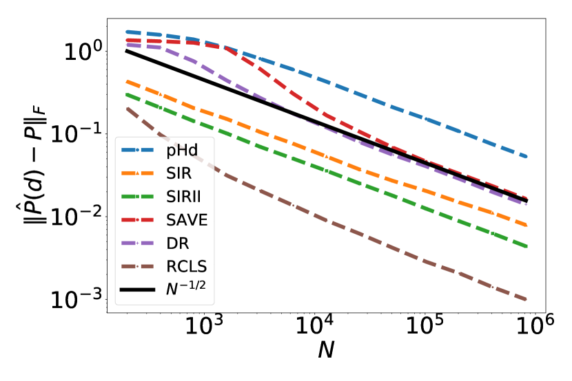
(a) $g(x)=\frac{x_{2}}{1+(x_{1}-1)^{2}}$

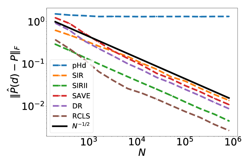
(b) $g(x)=0\vee(x_{1}-\frac{1}{10})+\frac{x_{2}+1}{2}$

(c) $g(x)=x_{2}e^{\sin(x_{1})x_{2}+x_{2}}$

(d) $g(x)=x_{2}e^{\sin(x_{1})x_{2}+x_{3}}$

(e) Function (24)

(f) $g(x)=\frac{\sin(x_{1})+\cos(x_{2}-1/4)}{(1+x_{1}^{2})}$

Figure 3: Projection errors $\|\hat{P}_{{J}}(d)-P\|_{F}$ for different methods as a function of the sample size $N$. Except PHD, most estimators achieve an expected $N^{-1/2}$ convergence rate on all problems. RCLS and SIRII stand out by consistently achieving first and second best performances.

We now compare RCLS to the most prominent inverse regression based techniques SIR, SIRII, SAVE, pHd and DR that have been described extensively in Section 1.1. In the first part we consider synthetic problems and we directly assess the performance by evaluating $\|\hat{P}_{{J}}(d)-P\|_{F}$, since the true index space is known. In the second part, we consider real data sets from the UCI data set repository. Here, the true index space is unknown, and we instead compare recovered spaces $\operatorname{Im}(\hat{P})$ by measuring the predictive performance of kNN-regression, when trained on $\{(\hat{P}X_{i},Y_{i}):i\in[N]\}$. In both cases we construct the partition ${\cal R}_{J,\ell}$ using dyadic cells in the response domain as described in Section 2. The source code for all experiments is readily available at https://github.com/soply/sdr_toolbox and https://github.com/soply/mim_experiments.

5.1 Synthetic data sets

We sample $X\sim\textrm{Uni}(\{X:\left\|{X}\right\|\leq 1\})$ in $\mathbb{R}^{20}$, and generate the response by $Y=g(A^{\top}X)+\zeta$ for several functions $g$ and $\zeta\sim{\cal N}(0,0.01^{2}{\operatorname{Var}}(g(A^{\top}X)))$. The index space is $A=[e_{1}|\ldots|e_{d}]\in\mathbb{R}^{D\times d}$ where $e_{i}$ is the $i$-th standard basis vector. The hyperparameter $J$ is chosen optimally for SIR, SIRII, SAVE, DR and RCLS to minimize the projection error within $J\in[100]$. No parameter is required for pHd.

We report projection errors averaged over 100 repetitions of the same experiment in Figures 3(a) - 3(f). First, notice that most estimators (except pHd in some cases) achieve an expected $N^{-1/2}$ rate on all problems. pHd fails to detect linear trends and therefore fails to detect the index space in some cases. RCLS achieves the best performance in Figures 3(a)-3(c), is tied with SIRII in Figure 3(d), and runner up to SIRII in the remaining cases.

In Figures 3(a)-3(c), where RCLS improves upon competitors, we observe (temporary) convergence speeds beyond $N^{-1/2}$. This can be explained by recent results in [25], when recognizing that the multi-index models in 3(a)-3(c) have approximately monotone single-index structure if we restrict $(X,Y)$ to small level sets $Y\in{\cal R}_{J,\ell}$. More precisely, [25] shows that the convergence rate of RCLS can be temporarily as large as $\log(N)N^{-1}$, if the data follows a monotone single-index model. The reason for this increased convergence speed is that the variance of the local least squares estimator decreases quadratically in the length of the level set ${\cal R}_{J,\ell}$ [25, 26], and hence the convergence speed may exceed $N^{-1/2}$ when choosing $J$ as an increasing function of $N$. These observations suggest that RCLS is particularly suited for multi-index models where we assume a response-local single-index structure to be a good fit.

5.2 Real data sets

Characteristics	Airquality	Ames		Boston	Concrete		Skillcraft	Yacht
$\log$-TF	No	Yes		Yes	No		Yes	Yes
$D,\ N$	$11,\ 7393$	$7,\ 1197$		$12,\ 506$	$8,\ 1030$		$16,\ 3338$	$6,\ 307$
Factor	$10^{-1}$	$10^{5}$		$10^{1}$	$10^{1}$		$10^{2}$	$10^{1}$
$\bar{Y}\pm\textrm{STD}(Y)$	$9.95\pm 4.03$	$1.74\pm 0.67$		$1.27\pm 0.71$	$3.58\pm 1.67$		$1.15\pm 0.48$	$1.05\pm 1.51$
Baselines
LinReg	$1.22\pm 0.03$	$\bf{0.23\pm 0.02}$		$0.50\pm 0.11$	$1.06\pm 0.06$		$0.14\pm 0.03$	$0.22\pm 0.07$
kNN	$1.03\pm 0.02$	$0.26\pm 0.03$		$0.41\pm 0.06$	$0.89\pm 0.08$		$0.17\pm 0.01$	$0.76\pm 0.11$
$k$	$25.0$	$9.8$		$6.8$	$5.5$		$9.8$	$1.1$
SDR + KNN
pHd	$1.01\pm 0.04$	$0.29\pm 0.04$		$0.43\pm 0.06$	$0.89\pm 0.04$		$0.26\pm 0.01$	$0.70\pm 0.18$
$d$	$10.2$	$6.5$		$7.55$	$6.65$		$7.0$	$5.4$
$k$	$10.0$	$7.7$		$5.3$	$4.0$		$16.4$	$1.7$
SIR	$0.59\pm 0.02$	$0.24\pm 0.04$		$0.42\pm 0.07$	$0.87\pm 0.06$		$0.08\pm 0.01$	$0.18\pm 0.07$
$d$	$6.15$	$1.4$		$4.8$	$6.1$		$1.85$	$1.15$
$k$	$10.0$	$11.4$		$6.95$	$3.7$		$11.4$	$8.4$
$J$	$10.3$	$10.8$		$8.6$	$9.8$		$7.65$	$8.6$
SIRII	$0.87\pm 0.02$	$0.27\pm 0.04$		$0.44\pm 0.07$	$0.89\pm 0.06$		$0.29\pm 0.03$	$0.53\pm 0.21$
$d$	$11.0$	$7.0$		$6.65$	$8.0$		$2.75$	$2.8$
$k$	$10.0$	$8.45$		$5.3$	$4.0$		$16.75$	$6.7$
$J$	$12.0$	$9.8$		$8.2$	$10.4$		$3.75$	$4.6$
SAVE	$0.58\pm 0.01$	$0.25\pm 0.04$		$0.44\pm 0.05$	$0.79\pm 0.09$		$0.09\pm 0.01$	$0.18\pm 0.04$
$d$	$6.0$	$2.9$		$7.55$	$3.85$		$4.65$	$1.7$
$k$	$10.0$	$10.7$		$6.35$	$3.2$		$9.5$	$7.35$
$J$	$13.4$	$12.0$		$9.9$	$8.3$		$8.75$	$8.7$
DR	$0.58\pm 0.02$	$0.24\pm 0.03$		$\bf{0.40\pm 0.07}$	$0.75\pm 0.08$		$0.08\pm 0.01$	$0.18\pm 0.06$
$d$	$5.85$	$2.15$		$5.45$	$3.35$		$2.6$	$1.75$
$k$	$10.0$	$11.3$		$6.8$	$3.7$		$14.9$	$6.55$
$J$	$12.6$	$12.0$		$10.2$	$8.5$		$9.3$	$8.75$
RCLS	$\bf{0.51\pm 0.03}$	$0.25\pm 0.03$		$0.41\pm 0.06$	$\bf{0.72\pm 0.06}$		$\bf{0.07\pm 0.01}$	$\bf{0.17\pm 0.06}$
$d$	$5.4$	$1.9$		$5.1$	$3.25$		$2.95$	$1.75$
$k$	$10.0$	$13.55$		$11.0$	$4.3$		$9.15$	$5.6$
$J$	$11.9$	$6.4$		$5.7$	$5.7$		$3.2$	$7.3$

Table 2: RMSE, standard deviation, and cross-validated hyperparameters, over $20$ repetitions for several estimators and UCI repository data sets. Values for $d$, $k$, $J$ are averages over different runs of each experiment. First $5$ rows describe the data sets and their characteristics, and the remaining rows contain the results. For a simplified presentation, we divide the mean and STD of RMSE, and the mean and STD of the data (5th row) by the value in row Factor.

To compare RCLS with inverse regression based competitors on real data sets, we first compute an index space and then compare the predictive performance when training a kNN-regressor on projected samples. More precisely, we conduct the following steps.

1. Split the data set $\{(X_{i},Y_{i}):i\in[N]\}$ into training and test set ${\cal X}_{\textrm{Train}},{\cal Y}_{\textrm{Train}}$, and ${\cal X}_{\textrm{Test}},{\cal Y}_{\textrm{Test}}$

2. Use pHd, SIR, SIRII, SAVE, DR, RCLS on the training set to compute an index space $\hat{A}$

3. Train a kNN-regressor using $\{(\hat{A}^{\top}X_{i},Y_{i}):X_{i}\in{\cal X}_{\textrm{Train}}\}$

4. Crossvalidate over hyperparameters $d$ (index space dimension), $k$ (kNN parameter), and $J$ (number of level sets) using a hold-out validation set of the training data

5. Compute the root mean squared error (RMSE) of the kNN-regressor on the test set

The test set contains $15\%$ of the data, while cross-validation is performed using a $10$-fold splitting strategy. Each experiment is repeated 20 times and we report the mean and standard deviation.

We consider the UCI data sets Airquality, Ames-housing, Boston-housing, Concrete, Skillcraft and Yacht. We standardize the components of $X$ to $[-1,1]$ and potentially perform a $\log$ transformation of $Y$ if the marginal has sparsely populated tails. This is indicated by the $\log$-TF row in Table 2. For some data sets, we also exclude features with missing values, or, in the case of Ames, we exclude some irrelevant and categorical features to reduce the complexity of the data set. Preprocessed data sets can be found at https://github.com/soply/db_hand.

The RMSE and cross-validated hyperparameters are presented in Table 2. To have robust baselines for comparison, we also compute the RMSE of standard linear regression and kNN regression. We first see that applying a dimension reduction technique improves the performance of linear regression and ordinary kNN significantly on data sets Airquality, Concrete, Skillcraft and Yacht. Furthermore, on these data sets, RCLS convinces by achieving the best results among all competitors. Runner-up is DR, where SIR and SAVE share third and fourth place. The results of pHd and SIRII are not convincing on most data sets.

The study confirms that RCLS is a viable alternative to prominent inverse regression methods. The data sets were chosen because one-dimensional maps $e_{i}^{\top}X\mapsto Y$, where $e_{i}$ is the $i$-th standard basis vector, show a certain degree of monotonicity. We believe that this promotes a response-local monotone single-index structure, which is beneficial for the accuracy of the RCLS approach as briefly discussed in Section 5.1.

.3 Probabilistic results

This section contains some probabilistic auxiliary results used in the paper.

Lemma 17.

If $Z\in\mathbb{R}^{D}$ is sub-Gaussian and $E$ an event with $\mathbb{P}(E)>0$, then $Z|E$ is sub-Gaussian with $\left\|{Z|E}\right\|_{\psi_{2}}\leq\left\|{Z}\right\|_{\psi_{2}}\mathbb{P}(E)^{-1}$.

Proof.

Assume without loss of generality $Z\in\mathbb{R}$. The result for the vector then follows by the definition. We use the characterization of sub-Gaussianity by the moment bound in [50, Proposition 2.5.2, b)]. So let $p\geq 1$. By the law of total expectation it follows that $\mathbb{E}[\left|{Z}\right|^{p}]=\mathbb{E}[\left|{Z}\right|^{p}|E]\mathbb{P}(E)+\mathbb{E}[\left|{Z}\right|^{p}|E^{C}]\mathbb{P}(E^{C})\geq\mathbb{E}[\left|{Z}\right|^{p}|E]\mathbb{P}(E)$. Dividing $\mathbb{P}(E)$ and using monotonicity of the $p$-th root

$$\left(\mathbb{E}[\left|{Z}\right|^{p}|E]\right)^{1/p}\leq\frac{\left(\mathbb{E}[\left|{Z}\right|^{p}]\right)^{1/p}}{\mathbb{P}(E)^{1/p}}\leq\frac{\left(\mathbb{E}[\left|{Z}\right|^{p}]\right)^{1/p}}{\mathbb{P}(E)}\leq C\frac{\left\|{Z}\right\|_{\psi_{2}}\sqrt{p}}{\mathbb{P}(E)},$$

where $C$ is some universal constant, the second inequality follows from $\mathbb{P}(E)\leq 1$, and the third from the sub-Gaussianity of $Z$. ∎

Lemma 18.

If $X\in\mathbb{R}^{D}$ is sub-Gaussian, so is $\left\|{X}\right\|$, with $\|\|X\|\|_{\psi_{2}}\leq\sqrt{D}\|X\|_{\psi_{2}}$.

Proof.

Using Hölder’s inequality and the sub-Gaussianity of $X$ we compute

$$\mathbb{E}\left[\exp\left(\frac{\|X\|^{2}}{D\|X\|_{\psi_{2}}^{2}}\right)\right]=\mathbb{E}\left[\prod_{i=1}^{D}\exp\left(\frac{|e_{i}^{T}X|^{2}}{D\|X\|_{\psi_{2}}^{2}}\right)\right]\leq\left(\prod_{i=1}^{D}\mathbb{E}\left[\exp\left(\frac{|e_{i}^{T}X|^{2}}{\|X\|_{\psi_{2}}^{2}}\right)\right]\right)^{1/D}\leq 2.\qed$$

Lemma 19.

Fix $u>0$, $\varepsilon>0$. Let $Y\in\mathbb{R}$ be a random variable, ${\cal R}$ an interval, and $\hat{\mathbb{P}}(Y\in{\cal R}):=\left|{\{Y_{i}\in{\cal R}\}}\right|N^{-1}$ the empirical estimate of $\mathbb{P}(Y\in{\cal R})$ based on $N$ iid. samples. Then

$$\mathbb{P}\left(\left|{\hat{\mathbb{P}}(Y\in{\cal R})-\mathbb{P}(Y\in{\cal R})}\right|\leq\varepsilon\right)\geq 1-\exp(-u)\hskip 3.0pt\textrm{ if }N>Cu\varepsilon^{-2},$$ (33)

$$\mathbb{P}\left(\left|{\hat{\mathbb{P}}(Y\in{\cal R})-\mathbb{P}(Y\in{\cal R})}\right|\leq\frac{1}{2}\mathbb{P}(Y\in{\cal R})\right)\geq 1-2\exp(-u)\hskip 3.0pt\textrm{ if }N>C\frac{u}{\mathbb{P}(Y\in{\cal R})}.$$ (34)

Proof.

For (33), we write $\hat{\mathbb{P}}(Y\in{\cal R})-\mathbb{P}(Y\in{\cal R})$ as a sum of iid. centred random variables $Z_{i}:=1_{{\cal R}}(Y_{i})-\mathbb{P}(Y\in{\cal R})$ that are bounded by $\left|{Z_{i}}\right|\leq 1$. The result follows by applying Hoeffding’s inequality [50, Theorem 2.2.6]. For the Chernoff-type bound (34) we recognize $\hat{\mathbb{P}}(Y\in{\cal R})N$ as a sum of independent random variables $1\{Y_{i}\in{\cal R}\}$ with values in $\{0,1\}$, and $\mathbb{E}[\hat{\mathbb{P}}(Y\in{\cal R})N]=\mathbb{P}(Y\in{\cal R})N$. [44] provides the bound

$$\mathbb{P}\left(\left|{\hat{\mathbb{P}}(Y\in{\cal R})N-\mathbb{P}(Y\in{\cal R})N}\right|\geq\frac{1}{2}\mathbb{P}(Y\in{\cal R})N\right)\leq 2\exp\left(-\frac{\mathbb{P}(Y\in{\cal R})N}{12}\right),$$

and the result follows division by $N$, and $N>12\mathbb{P}(Y\in{\cal R})^{-1}u$. ∎

.4 Differences of projections

We gather two auxiliary results to rewrite the norm of differences of projections.

Lemma 20.

Let $A$ and $B$ be subspaces with $\dim(A)=\dim(B)$, and let $P_{A}$ and $P_{B}$ the corresponding orthogonal projections. For $P_{A^{\perp}}=\mathsf{Id}-P_{A}$ we get $\left\|{P_{A}-P_{B}}\right\|=\left\|{P_{A^{\perp}}P_{B}}\right\|.$

Proof.

Assume $\left\|{\left(\mathsf{Id}-P_{A}\right)P_{B}}\right\|=\left\|{P_{A^{\perp}}P_{B}}\right\|<1$ first. Then the first case of Theorem 6.34 in Chapter 1 in [24] applies. Note that the second case can be ruled out since $P_{A}$ can not map $\operatorname{Range}({P_{B}})$ one-to-one onto a proper subspace of $V\subset\operatorname{Range}({P_{A}})$ because $\dim(V)<\dim(\operatorname{Range}({P_{A}}))=\dim(\operatorname{Range}({P_{B}}))$ according to the assumption. Thus, in the first case it follows that

$$\left\|{\left(\mathsf{Id}-P_{A}\right)P_{B}}\right\|=\left\|{\left(\mathsf{Id}-P_{B}\right)P_{A}}\right\|=\left\|{P_{A}-P_{B}}\right\|.$$

Now let $\left\|{P_{A^{\perp}}P_{B}}\right\|=1$. Then there exists $v\in\mathbb{S}^{D}$ such that $\left\|{P_{A^{\perp}}P_{B}v}\right\|=\left\|{v}\right\|$. Since

$$\left\|{v}\right\|\geq\left\|{P_{B}v}\right\|\geq\left\|{P_{A^{\perp}}P_{B}v}\right\|=\left\|{v}\right\|,$$

it follows that $\left\|{P_{B}v}\right\|=\left\|{v}\right\|$, and thus $P_{B}v=v$ because $P_{B}$ is a projection. With the same argument we deduce also $P_{A^{\perp}}v=v$, and then

$$\left(P_{A}-P_{B}\right)v=P_{A}v-P_{B}v=0-v=v$$

implies $\left\|{P_{A}-P_{B}}\right\|=1=\left\|{P_{A^{\perp}}P_{B}}\right\|$. ∎

Lemma 21.

Let $A$ and $B$ be subspaces with $m=\dim(A)=\dim(B)$, and let $P_{A}$ and $P_{B}$ the corresponding orthogonal projections. For $P_{A^{\perp}}=\mathsf{Id}-P_{A}$ we get $\left\|{P_{A}-P_{B}}\right\|_{F}=\sqrt{2}\left\|{P_{A^{\perp}}P_{B}}\right\|_{F}$.

Proof.

With slight abuse of notation we denote $A,B\in\mathbb{R}^{D\times m}$ two orthonormal bases of $A$ respectively $B$ such that $P_{A}=AA^{\top}$, $P_{B}=BB^{\top}$. Now, denote $A^{\top}B=U(cos(\theta))V^{\top}$ where $\cos(\theta)\in\mathbb{R}^{m\times m}$ is the diagonal matrix containing the principal angles $\theta_{i}$ [17]. From [17] we obtain the identity $1/2\left\|{P_{A}-P_{B}}\right\|_{F}^{2}=m-\sum_{i=1}^{m}\cos^{2}(\theta_{i})$. Doing some further manipulations we get

$$\frac{1}{2}\left\|{P_{A}-P_{B}}\right\|_{F}^{2} =m-\sum_{i=1}^{m}\cos^{2}(\theta_{i})=m-\left\|{A^{\top}B}\right\|_{F}^{2}$$

$$=m-\textrm{Trace}(B^{\top}AA^{\top}B)=m-\textrm{Trace}(AA^{\top}BB^{\top})$$

$$=m-\textrm{Trace}(P_{A}P_{B})=m-\textrm{Trace}((\mathsf{Id}-P_{A^{\perp}})P_{B})$$

$$=m-\textrm{Trace}(P_{B})+\textrm{Trace}(P_{A^{\perp}}P_{B}).$$

The result follows by $\textrm{Trace}(P_{B})=\dim(B)=m$ and $\textrm{Trace}(P_{A^{\perp}}P_{B})=\left\|{P_{A^{\perp}}P_{B}}\right\|_{F}^{2}$. ∎

.5 Proof of Theorem 10

Proof of Theorem 10.

Denote $S_{X}=\{X_{i}:i\in[N]\}$ and $\tilde{f}_{k}(x)=\mathbb{E}[\hat{f}_{k}(x)|S_{X}]=\sum_{i=1}^{k}f(X_{i(x)})$ for fixed $x$. We first decompose (randomness is in the $\zeta_{i}$’s)

$$\mathbb{E}\left[\left(\hat{f}_{k}(x)-f(x)\right)^{2}\Big{|}S_{X}\right]=\mathbb{E}\left[\left(\hat{f}_{k}(x)-\tilde{f}_{k}(x)\right)^{2}\Big{|}S_{X}\right]+\left(\tilde{f}_{k}(x)-f(x)\right)^{2},$$

and then use the towering property of conditional expectations to obtain

$$\mathbb{E}\left(\hat{f}_{k}(X)-f(X)\right)^{2} =\mathbb{E}\mathbb{E}\left[\left(\hat{f}_{k}(X)-f(X)\right)^{2}\Big{|}{\cal S}_{X}\right]$$

$$=\mathbb{E}\mathbb{E}\left[\left(\hat{f}_{k}(X)-\tilde{f}_{k}(X)\right)^{2}\Big{|}{\cal S}_{X}\right]+\mathbb{E}\left(\tilde{f}_{k}(X)-f(X)\right)^{2}$$

$$=\mathbb{E}\left(\hat{f}_{k}(X)-\tilde{f}_{k}(X)\right)^{2}+\mathbb{E}\left(\tilde{f}_{k}(X)-f(X)\right)^{2}$$

Since $\mathbb{E}\zeta_{i}=0$, $\zeta_{i}\mathchoice{\mathrel{\hbox to0.0pt{$\displaystyle\perp$\hss}\mkern 2.0mu{\displaystyle\perp}}}{\mathrel{\hbox to0.0pt{$\textstyle\perp$\hss}\mkern 2.0mu{\textstyle\perp}}}{\mathrel{\hbox to0.0pt{$\scriptstyle\perp$\hss}\mkern 2.0mu{\scriptstyle\perp}}}{\mathrel{\hbox to0.0pt{$\scriptscriptstyle\perp$\hss}\mkern 2.0mu{\scriptscriptstyle\perp}}}\zeta_{j}$ and $\textrm{Var}(\zeta_{i}|X=x)\leq\sigma_{\zeta}^{2}$, the first term satisfies the bound

$$\mathbb{E}\left(\hat{f}_{k}(X)-\tilde{f}_{k}(X)\right)^{2}=\textrm{Var}\left(\frac{1}{k}\sum\limits_{i=1}^{k}\zeta_{i(X)}\right)\leq\frac{\sigma_{\zeta}^{2}}{k}=C_{k}^{-1}\sigma_{\zeta}^{2}N^{-\frac{2s}{2s+d}}.$$

For $\mathbb{E}\left(\tilde{f}_{k}(X)-f(X)\right)^{2}$, we recall that $f(X)=g(A^{\top}X)$ for some $(L,s)$-smooth $g$, which implies

$$\mathbb{E}\left(\tilde{f}_{k}(X)-f(X)\right)^{2} =\mathbb{E}\left(\frac{1}{k}\sum\limits_{i=1}^{k}g(A^{\top}X_{i(X)})-g(A^{\top}X)\right)^{2}$$

$$\leq 4L^{2}\mathbb{E}\left(\frac{1}{k}\sum\limits_{i=1}^{k}\min\left\{\left\|{A^{\top}\left(X_{i(X)}-X\right)}\right\|^{s},1\right\}\right)^{2},$$

where the $4$ can be injected since $\left|{f(X)}\right|\leq 1$ almost surely. To bound this term further we have to replace $\{X_{i(X)}:i\in[k]\}$ (the $k$ closest samples wrt to $\hat{d}(\cdot,X):=\|\hat{P}\left(\cdot-X\right)\|$) by the $k$ closest samples based on $d(\cdot,X):=\|P\left(\cdot-X\right)\|$. So let $\tilde{X}_{i(X)}$ denote the $i$-th closest sample to $X$ based on $d$, and let further $\delta:=\left\|{\hat{P}-P}\right\|$. Since

$$\left|{d(X,X^{\prime})-\hat{d}(X,X^{\prime})}\right|\leq\left\|{(P-\hat{P})(X-X^{\prime})}\right\|\leq\delta\left\|{X-X^{\prime}}\right\|,$$

and $(a+b)^{s}\leq a^{s}+b^{s}$ for $s\leq 1$, we can bound

$$\sum\limits_{i=1}^{k}\min\{d(X_{i(X)},X)^{s},1\} \leq\sum\limits_{i=1}^{k}\min\{\hat{d}(X_{i(X)},X)^{s}+\delta^{s}\max_{i\in[N]}\left\|{X_{i}-X}\right\|^{s},1\}$$

$$\leq\sum\limits_{i=1}^{k}\min\{\hat{d}(\tilde{X}_{i(X)},X)^{s}+\delta^{s}\max_{i\in[N]}\left\|{X_{i}-X}\right\|^{s},1\}$$

$$\leq\sum\limits_{i=1}^{k}\min\left\{d(\tilde{X}_{i(X)},X)^{s}+2\delta^{s}\max_{i\in[N]}\left\|{X_{i}-X}\right\|^{s},1\right\},$$

where in the second inequality we used that $X_{i(X)}$ minimizes the distance to $X$ measured in $\hat{d}$, and can therefore be replaced by $\tilde{X}_{i(X)}$. Denoting $\Delta_{X,N}:=2\delta^{s}\max_{i\in[N]}\left\|{X_{i}-X}\right\|^{s}$ and using $(\sum_{i=1}^{k}b_{i})^{2}\leq k\sum_{i=1}^{k}b_{i}^{2}$ for arbitrary $b_{i}$’s, we get

$$\mathbb{E}\left(\hat{f}_{k}(X)-f(X)\right)^{2} \leq 4L^{2}\mathbb{E}\left(\frac{1}{k}\sum\limits_{i=1}^{k}\min\{d(\tilde{X}_{i(X)},X)^{s}+\Delta_{X,N},1\}\right)^{2}$$ (35)

$$\leq\frac{4L^{2}}{k}\sum\limits_{i=1}^{k}\mathbb{E}\min\{(d(\tilde{X}_{i(X)},X)^{s}+\Delta_{X,N})^{2},1\}$$

$$\leq\frac{8L^{2}}{k}\sum\limits_{i=1}^{k}\mathbb{E}\min\{d(\tilde{X}_{i(X)},X)^{2s},1\}+\frac{8L^{2}}{k}\sum\limits_{i=1}^{k}\mathbb{E}\Delta_{X,N}^{2}.$$

For the first term, we proceed as in [16, 27] by randomly splitting the data set $\{X_{i}:i\in[N]\}$ into $k+1$ sets, where the first $k$ sets contain $\lfloor N/k\rfloor$ samples. Then we let $X^{*}_{i(X)}$ denote the nearest neighbor to $X$ (measured in $d$) within the $i$-th set. Since $\{\tilde{X}_{i(X)}:i\in[k]\}$ are by definition the closest $k$ samples (measured in $d$), we can bound

$$\frac{8L^{2}}{k}\sum\limits_{i=1}^{k}\mathbb{E}\min\{d(\tilde{X}_{i(X)},X)^{2s},1\} \leq\frac{8L^{2}}{k}\sum\limits_{i=1}^{k}\mathbb{E}\min\{d(X^{*}_{i(X)},X)^{2s},1\}$$

$$=8L^{2}\mathbb{E}\min\left\{\left\|{P\left(X^{*}_{1(X)}-X\right)}\right\|^{2s},1\right\},$$

where the last equality uses that the distribution of $X^{*}_{i(X)}-X$ is independent of the set index $i$. Since $\left\|{P(\cdot)}\right\|=\left\|{A^{\top}(\cdot)}\right\|$, $d>2s$ by assumption, and

$$\mathbb{E}\left\|{A^{\top}X}\right\|^{\beta}=\mathbb{E}\left\|{X}\right\|^{\beta}\lesssim\left\|{X}\right\|_{\psi_{2}}^{\beta}\beta^{\beta/2}$$

for any $\beta\geq 1$ by the sub-Gaussianity of $X$ (see [50, Proposition 2.5.2]), Lemma 1 in [27] implies the existence of a constant $C_{1}=C_{1}(d,s,\left\|{X}\right\|_{\psi_{2}})$ satisfying

$$\mathbb{E}\min\left\{\left\|{P\left(X^{*}_{1(X)}-X\right)}\right\|^{2s},1\right\} =\mathbb{E}\min\left\{\left\|{A^{\top}\left(X^{*}_{1(X)}-X\right)}\right\|^{2s},1\right\}$$

$$\leq C_{1}\left(\frac{k}{N}\right)^{\frac{2s}{d}}=C_{1}C_{k}^{\frac{2s}{d}}N^{-\frac{2s}{2s+d}}.$$

It remains to bound the last term in (35). Denote for short $\sigma_{X}=\left\|{X}\right\|_{\psi_{2}}$. We first compute that

$$\mathbb{E}\Delta_{X,N}^{2} =\int_{0}^{\infty}\mathbb{P}\left(\Delta_{X,N}^{2}>u\right)du=\int_{0}^{\infty}\mathbb{P}\left(\max_{i=1,\ldots,N}\left\|{X_{i}-X}\right\|^{2s}>\frac{u}{4\delta^{2s}}\right)du.$$

We can control this probability by using the sub-Gaussianity of $X$. More precisely, since $X$ is sub-Gaussian, $X_{i}-X$ is sub-Gaussian (norm changing only by a universal constant), and Lemma 18 implies that $\|\left\|{X_{i}-X}\right\|\|_{\psi_{2}}\leq C\sqrt{D}\sigma_{X}$. Taking the square, and using [50, Lemma 2.7.6], we obtain

$$\|\left\|{X_{i}-X}\right\|^{2}\|_{\psi_{1}}\leq\|\left\|{X_{i}-X}\right\|\|_{\psi_{2}}^{2}\leq CD\sigma_{X}^{2}.$$

To bound the integral, we first split $[0,\infty]$ into $[0,\nu D\sigma_{X}^{2}\log(N)\delta^{2s}]$ and $[\nu D\sigma_{X}^{2}\log(N)\delta^{2s},\infty]$ for some $\nu>4\max\{\frac{1}{D\sigma_{X}^{2}\log(N)},C\}$, which yields

$$\mathbb{E}\Delta_{X,N}^{2} \leq\int_{\nu D\sigma_{X}^{2}\log(N)\delta^{2s}}^{\infty}\mathbb{P}\left(\max_{i\in[N]}\left\|{X_{i}-X}\right\|^{2s}>\frac{u}{4\delta^{2s}}\right)du+\nu D\sigma_{X}^{2}\log(N)\delta^{2s}.$$

For the first term we realize that $u>\nu D\sigma_{X}^{2}\log(N)\delta^{2s}>4\delta^{2s}$ implies

$$\mathbb{P}\left(\max_{i=1,\ldots,N}\left\|{X_{i}-X}\right\|^{2s}>\frac{u}{4\delta^{2s}}\right)\leq\mathbb{P}\left(\max_{i=1,\ldots,N}\left\|{X_{i}-X}\right\|^{2}>\frac{u}{4\delta^{2s}}\right).$$

Then the sub-Exponentiality of $\|X-X_{i}\|^{2}$ and a union bound argument over $i\in[N]$ give

$$\mathbb{E}\Delta_{X,N}^{2} \leq\int_{\nu D\sigma_{X}^{2}\log(N)\delta^{2s}}^{\infty}\mathbb{P}\left(\max_{i\in[N]}\left\|{X_{i}-X}\right\|^{2}>\frac{u}{4\delta^{2s}}\right)du+\nu D\sigma_{X}^{2}\log(N)\delta^{2s}$$

$$\leq 2N\int_{\nu D\sigma_{X}^{2}\log(N)\delta^{2s}}^{\infty}\exp\left(-\frac{u}{CD\sigma_{X}^{2}\delta^{2s}}\right)du+\nu 2D\sigma_{X}^{2}\log(N)\delta^{2s}$$

$$\leq 2CD\sigma_{X}^{2}\delta^{2s}N\exp\left(-\frac{\nu\log(N)}{C}\right)+\nu D\sigma_{X}^{2}\log(N)\delta^{2s}$$

$$\leq 2CD\sigma_{X}^{2}\delta^{2s}N\exp\left(-\log(N)\right)+\nu D\sigma_{X}^{2}\log(N)\delta^{2s}$$

$$\leq 2(\nu\vee C)D\sigma_{X}^{2}\log(N)\delta^{2s}.\qed$$

.6 Proof of Theorem 13

Interlude: Smoothness of linear concatenations

In this section we establish smoothness properties of linear concatenations with explicit bounds for corresponding Lipschitz constants.

Lemma 22.

Let $\phi:\mathbb{R}^{d}\rightarrow\mathbb{R}$, $W\in\mathbb{R}^{d\times d}$ and $\psi(z)=\phi(Wz)$. Let $s\in\mathbb{N}$ and $\alpha\in\mathbb{N}^{d}$ be a multi-index with $\sum_{i=1}^{d}\alpha_{i}=k\leq s$. If $\phi\in{\cal C}^{s}(\mathbb{R}^{d})$, i.e. all partial derivatives $\partial^{\alpha}\phi$ exist and are continuous, then also all $\partial^{\alpha}\psi$ exist and are continuous. Moreover, if $i:[k]\rightarrow[d]$ is an arbitrary derivative ordering satisfying $\alpha=\sum_{w=1}^{k}e_{i(w)}$, we can express for any $k\in[s]$

$$\partial^{\alpha}\psi(z)=\sum_{i_{1}=1}^{d}\cdots\sum_{i_{k}=1}^{d}\left(\prod\limits_{w=1}^{k}W_{i_{w},i(w)}\right)\partial_{i_{1}}\cdots\partial_{i_{k}}(\phi)(Wz).$$ (36)

Example 1.

Let $\alpha=e_{i}+e_{j}$ and $i(1)=i$, $i(2)=j$. Then the formula yields the derivative

$$\partial^{\alpha}\psi(z)=\sum_{i_{1}=1}^{d}\sum\limits_{i_{2}=1}^{d}W_{i_{1},i}W_{i_{2},j}\partial_{i_{1}}\partial_{i_{2}}(\phi)(Wz).$$

Proof.

$\psi$ is a concatenation of a ${\cal C}^{s}$ function with a linear transformation and is therefore as smooth as $\phi$. For the formula, we use induction over $k$. Let $\alpha$ be a multi-index with $\sum_{i=1}^{d}\alpha_{i}=1$, i.e. $\alpha$ is equal to a standard basis vector $e_{i}$ for some $i\in[d]$. Since $\nabla\psi(z)=W^{T}\nabla\phi(Wz)$ we have

$$\partial_{i}\psi(z)=\left\langle W_{i},\nabla\phi(Wz)\right\rangle=\sum_{i_{1}=1}^{d}W_{i_{1},i}\partial_{i_{1}}(\phi)(Wz).$$

For the induction step $k-1\rightarrow k$, we let $\alpha$ be a multi-index with $\sum_{i=1}^{d}\alpha_{i}=k$ and we calculate $\partial^{\alpha}\psi(z)=\partial_{i(k)}\partial^{\alpha-e_{i(k)}}\psi(z)$. Since $\alpha-e_{i(k)}$ is a multi-index whose entries sum to $k-1$, by induction hypothesis we have

$$\partial^{\alpha}\psi(z) =\partial_{i(k)}\left(\sum_{i_{1}=1}^{d}\ldots\sum_{i_{k-1}=1}^{d}\left(\prod\limits_{w=1}^{k-1}W_{i_{w},i(w)}\right)\partial_{i_{1}}\cdots\partial_{i_{k-1}}(\phi)(Wz)\right)$$

$$=\sum_{i_{1}=1}^{d}\cdots\sum_{i_{k-1}=1}^{d}\left(\prod\limits_{w=1}^{k-1}W_{i_{w},i(w)}\right)\partial_{i(k)}\left(\partial_{i_{1}}\cdots\partial_{i_{k-1}}(\phi)(Wz)\right)$$

$$=\sum_{i_{1}=1}^{d}\cdots\sum_{i_{k-1}=1}^{d}\left(\prod\limits_{w=1}^{k-1}W_{i_{w},i(w)}\right)\sum_{i_{k}=1}^{d}W_{i_{k},i(k)}\partial_{i_{1}}\cdots\partial_{i_{k}}(\phi)(Wz)$$

$$=\sum_{i_{1}=1}^{d}\cdots\sum_{i_{k-1}=1}^{d}\sum_{i_{k}=1}^{d}\left(\prod\limits_{w=1}^{k-1}W_{i_{w},i(w)}\right)W_{i_{k},i(k)}\partial_{i_{1}}\cdots\partial_{i_{k}}(\phi)(Wz),$$

where we used Schwartz Lemma in the second to last equality The result follows by extending the product. ∎

Lemma 23.

Let $\phi:\mathbb{R}^{d}\rightarrow\mathbb{R}$, $s_{1}\in\mathbb{N}_{0}$, $0<s_{2}\leq 1$ and $s=s_{1}+s_{2}$. Assume $\phi$ is $(L,s)$-smooth, $W\in\mathbb{R}^{d\times d}$, and define $\psi(z)=\phi(Wz)$ for some $W\in\mathbb{R}^{d\times d}$. Then $\psi$ is $(Ld^{\frac{s_{1}}{2}}\left\|{W}\right\|^{s},s)$-smooth.

Proof.

Since $W$ is a linear transformation, $\psi$ has as many continuous partial derivatives as $\phi$. Now consider $\alpha\in\mathbb{N}_{0}^{d}$ with $\sum_{i=1}^{d}\alpha_{i}=s_{1}$, and let $i:[s_{1}]\rightarrow[d]$ be an arbitrary derivative ordering satisfying $\sum_{w=1}^{s_{1}}e_{i(w)}=\alpha$. By using Lemma 22, we get

$$\left|{\partial^{\alpha}\psi(z)-\partial^{\alpha}\psi(z^{\prime})}\right|$$

$$= \left|{\sum_{i_{1}=1}^{d}\cdots\sum_{i_{s_{1}}=1}^{d}\left(\prod\limits_{w=1}^{s_{1}}W_{i_{w},i(w)}\right)\left(\partial_{i_{1}}\cdots\partial_{i_{s_{1}}}(\phi)(Wz)-\partial_{i_{1}}\cdots\partial_{i_{s_{1}}}(\phi)(Wz^{\prime})\right)}\right|$$

$$\leq \max_{\alpha:\sum_{i=1}^{d}\alpha_{i}=s_{1}}\left|{\partial^{\alpha}\phi(Wz)-\partial^{\alpha}\phi(Wz^{\prime})}\right|\left(\sum_{i_{1}=1}^{d}\cdots\sum_{i_{s_{1}}=1}^{d}\prod\limits_{w=1}^{s_{1}}\left|{W_{i_{w},i(w)}}\right|\right).$$

Furthermore denote $\left\|{W}\right\|_{1}=\max_{i}\sum_{j}|W_{i,j}|\leq\sqrt{d}\left\|{W}\right\|$. Then we can rewrite

$$\sum_{i_{1}=1}^{d}\cdots\sum_{i_{s_{1}}=1}^{d}\prod\limits_{w=1}^{s_{1}}\left|{W_{i_{w},i(w)}}\right|=\sum_{i_{1}=1}^{d}\left|{W_{i_{1},i(1)}}\right|\cdots\sum_{i_{s_{1}}=1}^{d}\left|{W_{i_{s_{1}},i(s_{1})}}\right|\leq\left\|{W}\right\|_{1}^{s_{1}}\leq d^{\frac{s_{1}}{2}}\left\|{W}\right\|^{s_{1}}.$$

Combining this with the previous calculation, and the fact that $\phi$ is $(L,s)$-smooth, we get

$$\left|{\partial^{\alpha}\psi(z)-\partial^{\alpha}\psi(z^{\prime})}\right|\leq L\left\|{Wz-Wz^{\prime}}\right\|^{s_{2}}d^{\frac{s_{1}}{2}}\left\|{W}\right\|^{s_{1}}\leq Ld^{\frac{s_{1}}{2}}\left\|{W}\right\|^{s}\left\|{z-z^{\prime}}\right\|^{s_{2}}.\qed$$

Bounding $\dim({\cal F}(\hat{A},l,k,R))$

Lemma 24.

We have $\left|{\Delta_{l}(R)}\right|\leq\lceil(2^{l+1}R)^{d}\rceil$, and thus

$$\dim({\cal F}(\hat{A},l,k,R))\leq{{d+k}\choose k}\lceil(2^{l+1}R)^{d}\rceil.$$

Proof.

First we note that the number of cells with side length $2^{-l}$ required to cover $[-R,R]^{d}$ is given by $\lceil(2R2^{l})^{d}\rceil=\lceil(2^{l+1}R)^{d}\rceil$. Furthermore, for any $w\in\{\hat{A}^{\top}z:z\in B_{R}(0)\}$, we have $\left\|{w}\right\|=\left\|{\hat{A}^{\top}z}\right\|\leq\left\|{z}\right\|\leq R$, hence $w\in B_{R}(0)$ (in $\mathbb{R}^{d}$). Therefore a bound for $\left|{\Delta_{l}(R)}\right|$ is given by a bound for the number of cells covering $[-R,R]^{d}$. ∎

Bounding the approximation error

We first show the existence of $g^{*}$ almost as regular as $g$ and satisfying $g^{*}(\hat{A}^{\top}x)\approx g(A^{\top}x)$. Then we bound the approximation error between $f$ and $h$ over $B_{R}$. Finally, we provide the bound for the mean squared approximation error (second term in (30)).

Lemma 25.

Let $g$ be $(L,s)$-smooth with $s=s_{1}+s_{2}$, $s_{1}\in\mathbb{N}_{0}$, $s_{2}\in(0,1]$, and $\|\hat{P}-P\|<1$. Then $(\hat{A}^{\top}A)^{-1}$ exists, and the function $g^{*}(z):=g((\hat{A}^{\top}A)^{-1}z)$ is $(L^{*},s)$-smooth for $L^{*}:=Ld^{s_{1}/2}(1-\|\hat{P}-P\|^{2})^{-s/2}$. Moreover, it achieves

$$\left|{g^{*}(\hat{A}^{\top}x)-g(A^{\top}x)}\right|\leq L^{*}\left\|{x}\right\|^{1\wedge s}\|\hat{P}-P\|^{1\wedge s}.$$ (37)

Proof.

Let $\delta:=\|\hat{P}-P\|<1$, and denote the singular value decomposition $\hat{A}^{\top}A=USV^{\top}$, where $S$ denotes the cosines of principal angles between $\operatorname{Im}(\hat{A})$ and $\operatorname{Im}(A)$ in descending order. It is known from [17, Definition 2 and Equation (5)] that $\delta=(1-S_{dd}^{2})^{1/2}$, which implies $1\geq\left\|{S}\right\|\geq\sqrt{1-\delta^{2}}$, hence $\hat{A}^{\top}A$ is invertible with $\|(\hat{A}^{\top}A)^{-1}\|\leq(1-\delta^{2})^{-1/2}$. Applying Lemma 23, $g^{*}$ is $(L^{*},s)$-smooth. Furthermore we have $g^{*}(\hat{A}^{\top}AA^{\top}x)=g((\hat{A}^{\top}A)^{-1}\hat{A}^{\top}AA^{\top}x)=g(A^{\top}x)$. Using the smoothness of $g^{*}$, it follows that

$$\left|{g^{*}(\hat{A}^{\top}x)-g(A^{\top}x)}\right| =\left|{g^{*}(\hat{A}^{\top}x)-g^{*}(\hat{A}^{\top}AA^{\top}x)}\right|\leq L^{*}\left\|{\hat{A}^{\top}\left(\mathsf{Id}_{D}-P\right)x}\right\|^{1\wedge s}$$

$$=L^{*}\left\|{\hat{A}^{\top}Qx}\right\|^{1\wedge s}\leq L^{*}\left\|{\hat{P}Q}\right\|^{1\wedge s}\left\|{x}\right\|^{1\wedge s}$$

$$=L^{*}\left\|{\hat{P}-P}\right\|^{1\wedge s}\left\|{x}\right\|^{1\wedge s},$$

where we used Lemma 20 in the last equality. ∎

Proposition 26.

Let $f(x)=g(A^{\top}x)$ for $P=AA^{\top}$, $g$ be $(L,s)$-smooth with $s=s_{1}+s_{2}$, $s_{1}\in\mathbb{N}_{0}$, $s_{2}\in(0,1]$, and $\|\hat{P}-P\|<1$. There exists a function $h\in{\cal F}(\hat{A},l,s_{1},R)$ such that

$$\max_{x\in B_{R}}\left|{h(x)-f(x)}\right|\leq L^{*}\frac{d^{s_{1}+\frac{s_{2}}{2}}}{s_{1}!}2^{-s(l+1)}+L^{*}R^{1\wedge s}\left\|{\hat{P}-P}\right\|^{1\wedge s},$$ (38)

where $L^{*}:=Ld^{s_{1}/2}(1-\|\hat{P}-P\|^{2})^{-s/2}$.

Proof.

First notice that $\left|{h(x)-f(x)}\right|\leq\left|{h(x)-f^{*}(x)}\right|+\left|{f^{*}(x)-f(x)}\right|$, where $f^{*}(x):=g^{*}(\hat{A}^{\top}x)$ is the function defined in Lemma 25. Using the bound in Lemma 25, and $\left\|{x}\right\|\leq R$, the second term is bounded by $L^{*}R^{1\wedge s}\|\hat{P}-P\|^{1\wedge s}$. It remains to bound $\left|{h(x)-f^{*}(x)}\right|$ for a suitably chosen $h$. Since $f^{*}(x)=g^{*}(\hat{A}^{\top}x)$ and $g^{*}$ is $(L^{*},s)$-smooth, we can use the multivariate Taylor theorem to expand $g^{*}$ as

$$g^{*}(z)=\sum_{\left|{\alpha}\right|\leq s_{1}-1}\frac{\partial^{\alpha}g^{*}(z_{0})}{\alpha!}(z-z_{0})^{\alpha}+\sum_{\left|{\alpha}\right|=s_{1}}\frac{\partial^{\alpha}g^{*}(z_{0})}{\alpha!}\eta^{\alpha}$$ (39)

for some $\eta$ on the line segment from $z$ to $z_{0}$. We define the function $h$ as follows: for a cell $c\in\Delta_{l}$, let $z_{c}\in\mathbb{R}^{d}$ denote the center point of the cell, and set $h_{c}$ to

$$h_{c}(z):=\sum\limits_{\left|{\alpha}\right|\leq s_{1}}\frac{\partial^{\alpha}g^{*}(z_{c})}{\alpha!}(z-z_{c})^{\alpha}.$$

Then we define $h\in{\cal F}(\hat{A},l,s_{1},R)$ by

$$h(x):=1_{B_{R}(0)}(x)\sum\limits_{c\in\Delta_{l}(R)}1_{c}(\hat{A}^{\top}x)h_{c}(\hat{A}^{\top}x)=1_{B_{R}(0)}(x)h_{c(x)}(\hat{A}^{\top}x),$$

where $c(x):=\{c\in\Delta_{l}(R):x\in c\}$. To prove (38), we now use (39) with $z_{0}=z_{c(x)}$ and compute

$$h(x)-g^{*}(\hat{A}^{\top}x) =\sum\limits_{\left|{\alpha}\right|\leq s_{1}}\frac{\partial^{\alpha}g^{*}(z_{c(x)})}{\alpha!}\left(\hat{A}^{\top}x-z_{c(x)}\right)^{\alpha}-g^{*}(\hat{A}^{\top}x)$$

$$=\sum\limits_{\left|{\alpha}\right|=s_{1}}\frac{\partial^{\alpha}g^{*}(z_{c(x)})-\partial^{\alpha}g^{*}(\eta)}{\alpha!}\left(\hat{A}^{\top}x-z_{c(x)}\right)^{\alpha},$$

where $\eta$ lies on the line between $\hat{A}^{\top}x$ and $z_{c(x)}$. The smoothness of $g^{*}$ implies

$$\left|{h(x)-g^{*}(\hat{A}^{\top}x)}\right| \leq\sum\limits_{\left|{\alpha}\right|=s_{1}}\frac{\left|{\partial^{\alpha}g^{*}(z_{c(x)})-\partial^{\alpha}g^{*}(\eta)}\right|}{\alpha!}\left|{\left(\hat{A}^{\top}x-z_{c(x)}\right)^{\alpha}}\right|$$

$$\leq\sum\limits_{\left|{\alpha}\right|=s_{1}}\frac{L^{*}\left\|{z_{c(x)}-\eta}\right\|^{s_{2}}}{\alpha!}\left|{\left(\hat{A}^{\top}x-z_{c(x)}\right)^{\alpha}}\right|.$$

Since $\hat{A}^{\top}x,z_{c(x)}\in c(x)$, we can furthermore bound

$$\left|{\left(\hat{A}^{\top}x-z_{c(x)}\right)^{\alpha}}\right|=\left|{\prod\limits_{i=1}^{d}((\hat{A}^{\top}x)_{i}-(z_{c(x)})_{i})^{\alpha_{i}}}\right|\leq\prod\limits_{i=1}^{d}\left(2^{-(l+1)}\right)^{\alpha_{i}}=2^{-(l+1)s_{1}}.$$

Furthermore since $c(x)$ is convex, and $\eta$ is on the line between $A^{\top}x$ and $c(x)$, it follows that $\eta\in c(x)$ and therefore also $\left\|{z_{c(x)}-\eta}\right\|\leq 2^{-(l+1)}\sqrt{d}$. Thus

$$\left|{h(x)-g^{*}(\hat{A}^{\top}x)}\right|\leq L^{*}d^{\frac{s_{2}}{2}}2^{-(l+1)s}\sum\limits_{\left|{\alpha}\right|=s_{1}}\frac{1}{\alpha!}$$

$$=\ L^{*}d^{\frac{s_{2}}{2}}2^{-(l+1)s}\frac{d^{s_{1}}}{s_{1}!}=L^{*}\frac{d^{s_{1}+\frac{s_{2}}{2}}}{s_{1}!}2^{-s(l+1)},$$

where we used the multinomial formula in the second to last equality. ∎

Corollary 27.

In the setting of Theorem 13, we have

$$\inf_{h\in{\cal F}(\hat{A},l,s_{1},R)}\mathbb{E}\left(h(X)-f(X)\right)^{2}\leq C_{1}N^{-\frac{2s}{2s+d}}+C_{2}\log^{1\wedge s}(N)\left\|{P-\hat{P}}\right\|^{2\wedge 2s},$$ (40)

with $C_{1}$ depending on $L^{*},d,s$ and $C_{2}$ depending on $L^{*}$ and linearly on $(D\left\|{X}\right\|_{\psi_{2}}^{2})^{1\wedge s}$.

Proof.

Using the law of total expectation, and $\left|{h(X)-f(X)}\right|=\left|{f(X)}\right|\leq 1$ if $\left\|{X}\right\|>R$, we obtain for any $h\in{\cal F}(\hat{A},l,s_{1},R)$

$$\mathbb{E}\left(h(X)-f(X)\right)^{2} \leq\mathbb{E}\left[\left(h(X)-f(X)\right)^{2}\Big{|}\left\|{X}\right\|\leq R\right]\mathbb{P}(\left\|{X}\right\|\leq R)$$ (41)

$$+\mathbb{E}\left[\left(h(X)-f(X)\right)^{2}\Big{|}\left\|{X}\right\|>R\right]\mathbb{P}(\left\|{X}\right\|>R)$$

$$\leq\mathbb{E}\left[\left(h(X)-f(X)\right)^{2}\Big{|}\left\|{X}\right\|\leq R\right]+\mathbb{P}(\left\|{X}\right\|>R).$$

For the first term, we use the function $h$ in Proposition 26 satisfying the guarantee (38). Using $l=\lceil\log_{2}(N)/(2s+d)\rceil$, or $2^{-l}\geq N^{-1/(2s+d)}$, and $R^{2}=D\left\|{X}\right\|_{\psi_{2}}^{2}\log(N)$ we get

$$\mathbb{E}\left[\left(h(X)-f(X)\right)^{2}\Big{|}\left\|{X}\right\|\leq R\right]$$

$$\leq\ \left(L^{*}\frac{d^{s_{1}+\frac{s_{2}}{2}}}{s_{1}!}2^{-s(l+1)}+L^{*}R^{1\wedge s}\left\|{\hat{P}-P}\right\|^{1\wedge s}\right)^{2}$$

$$\leq\ \tilde{C}_{1}2^{-2sl}+2(L^{*})^{2}R^{2\wedge 2s}\left\|{\hat{P}-P}\right\|^{2\wedge 2s}$$

$$\leq\ \tilde{C}_{1}N^{-\frac{2s}{2s+d}}+2(L^{*})^{2}\left(D\left\|{X}\right\|_{\psi_{2}}^{2}\log(N)\right)^{1\wedge s}\left\|{\hat{P}-P}\right\|^{2\wedge 2s}.$$

For the second term in (41), we note that $\left\|{X}\right\|$ is a sub-Gaussian with $\left\|{\left\|{X}\right\|}\right\|_{\psi_{2}}\leq\sqrt{D}\left\|{X}\right\|_{\psi_{2}}$ by Lemma 18. Therefore, using $R^{2}=D\left\|{X}\right\|_{\psi_{2}}^{2}\log(N)$ we have by [50, Proposition 2.5.2]

$$P(\left\|{X}\right\|>R)\leq\exp\left(-\frac{R^{2}}{D\left\|{X}\right\|_{\psi_{2}}^{2}}\right)\leq\exp(-\log(N))=N^{-1}.\qed$$

Finalizing the argument

Proof of Theorem 13.

Theorem 16 and Corollary 27 imply

$$\begin{aligned} &\mathbb{E}\left(\hat{f}(X)-f(X)\right)^{2}\\ \leq\ &C\max\{\sigma_{\zeta}^{2},1\}\frac{\log(N)+\dim({\cal F})}{N}+C_{1}^{\prime}N^{-\frac{2s}{2s+d}}+C_{2}^{\prime}\log^{1\wedge s}(N)\left\|{\hat{P}-P}\right\|^{2\wedge 2s},\end{aligned}$$ (42)

where $C_{i}^{\prime}=CC_{i}$ with $C_{i}$ as in Corollary 27, and $C$ is a universal constant. Furthermore, using Lemma 24, $2^{l}\leq N^{1/(2s+d)}+1$ and $R^{2}=D\left\|{X}\right\|_{\psi_{2}}^{2}\log(N)$, we bound the complexity of ${\cal F}$ by

$$\dim({\cal F}(\hat{A},l,s_{1},R)) \leq{{d+s_{1}}\choose s_{1}}\lceil(2^{l+1}R)^{d}\rceil\leq 2^{d}{{d+s_{1}}\choose s_{1}}\lceil(2^{l}R)^{d}\rceil$$

$$\leq{{d+s_{1}}\choose s_{1}}2^{d}\left\lceil N^{\frac{d}{2s+d}}\left(D\left\|{X}\right\|_{\psi_{2}}^{2}\log(N)\right)^{\frac{d}{2}}\right\rceil$$

$$\leq C_{3}^{\prime}\log^{d/2}(N)N^{\frac{d}{2s+d}},$$

with $C_{3}^{\prime}$ depending on $d,s_{1}$ and linearly on $(D\left\|{X}\right\|_{\psi_{2}}^{2})^{d/2}$. Inserting this in (LABEL:eq:mim_pp_proof_aux_1) and using $N^{\frac{d}{2s+d}-1}=N^{-\frac{2s}{2s+d}}$, the result follows for $C_{2}=C_{2}^{\prime}$ and $C_{1}=\max\{C_{1}^{\prime},C_{3}^{\prime},C\max\{\sigma_{\zeta}^{2},1\}\}$. ∎

References

- [1] {barticle}[author] \bauthor\bsnmAdragni, \bfnmKofi P.\binitsK. P. and \bauthor\bsnmCook, \bfnmR. Dennis\binitsR. D. (\byear2009). \btitleSufficient Dimension Reduction and Prediction in Regression. \bjournalPhilosophical Transactions of the Royal Society A: Mathematical, Physical and Engineering Sciences \bvolume367 \bpages4385–4405. \endbibitem
- [2] {barticle}[author] \bauthor\bsnmBentley, \bfnmJon Louis\binitsJ. L. (\byear1975). \btitleMultidimensional Binary Search Trees Used for Associative Searching. \bjournalCommun. ACM \bvolume18 \bpages509–517. \endbibitem
- [3] {binproceedings}[author] \bauthor\bsnmBeygelzimer, \bfnmAlina\binitsA., \bauthor\bsnmKakade, \bfnmSham\binitsS. and \bauthor\bsnmLangford, \bfnmJohn\binitsJ. (\byear2006). \btitleCover Trees for Nearest Neighbor. In \bbooktitleProceedings of the 23rd International Conference on Machine Learning. \bseriesICML ’06 \bpages97–104. \endbibitem
- [4] {bbook}[author] \bauthor\bsnmBhatia, \bfnmRajendra\binitsR. (\byear2013). \btitleMatrix analysis \bvolume169. \bpublisherSpringer Science & Business Media. \endbibitem
- [5] {barticle}[author] \bauthor\bsnmBickel, \bfnmP. J.\binitsP. J. and \bauthor\bsnmLi, \bfnmB.\binitsB. (\byear2007). \btitleLocal Polynomial Regression on Unknown Manifolds. \bjournalLecture Notes-Monograph Series \bvolume54 \bpages177–186. \endbibitem
- [6] {barticle}[author] \bauthor\bsnmBinev, \bfnmPeter\binitsP., \bauthor\bsnmCohen, \bfnmAlbert\binitsA., \bauthor\bsnmDahmen, \bfnmWolfgang\binitsW. and \bauthor\bsnmDeVore, \bfnmRonald\binitsR. (\byear2007). \btitleUniversal Algorithms for Learning Theory. Part II: Piecewise Polynomial Functions. \bjournalConstructive Approximation \bvolume26 \bpages127–152. \endbibitem
- [7] {barticle}[author] \bauthor\bsnmCook, \bfnmR. Dennis\binitsR. D. (\byear1994). \btitleOn the Interpretation of Regression Plots. \bjournalJournal of the American Statistical Association \bvolume89 \bpages177–189. \endbibitem
- [8] {bbook}[author] \bauthor\bsnmCook, \bfnmR. Dennis\binitsR. D. (\byear1998). \btitleRegression graphics: Ideas for studying regressions through graphics \bvolume482. \bpublisherJohn Wiley & Sons. \endbibitem
- [9] {barticle}[author] \bauthor\bsnmCook, \bfnmR. Dennis\binitsR. D. (\byear2000). \btitleSAVE: a method for dimension reduction and graphics in regression. \bjournalCommunications in Statistics - Theory and Methods \bvolume29 \bpages2109–2121. \endbibitem
- [10] {barticle}[author] \bauthor\bsnmCook, \bfnmR. Dennis\binitsR. D. and \bauthor\bsnmLi, \bfnmBing\binitsB. (\byear2002). \btitleDimension Reduction for Conditional Mean in Regression. \bjournalThe Annals of Statistics \bvolume30 \bpages455–474. \endbibitem
- [11] {barticle}[author] \bauthor\bsnmCook, \bfnmR. Dennis\binitsR. D. and \bauthor\bsnmLi, \bfnmBing\binitsB. (\byear2004). \btitleDetermining the dimension of iterative Hessian transformation. \bjournalThe Annals of Statistics \bvolume32 \bpages2501–2531. \endbibitem
- [12] {barticle}[author] \bauthor\bsnmDalalyan, \bfnmArnak S.\binitsA. S., \bauthor\bsnmJuditsky, \bfnmAnatoly\binitsA. and \bauthor\bsnmSpokoiny, \bfnmVladimir\binitsV. (\byear2008). \btitleA New Algorithm for Estimating the Effective Dimension-Reduction Subspace. \bjournalJournal of Machine Learning Research \bvolume9 \bpages1647–1678. \endbibitem
- [13] {barticle}[author] \bauthor\bsnmFornasier, \bfnmMassimo\binitsM., \bauthor\bsnmSchnass, \bfnmKarin\binitsK. and \bauthor\bsnmVybíral, \bfnmJan\binitsJ. (\byear2012). \btitleLearning Functions of Few Arbitrary Linear Parameters in High Dimensions. \bjournalFoundations of Computational Mathematics \bvolume12 \bpages229–262. \endbibitem
- [14] {barticle}[author] \bauthor\bsnmFornasier, \bfnmMassimo\binitsM., \bauthor\bsnmVybíral, \bfnmJan\binitsJ. and \bauthor\bsnmDaubechies, \bfnmIngrid\binitsI. (\byear2018). \btitleIdentification of Shallow Neural Networks by Fewest Samples. \bjournalarXiv preprint arXiv:1804.01592. \endbibitem
- [15] {binproceedings}[author] \bauthor\bsnmGanti, \bfnmRavi\binitsR., \bauthor\bsnmRao, \bfnmNikhil S.\binitsN. S., \bauthor\bsnmBalzano, \bfnmLaura\binitsL., \bauthor\bsnmWillett, \bfnmRebecca\binitsR. and \bauthor\bsnmNowak, \bfnmRobert D.\binitsR. D. (\byear2017). \btitleOn Learning High Dimensional Structured Single Index Models. In \bbooktitleThirty-First AAAI Conference on Artificial Intelligence \bpages1898–1904. \endbibitem
- [16] {bbook}[author] \bauthor\bsnmGyörfi, \bfnmLászló\binitsL., \bauthor\bsnmKohler, \bfnmMichael\binitsM., \bauthor\bsnmKrzyzak, \bfnmAdam\binitsA. and \bauthor\bsnmWalk, \bfnmHarro\binitsH. (\byear2006). \btitleA Distribution-Free Theory of Nonparametric Regression. \bpublisherSpringer Science & Business Media. \endbibitem
- [17] {binproceedings}[author] \bauthor\bsnmHamm, \bfnmJihun\binitsJ. and \bauthor\bsnmLee, \bfnmDaniel D.\binitsD. D. (\byear2008). \btitleGrassmann discriminant analysis: a unifying view on subspace-based learning. In \bbooktitleProceedings of the 25th International Conference on Machine Learning \bpages376–383. \bpublisherACM. \endbibitem
- [18] {barticle}[author] \bauthor\bsnmHardle, \bfnmWolfgang\binitsW. and \bauthor\bsnmStoker, \bfnmThomas M.\binitsT. M. (\byear1989). \btitleInvestigating Smooth Multiple Regression by the Method of Average Derivatives. \bjournalJournal of the American Statistical Association \bvolume84 \bpages986–995. \endbibitem
- [19] {binproceedings}[author] \bauthor\bsnmHemant, \bfnmTyagi\binitsT. and \bauthor\bsnmCevher, \bfnmVolkan\binitsV. (\byear2012). \btitleActive Learning of Multi-Index Function Models. In \bbooktitleAdvances in NeurIPS \bpages1466–1474. \endbibitem
- [20] {barticle}[author] \bauthor\bsnmHristache, \bfnmMarian\binitsM., \bauthor\bsnmJuditsky, \bfnmAnatoli\binitsA., \bauthor\bsnmPolzehl, \bfnmJörg\binitsJ. and \bauthor\bsnmSpokoiny, \bfnmVladimir\binitsV. (\byear2001). \btitleStructure Adaptive Approach for Dimension Reduction. \bjournalThe Annals of Statistics \bvolume29 \bpages1537–1566. \endbibitem
- [21] {barticle}[author] \bauthor\bsnmJanzamin, \bfnmMajid\binitsM., \bauthor\bsnmSedghi, \bfnmHanie\binitsH. and \bauthor\bsnmAnandkumar, \bfnmAnima\binitsA. (\byear2015). \btitleBeating the Perils of Non-Convexity: Guaranteed Training of Neural Networks using Tensor Methods. \bjournalarXiv preprint arXiv:1506.08473. \endbibitem
- [22] {binproceedings}[author] \bauthor\bsnmKakade, \bfnmSham M.\binitsS. M., \bauthor\bsnmKanade, \bfnmVarun\binitsV., \bauthor\bsnmShamir, \bfnmOhad\binitsO. and \bauthor\bsnmKalai, \bfnmAdam\binitsA. (\byear2011). \btitleEfficient Learning of Generalized Linear and Single Index Models with Isotonic Regression. In \bbooktitleAdvances in NeurIPS \bpages927–935. \endbibitem
- [23] {binproceedings}[author] \bauthor\bsnmKalai, \bfnmAdam Tauman\binitsA. T. and \bauthor\bsnmSastry, \bfnmRavi\binitsR. (\byear2009). \btitleThe Isotron Algorithm: High-Dimensional Isotonic Regression. In \bbooktitleConference on Learning Theory. \endbibitem
- [24] {bbook}[author] \bauthor\bsnmKato, \bfnmTosio\binitsT. (\byear2013). \btitlePerturbation Theory for Linear Operators \bvolume132. \bpublisherSpringer Science & Business Media. \endbibitem
- [25] {barticle}[author] \bauthor\bsnmKereta, \bfnmZeljko\binitsZ. and \bauthor\bsnmKlock, \bfnmTimo\binitsT. (\byear2019). \btitleEstimating covariance and precision matrices along subspaces. \bjournalarXiv preprint arXiv:1909.12218. \endbibitem
- [26] {barticle}[author] \bauthor\bsnmKereta, \bfnmZeljko\binitsZ., \bauthor\bsnmKlock, \bfnmTimo\binitsT. and \bauthor\bsnmNaumova, \bfnmValeriya\binitsV. (\byear2019). \btitleNonlinear generalization of the monotone single index model. \bjournalarXiv preprint arXiv:1902.09024. \endbibitem
- [27] {barticle}[author] \bauthor\bsnmKohler, \bfnmMichael\binitsM., \bauthor\bsnmKrzyżak, \bfnmAdam\binitsA. and \bauthor\bsnmWalk, \bfnmHarro\binitsH. (\byear2006). \btitleRates of convergence for partitioning and nearest neighbor regression estimates with unbounded data. \bjournalJournal of Multivariate Analysis \bvolume97 \bpages311–323. \endbibitem
- [28] {barticle}[author] \bauthor\bsnmKpotufe, \bfnmS.\binitsS. (\byear2011). \btitlek-NN Regression Adapts to Local Intrinsic Dimension. \bjournalAdvances in Neural Information Processing Systems 24 \bpages729–737. \endbibitem
- [29] {barticle}[author] \bauthor\bsnmKpotufe, \bfnmS.\binitsS. and \bauthor\bsnmGarg, \bfnmV.\binitsV. (\byear2013). \btitleAdaptivity to Local Smoothness and Dimension in Kernel Regression. \bjournalAdvances in Neural Information Processing Systems 26 \bpages3075–3083. \endbibitem
- [30] {barticle}[author] \bauthor\bsnmKuchibhotla, \bfnmArun Kumar\binitsA. K. and \bauthor\bsnmPatra, \bfnmRohit Kumar\binitsR. K. (\byear2016). \btitleEfficient Estimation in Single Index Models through Smoothing Splines. \bjournalarXiv preprint arXiv:1612.00068. \endbibitem
- [31] {barticle}[author] \bauthor\bsnmLanteri, \bfnmAlessandro\binitsA., \bauthor\bsnmMaggioni, \bfnmMauro\binitsM. and \bauthor\bsnmVigogna, \bfnmStefano\binitsS. (\byear2020). \btitleConditional regression for single-index models. \bjournalarXiv preprint arXiv:2002.10008. \endbibitem
- [32] {barticle}[author] \bauthor\bsnmLarsson, \bfnmErik G.\binitsE. G. and \bauthor\bsnmSelén, \bfnmYngve\binitsY. (\byear2007). \btitleLinear Regression With a Sparse Parameter Vector. \bjournalIEEE Transactions on Signal Processing \bvolume55 \bpages451–460. \endbibitem
- [33] {bbook}[author] \bauthor\bsnmLi, \bfnmBing\binitsB. (\byear2018). \btitleSufficient Dimension Reduction: Methods and Applications with R. \bseriesChapman & Hall/CRC Monographs on Statistics and Applied Probability. \bpublisherCRC Press. \endbibitem
- [34] {barticle}[author] \bauthor\bsnmLi, \bfnmBing\binitsB. and \bauthor\bsnmWang, \bfnmShaoli\binitsS. (\byear2007). \btitleOn Directional Regression for Dimension Reduction. \bjournalJournal of the American Statistical Association \bvolume102 \bpages997–1008. \endbibitem
- [35] {barticle}[author] \bauthor\bsnmLi, \bfnmBing\binitsB., \bauthor\bsnmZha, \bfnmHongyuan\binitsH. and \bauthor\bsnmChiaromonte, \bfnmFrancesca\binitsF. (\byear2005). \btitleContour regression: A general approach to dimension reduction. \bjournalThe Annals of Statistics \bvolume33 \bpages1580–1616. \endbibitem
- [36] {barticle}[author] \bauthor\bsnmLi, \bfnmKer-Chau\binitsK.-C. (\byear1991). \btitleSliced Inverse Regression for Dimension Reduction. \bjournalJournal of the American Statistical Association \bvolume86 \bpages316–327. \endbibitem
- [37] {barticle}[author] \bauthor\bsnmLi, \bfnmKer-Chau\binitsK.-C. (\byear1991). \btitleSliced Inverse Regression for Dimension Reduction: Rejoinder. \bjournalJournal of the American Statistical Association \bvolume86 \bpages337–342. \endbibitem
- [38] {barticle}[author] \bauthor\bsnmLi, \bfnmKer-Chau\binitsK.-C. (\byear1992). \btitleOn Principal Hessian Directions for Data Visualization and Dimension Reduction: Another Application of Stein’s Lemma. \bjournalJournal of the American Statistical Association \bvolume87 \bpages1025–1039. \endbibitem
- [39] {binproceedings}[author] \bauthor\bsnmLiao, \bfnmW.\binitsW., \bauthor\bsnmMaggioni, \bfnmM.\binitsM. and \bauthor\bsnmVigogna, \bfnmS.\binitsS. (\byear2016). \btitleLearning adaptive multiscale approximations to data and functions near low-dimensional sets. In \bbooktitle2016 IEEE Information Theory Workshop (ITW) \bpages226–230. \bpublisherIEEE. \endbibitem
- [40] {barticle}[author] \bauthor\bsnmLiao, \bfnmW.\binitsW., \bauthor\bsnmMaggioni, \bfnmM.\binitsM. and \bauthor\bsnmVigogna, \bfnmS.\binitsS. (\byear2020). \btitleMultiscale regression on unknown manifolds. \bjournalArXiv e-prints. \endbibitem
- [41] {barticle}[author] \bauthor\bsnmMa, \bfnmYanyuan\binitsY. and \bauthor\bsnmZhu, \bfnmLiping\binitsL. (\byear2012). \btitleA Semiparametric Approach to Dimension Reduction. \bjournalJournal of the American Statistical Association \bvolume107 \bpages168–179. \endbibitem
- [42] {barticle}[author] \bauthor\bsnmMa, \bfnmYanyuan\binitsY. and \bauthor\bsnmZhu, \bfnmLiping\binitsL. (\byear2013). \btitleA Review on Dimension Reduction. \bjournalInternational Statistical Review \bvolume81 \bpages134–150. \endbibitem
- [43] {barticle}[author] \bauthor\bsnmMa, \bfnmYanyuan\binitsY. and \bauthor\bsnmZhu, \bfnmLiping\binitsL. (\byear2013). \btitleEfficient estimation in sufficient dimension reduction. \bjournalThe Annals of Statistics \bvolume41 \bpages250. \endbibitem
- [44] {bbook}[author] \bauthor\bsnmMitzenmacher, \bfnmMichael\binitsM. and \bauthor\bsnmUpfal, \bfnmEli\binitsE. (\byear2017). \btitleProbability and Computing: Randomization and Probabilistic Techniques in Algorithms and Data Analysis. \bpublisherCambridge University Press. \endbibitem
- [45] {barticle}[author] \bauthor\bsnmMondelli, \bfnmMarco\binitsM. and \bauthor\bsnmMontanari, \bfnmAndrea\binitsA. (\byear2018). \btitleOn the Connection Between Learning Two-Layers Neural Networks and Tensor Decomposition. \bjournalarXiv preprint arXiv:1802.07301. \endbibitem
- [46] {barticle}[author] \bauthor\bsnmRadchenko, \bfnmPeter\binitsP. (\byear2015). \btitleHigh dimensional single index models. \bjournalJournal of Multivariate Analysis \bvolume139 \bpages266–282. \endbibitem
- [47] {barticle}[author] \bauthor\bsnmRaskutti, \bfnmGarvesh\binitsG., \bauthor\bsnmWainwright, \bfnmMartin J.\binitsM. J. and \bauthor\bsnmYu, \bfnmBin\binitsB. (\byear2011). \btitleMinimax rates of estimation for high-dimensional linear regression over -balls. \bjournalIEEE Transactions on Information Theory \bvolume57 \bpages6976–6994. \endbibitem
- [48] {barticle}[author] \bauthor\bsnmSoudry, \bfnmDaniel\binitsD. and \bauthor\bsnmCarmon, \bfnmYair\binitsY. (\byear2016). \btitleNo bad local minima: Data independent training error guarantees for multilayer neural networks. \bjournalarXiv preprint arXiv:1605.08361. \endbibitem
- [49] {barticle}[author] \bauthor\bsnmStone, \bfnmCharles J.\binitsC. J. (\byear1982). \btitleOptimal Global Rates of Convergence for Nonparametric Regression. \bjournalThe Annals of Statistics \bvolume10 \bpages1040–1053. \endbibitem
- [50] {bbook}[author] \bauthor\bsnmVershynin, \bfnmRoman\binitsR. (\byear2018). \btitleHigh-dimensional probability: An introduction with applications in data science \bvolume47. \bpublisherCambridge University Press. \endbibitem
- [51] {barticle}[author] \bauthor\bsnmWang, \bfnmHansheng\binitsH. and \bauthor\bsnmXia, \bfnmYingcun\binitsY. (\byear2008). \btitleSliced Regression for Dimension Reduction. \bjournalJournal of the American Statistical Association \bvolume103 \bpages811–821. \endbibitem
- [52] {barticle}[author] \bauthor\bsnmWeyl, \bfnmHermann\binitsH. (\byear1912). \btitleDas asymptotische Verteilungsgesetz der Eigenwerte linearer partieller Differentialgleichungen (mit einer Anwendung auf die Theorie der Hohlraumstrahlung). \bjournalMathematische Annalen \bvolume71 \bpages441–479. \endbibitem
- [53] {barticle}[author] \bauthor\bsnmXia, \bfnmYingcun\binitsY., \bauthor\bsnmTong, \bfnmHowell\binitsH., \bauthor\bsnmLi, \bfnmW. K.\binitsW. K. and \bauthor\bsnmZhu, \bfnmLi-Xing\binitsL.-X. (\byear2002). \btitleAn adaptive estimation of dimension reduction space. \bjournalJournal of the Royal Statistical Society: Series B (Statistical Methodology) \bvolume64 \bpages363–410. \endbibitem
- [54] {barticle}[author] \bauthor\bsnmZhu, \bfnmLi-Xing\binitsL.-X., \bauthor\bsnmOhtaki, \bfnmMegu\binitsM. and \bauthor\bsnmLi, \bfnmYingxing\binitsY. (\byear2007). \btitleOn hybrid methods of inverse regression-based algorithms. \bjournalComputational Statistics & Data Analysis \bvolume51 \bpages2621–2635. \endbibitem