Multivariate Functional Regression via Nested Reduced-Rank Regularization

Abstract

We propose a nested reduced-rank regression (NRRR) approach in fitting regression model with multivariate functional responses and predictors, to achieve tailored dimension reduction and facilitate interpretation/visualization of the resulting functional model. Our approach is based on a two-level low-rank structure imposed on the functional regression surfaces. A global low-rank structure identifies a small set of latent principal functional responses and predictors that drives the underlying regression association. A local low-rank structure then controls the complexity and smoothness of the association between the principal functional responses and predictors. Through a basis expansion approach, the functional problem boils down to an interesting integrated matrix approximation task, where the blocks or submatrices of an integrated low-rank matrix share some common row space and/or column space. An iterative algorithm with convergence guarantee is developed. We establish the consistency of NRRR and also show through non-asymptotic analysis that it can achieve at least a comparable error rate to that of the reduced-rank regression. Simulation studies demonstrate the effectiveness of NRRR. We apply NRRR in an electricity demand problem, to relate the trajectories of the daily electricity consumption with those of the daily temperatures.

Keywords: Dimension reduction; Matrix approximation; Multi-scale learning.

1 Introduction

Multivariate functional data, which are generated when multiple variables are observed over certain continuum, become increasingly prevalent nowadays, partly due to the rapid advances in record keeping, inspection, and monitoring technologies in various fields. An object might be captured by cameras/scanners at a sequence of different angles/positions. The progression of a disease, as measured by various physiological indicators, may be monitored frequently over time. With the richness of such data, it is often of interest to study the association between some multivariate functional responses and predictors. For example, with half-hourly observations on temperature and electricity consumption of the city Adelaide, the interest is to explore the predictive association between the daily electricity profiles and the daily temperature profiles, for each day in a week simultaneously. Such a predictive model can then be used to infer future weekly power demand curves based on temperature forecasts, to facilitate power supply and peak load management.

The aforementioned problem can be cast under the framework of functional regression, which has attracted considerable research efforts in the past. Cardot et al. (1999, 2003) considered the case of regressing a scalar response variable on a functional predictor, and James (2002) generalized it to the generalized linear regression setting. Faraway (1997) and Chiou et al. (2003) derived methods for modeling univariate functional response with scalar predictors. For the case of relating a functional response and a functional predictor, Yao et al. (2005) considered a model based on functional principle component analysis (FPCA). He et al. (2010) studied a model which connects functional regression to functional canonical correlation analysis (FCCA). Ebaid (2008) imposed a low-rank structure on the coefficient surface and showed that low-rank regularization is closely connected to FPCA and FCCA. Extensions to the cases of multiple scalar or functional responses/predictors have been studied by various authors, e.g., Matsui et al. (2008), Zhu et al. (2017), and Krzyśko and Smaga (2017). Recently He et al. (2018) proposed a multivariate varying-coefficient model to study changing effects of predictors on responses, in which FPCA is used to reduce the number of unknown coefficient functions. As for the most general situation where both the response and the predictor are multivariate and functional, Ebaid (2008) considered imposing a low-rank structure on the coefficient surface with basis expansion. Chiou et al. (2016) incorporated into their model the possible relationship between components of responses and predictors, respectively, by conducting multivariate FPCA to two sets of variables as the first step. For a comprehensive account of functional regression, see, e.g., Morris (2015) and Wang et al. (2016).

We consider the general scenario where both the response and the predictor are multivariate and functional. To formulate, let ${\bf y}(t)=[y_{1}(t),\ldots,y_{d}(t)]^{\rm T}$ be a $d$-dimensional vector of zero-mean functional response with $t\in\mathcal{T}$ and ${\bf x}(s)=[x_{1}(s),\ldots,x_{p}(s)]^{\rm T}$ a $p$-dimensional vector of zero-mean functional predictor with $s\in\mathcal{S}$. We consider the multivariate functional linear regression model

$${\bf y}(t)=\int_{\mathcal{S}}{\bf C}_{0}(s,t){\bf x}(s)ds+{\boldsymbol{\epsilon}}(t),\qquad t\in\mathcal{T},$$ (1)

where ${\bf C}_{0}(s,t)=[c_{k,l}(s,t)]_{d\times p}$ consists of unknown bivariate functions $c_{k,l}(s,t)$ assumed to be square integrable, i.e., $\int_{\mathcal{T}}\int_{\mathcal{S}}c^{2}_{k,l}(s,t)dsdt<\infty$, $k=1,\ldots,d$, $l=1,\ldots,p$, and ${\boldsymbol{\epsilon}}(t)$ is a $d$-dimensional zero-mean random error function. This formulation is a natural extension of the classical functional linear model (FLM) developed for univariate time-dependent responses. The key is on how to jointly estimating the many functional surfaces in Model (1) by utilizing the potential associations among the functional variables.

In this paper, our focus is on exploring the potentials of the reduced-rank methodology for fitting Model (1) with finite samples. In classical multivariate regression, low-rank models have been commonly applied to invoke information sharing among the correlated responses and predictors, in order to boost predictive performance and enhance model interpretation (Izenman, 1975; Reinsel and Velu, 1998; Bunea et al., 2011; Chen et al., 2013). It appears straightforward to utilize this idea for functional regression, once a pragmatic basis expansion/truncation procedure (Ramsay and Silverman, 2005) is applied to transform the functional problem to finite dimensions. Imposing a low-rank structure on the resulting coefficient matrix is then a natural and somewhat generic choice for controlling model complexity (Ebaid, 2008). However, we argue that such a naive reduced-rank implementation does not take full advantage of the multivariate and functional nature of the problem, and hence can be inadequate in practice.

We innovate a nested reduced-rank matrix representation, to enable multi-scale learning in Model (1). At the global level, our method identifies latent principal functional factors that drive the functional association between the responses and the predictors. As such, dimension reduction is achieved when the number of latent responses is less than $d$ and/or the number of latent predictors is less than $p$. This reduction can be quite effective in the presence of high-dimensional and highly-correlated functional variables. At the local level, the smaller-dimensional latent regression surface is assumed to be smooth and correspondingly its coefficient matrix derived through basis expansion is assumed to be of low rank, enabling another chance of dimension reduction. With these structures, the problem then boils down to a high-dimensional matrix decomposition and approximation task, where the nested reduced-rank structure implies that the blocks or submatrices of an integrated high-dimensional low-rank matrix share some common row space and/or column space. The applicability of the nested reduced-rank structure goes well beyond the functional setup; for instance, it also arises in vector autoregressive modeling of time series.

The paper is organized as follows. Section 2 introduces the nested reduced-rank formulation under Model (1), derives the model estimation procedure, and showcases the applicability of such nested reduced-rank matrix recovery in time series modeling and image compression. Computational algorithms and rank selection methods are proposed in Section 3. In Section 4, we show the consistency of the proposed estimator and derive a non-asymptotic error bound. Simulation studies and the application on electricity demand are presented in Sections 5 and 6, respectively. In Section 7, we conclude with some remarks.

2 Nested Reduced-Rank Regression

2.1 Model Formulation

We propose a nested reduced-rank structure under Model (1), to appreciate both the multivariate and the functional natures of the problem.

Structure 1.

(Global reduced-rank structure)

$${\bf C}_{0}(s,t)={\bf U}_{0}{\bf C}_{0}^{*}(s,t){\bf V}_{0}^{\rm T},\qquad s\in\mathcal{S},t\in\mathcal{T},$$

where ${\bf U}_{0}\in\mathbb{R}^{d\times r_{y}}$ with $r_{y}\leq d$, ${\bf V}_{0}\in\mathbb{R}^{p\times r_{x}}$ with $r_{x}\leq p$, and ${\bf C}_{0}^{*}(s,t)$ is an $r_{y}\times r_{x}$ latent regression surface. Without loss of generality, we assume ${\bf U}_{0}^{\rm T}{\bf U}_{0}={\bf I}_{r_{y}}$ and ${\bf V}_{0}^{\rm T}{\bf V}_{0}={\bf I}_{r_{x}}$.

In Structure 1, ${\bf U}_{0}$ and ${\bf V}_{0}$ are designed to capture the “global” effects of the functional association, i.e., it implies that the association between ${\bf y}(t)$ and ${\bf x}(t)$ is driving by some lower-dimensional latent functional responses and latent predictors that are formed as some linear combinations of the original functional responses and predictors, respectively. That is, it implies that

$${\bf y}^{*}(t)=\int_{\mathcal{S}}{\bf C}_{0}^{*}(s,t){\bf x}^{*}(s)ds+{\boldsymbol{\epsilon}}^{*}(t),$$

where ${\bf y}^{*}(t)={\bf U}_{0}^{\rm T}{\bf y}(t)$, ${\bf x}^{*}(s)={\bf V}_{0}^{\rm T}{\bf x}(s)$ and ${\boldsymbol{\epsilon}}^{*}(t)={\bf U}_{0}^{\rm T}{\boldsymbol{\epsilon}}(t)$. When $r_{y}<d$ and/or $r_{x}<p$, our model achieves great dimensionality reduction and parsimony while retaining flexibility. It includes the structures: ${\bf C}_{0}(s,t)$, ${\bf U}_{0}{\bf C}_{0}^{*}(s,t)$ and ${\bf C}_{0}^{*}(s,t){\bf V}_{0}^{\rm T}$ as special cases. This structure is particularly helpful for simultaneously modeling a large number of functional responses and predictors that are highly correlated across $s$ or $t$.

It is conventional to take a basis expansion and truncation approach to facilitate the modeling of the latent regression surface ${\bf C}_{0}^{*}(s,t)$ (Ramsay and Silverman, 2005), for inducing its smoothness over both $s$ and $t$ and converting the infinite dimensional problem to finite dimensional. Specifically, we represent the latent regression surface ${\bf C}_{0}^{*}(s,t)$ as

$${\bf C}_{0}^{*}(s,t)\approx({\bf I}_{r_{y}}\otimes{\boldsymbol{\Psi}}^{\rm T}(t)){\bf C}_{0}^{*}({\bf I}_{r_{x}}\otimes{\boldsymbol{\Phi}}(s)),\qquad{\bf C}_{0}^{*}\in\mathbb{R}^{(J_{y}r_{y})\times(J_{x}r_{x})},$$ (2)

where ${\bf I}_{a}$ denotes the $a\times a$ identity matrix, ${\boldsymbol{\Phi}}(s)=[\phi_{1}(s),\ldots,\phi_{J_{x}}(s)]^{\rm T}$ consists of a set of basis functions with ${\bf J}_{\phi\phi}=\int_{\mathcal{S}}{\boldsymbol{\Phi}}(s){\boldsymbol{\Phi}}^{\rm T}(s)ds$ being positive definite (p.d.), and similarly ${\boldsymbol{\Psi}}(t)=[\psi_{1}(t),\ldots,\psi_{J_{y}}(t)]^{\rm T}$ with ${\bf J}_{\psi\psi}=\int_{\mathcal{T}}{\boldsymbol{\Psi}}(t){\boldsymbol{\Psi}}^{\rm T}(t)dt$ being p.d. Here we assume the basis functions are given, such as spline, wavelet, and Fourier basis; also, for simplicity, we have assumed all the responses or the predictors share the same set of basis, either ${\boldsymbol{\Psi}}(t)$ or ${\boldsymbol{\Phi}}(s)$, respectively. An alternative is to take a functional principal component analysis (FPCA) or functional canonical correlation analysis (FCCA), in which the basis are obtained as eigenfunctions of covariance operators of ${\bf y}(t)$ and ${\bf x}(s)$. While with any given number of components such a data-driven basis expansion can explain most of the variation in the $\ell_{2}$ sense, the analysis is much more complicated as it then involves the estimation of the unknown basis. We thus take the basis as chosen with a sufficiently large number of components and invoke regularization in model estimation.

With the expansion in (2), it boils down to consider the modeling of the high-dimensional coefficient matrix ${\bf C}_{0}^{*}$. We further explore a potential low-rank structure in ${\bf C}_{0}^{*}$.

Structure 2.

(Local reduced-rank structure)

$$\mbox{rank}({\bf C}_{0}^{*})\leq r,$$

for $r\leq\min(J_{y}r_{y},J_{x}r_{x})$; that is, ${\bf C}_{0}^{*}={\bf A}_{0}^{*}{\bf B}_{0}^{*^{\rm T}}$ for some ${\bf A}_{0}^{*}\in\mathbb{R}^{(J_{y}r_{y})\times r}$, ${\bf B}_{0}^{*}\in\mathbb{R}^{(J_{x}r_{x})\times r}$.

As this structure induces the dependency between the latent responses and the latent predictors through their basis-expanded representations, we achieve a finer dimension reduction at the “local” level.

The approximation error in (2) can be controlled under reasonable conditions. Assume that the $\left\lfloor\gamma\right\rfloor$th order derivative of each function in $\mathbf{C}_{0}^{\ast}(s,t)$ satisfies the Hölder condition of order $\gamma-\left\lfloor\gamma\right\rfloor$ with $\gamma>1/2$, where $\left\lfloor\gamma\right\rfloor$ is the biggest integer strictly smaller than $\gamma$. This smoothness condition together with Structures 1–2 imply that the regression surface ${\bf C}_{0}(s,t)$ approximately admits a nested reduced-rank representation,

$$\sup_{s\in\mathcal{S},t\in\mathcal{T}}|{\bf C}_{0}(s,t)-{\bf U}_{0}({\bf I}_{r_{y}}\otimes{\boldsymbol{\Psi}}^{\rm T}(t)){\bf A}_{0}^{*}{\bf B}_{0}^{*^{\rm T}}({\bf I}_{r_{x}}\otimes{\boldsymbol{\Phi}}(s)){\bf V}_{0}^{\rm T}|=O(J_{y}^{-\gamma}+J_{x}^{-\gamma}).$$ (3)

We can choose the number of basis functions satisfying $J_{y}\rightarrow\infty$ and $J_{x}\rightarrow\infty$ as $n\rightarrow\infty$, so that the above approximation error vanishes. Indeed, this is allowed in our non-asymptotic theoretical analysis which provides a high-probability prediction error bound; see Section 4 for details.

Model (1) then becomes

$${\bf y}(t) \approx\int_{\mathcal{S}}{\bf U}_{0}({\bf I}_{r_{y}}\otimes{\boldsymbol{\Psi}}^{\rm T}(t)){\bf A}_{0}^{*}{\bf B}_{0}^{*^{\rm T}}({\bf I}_{r_{x}}\otimes{\boldsymbol{\Phi}}(s)){\bf V}_{0}^{\rm T}{\bf x}(s)ds+{\boldsymbol{\epsilon}}(t)$$

$$\approx({\bf I}_{d}\otimes{\boldsymbol{\Psi}}^{\rm T}(t))({\bf U}_{0}\otimes{\bf I}_{J_{y}}){\bf A}_{0}^{*}{\bf B}_{0}^{*^{\rm T}}({\bf V}_{0}^{\rm T}\otimes{\bf I}_{J_{x}})\left\{\int_{\mathcal{S}}({\bf I}_{p}\otimes{\boldsymbol{\Phi}}(s)){\bf x}(s)ds\right\}+{\boldsymbol{\epsilon}}(t).$$ (4)

We remark that ${\bf U}_{0}$, ${\bf V}_{0}$, ${\bf A}_{0}^{*}$ and ${\bf B}_{0}^{*}$ are not fully identifiable individually up to rotation or nonsingular transformation, similar to the settings in conventional reduced-rank estimation; nevertheless, the structure as a whole is well-defined and identifiable.

It is worthwhile to mention a few special cases. When the low-dimensional structures do not present at all, i.e., $r_{x}=p$, $r_{y}=d$ and $r=\min(J_{x}r_{x},J_{y}r_{y})$, the model becomes ${\bf C}_{0}(s,t)=({\bf I}_{d}\otimes{\boldsymbol{\Psi}}^{\rm T}(t)){\bf C}_{0}^{*}({\bf I}_{p}\otimes{\boldsymbol{\Phi}}(s))$, for which the least squares estimation is equivalent to separately regressing each response $y_{k}(t)$ on ${\bf x}(s)$ and hence there is no gain of conducting multivariate analysis. When the global structure does not present, i.e., $r_{x}=p$ and $r_{y}=d$, the model reduces to a reduced-rank functional model as in Ebaid (2008).

2.2 Estimation

The model estimation at the population level can be conducted through minimizing the mean integrated squared error (MISE) with respect to ${\bf C}(s,t)$,

$$\mathbb{E}\int_{\mathcal{T}}\left\|{\bf y}(t)-\int_{\mathcal{S}}{\bf C}(s,t){\bf x}(s)ds\right\|^{2}dt,$$ (5)

where $\|{\bf a}\|=\sqrt{{\bf a}^{\rm T}{\bf a}}$ denotes the $\ell_{2}$ norm. Define the integrated predictor and the integrated response as

$${\bf x}= \int_{\mathcal{S}}({\bf I}_{p}\otimes{\boldsymbol{\Phi}}(s)){\bf x}(s)ds,\quad{\bf y}=({\bf I}_{d}\otimes{\bf J}_{\psi\psi}^{-\frac{1}{2}})\int_{\mathcal{T}}({\bf I}_{d}\otimes{\boldsymbol{\Psi}}(t)){\bf y}(t)dt,$$ (6)

and write

$${\bf y}(t)=({\bf I}_{d}\otimes{\boldsymbol{\Psi}}^{\rm T}(t))({\bf I}_{d}\otimes{\bf J}_{\psi\psi}^{-\frac{1}{2}}){\bf y}+({\bf I}_{d}\otimes{\boldsymbol{\Psi}}_{\bot}^{\rm T}(t))({\bf I}_{d}\otimes{\bf J}_{\psi_{\bot}\psi_{\bot}}^{-\frac{1}{2}}){\bf y}_{\bot},$$

where ${\bf x}\in\mathbb{R}^{J_{x}p}$, ${\bf y}\in\mathbb{R}^{J_{y}d}$, ${\bf y}_{\bot}\in\mathbb{R}^{J_{y}d}$, and $\int{\boldsymbol{\Psi}}(t){\boldsymbol{\Psi}}_{\bot}^{\rm T}(t)dt=0$. Under the nested reduced-rank model in (4), the MISE in (5) becomes

$$\mathbb{E}\int_{\mathcal{T}}\left\|{\bf y}(t)-({\bf I}_{d}\otimes{\boldsymbol{\Psi}}^{\rm T}(t))({\bf U}\otimes{\bf I}_{J_{y}}){\bf A}^{*}{\bf B}^{*^{\rm T}}({\bf V}^{\rm T}\otimes{\bf I}_{J_{x}}){\bf x}\right\|^{2}dt$$

$$= \mathbb{E}\int_{\mathcal{T}}\left\|({\bf I}_{d}\otimes{\boldsymbol{\Psi}}^{\rm T}(t))({\bf I}_{d}\otimes{\bf J}_{\psi\psi}^{-\frac{1}{2}}){\bf y}-({\bf I}_{d}\otimes{\boldsymbol{\Psi}}^{\rm T}(t))({\bf U}\otimes{\bf I}_{J_{y}}){\bf A}^{*}{\bf B}^{*^{\rm T}}({\bf V}^{\rm T}\otimes{\bf I}_{J_{x}}){\bf x}\right\|^{2}dt+\mbox{const}.$$

As a result, the estimation criterion becomes

$$\min_{{\bf U},{\bf V},{\bf A}^{*},{\bf B}^{*}}\left\{\mathbb{E}\left\|{\bf y}-({\bf I}_{d}\otimes{\bf J}_{\psi\psi}^{\frac{1}{2}})({\bf U}\otimes{\bf I}_{J_{y}}){\bf A}^{*}{\bf B}^{*^{\rm T}}({\bf V}^{\rm T}\otimes{\bf I}_{J_{x}}){\bf x}\right\|^{2}\right\}.$$ (7)

This is a generalization of the reduced-rank regression criterion (Reinsel and Velu, 1998). Unlike the latter, however, (7) does not lead to an explicit analytic expression in general.

We now consider the corresponding sample estimation problem. Suppose the functional responses and predictors are fully observed for $n$ random subjects over their respective domains, i.e., $({\bf y}_{i}(t),{\bf x}_{i}(s))$ for $t\in\mathcal{T}$, $s\in\mathcal{S}$, and $i=1,\ldots,n$. The integrated predictors and responses for each subject $i$ can then be computed according to (6),

$$x_{ilj}= \int_{\mathcal{S}}\phi_{j}(s)x_{li}(s)ds,\qquad l=1,\ldots,p;j=1,\ldots,J_{x},$$

$$y_{ikj}^{0}= \int_{\mathcal{T}}\psi_{j}(t)y_{ki}(t)dt,\qquad k=1,\ldots,d;j=1,\ldots,J_{y},$$

$$y_{ikj}= {\bf J}_{\psi\psi[j,\cdot]}^{-\frac{1}{2}}(y_{ik1}^{0},\ldots,y_{ikJ_{y}}^{0})^{\rm T},\qquad k=1,\ldots,d;j=1,\ldots,J_{y},$$

where ${\bf J}_{\psi\psi[j,\cdot]}^{-\frac{1}{2}}$ denotes the $j$-th row of ${\bf J}_{\psi\psi}^{-\frac{1}{2}}$. Define ${\bf Y}_{\cdot j}=(y_{ikj})_{n\times d}$, for $j=1,\ldots,J_{y}$, and let ${\bf Y}=({\bf Y}_{\cdot 1},\ldots,{\bf Y}_{\cdot J_{y}})$. Similarly, define ${\bf X}_{\cdot j}=(x_{ilj})_{n\times p}$, and let ${\bf X}=({\bf X}_{\cdot 1},\ldots,{\bf X}_{\cdot J_{x}})$. We write ${\bf A}^{*}=({\bf A}_{1\cdot}^{\rm T},\ldots,{\bf A}_{r_{y}\cdot}^{\rm T})^{\rm T}$ where ${\bf A}_{h\cdot}\in\mathbb{R}^{J_{y}\times r}$ for $h=1,\ldots,r_{y}$, and ${\bf B}^{*}=({\bf B}_{1\cdot}^{\rm T},\ldots,{\bf B}_{r_{x}\cdot}^{\rm T})^{\rm T}$ where ${\bf B}_{h\cdot}\in\mathbb{R}^{J_{x}\times r}$ for $h=1,\ldots,r_{x}$. Define $\widetilde{{\bf A}}_{h\cdot}={\bf J}_{\psi\psi}^{\frac{1}{2}}{\bf A}_{h\cdot}$ and $\widetilde{{\bf A}}^{*}=(\widetilde{{\bf A}}_{1\cdot}^{\rm T},\ldots,\widetilde{{\bf A}}_{r_{y}\cdot}^{\rm T})^{\rm T}$. Since ${\bf J}_{\psi\psi}$ is nonsingular, it suffices to consider the estimation of $\widetilde{{\bf A}}^{*}$ instead of ${\bf A}^{*}$. It is necessary to rearrange the rows of $\widetilde{{\bf A}}^{*}$ and ${\bf B}^{*}$, i.e., let ${\bf A}=({\bf A}_{\cdot 1}^{\rm T},\ldots,{\bf A}_{\cdot J_{y}}^{\rm T})^{\rm T}$ where ${\bf A}_{\cdot j}\in\mathbb{R}^{r_{y}\times r}$ is formed by collecting the $j$th row of each $\widetilde{{\bf A}}_{h\cdot}$, and ${\bf B}=({\bf B}_{\cdot 1}^{\rm T},\ldots,{\bf B}_{\cdot J_{x}}^{\rm T})^{\rm T}$ where ${\bf B}_{\cdot j}\in\mathbb{R}^{r_{x}\times r}$ is formed by collecting the $j$th row of each ${\bf B}_{h\cdot}$. Finally, these matrix notations allow us to write the sample MISE criterion as a nested reduced-rank regression problem,

$$\min_{{\bf C}}\|{\bf Y}-{\bf X}{\bf C}\|_{\rm F}^{2},\qquad s.t.\,{\bf C}=({\bf I}_{J_{x}}\otimes{\bf V}){\bf B}{\bf A}^{\rm T}({\bf I}_{J_{y}}\otimes{\bf U}^{\rm T}).$$ (8)

Thus from matrix approximation point of view, ${\bf U}$ and ${\bf V}$ are designed to capture the shared column and row spaces among the blockwise sub-matrices of ${\bf C}$, which, as a whole, is also of low rank. Figure (1) shows a conceptual diagram of this nested reduced-rank structure.

Figure 1: A diagram of the nested reduced-rank matrix representation.

Thus far the functional responses and predictors are treated as given. In practical situations, however, the functional data are often observed not continuously or densely, but at discrete points. It is certainly preferable to account for this uncertainty in statistical analysis, but we do not pursue this complication in the current work. Following Ramsay and Silverman (2005), the preceding integrals are approximated by finite Riemann sums with discrete observations. Suppose for $i=1,\ldots,n$, we observe ${\bf y}_{i}\left(t\right)=(y_{1i}\left(t\right),\ldots,y_{di}\left(t\right))^{\rm T}$ at discretized time points $t_{i,v}$, for $v=1\ldots,m_{i}$, and ${\bf x}_{i}\left(s\right)=(x_{1i}\left(s\right),\ldots,x_{pi}\left(s\right))^{\rm T}$ at discretized time points $s_{i,u}$, for $u=1,\ldots,g_{i}$. Based on (6), we compute

$$x_{ilj}= \sum_{u=2}^{g_{i}}\phi_{j}(s_{i,u})x_{li}(s_{i,u})(s_{i,u}-s_{i,u-1}),\qquad j=1,\ldots,J_{x},$$

$$y_{ikj}^{0}= \sum_{v=2}^{m_{i}}\psi_{j}(t_{i,v})y_{ki}(t_{i,v})(t_{i,v}-t_{i,v-1}),\qquad j=1,\ldots,J_{y}.$$

2.3 Other Applications

The applicability of the nested reduced-rank estimation is beyond the functional setup. An interesting application is in high-dimensional vector autoregressive (VAR) modeling in multivariate time series analysis. Let ${\bf y}_{t}\in\mathbb{R}^{p}$ be the observed multivariate time series at time $t$. Consider a VAR model of order $h$,

$${\bf y}_{t}={\bf A}_{1}{\bf y}_{t-1}+\ldots+{\bf A}_{h}{\bf y}_{t-h}+{\bf e}_{t}={\bf A}{\bf x}_{t-1}+{\bf e}_{t},\qquad t=1,\ldots,T,$$

where ${\bf A}_{i}\in\mathbb{R}^{p\times p}$, ${\bf A}=({\bf A}_{1},\ldots,{\bf A}_{h})\in\mathbb{R}^{p\times hp}$, ${\bf x}_{t-1}=({\bf y}_{t-1}^{\rm T},\ldots,{\bf y}_{t-h}^{\rm T})^{\rm T}\in\mathbb{R}^{hp}$, and ${\bf e}_{t}\in\mathbb{R}^{p}$ is a zero-mean innovative process. Stationary reduced-rank VAR model was introduced in Luetkepohl (1993), where the coefficient matrix ${\bf A}$ is assumed to be of low rank. In high-dimensional scenarios, it is possible that (1) some linear combinations of the multivariate time series ${\bf y}_{t}$ are processes of pure noise, and (2) the dynamics of ${\bf y}_{t}$ is driven by its lags only through some linear combinations. This gives arise a nested reduced-rank structure. Specifically, the global structure can be modeled as

$${\bf A}_{i}={\bf U}_{0}{\bf A}_{i}^{*}{\bf V}_{0}^{\rm T},\qquad i=1,\ldots,h,$$

where ${\bf U}_{0}\in\mathbb{R}^{p\times r_{1}}$ with $r_{1}\leq p$, ${\bf V}_{0}\in\mathbb{R}^{p\times r_{2}}$ with $r_{2}\leq p$, satisfying ${\bf U}_{0}^{\rm T}{\bf U}_{0}={\bf I}_{r_{1}}$ and ${\bf V}_{0}^{\rm T}{\bf V}_{0}={\bf I}_{r_{2}}$. The local low-dimensional structure can be modeled by letting the matrix $({\bf A}_{1}^{*},\ldots,{\bf A}_{h}^{*})\in\mathbb{R}^{r_{1}\times(hr_{2})}$ be of low rank. As such, ${\bf V}_{0}^{\rm T}{\bf y}_{t}$ gives the latent principal time series, and ${\bf U}_{0}^{\perp^{\rm T}}{\bf y}_{t}$ are pure noise where ${\bf U}_{0}^{\perp}\in\mathbb{R}^{p\times(p-r_{1})}$ and ${\bf U}_{0}^{\rm T}{\bf U}_{0}^{\perp}={\bf 0}$.

Another potential application is in surveillance video processing. In recent years, the sparse plus low-rank decomposition has been a popular method for surveillance video decoding, in which the low-rank component represents the background and the sparse component captures the moving objects. Since the surveillance video frames are usually with a static or gradually changed background, using a nested reduced-rank component with an extra global reduction scheme may improve the efficiency of background representation by dramatically reducing the temporal redundancy. These ideas will be further explored in our future work.

3 Computation

3.1 A Blockwise Coordinate Descent Algorithm

When ${\bf U}$ and ${\bf V}$ are held fixed, minimizing (8) becomes a reduced-rank regression (Reinsel and Velu, 1998),

$$\min_{{\bf A},{\bf B}}\|{\bf Y}_{L}-{\bf X}_{L}{\bf B}{\bf A}^{\rm T}\|_{\rm F}^{2},$$ (9)

where ${\bf Y}_{L}={\bf Y}({\bf I}_{J_{y}}\otimes{\bf U})$ and ${\bf X}_{L}={\bf X}({\bf I}_{J_{x}}\otimes{\bf V})$. One set of explicit solution is given by ${\bf B}=({\bf X}_{L}^{\rm T}{\bf X}_{L})^{-}{\bf X}_{L}^{\rm T}{\bf Y}_{L}{\bf V}_{L}(r)$ and ${\bf A}={\bf V}_{L}(r)$, where ${\bf V}_{L}(r)$ consists of the first $r$ eigenvectors of the matrix ${\bf Y}_{L}^{\rm T}{\bf X}_{L}({\bf X}_{L}^{\rm T}{\bf X}_{L})^{-}{\bf X}_{L}^{\rm T}{\bf Y}_{L}$.

For fixed ${\bf A}$, ${\bf B}$ and ${\bf V}$, the problem becomes

$$\min_{{\bf U}}\sum_{j=1}^{J_{y}}\|{\bf Y}_{\cdot j}-{\bf X}_{A,j}{\bf U}^{\rm T}\|_{\rm F}^{2},\qquad s.t.\,\,{\bf U}^{\rm T}{\bf U}={\bf I}_{r_{y}},$$

where ${\bf X}_{A,j}={\bf X}({\bf I}_{J_{x}}\otimes{\bf V}){\bf B}{\bf A}_{\cdot j}^{\rm T}$, $j=1,\ldots,J_{y}$. This is equivalent to

$$\min_{{\bf U}}\|{\bf I}_{d}-(\sum_{j=1}^{J_{y}}{\bf Y}_{\cdot j}^{\rm T}{\bf X}_{A,j}){\bf U}^{\rm T}\|_{\rm F}^{2},\qquad s.t.\,\,{\bf U}^{\rm T}{\bf U}={\bf I}_{r_{y}},$$ (10)

which can be recognized as an orthogonal Procrustes problem and admits an explicit solution ${\bf U}={\bf U}_{A}{\bf V}_{A}^{\rm T}$, where ${\bf U}_{A}{\bf D}_{A}{\bf V}_{A}^{\rm T}$ is the SVD of the matrix $\sum_{j=1}^{J_{y}}{\bf Y}_{\cdot j}^{\rm T}{\bf X}_{A,j}$.

In order to update ${\bf V}$, we consider fix ${\bf A}$ and ${\bf U}$ and write the problem with respect to both ${\bf B}$ and ${\bf V}$ as

$$\min_{({\bf B},{\bf V})}\|{\bf y}_{B}-{\bf X}_{B}\mbox{vec}({\bf V})\|^{2},\qquad s.t.\,\,{\bf V}^{\rm T}{\bf V}={\bf I}_{r_{x}},$$ (11)

where ${\bf y}_{B}=\mbox{vec}\{{\bf Y}({\bf I}_{J_{y}}\otimes{\bf U}){\bf A}\}$ and ${\bf X}_{B}=\sum_{j=1}^{J_{x}}({\bf B}_{\cdot j}^{\rm T}\otimes{\bf X}_{\cdot j})$. Here $\mbox{vec}(\cdot)$ is the vectorization operator for converting a matrix to a vector by concatenating its columns; we will also use $\mbox{dvec}(\cdot)$ to denote the corresponding de-vectorization operation. It is not necessary to solve (11) fully, as long as the updates can decrease the value of the original objective function in (8) (which is the same as in (11) for fixed ${\bf A}$ and ${\bf U}$). We thus propose the following one-step update of $({\bf B},{\bf V})$. Ignoring the orthogonality constraints on ${\bf V}$ for a moment, we first compute the least squares solution $\widetilde{{\bf V}}=\mbox{dvec}\{({\bf X}_{B}^{\rm T}{\bf X}_{B})^{-1}{\bf X}_{B}^{\rm T}{\bf y}_{B}\}$. We then perform QR decomposition of $\widetilde{{\bf V}}$, i.e., $\widetilde{{\bf V}}={\bf Q}_{B}{\bf R}_{B}$, and let ${\bf V}={\bf Q}_{B}$ and update ${\bf B}_{\cdot j}$ as ${\bf R}_{B}{\bf B}_{\cdot j}$. This step ensures the orthogonality of ${\bf V}$, and makes the objective function decrease.

Algorithm 1 presents the proposed algorithm, for any fixed triplets of rank values $(r,r_{x},r_{y})$. The matrices ${\bf A}$, ${\bf B}$, ${\bf U}$ and ${\bf V}$ are alternatingly updated according to (9), (10) and (11). The objective in (8) is monotone decreasing along the iterations, and consequently the convergence to a limiting point is guaranteed.

Algorithm 1 Nested Reduced-Rank Regression

  Initialize ${\bf U}^{0}\in\mathbb{R}^{d\times r_{y}}$, ${\bf V}^{0}\in\mathbb{R}^{p\times r_{x}}$.

  Set $k\leftarrow 0$.

  repeat

     (1). RRR updates:

$${\bf B}^{k+1}\leftarrow({\bf X}_{L}^{{}^{\rm T}}{\bf X}_{L})^{-}{\bf X}_{L}^{\rm T}{\bf Y}_{L}{\bf V}_{L}(r),\qquad{\bf A}^{k+1}\leftarrow{\bf V}_{L}(r),$$

where ${\bf Y}_{L}={\bf Y}({\bf I}_{J_{y}}\otimes{\bf U}^{k})$ and ${\bf X}_{L}={\bf X}({\bf I}_{J_{x}}\otimes{\bf V}^{k})$, and ${\bf V}_{L}(r)$ consists of the first $r$ eigenvectors of the matrix ${\bf Y}_{L}^{\rm T}{\bf X}_{L}({\bf X}_{L}^{\rm T}{\bf X}_{L})^{-}{\bf X}_{L}^{\rm T}{\bf Y}_{L}$.

     (2). Procrustes updates:

$${\bf U}^{k+1}\leftarrow{\bf U}_{A}{\bf V}_{A}^{\rm T},$$

where ${\bf U}_{A}{\bf D}_{A}{\bf V}_{A}^{\rm T}$ is the SVD of $\sum_{j=1}^{J_{y}}{\bf Y}_{\cdot j}^{\rm T}{\bf X}_{A,j}$, with ${\bf X}_{A,j}={\bf X}({\bf I}_{J_{x}}\otimes{\bf V}^{k}){\bf B}^{k+1}{\bf A}_{\cdot j}^{k+1^{\rm T}}$.

     (3). QR updates:

$${\bf V}^{k+1}\leftarrow{\bf Q}_{B},$$

where ${\bf Q}_{B}{\bf R}_{B}$ is the QR decomposition of $\mbox{dvec}\{({\bf X}_{B}^{\rm T}{\bf X}_{B})^{-1}{\bf X}_{B}^{\rm T}{\bf y}_{B}\}$, with ${\bf y}_{B}=\mbox{vec}\{{\bf Y}({\bf I}_{J_{y}}\otimes{\bf U}^{k+1}){\bf A}^{k+1}\}$ and ${\bf X}_{B}=\sum_{j=1}^{J_{x}}({\bf B}_{\cdot j}^{k+1^{\rm T}}\otimes{\bf X}_{\cdot j})$.

     Set $k\leftarrow k+1$.

  until convergence, i.e., $\|{\bf C}^{k+1}-{\bf C}^{k}\|/\|{\bf C}^{k}\|\leq\epsilon=10^{-4}$, where ${\bf C}^{k}=({\bf I}_{J_{x}}\otimes{\bf V}^{k}){\bf B}^{k}{\bf A}^{k^{\rm T}}({\bf I}_{J_{y}}\otimes{\bf U}^{k^{\rm T}})$.

3.2 Initial Estimator and Rank Selection

Some initial estimates of $({\bf U},{\bf V})$ are required for running the proposed algorithm for a specified set of rank values $(r,r_{x},r_{y})$. The coefficient matrix ${\bf C}$ in (8) takes the form ${\bf C}=({\bf I}_{J_{x}}\otimes{\bf V}){\bf B}{\bf A}^{\rm T}({\bf I}_{J_{y}}\otimes{\bf U}^{\rm T})$, which implies that $\mbox{rank}({\bf C})\leq r$. Therefore, ignoring the global structure in $({\bf U},{\bf V})$ for a moment, ${\bf C}$ can be directly estimated by a conventional reduced-rank regression of ${\bf Y}$ on ${\bf X}$, i.e.,

$$\min_{{\bf C}}\|{\bf Y}-{\bf X}{\bf C}\|_{\rm F}^{2},\qquad s.t.\,\,\mbox{rank}({\bf C})\leq r,$$ (12)

and the minimizer is given by $\widetilde{{\bf C}}=\widetilde{{\bf B}}\widetilde{{\bf A}}^{\rm T}$, $\widetilde{{\bf B}}=({\bf X}^{\rm T}{\bf X})^{-}{\bf X}^{\rm T}{\bf Y}{\bf V}(r)$, $\widetilde{{\bf A}}={\bf V}(r)$, where ${\bf V}(r)$ consists of the first $r$ eigenvectors of the matrix ${\bf Y}^{\rm T}{\bf X}({\bf X}^{\rm T}{\bf X})^{-}{\bf X}^{\rm T}{\bf Y}$. The $\widetilde{{\bf B}}$ and $\widetilde{{\bf A}}$ can be viewed as approximations to $({\bf I}_{J_{x}}\otimes{\bf V}){\bf B}$ and $({\bf I}_{J_{y}}\otimes{\bf U}){\bf A}$, respectively. Therefore, an initial estimator of ${\bf V}$ can be obtained from

$$({\bf V}^{0},{\bf B}^{0})=\arg\min_{({\bf V},{\bf B})}\|\widetilde{{\bf B}}-({\bf I}_{J_{x}}\otimes{\bf V}){\bf B}\|_{\rm F}^{2}.$$

Write $\widetilde{{\bf B}}=(\widetilde{{\bf B}}_{1}^{\rm T},\ldots,\widetilde{{\bf B}}_{J_{x}}^{\rm T})^{\rm T}$ where each $\widetilde{{\bf B}}_{i}\in\mathbb{R}^{p\times r}$, $i=1,\ldots,J_{x}$. Based on Eckart-Young Theorem, it can be easily shown that

$${\bf V}^{0}=\widetilde{{\bf U}}_{\widetilde{B}}(r),$$

where $\widetilde{{\bf U}}_{\widetilde{B}}(r)$ consists of the first $r$ left singular vectors of the the matrix $(\widetilde{{\bf B}}_{1},\ldots,\widetilde{{\bf B}}_{J_{x}})$. Similarly, write $\widetilde{{\bf A}}=(\widetilde{{\bf A}}_{1}^{\rm T},\ldots,\widetilde{{\bf A}}_{J_{y}}^{\rm T})^{\rm T}$ where each $\widetilde{{\bf A}}_{i}\in\mathbb{R}^{d\times r}$, then an initial estimator of ${\bf U}$ is obtained from minimizing $\|\widetilde{{\bf A}}-({\bf I}_{J_{y}}\otimes{\bf U}){\bf A}\|_{\rm F}^{2}$ with respect to $({\bf U},{\bf A})$, so that

$${\bf U}^{0}=\widetilde{{\bf U}}_{\widetilde{A}}(r),$$

where $\widetilde{{\bf U}}_{\widetilde{A}}(r)$ consists of the first $r$ left singular vectors of the the matrix $(\widetilde{{\bf A}}_{1},\ldots,\widetilde{{\bf A}}_{J_{y}})$.

To choose an optimal set of rank values $(r,r_{x},r_{y})$, the $K$-fold cross validation procedure can be used, which, however, can be quite computationally expensive for large-scale problems. Here we propose to select $(r,r_{x},r_{y})$ based on a Bayesian Information Criterion (BIC) (Schwarz, 1978), because of its computational efficiency and promising performance in regularized estimation. Denote $\widehat{{\bf C}}(r,r_{x},r_{y})$ as the estimator of ${\bf C}$ by solving (8) with the rank values fixed at some $(r,r_{x},r_{y})$. We define

$$\mbox{BIC}(r,r_{x},r_{y})=ndJ_{y}\log\left\{\mbox{SSE}(r,r_{x},r_{y})/(ndJ_{y})\right\}+\log(ndJ_{y})df(r,r_{x},r_{y}),$$ (13)

where $\mbox{SSE}(r,r_{x},r_{y})=\|{\bf Y}-{\bf X}\widehat{{\bf C}}(r,r_{x},r_{y})\|_{\rm F}^{2}$ stands for the sum of squared errors and $df(r,r_{x},r_{y})$ is the effective degrees of freedom of the model. We use the number of free model parameters to estimate $df(r,r_{x},r_{y})$,

$$\widehat{df}(r,r_{x},r_{y})=r_{x}\{r({\bf X})/J_{x}-r_{x}\}+r_{y}(d-r_{y})+(J_{y}r_{y}+J_{x}r_{x}-r)r.$$ (14)

When $r_{y}=d$, $r_{x}=r({\bf X})/J_{x}$, the above formula gives $\widehat{df}(r,r({\bf X})/J_{x},d)=(J_{y}r_{y}+r({\bf X})-r)r$, which is exactly the effective number of parameters in a rank-$r$ reduced-rank regression model (Mukherjee et al., 2015). The difference in the number of parameters is $(J_{y}d-J_{y}r_{y})(r-r_{y}/J_{y})+(r({\bf X})-J_{x}r_{x})(r-r_{x}/J_{x})$.

With the above BIC criterion, a three-dimensional grid search procedure of the rank values can be performed, and the best model is chosen as the one with the smallest BIC value. On the other hand, note that the global structure of the predictors determined by $r_{x}$, the global structure of the responses determined by $r_{y}$, and the local structure determined by $r$ are designed to realize different low-dimensional aspects of ${\bf C}$. As such, a one-at-a-time selection approach works well in practice. We first set $r_{x}=p$, $r_{y}=d$, and select the best local rank $\widehat{r}$ among the models with $1\leq r\leq\min(r({\bf X}),J_{y}d)$. We then fix the local rank at $\widehat{r}$, and repeat the similar procedure to determine $\widehat{r}_{x}$ and $\widehat{r}_{y}$, one at a time. Finally, with fixed $\widehat{r}_{x}$ and $\widehat{r}_{y}$, we refine the estimation of $r$. This approach is adapted in all our numerical studies and works quite well.

4 Theoretical Analysis

Our theoretical analysis concerns the fundamental nested reduced-rank regression setup,

$${\bf Y}={\bf X}{\bf C}_{0}+{\bf E},\qquad s.t.\,\,{\bf C}_{0}=({\bf I}_{J_{x}}\otimes{\bf V}_{0}){\bf B}_{0}{\bf A}_{0}^{\rm T}({\bf I}_{J_{y}}\otimes{\bf U}_{0}^{\rm T}).$$

Accordingly, the objective function is defined as

$${\bf Q}_{n}({\bf V},{\bf B},{\bf A},{\bf U})=\|{\bf Y}-{\bf X}({\bf I}_{J_{x}}\otimes{\bf V}){\bf B}{\bf A}^{\rm T}({\bf I}_{J_{y}}\otimes{\bf U}^{\rm T})\|_{F}^{2},$$

and the NRRR estimator is obtained as

$$(\widehat{\bf V},\widehat{\bf B},\widehat{\bf A},\widehat{\bf U})\in\arg\min_{{\bf V},{\bf B},{\bf A},{\bf U}}{\bf Q}_{n}({\bf V},{\bf B},{\bf A},{\bf U}).$$

To facilitate the analysis, it is necessary to make the components (${\bf V}_{0},{\bf B}_{0},{\bf A}_{0},{\bf U}_{0}$) identifiable individually; we defer the discussion until presenting the main results. Here the integrated response and predictor matrices from functional data are treated as given, as the functional approximation aspect of the problem is not our focus. We have assumed that the rank values are known. Even so, the non-convexity of the NRRR problem, induced by the complex nested low-rank matrix decomposition, makes the theoretical analysis challenging.

We need the following conditions for our asymptotic analysis.

Assumption 1.

${\bf X}^{\rm T}{\bf X}/n\xrightarrow{a.s.}{\boldsymbol{\Gamma}}$ as $n\rightarrow\infty$, where ${\boldsymbol{\Gamma}}$ is a fixed, positive-definite matrix.

Assumption 2.

Each row ${\bf e}_{i}$ of ${\bf E}$ is independently and identically distributed with $\mathbb{E}({\bf e}_{i})={\bf 0}$ and $\mbox{cov}({\bf e}_{i})={\bf\Sigma}$, where ${\bf\Sigma}$ is positive-definite.

Theorem 1.

(Consistency) Suppose Assumptions 1 and 2 hold. Then there exists a local minimizer $(\widehat{\bf V},\widehat{\bf B},\widehat{\bf A},\widehat{\bf U})$ of ${\bf Q}_{n}({\bf V},{\bf B},{\bf A},{\bf U})$ such that $\|\widehat{\bf V}-{\bf V}_{0}\|_{F}=O_{p}(n^{-\frac{1}{2}})$, $\|\widehat{\bf B}-{\bf B}_{0}\|_{F}=O_{p}(n^{-\frac{1}{2}})$, $\|\widehat{\bf A}-{\bf A}_{0}\|_{F}=O_{p}(n^{-\frac{1}{2}})$ and $\|\widehat{\bf U}-{\bf U}_{0}\|_{F}=O_{p}(n^{-\frac{1}{2}})$.

Theorem 1 shows the consistency of the NRRR estimation in estimating the components of the nested low-rank structure, in the sense that there exists a local minimizer that is $\sqrt{n}-$consistent. For non-convex problem, such an asymptotic result is what to be expected (Fan and Li, 2001; Chen et al., 2012). While the details of the proof are provided in Appendix A, we briefly outline the main steps here. We first parameterize the coefficient matrix ${\bf C}_{0}$ such that the components in its nested low-rank structure, (${\bf V}_{0},{\bf B}_{0},{\bf A}_{0},{\bf U}_{0}$), can be identifiable. Then a local neighborhood around the true value ${\bf C}_{0}$ with radius $h$ is constructed, denoted as $\mathcal{N}({\bf C}_{0},h)$. We then show that for any given $\epsilon>0$,

$$\mathbb{P}\bigg{\{}\inf_{\|\check{\bf R}^{1}\|_{F}=\|\check{\bf R}^{2}\|_{F}=\|\check{\bf R}^{3}\|_{F}=\|\check{\bf R}^{4}\|_{F}=h} {\bf Q}_{n}({\bf V}_{0}+\frac{1}{\sqrt{n}}{\bf R}^{1},{\bf B}_{0}+\frac{1}{\sqrt{n}}{\bf R}^{2},{\bf A}_{0}+\frac{1}{\sqrt{n}}{\bf R}^{3},{\bf U}_{0}+\frac{1}{\sqrt{n}}{\bf R}^{4})\bigg{.}$$

$$\bigg{.}>{\bf Q}_{n}({\bf V}_{0},{\bf B}_{0},{\bf A}_{0},{\bf U}_{0})\bigg{\}}\geq 1-\epsilon,$$

with a large enough constant $h$. Here the infimum is taken over the perturbation matrices ${\bf R}^{1},{\bf R}^{2},{\bf R}^{3},{\bf R}^{4}$ (one-to-one transformations of $\check{\bf R}^{1},\check{\bf R}^{2},\check{\bf R}^{3},\check{\bf R}^{4}$) of ${\bf V}_{0},{\bf B}_{0},{\bf A}_{0},{\bf U}_{0}$, respectively, with a fixed Frobenius norm $h$. That is, the objective function evaluated at any boundary point of the neighborhood of radius $h$ is larger than that evaluated at the true value, with arbitrarily large probability. It thus follows that a local minimizer must exist within the neighborhood with a $\sqrt{n}$ convergence rate.

We also attempt non-asymptotic analysis, to understand better the behavior of NRRR estimator in high-dimensional setups. Let’s express the true functional regression surface as ${\bf C}_{0}(s,t)=\{{\bf I}_{d}\otimes{\boldsymbol{\Psi}}(t)^{\rm T}\}\{{\bf I}_{d}\otimes{\bf J}_{\psi\psi}^{-\frac{1}{2}}\}\widetilde{\bf C}_{0}^{\rm T}\{{\bf I}_{p}\otimes{\boldsymbol{\Phi}}(s)\}$, where $\widetilde{\bf C}_{0}$ is obtained by a rearrangement of the columns and rows of ${\bf C}_{0}$. Let $\widehat{\bf C}=({\bf I}_{J_{x}}\otimes\widehat{\bf V})\widehat{\bf B}\widehat{\bf A}^{\rm T}({\bf I}_{J_{y}}\otimes\widehat{\bf U}^{\rm T})$ be the NRRR estimator of ${\bf C}_{0}$, and $\widehat{{\bf C}}(s,t)$ is obtained by plugging in the corresponding components.

Theorem 2.

Suppose the random error matrix ${\bf E}$ has independent $N\left(0,\sigma^{2}\right)$ entries. With probability at least $1-\exp\left\{-\theta^{2}(r({\bf X})+dJ_{y})/2\right\}$, we have

$$\|{\bf X}\widehat{\bf C}-{\bf X}{\bf C}_{0}\|_{F}^{2} \lesssim(r({\bf X})+dJ_{y})r,$$

$$\int_{\mathcal{T}}\int_{\mathcal{S}}\left\|\left(\widehat{\bf C}\left(s,t\right)-{\bf C}_{0}\left(s,t\right)\right){\bf x}(s)\right\|^{2}dsdt \lesssim(r({\bf X})+dJ_{y})r,$$

where $\theta>0$ is a positive constant. Here $\lesssim$ means that the inequality holds up to some multiplicative numerical constants.

Theorem 2 shows that the prediction error bounds of NRRR are at least comparable to those of reduced-rank regression (Bunea et al., 2011). The proof of Theorem 2 is in Appendix A. This result provides support for using NRRR in problems with diverging dimensionality; indeed, we see from numerical studies that NRRR always outperforms RRR. We expect that the optimal rate for NRRR is faster than that is given above, since the number of free parameters in a nested low-rank structure can be much smaller than that in a regular reduced-rank structure due to the global dimension reduction by $({\bf V}_{0},{\bf U}_{0})$; see the formulation of the degrees of freedom in (14) and the discussion afterwards. We will explore this conjecture in our future work.

5 Simulation

We compare the performance of the proposed nested reduced-rank regression (NRRR) methods with several competing methods, including the ordinary least squares method (OLS), the classical reduced-rank regression (RRR), and the reduced-rank ridge regression (RRS). For NRRR, beside the regular version, we consider the special case of setting $r_{y}=d$, denoted as NRRR-X, and the nested reduced-rank ridge regression, denoted as NRRS, in which a ridge penalty is added to the NRRR criterion for inducing parameter shrinkage.

To generate synthetic data, we let ${\bf x}(s)=\{{\bf I}_{p}\otimes{\boldsymbol{\Phi}}^{\rm T}(s)\}{\bf x}$ and ${\boldsymbol{\epsilon}}(t)=\{{\bf I}_{d}\otimes{\boldsymbol{\Psi}}^{\rm T}(t)\}{\boldsymbol{\epsilon}}$, where ${\bf x}\in\mathbb{R}^{J_{x}p}$, ${\bf y}\in\mathbb{R}^{J_{y}d}$, and ${\boldsymbol{\epsilon}}\in\mathbb{R}^{J_{y}d}$ are random vectors, and ${\boldsymbol{\Phi}}(s)$ and ${\boldsymbol{\Psi}}(t)$ are the same two sets of B-spline basis functions used to expand ${\bf C}(s,t)$. The ${\bf y}(t)$ is then given according to (4), i.e., ${\bf y}(t)=\left\{{\bf I}_{d}\otimes{\boldsymbol{\Psi}}^{\rm T}(t)\right\}\left\{({\bf U}_{0}\otimes{\bf I}_{J_{y}}){\bf A}_{0}^{*}{\bf B}_{0}^{*^{\rm T}}({\bf V}_{0}\otimes{\bf I}_{J_{x}})^{\rm T}({\bf I}_{p}\otimes{\bf J}_{\phi\phi}){\bf x}+{\boldsymbol{\epsilon}}\right\}$. Then, for each $i=1,...,n$, the discrete-time observations $({\bf x}_{i}(s),{\bf y}_{i}(t))$ are generated as follows,

1. Generate ${\bf x}_{i}(s)=\left\{{\bf I}_{p}\otimes{\boldsymbol{\Phi}}^{\rm T}(s)\right\}{\bf x}_{i}$ for uniformly distributed time points $s_{u}$, $u=1,\ldots,g$ in $\mathcal{S}=[0,1]$, where ${\bf x}_{i}\in\mathbb{R}^{J_{x}p}$ is generated from $N(\boldsymbol{0},{\bf\Sigma})$, where ${\bf\Sigma}=(\rho^{|i-j|})$ with some $0<\rho<1$.

2. Generate the entries of ${\boldsymbol{\epsilon}}_{i}\in\mathbb{R}^{J_{y}d}$ as independent samples from $N(0,\sigma^{2})$.

3. Generate ${\bf y}_{i}(t)=\left\{{\bf I}_{d}\otimes{\boldsymbol{\Psi}}^{\rm T}(t)\right\}\left\{({\bf U}_{0}\otimes{\bf I}_{J_{y}}){\bf A}_{0}^{*}{\bf B}_{0}^{*^{\rm T}}({\bf V}_{0}\otimes{\bf I}_{J_{x}})^{\rm T}({\bf I}_{p}\otimes{\bf J}_{\phi\phi}){\bf x}_{i}+{\boldsymbol{\epsilon}}\right\}$ for uniformly distributed time points $t_{v}$, $v=1,\ldots,m$ in $\mathcal{T}=[0,1]$.

(Here for simplicity, data on different subjects are generated on the same sets of time points.) The entries of ${\bf A}_{0}^{*}\in\mathbb{R}^{J_{y}r_{y}\times r}$ and ${\bf B}_{0}^{*}\in\mathbb{R}^{J_{x}r_{x}\times r}$ are independent samples from $N(0,1)$, and ${\bf U}_{0}\in\mathbb{R}^{d\times r_{y}}$ and ${\bf V}_{0}\in\mathbb{R}^{p\times r_{x}}$ are generated by orthogonalizing random matrices of independent $N(0,1)$ entries via QR decomposition.

Two settings of model dimensions are considered:

• : $n=100$, $m=g=60$, $p=10$, $d=10$, $r=5$, $r_{x}=3$, $j_{x}=8$, $r_{y}=3$, $j_{y}=8$.

• : $n=100$, $m=g=100$, $p=20$, $d=20$, $r=3$, $r_{x}=3$, $j_{x}=8$, $r_{y}=3$, $j_{y}=8$.

In Setting 1, the model dimensions, $pj_{x}=80,\ dj_{y}=80$ are comparable and a bit smaller than the sample size; but the number of unknowns, $80\times 80$, is already very large. In Setting 2, the model dimensions are much higher than the sample size, i.e., $pj_{x}=160,\ dj_{y}=160$, and the total number of unknowns is four times of that in Setting 1. For each setting, we try different signal to noise ratios ($\mbox{SNR}\in\{1,2,4\}$), defined as the ratio between the standard deviation of all the elements in the response matrix $({\bf U}_{0}\otimes{\bf I}_{J_{y}}){\bf A}_{0}^{*}{\bf B}_{0}^{*^{\rm T}}({\bf V}_{0}\otimes{\bf I}_{J_{x}})^{\rm T}({\bf I}_{p}\otimes{\bf J}_{\phi\phi})({\bf x}_{1},{\bf x}_{2},\ldots,{\bf x}_{n})$ and the noise level $\sigma$, and different design correlations ($\rho\in\{0.1,0.5,0.9\}$). The ranks and other tuning parameters (if there is any) are selected by 10-fold cross validation. For methods with nested reduced-rank structure, we use the proposed BIC criterion to select ranks. The experiment is replicated 300 times for each setting.

To evaluate the performance of different methods, we compute for each method the trimmed mean squared prediction error (MSPE) from all runs (the smallest and largest 20 observations are deleted from 300 runs),

$$\text{MSPE}(\widehat{\bf C},{\bf C}_{0})=\frac{1}{n_{te}}\|{\bf Y}_{te}-{\bf X}_{te}\widehat{\bf C}\|_{\rm F}^{2}$$

based on independent testing set of size $n_{te}=500$, where ${\bf Y}_{te}$ and ${\bf X}_{te}$ are the integrated response and predictor matrices. Similarly, to evaluate the estimation of the functional responses, we compute the trimmed mean squared functional prediction error (MSFPE),

$$\text{MSFPE}(\widehat{\bf y},{\bf y})=\frac{1}{n_{te}}\sum_{i=1}^{n_{te}}\sum_{v=1}^{m}\|{\bf y}_{te,i}(t_{v})-\widehat{\bf y}_{te,i}(t_{v})\|_{\rm F}^{2}.$$

Table 1 and Table 2 present the prediction errors (MSPE) under Settings 1 and 2, respectively. The results from OLS are omitted as they are much worse than those of the other methods. Among the five methods presented, RRR has the worst performance. The performance of NRRR is slightly better than that of NRRR-X. RRS substantially improves its corresponding counterpart RRR by incorporating $\ell_{2}$ shrinkage estimation. In general the improvement is more substantial when the SNR is low and/or the design correlation is high. In contrast, in most scenarios NRRS only slightly outperforms or just has comparable performance to NRRR. This is because NRRR has already considered a finer low-dimensional structure so that the extra shrinkage becomes less effective. Due to space limit, we present the results on estimating $r$, $r_{x}$ and $r_{y}$ in Appendix B. RRR usually leads to underestimation of $r$; this is expected as RRR tries to use an overall low-rank structure to mimic the finer or even lower dimensional nested low-rank structure. NRRR methods perform well in rank estimation in general. Therefore, the results confirm that NRRR can produce a more interpretable model with improved predictive accuracy.

Table 1: Simulation results for Setting 1. The mean MSPE values are reported with their standard deviations in parentheses. To improve presentation, all values are multiplied by 10.

	$\rho$	NRRR	NRRR-X	RRR	RRS	NRRS
	0.1	11.43 (2.64)	12.16 (2.81)	14.47 (3.16)	11.34 (2.46)	10.97 (2.50)
$\mbox{SNR}=1$	0.5	18.14 (4.28)	19.07 (4.33)	22.42 (4.92)	17.46 (3.81)	17.61 (4.18)
	0.9	26.20 (9.17)	26.58 (9.01)	29.56 (9.92)	23.87 (8.04)	25.6 (8.92)
	0.1	2.68 (0.56)	2.84 (0.59)	3.84 (0.80)	3.08 (0.59)	2.77 (0.55)
$\mbox{SNR}=2$	0.5	4.18 (1.01)	4.47 (1.10)	5.91 (1.40)	4.56 (1.06)	4.20 (0.99)
	0.9	6.42 (2.19)	6.79 (2.31)	8.26 (2.58)	6.48 (2.09)	6.29 (2.06)
	0.1	0.65 (0.14)	0.68 (0.15)	0.92 (0.21)	0.96 (0.19)	0.77 (0.17)
$\mbox{SNR}=4$	0.5	1.04 (0.26)	1.08 (0.27)	1.47 (0.38)	1.31 (0.29)	1.14 (0.27)
	0.9	1.52 (0.52)	1.61 (0.55)	2.11 (0.70)	1.69 (0.53)	1.59 (0.51)

Table 2: Simulation results for Setting 2. The layout is the same as in Table 1.

	$\rho$	NRRR	NRRR-X	RRR	RRS	NRRS
	0.1	6.20 (1.47)	6.56 (1.55)	7.82 (1.98)	6.97 (1.60)	6.30 (1.50)
$\mbox{SNR}=1$	0.5	9.76 (3.15)	10.33 (3.38)	11.82 (3.91)	10.55 (3.29)	9.76 (3.12)
	0.9	14.44 (5.72)	15.06 (5.87)	16.21 (6.40)	14.88 (5.76)	14.28 (5.67)
	0.1	1.56 (0.41)	1.58 (0.41)	2.40 (1.11)	2.07 (0.49)	1.61 (0.43)
$\mbox{SNR}=2$	0.5	2.46 (0.74)	2.51 (0.74)	3.16 (0.98)	3.08 (0.88)	2.49 (0.73)
	0.9	3.28 (1.22)	3.40 (1.28)	3.86 (1.46)	3.91 (1.66)	3.34 (1.22)
	0.1	0.37 (0.10)	0.38 (0.10)	1.05 (1.01)	0.78 (0.18)	0.42 (0.16)
$\mbox{SNR}=4$	0.5	0.61 (0.19)	0.62 (0.19)	0.95 (0.28)	0.91 (0.23)	0.63 (0.19)
	0.9	0.88 (0.35)	0.90 (0.36)	1.05 (0.41)	1.07 (0.44)	0.89 (0.37)

To visualize the effects of nested low-rank dimension reduction, Figure 2 displays the boxplots of MSFPE for NRRR, NRRR-X and RRR under Settings 1 and 2 with $\mbox{SNR}=1$, and Figure 3 draws two particular sets of the true and predicted curves by NRRR, RRR and OLS from the simulation. The efficacy of the nested dimension reduction is apparent. The results under other settings deliver the same message and hence are omitted. Except for RRR and RRS, all the above results are obtained from using BIC to select the model ranks. The results obtained from using 10-fold cross validation for all methods are similar and presented in Appendix B.

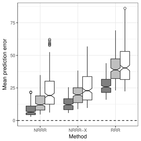
(a) Setting 1

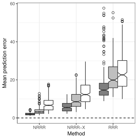
(b) Setting 2

Figure 2: Boxplots of MSFPE from 300 simulation runs. In each panel, each set of three boxplots for $\rho=0.1,0.5,0.9$ is showing in black, grey and white colors from left to right.

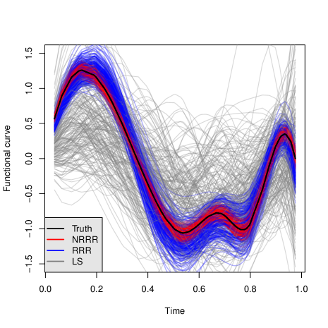
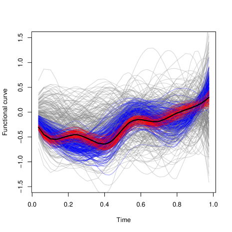
Figure 3: Comparison of the true curves and the predicted curves in two simulation runs under Setting 1 with $\mbox{SNR}=2$ and $\rho=0.5$.

6 Application to Adelaide Electricity Demand Data

Adelaide is the capital city of the state of South Australia. The city has a Mediterranean climate, with warm-dry summers and cool-mild winters. In summer time, the cooling mainly depends on air conditioning, which makes the electricity demand highly dependent on the weather conditions, and a large volatility in temperature throughout the day could make stable electricity supply challenging. Therefore, it is of great interest to understand the dependence and the predictive association between the electricity demand and the temperature, for facilitating the supply management of electricity (Magnano, 2007; Magnano et al., 2008; Fan and Hyndman, 2015). Here we apply NRRR to perform a multivariate functional regression analysis between daily half-hour electricity demand profiles for the 7 days of a week and the corresponding temperature profiles for the 7 days of the same week.

Half-hourly temperature records at two locations, Adelaide Kent town and Adelaide airport, are available between 7/6/1997 and 3/31/2007. Also available are the half-hourly electricity demand records of Adelaide for the same period. As such, for each day during the period, there are three observed functional curves, each with 48 half-hourly observations. As an illustration, Figure 4 plots the temperature and electricity demand profiles of all the Mondays from 7/6/1997 to 3/31/2007. Since our main focus is on studying the general association between the within-day demand and temperature trajectories in a week, we center the 48 discrete observations of each daily curve, to remove the between-day trend and seasonality of the data. Each week is then treated as a replication.

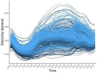
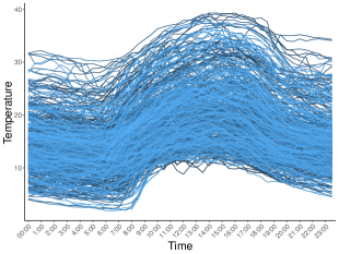
Figure 4: Adelaide electricity demand analysis: (a) electricity demand in Adelaide, (b) temperature in Kent town, and (c) temperature in the airport. Plotted are the half-hourly observed profiles for all Mondays.

After data pre-processing, we use the daily half-hour electricity demand as the functional multivariate response with $d=7$ (corresponding to 7 days in a week from Monday to Sunday), and as for the predictors, we consider two settings. In the first setting, we only use the half-hour temperature data from Kent as the multivariate functional predictors, so that $p=7$; in the second setting, we also include temperature data from the airport to make $p=14$. Not surprisingly, the two sets of temperature data are extremely highly correlated, so the second setting is meant to test for the behaviors of different methods in the presence of high collinearity. In either setting, the total sample size is $n=508$, equaling to the number of weeks in the study period. To leave sufficient flexibility in estimating the regression surface, we use B-spline with 30 degrees of freedom to convert the discrete observations to its integrated form according to (6).

First, we compare different methods using an out-of-sample random splitting procedure. Each time, we randomly select 400 samples as the training set and the remaining 108 samples as the test set. The model is fitted using the training data, and the relative mean squared prediction error (RMSPE) is then computed based on the test data,

$$\mbox{RMSPE}(\widehat{\bf y},{\bf y})=\frac{1}{n_{te}}\sum_{i=1}^{n_{te}}\frac{\int\|{\bf y}_{te,i}(t)-\widehat{\bf y}_{te,i}(t)\|^{2}dt}{\int\|{\bf y}_{te,i}(t)\|^{2}dt}.$$

The procedure is repeated 100 times, and the results are reported in Table 3. In both settings, NRRR and NRRS perform very well, and their predicted curves are able to account for about 74% of the total variation in the observed demand curves. The results show that there is a dramatic global dimension reduction of the functional predictors, as $r_{x}$ is estimated to be only $1$ most of the times. As $r_{y}$ is often close to the number of original functional responses, this indicates that each daily electricity demand curve has its own pattern, and thus there is not much room for a global dimension reduction. In contrast, RRR and RRS perform much worse in prediction, and RRR even fails completely in Setting 2. To visualize, Figure 5 plots some randomly selected observed and predicted curves under Setting 1; the superior performance of NRRR is apparent. These results clearly show the power and necessity of global dimension reduction, especially in the presence of high correlation among the functional predictors.

Table 3: Adelaide electricity demand analysis: out-of-sample performance of different methods. Reported are the means and standard deviations (in parenthesis) of RMSPE, $r$, $r_{x}$ and $r_{y}$ over 100 simulation runs.

	Methods	RRR	NRRR	RRS	NRRS
Setting 1	RMSPE	0.42 (0.04)	0.27 (0.02)	0.38 (0.03)	0.26 (0.02)
	$r$	1.53 (0.63)	4.06 (0.28)	3.60 (0.70)	4.09 (0.35)
	$r_{x}$		1.00 (0.00)		1.01 (0.10)
	$r_{y}$		5.70 (1.47)		5.73 (1.43)
Setting 2	RMSPE	1.08 (0.19)	0.26 (0.02)	0.55 (0.05)	0.26 (0.02)
	$r$	0.26 (0.44)	4.45 (0.89)	1.00 (0.00)	4.40 (0.80)
	$r_{x}$		1.00 (0.00)		1.01 (0.10)
	$r_{y}$		6.72 (0.57)		6.75 (0.52)

Figure 5: Adelaide electricity demand analysis: randomly selected examples of observed demand curves (in black) and out-of-sample predicted curves by RRR (in blue) and NRRR (in red).

We then use all data to fit a final NRRR model with only the temperature observations from Kent. The estimated rank values are $\widehat{r}=4$, $\widehat{r}_{x}=1$, and $\widehat{r}_{y}=5$. The estimated loading matrix for the predictors is $\widehat{\bf V}=(0.22,0.39,0.46,0.52,0.43,0.28,0.25)^{\rm T}.$ This shows that there is only one latent functional predictor that is driving the patterns of the electronic demands, and this factor can be roughly explained as the averaged daily temperature profile of the week. It appears that the days closer to the middle of the week load higher. On the response side, there is not much global reduction, as the estimated loading matrix $\widehat{{\bf U}}$ is of rank 5. To make sense of $\widehat{{\bf U}}$, it may be more convenient to examine the two basis vectors of its orthogonal complement, i.e., the first two singular vectors of ${\bf I}-\widehat{{\bf U}}\widehat{{\bf U}}^{\rm T}$, which give the latent response factors that are not related to the temperatures at all. While the first loading vector $(-0.52,0.36,0.28,0.25,-0.56,0.34,-0.18)^{\rm T}$ is hard to interpret, the second loading vector $(0.00,-0.68,0.73,0.00,-0.04,0.05,-0.04)^{\rm T}$ clearly indicates that the difference between the electronic demand profiles of Tuesday and Wednesday is mostly a noise process. In other words, the demand profiles of these two days are related to the temperature process in almost the same way.

Let $\widetilde{{\bf u}}_{k}$ be the $k$th row of $\widehat{{\bf U}}$. Then Model (4) shows that the estimated regression surface

$$\widetilde{c}_{k}(s,t)=\widetilde{{\bf u}}_{k}^{\rm T}({\bf I}_{\widehat{r}_{y}}\otimes{\boldsymbol{\Psi}}^{\rm T}(t))\widehat{{\bf A}}^{*}\widehat{{\bf B}}^{*\rm T}({\bf I}_{\widehat{r}_{x}}\otimes{\boldsymbol{\Phi}}(s)),\qquad k=1,\ldots,d,$$ (15)

would indicate how the response $y_{k}(t)$ is related to the latent predictor $\widehat{{\bf V}}^{\rm T}{\bf x}(s)$ over $s$ and $t$. In the context of this application, $\widetilde{c}_{k}(s,t)$ shows that how the electricity demand trajectory on the $k$th day of a week is related to the trajectory of the average temperature of the week. We therefore plot the heatmaps of these surfaces to visualize. Figure 6 displays the plots for Tuesday and Saturday. While the patterns of the association are hard to comprehend in general, some observations can be made. First, there are three association regimes throughout each day, i.e., night hours from about midnight to 7:30, daylight hours from about 7:30 to 18:00, and the rest hours from about 18:00 to midnight. This corresponds well with the general patterns of daily electricity demand, and the three regimes are separated by the “Morning ramp”, i.e., the transition from relatively lower loads to higher loads in the morning, and the peak load time around 18:00. Noticeably, the electricity demand in daylight hours is the least associated with the temperature. Another observation is that temperatures between about 19:00 to 20:30 and 23:00 to 00:00 in general have the largest effects on the electricity demand. This may be related to household and entertainment activities. Lastly, we observe that the association patterns on the workdays are similar to each other, and are slightly different from those on the weekends.

(a) Tuesday

(b) Saturday

Figure 6: Adelaide electricity demand analysis: heatmaps of estimated regression surfaces defined in (15).

7 Discussion

There are many research directions that stem from the proposed nested reduced-rank estimation framework. Our method can be extended to the historical functional regression, i.e., when $s$ and $t$ are both on the same domain such as time, it is required that ${\bf C}(s,t)=0$ for any $s>t$, so that the future dynamics of ${\bf x}(s)$ is not used in the modeling of the current or past dynamics of ${\bf y}(t)$. Another interesting direction is to consider sparse and low-rank estimation. For example, to enable the selection of the functional predictors, we could assume that ${\bf V}_{0}$ is a row-sparse matrix and utilize group-wise regularization such as group lasso in estimation. On the theoretical side, it is pressing to study the non-asymptotic behavior of our proposed estimator under reasonable conditions on the integrated design matrix originated from the functional setup. Last but not the least, we will further explore the nested reduced-rank structure, or even more generally, a multi-resolution reduced-rank structure in other statistical problems such as time series analysis and large-scale matrix denoising/approximation tasks.

Appendix

A: Proofs of Main Theoretical Results

Parameterization

Denote $\Omega$ as the parameter space of the set of matrices ${\bf C}\in\mathbb{R}^{J_{x}p\times J_{y}d}$ with a nested reduced-rank structure $({\bf I}_{J_{x}}\otimes{\bf V}){\bf B}{\bf A}^{\rm T}({\bf I}_{J_{y}}\otimes{\bf U}^{\rm T})$ with rank values $(r_{x},r_{y},r)$. This decomposition is not unique, e.g., with any comfortable and invertible matrices ${\bf Q}_{1},{\bf Q}_{2}$ and ${\bf Q}_{3}$, we can write

$${\bf C}= ({\bf I}_{J_{x}}\otimes{\bf V}){\bf B}{\bf A}^{\rm T}({\bf I}_{J_{y}}\otimes{\bf U}^{\rm T})$$

$$= [{\bf I}_{J_{x}}\otimes({\bf V}{\bf Q}_{1}^{-1})][({\bf I}_{J_{x}}\otimes{\bf Q}_{1}){\bf B}{\bf Q}_{2}^{\rm T}][{\bf Q}_{2}^{-\rm T}{\bf A}^{\rm T}({\bf I}_{J_{y}}\otimes{\bf Q}_{3}^{\rm T})][{\bf I}_{J_{y}}\otimes({\bf Q}_{3}^{-T}{\bf U}^{\rm T})].$$ (16)

We therefore consider a reparameterization of ${\bf C}$ in order to make its components identifiable and then characterize $\Omega$. Recall that ${\bf V}\in\mathbb{R}^{p\times r_{x}}$ is designed to capture the global low-dimensional structure in predictors and has rank $r_{x}$ ($\leq p$), then there must exists an invertible sub-matrix ${\bf V}_{L_{1},\cdot}\in\mathbb{R}^{r_{x}\times r_{x}}$ which consists of a set of linearly independent rows. Here $L_{1}=\{l_{1},l_{2},\ldots,l_{r_{x}}\}$ is the row index set. Take ${\bf Q}_{1}={\bf V}_{L_{1},\cdot}$ in (16) and we have $({\bf V}{\bf Q}_{1}^{-1})_{L_{1},\cdot}={\bf I}_{r_{x}}$. Similarly, for ${\bf U}$ we can let ${\bf Q}_{3}={\bf U}_{L_{3},\cdot}\in\mathbb{R}^{r_{y}\times r_{y}}$ such that $({\bf U}{\bf Q}_{3}^{-1})_{L_{3},\cdot}={\bf I}_{r_{y}}$ where $L_{3}$ is the required row index set. Now consider the term $({\bf I}_{J_{x}}\otimes{\bf Q}_{1}){\bf B}{\bf A}^{\rm T}({\bf I}_{J_{y}}\otimes{\bf Q}_{3}^{\rm T})\in\mathbb{R}^{J_{x}r_{x}\times J_{y}r_{y}}$, which has rank $r$; we can find an invertible sub-matrix ${\bf Q}_{2}\in\mathbb{R}^{r\times r}$ in $({\bf I}_{J_{y}}\otimes{\bf Q}_{3}){\bf A}$ to make $(({\bf I}_{J_{y}}\otimes{\bf Q}_{3}){\bf A}{\bf Q}_{2}^{-1})_{L_{2},\cdot}={\bf I}_{r}$. This shows that a nested low-rank matrix can always be reparameterized such that each of ${\bf V}$, ${\bf U}$, ${\bf A}$ is embedded with an identity sub-matrix. With such a representation, $\Omega$ admits a manifold structure that is a union of ${p\choose r_{x}}\times{d\choose r_{y}}\times{J_{y}r_{y}\choose r}$ many components, i.e.,

$$\Omega=\cup_{L_{1}\times L_{2}\times L_{3}\in\Pi}\Omega_{L_{1}\times L_{2}\times L_{3}}$$

where

$$\Omega_{L_{1}\times L_{2}\times L_{3}}= \{({\bf I}_{J_{x}}\otimes\check{\bf V})\check{\bf B}\check{\bf A}^{\rm T}({\bf I}_{J_{y}}\otimes\check{\bf U})^{\rm T}:\check{\bf V}\in\mathbb{R}^{p\times r_{x}}\ \text{with}\ \check{\bf V}_{L_{1},\cdot}={\bf I}_{r_{x}};\check{\bf B}\in\mathbb{R}^{(J_{x}r_{x})\times r};$$

$$\check{\bf A}\in\mathbb{R}^{(J_{y}r_{y})\times r}\ \text{with}\ \check{\bf A}_{L_{2},\cdot}={\bf I}_{r};\check{\bf U}\in\mathbb{R}^{d\times r_{y}}\ \text{with}\ \check{\bf U}_{L_{3},\cdot}={\bf I}_{r_{y}}\}$$

and $\Pi$ consists of all possible index sets $L_{1}\times L_{2}\times L_{3}$ with $L_{1}\subseteq\{1,\ldots,p\},L_{2}\subseteq\{1,\ldots,J_{y}r_{y}\}$ and $L_{3}\subseteq\{1,\ldots,d\}$.

Proof of Theorem 1

Proof.

Based on the above characterization of $\Omega$, we now construct a local neighborhood around the true coefficient matrix ${\bf C}_{0}$, in order to investigate the asymptotic behavior of the NRRR estimation. Suppose ${\bf C}_{0}\in\Omega_{L_{1}\times L_{2}\times L_{3}}$, where $L_{1},L_{2}$ and $L_{3}$ are three fixed index sets. Define $\check{\bf V}={\bf V}_{0}{\bf Q}_{1}^{-1}$, $\check{\bf U}={\bf U}_{0}{\bf Q}_{3}^{-1}$, $\check{\bf B}=({\bf I}_{J_{x}}\otimes{\bf Q}_{1}){\bf B}_{0}{\bf Q}_{2}^{\rm T}$ and $\check{\bf A}=({\bf I}_{J_{y}}\otimes{\bf Q}_{3}){\bf A}_{0}{\bf Q}_{2}^{-1}$ so that $\check{\bf V}_{L_{1},\cdot}={\bf I}_{r_{x}}$, $\check{\bf A}_{L_{2},\cdot}={\bf I}_{r}$ and $\check{\bf U}_{L_{3},\cdot}={\bf I}_{r_{y}}$. It can be verified that

$${\bf C}_{0} =({\bf I}_{J_{x}}\otimes{\bf V}_{0}){\bf B}_{0}{\bf A}_{0}^{\rm T}({\bf I}_{J_{y}}\otimes{\bf U}_{0}^{\rm T})$$

$$=[{\bf I}_{J_{x}}\otimes({\bf V}_{0}{\bf Q}_{1}^{-1})][({\bf I}_{J_{x}}\otimes{\bf Q}_{1}){\bf B}_{0}{\bf Q}_{2}^{\rm T}][{\bf Q}_{2}^{-\rm T}{\bf A}_{0}^{\rm T}({\bf I}_{J_{y}}\otimes{\bf Q}_{3}^{\rm T})][{\bf I}_{J_{y}}\otimes({\bf Q}_{3}^{-\rm T}{\bf U}_{0}^{\rm T})]$$

$$=({\bf I}_{J_{x}}\otimes\check{\bf V})\check{\bf B}\check{\bf A}^{\rm T}({\bf I}_{J_{y}}\otimes\check{\bf U}^{\rm T}).$$

A local neighborhood centered at ${\bf C}_{0}$ of radius $h>0$ is constructed as follows,

$$\mathcal{N}({\bf C}_{0},h)= \bigg{\{}\left[{\bf I}_{J_{x}}\otimes\left(\check{\bf V}+\frac{1}{\sqrt{n}}\check{\bf R}^{1}\right)\right]\left(\check{\bf B}+\frac{1}{\sqrt{n}}\check{\bf R}^{2}\right)\left(\check{\bf A}+\frac{1}{\sqrt{n}}\check{\bf R}^{3}\right)^{\rm T}\left[{\bf I}_{J_{y}}\otimes\left(\check{\bf U}+\frac{1}{\sqrt{n}}\check{\bf R}^{4}\right)\right]^{\rm T}:\bigg{.}$$

$$\check{\bf R}^{1}\in\mathbb{R}^{p\times r_{x}}\ \text{with}\ \check{\bf R}^{1}_{L_{1},\cdot}={\bf 0},\|\check{\bf R}^{1}\|_{F}\leq h;$$

$$\check{\bf R}^{2}\in\mathbb{R}^{(J_{x}r_{x})\times r},\|\check{\bf R}^{2}\|_{F}\leq h;$$

$$\check{\bf R}^{3}\in\mathbb{R}^{(J_{y}r_{y})\times r}\ \text{with}\ \check{\bf R}^{3}_{L_{2},\cdot}={\bf 0},\|\check{\bf R}^{3}\|_{F}\leq h;$$

$$\bigg{.}\check{\bf R}^{4}\in\mathbb{R}^{d\times r_{y}}\ \text{with}\ \check{\bf R}^{4}_{L_{3},\cdot}={\bf 0},\|\check{\bf R}^{4}\|_{F}\leq h\bigg{\}}.$$

The zero parts in perturbation matrices $\check{\bf R}^{1}$, $\check{\bf R}^{3}$ and $\check{\bf R}^{4}$ ensure that $\mathcal{N}({\bf C}_{0},h)\subseteq\Omega_{L_{1}\times L_{2}\times L_{3}}\subseteq\mathcal{N}({\bf C}_{0},\infty)$. Also note that we can equivalently express the neighborhood in terms of ${\bf V}_{0},{\bf B}_{0},{\bf A}_{0},{\bf U}_{0}$ as

$$\mathcal{N}({\bf C}_{0},h)= \bigg{\{}\left[{\bf I}_{J_{x}}\otimes\left({\bf V}_{0}+\frac{1}{\sqrt{n}}{\bf R}^{1}\right)\right]\left({\bf B}_{0}+\frac{1}{\sqrt{n}}{\bf R}^{2}\right)\left({\bf A}_{0}+\frac{1}{\sqrt{n}}{\bf R}^{3}\right)^{\rm T}\left[{\bf I}_{J_{y}}\otimes\left({\bf U}_{0}+\frac{1}{\sqrt{n}}{\bf R}^{4}\right)\right]^{\rm T}:\bigg{.}$$

$${\bf R}^{1}=\check{\bf R}^{1}{\bf Q}_{1}\in\mathbb{R}^{p\times r_{x}}\ \text{with}\ {\bf R}^{1}_{L_{1},\cdot}=\check{\bf R}^{1}_{L_{1},\cdot}={\bf 0},\|\check{\bf R}^{1}\|_{F}\leq h;$$

$${\bf R}^{2}=({\bf I}_{J_{x}}\otimes{\bf Q}_{1}^{-1})\check{\bf R}^{2}{\bf Q}_{2}^{\rm T}\in\mathbb{R}^{(J_{x}r_{x})\times r},\|\check{\bf R}^{2}\|_{F}\leq h;$$

$${\bf R}^{3}=({\bf I}_{J_{y}}\otimes{\bf Q}_{3}^{-1})\check{\bf R}^{3}{\bf Q}_{2}\in\mathbb{R}^{(J_{y}r_{y})\times r}\ \text{with}\ \check{\bf R}^{3}_{L_{2},\cdot}={\bf 0},\|\check{\bf R}^{3}\|_{F}\leq h;$$

$$\bigg{.}{\bf R}^{4}=\check{\bf R}^{4}{\bf Q}_{3}\in\mathbb{R}^{d\times r_{y}}\ \text{with}\ {\bf R}^{4}_{L_{3},\cdot}=\check{\bf R}^{4}_{L_{3},\cdot}={\bf 0},\|\check{\bf R}^{4}\|_{F}\leq h\bigg{\}}.$$

With the above setup, we now investigate the consistency of the NRRR estimation that minimizes the objective function

$${\bf Q}_{n}({\bf V},{\bf B},{\bf A},{\bf U})=\|{\bf Y}-{\bf X}({\bf I}_{J_{x}}\otimes{\bf V}){\bf B}{\bf A}^{\rm T}({\bf I}_{J_{y}}\otimes{\bf U}^{\rm T})\|_{F}^{2}.$$

We claim that for any given $\epsilon>0$, there exists a large enough constant $h$ such that

$$\mathbb{P}\bigg{\{}\inf_{\|\check{\bf R}^{1}\|_{F}=\|\check{\bf R}^{2}\|_{F}=\|\check{\bf R}^{3}\|_{F}=\|\check{\bf R}^{4}\|_{F}=h} {\bf Q}_{n}({\bf V}_{0}+\frac{1}{\sqrt{n}}{\bf R}^{1},{\bf B}_{0}+\frac{1}{\sqrt{n}}{\bf R}^{2},{\bf A}_{0}+\frac{1}{\sqrt{n}}{\bf R}^{3},{\bf U}_{0}+\frac{1}{\sqrt{n}}{\bf R}^{4})\bigg{.}$$

$$\bigg{.}>{\bf Q}_{n}({\bf V}_{0},{\bf B}_{0},{\bf A}_{0},{\bf U}_{0})\bigg{\}}\geq 1-\epsilon.$$ (17)

This statement implies that with probability at least $1-\epsilon$, there exists a local minimum $\widehat{\bf C}=({\bf I}_{J_{x}}\otimes\widehat{\bf V})\widehat{\bf B}\widehat{\bf A}^{\rm T}({\bf I}_{J_{y}}\otimes\widehat{\bf U}^{\rm T})$ in the interior of the ball $\mathcal{N}({\bf C}_{0},h)$ and it satisfies

$$\|(\widehat{\bf V}-{\bf V}_{0}){\bf Q}_{1}^{-1}\|_{F}=O_{p}(n^{-\frac{1}{2}}),$$

$$\|({\bf I}_{J_{x}}\otimes{\bf Q}_{1})(\widehat{\bf B}-{\bf B}_{0}){\bf Q}_{2}^{-\rm T}\|_{F}=O_{p}(n^{-\frac{1}{2}}),$$

$$\|({\bf I}_{J_{y}}\otimes{\bf Q}_{3})(\widehat{\bf A}-{\bf A}_{0}){\bf Q}_{2}^{-1}\|_{F}=O_{p}(n^{-\frac{1}{2}}),$$

$$\|(\widehat{\bf U}-{\bf U}_{0}){\bf Q}_{3}^{-1}\|_{F}=O_{p}(n^{-\frac{1}{2}}).$$

Then based on the fact $\|{\bf A}{\bf B}\|_{F}\leq\|{\bf A}\|_{F}\|{\bf B}\|_{F}$ for any two matrices ${\bf A}$ and ${\bf B}$, we have

$$\|(\widehat{\bf V}-{\bf V}_{0}){\bf Q}_{1}^{-1}\|_{F}\|{\bf Q}_{1}^{-1}\|_{F}^{-1}\leq\|\widehat{\bf V}-{\bf V}_{0}\|_{F}\leq\|(\widehat{\bf V}-{\bf V}_{0}){\bf Q}_{1}^{-1}\|_{F}\|{\bf Q}_{1}\|_{F}.$$

Thus with $\|{\bf Q}_{1}\|_{F}<\infty$ we obtain $\|\widehat{\bf V}-{\bf V}_{0}\|_{F}=O_{p}(n^{-\frac{1}{2}})$. Similarly, with $\|{\bf Q}_{2}\|_{F}<\infty$ and $\|{\bf Q}_{3}\|_{F}<\infty$ we can obtain $\|\widehat{\bf B}-{\bf B}_{0}\|_{F}=O_{p}(n^{-\frac{1}{2}})$, $\|\widehat{\bf A}-{\bf A}_{0}\|_{F}=O_{p}(n^{-\frac{1}{2}})$ and $\|\widehat{\bf U}-{\bf U}_{0}\|_{F}=O_{p}(n^{-\frac{1}{2}})$.

It remains to verify (Proof.). Let’s write

$$\left[{\bf I}_{J_{x}}\otimes\left({\bf V}_{0}+\frac{1}{\sqrt{n}}{\bf R}^{1}\right)\right]\left({\bf B}_{0}+\frac{1}{\sqrt{n}}{\bf R}^{2}\right)\left({\bf A}_{0}+\frac{1}{\sqrt{n}}{\bf R}^{3}\right)^{\rm T}\left[{\bf I}_{J_{y}}\otimes\left({\bf U}_{0}+\frac{1}{\sqrt{n}}{\bf R}^{4}\right)\right]^{\rm T}\in\mathcal{N}({\bf C}_{0},h)$$

as any perturbed matrix within $\mathcal{N}({\bf C}_{0},h)$ and define

$$\Psi_{n}({\bf R}^{1},{\bf R}^{2},{\bf R}^{3},{\bf R}^{4})= {\bf Q}_{n}({\bf V}_{0}+n^{-\frac{1}{2}}{\bf R}^{1},{\bf B}_{0}+n^{-\frac{1}{2}}{\bf R}^{2},{\bf A}_{0}+n^{-\frac{1}{2}}{\bf R}^{3},{\bf U}_{0}+n^{-\frac{1}{2}}{\bf R}^{4})$$

$$-{\bf Q}_{n}({\bf V}_{0},{\bf B}_{0},{\bf A}_{0},{\bf U}_{0}).$$

By some algebra, we get

$$\Psi_{n}({\bf R}^{1},{\bf R}^{2},{\bf R}^{3},{\bf R}^{4})=-{\bf Z}^{\rm T}\mbox{vec}\left(\frac{{\bf X}^{\rm T}{\bf E}}{\sqrt{n}}\right)+{\bf Z}^{\rm T}\left({\bf I}_{J_{y}d}\otimes\frac{{\bf X}^{\rm T}{\bf X}}{n}\right){\bf Z}+O_{p}(n^{-\frac{1}{2}})$$ (18)

where

$${\bf Z}= vec(({\bf I}_{J_{x}}\otimes{\bf R}^{1}){\bf B}_{0}{\bf A}_{0}^{\rm T}({\bf I}_{J_{y}}\otimes{\bf U}_{0}^{\rm T})+({\bf I}_{J_{x}}\otimes{\bf V}_{0}){\bf R}^{2}{\bf A}_{0}^{\rm T}({\bf I}_{J_{y}}\otimes{\bf U}_{0}^{\rm T})$$

$$+({\bf I}_{J_{x}}\otimes{\bf V}_{0}){\bf B}_{0}{\bf R}^{3\rm T}({\bf I}_{J_{y}}\otimes{\bf U}_{0}^{\rm T})+({\bf I}_{J_{x}}\otimes{\bf V}_{0}){\bf B}_{0}{\bf A}_{0}^{\rm T}({\bf I}_{J_{y}}\otimes{\bf R}^{4\rm T})).$$

Because

$$\mbox{vec}\left(\frac{1}{\sqrt{n}}{\bf X}^{\rm T}{\bf E}\right)\rightarrow^{d}N({\bf 0},{\bf\Sigma}\otimes{\boldsymbol{\Gamma}})$$

and

$${\bf I}_{J_{y}d}\otimes\frac{{\bf X}^{\rm T}{\bf X}}{n}\rightarrow{\bf I}_{J_{y}d}\otimes{\boldsymbol{\Gamma}},$$

it suffices to show that for a large enough $h$, denoted as $h_{n}^{*}$, $\|{\bf Z}\|^{2}$ dominates $\|{\bf Z}\|$ for $({\bf R}^{1},{\bf R}^{2},{\bf R}^{3},{\bf R}^{4})$ with $\|\check{\bf R}^{1}\|_{F}=\|\check{\bf R}^{2}\|_{F}=\|\check{\bf R}^{3}\|_{F}=\|\check{\bf R}^{4}\|_{F}=h$. For simplicity, write ${\bf Z}=\mbox{vec}({\bf P}_{1}+{\bf P}_{1}+{\bf P}_{3}+{\bf P}_{4})$ where

$${\bf P}_{1}=({\bf I}_{J_{x}}\otimes{\bf R}^{1}){\bf B}_{0}{\bf A}_{0}^{\rm T}({\bf I}_{J_{y}}\otimes{\bf U}_{0}^{\rm T}),$$

$${\bf P}_{2}=({\bf I}_{J_{x}}\otimes{\bf V}_{0}){\bf R}^{2}{\bf A}_{0}^{\rm T}({\bf I}_{J_{y}}\otimes{\bf U}_{0}^{\rm T}),$$

$${\bf P}_{3}=({\bf I}_{J_{x}}\otimes{\bf V}_{0}){\bf B}_{0}{\bf R}^{3\rm T}({\bf I}_{J_{y}}\otimes{\bf U}_{0}^{\rm T}),$$

$${\bf P}_{4}=({\bf I}_{J_{x}}\otimes{\bf V}_{0}){\bf B}_{0}{\bf A}_{0}^{\rm T}({\bf I}_{J_{y}}\otimes{\bf R}^{4\rm T}),$$

and also write

$${\bf B}_{0}=({\bf B}_{01}^{\rm T},\cdots,{\bf B}_{0J_{x}}^{\rm T})^{\rm T},\quad{\bf B}_{0i}\in\mathbb{R}^{r_{x}\times r},\quad i=1,\ldots,J_{x}$$

$${\bf A}_{0}=({\bf A}_{01}^{\rm T},\cdots,{\bf A}_{0J_{y}}^{\rm T})^{\rm T},\quad{\bf A}_{0j}\in\mathbb{R}^{r_{y}\times r},\quad j=1,\ldots,J_{y}$$

$$\check{\bf R}^{2}=(\check{\bf R}^{2\rm T}_{1},\ldots,\check{\bf R}^{2\rm T}_{J_{x}})^{\rm T},\quad\check{\bf R}^{2}_{i}\in\mathbb{R}^{r_{x}\times r},\quad i=1,\ldots,J_{x}$$

$$\check{\bf R}^{3}=(\check{\bf R}^{3\rm T}_{1},\ldots,\check{\bf R}^{3\rm T}_{J_{y}})^{\rm T},\quad\check{\bf R}^{3}_{j}\in\mathbb{R}^{r_{y}\times r},\quad j=1,\ldots,J_{y}.$$

Let’s first consider

$${\bf P}_{1}=\begin{pmatrix}{\bf R}^{1}{\bf B}_{01}{\bf A}^{\rm T}_{01}{\bf U}_{0}^{\rm T}&\cdots&{\bf R}^{1}{\bf B}_{01}{\bf A}^{\rm T}_{0J_{y}}{\bf U}_{0}^{\rm T}\\ \vdots&\ddots&\vdots\\ {\bf R}^{1}{\bf B}_{0J_{x}}{\bf A}^{\rm T}_{01}{\bf U}_{0}^{\rm T}&\cdots&{\bf R}^{1}{\bf B}_{0J_{x}}{\bf A}^{\rm T}_{0J_{y}}{\bf U}_{0}^{\rm T}\end{pmatrix},$$

where each block ${\bf R}^{1}{\bf B}_{0i}{\bf A}^{\rm T}_{0j}{\bf U}_{0}^{\rm T}\in\mathbb{R}^{p\times q}$ for $i=1,\ldots,J_{x},\ j=1,\ldots,J_{y}$. Recall that ${\bf R}^{1}_{L_{1},\cdot}={\bf 0}$, thus we have $({\bf R}^{1}{\bf B}_{0i}{\bf A}^{\rm T}_{0j}{\bf U}_{0}^{\rm T})_{L_{1},\cdot}={\bf 0}$. Without loss of generality, we assume $L_{1}=\{1,\ldots,r_{x}\}$. Then, if we write ${\bf P}_{1}=({\bf P}_{11}^{\rm T},\ldots,{\bf P}_{1J_{x}}^{\rm T})^{\rm T}$ with ${\bf P}_{1i}\in\mathbb{R}^{p\times(J_{y}d)},i=1,\ldots,J_{x}$, the first $r_{x}$ rows for each ${\bf P}_{1i}$ are zero vectors.

Next we deal with ${\bf P}_{4}$ which can be written as

$${\bf P}_{4}=\begin{pmatrix}{\bf V}_{0}{\bf B}_{01}{\bf A}^{\rm T}_{01}{\bf R}^{4\rm T}&\cdots&{\bf V}_{0}{\bf B}_{01}{\bf A}^{\rm T}_{0J_{y}}{\bf R}^{4\rm T}\\ \vdots&\ddots&\vdots\\ {\bf V}_{0}{\bf B}_{0J_{x}}{\bf A}^{\rm T}_{01}{\bf R}^{4\rm T}&\cdots&{\bf V}_{0}{\bf B}_{0J_{x}}{\bf A}^{\rm T}_{0J_{y}}{\bf R}^{4\rm T}\end{pmatrix},$$

where each block ${\bf V}_{0}{\bf B}_{0i}{\bf A}^{\rm T}_{0j}{\bf R}^{4\rm T}\in\mathbb{R}^{p\times q}$ for $i=1,\ldots,J_{x},\ j=1,\ldots,J_{y}$. With ${\bf R}^{4}_{L_{3},\cdot}={\bf 0}$ we have $({\bf V}_{0}{\bf B}_{0i}{\bf A}^{\rm T}_{0j}R^{4\rm T})_{\cdot,L_{3}}={\bf 0}$. Without loss of generality, we assume $L_{3}=\{1,\ldots,r_{y}\}$. If we write ${\bf P}_{4}=({\bf P}_{41},\ldots,{\bf P}_{4J_{y}})$ with ${\bf P}_{4j}\in\mathbb{R}^{(J_{x}p)\times d},j=1,\ldots,J_{y}$, the first $r_{y}$ columns for each ${\bf P}_{4j}$ are zero vectors. To summarize, for each block ${\bf R}^{1}{\bf B}_{0i}{\bf A}^{\rm T}_{0j}{\bf U}_{0}^{\rm T}+{\bf V}_{0}{\bf B}_{0i}{\bf A}^{\rm T}_{0j}{\bf R}^{4\rm T}$ in ${\bf P}_{1}+{\bf P}_{4}$, the left-upper sub-matrix is a zero matrix of dimension $r_{x}\times r_{y}$.

Then we consider

$${\bf P}_{2} =({\bf I}_{J_{x}}\otimes{\bf V}_{0}){\bf R}^{2}{\bf A}_{0}^{\rm T}({\bf I}_{J_{y}}\otimes{\bf U}_{0}^{\rm T})$$

$$=({\bf I}_{J_{x}}\otimes\check{\bf V})\check{\bf R}^{2}\check{\bf A}^{\rm T}({\bf I}_{J_{y}}\otimes\check{\bf U}^{\rm T})$$

$$=\begin{pmatrix}\check{\bf V}\check{\bf R}^{2}_{1}\check{\bf A}^{\rm T}_{1}\check{\bf U}^{\rm T}&\cdots&\check{\bf V}\check{\bf R}^{2}_{1}\check{\bf A}^{\rm T}_{J_{y}}\check{\bf U}^{\rm T}\\ \vdots&\ddots&\vdots\\ \check{\bf V}\check{\bf R}^{2}_{J_{x}}\check{\bf A}^{\rm T}_{1}\check{\bf U}^{\rm T}&\cdots&\check{\bf V}\check{\bf R}^{2}_{J_{x}}\check{\bf A}^{\rm T}_{J_{y}}\check{\bf U}^{\rm T}\end{pmatrix}.$$

For each block $\check{\bf V}\check{\bf R}^{2}_{i}\check{\bf A}^{\rm T}_{j}\check{\bf U}^{\rm T}\in\mathbb{R}^{p\times d}$, we have $(\check{\bf V}\check{\bf R}^{2}_{i}\check{\bf A}^{\rm T}_{j}\check{\bf U}^{\rm T})_{L_{1},L_{3}}=\check{\bf R}^{2}_{i}\check{\bf A}^{\rm T}_{j}\in\mathbb{R}^{r_{x}\times r_{y}}$ because $\check{\bf V}_{L_{1},\cdot}={\bf I}_{r_{x}}$ and $\check{\bf U}_{L_{3},\cdot}={\bf I}_{r_{y}}$. Similarly, we have

$${\bf P}_{3} =({\bf I}_{J_{x}}\otimes\check{\bf V})\check{\bf B}\check{\bf R}^{3\rm T}({\bf I}_{J_{y}}\otimes\check{\bf U}^{\rm T})$$

$$=\begin{pmatrix}\check{\bf V}\check{\bf B}_{1}\check{\bf R}^{3\rm T}_{1}\check{\bf U}^{\rm T}&\cdots&\check{\bf V}\check{\bf B}_{1}\check{\bf R}^{3\rm T}_{J_{y}}\check{\bf U}^{\rm T}\\ \vdots&\ddots&\vdots\\ \check{\bf V}\check{\bf B}_{J_{x}}\check{\bf R}^{3\rm T}_{1}\check{\bf U}^{\rm T}&\cdots&\check{\bf V}\check{\bf B}_{J_{x}}\check{\bf R}^{3\rm T}_{J_{y}}\check{\bf U}^{\rm T}\end{pmatrix}$$

where each block $\check{\bf V}\check{\bf B}_{i}\check{\bf R}^{3\rm T}_{j}\check{\bf U}^{\rm T}\in\mathbb{R}^{p\times d}$ and $(\check{\bf V}\check{\bf B}_{i}\check{\bf R}^{3\rm T}_{j}\check{\bf U}^{\rm T})_{L_{1},L_{3}}=\check{\bf B}_{i}\check{\bf R}^{3\rm T}_{j}\in\mathbb{R}^{r_{x}\times r_{y}}$. Thus, if we extract the left upper sub-matrix which has dimension $r_{x}\times r_{y}$ from all blocks in ${\bf P}_{1}+{\bf P}_{2}+{\bf P}_{3}+{\bf P}_{4}$ and put them together, we can obtain a matrix

$$\begin{pmatrix}\check{\bf R}^{2}_{1}\check{\bf A}^{\rm T}_{1}+\check{\bf B}_{1}\check{\bf R}^{3\rm T}_{1}&\cdots&\check{\bf R}^{2}_{1}\check{\bf A}^{\rm T}_{J_{y}}+\check{\bf B}_{1}\check{\bf R}^{3\rm T}_{J_{y}}\\ \vdots&\ddots&\vdots\\ \check{\bf R}^{2}_{J_{x}}\check{\bf A}^{\rm T}_{1}+\check{\bf B}_{J_{x}}\check{\bf R}^{3\rm T}_{1}&\cdots&\check{\bf R}^{2}_{J_{x}}\check{\bf A}^{\rm T}_{J_{y}}+\check{\bf B}_{J_{x}}\check{R}^{3\rm T}_{J_{y}}\end{pmatrix}=\check{\bf R}^{2}\check{\bf A}^{\rm T}+\check{\bf B}\check{\bf R}^{3\rm T}.$$

From $\check{\bf R}^{3}_{L_{2},\cdot}={\bf 0}$, we have $(\check{\bf B}\check{\bf R}^{3\rm T})_{\cdot,L_{2}}={\bf 0}$. And from $\check{\bf A}_{L_{2},\cdot}={\bf I}_{r}$, we have $(\check{\bf R}^{2}\check{\bf A}^{\rm T})_{\cdot,L_{2}}=\check{\bf R}^{2}$. It leads to $(\check{\bf B}\check{\bf R}^{3\rm T}+\check{\bf R}^{2}\check{\bf A}^{\rm T})_{\cdot,L_{2}}=\check{\bf R}^{2}$ and $\|(\check{\bf B}\check{\bf R}^{3\rm T}+\check{\bf R}^{2}\check{\bf A}^{\rm T})_{\cdot,L_{2}}\|_{F}^{2}=\|\check{\bf R}^{2}\|_{F}^{2}=h^{2}$. Recall that $(\check{\bf B}\check{\bf R}^{3\rm T}+\check{\bf R}^{2}\check{\bf A}^{\rm T})_{\cdot,L_{2}}$ is a sub-matrix in ${\bf P}_{1}+{\bf P}_{2}+{\bf P}_{3}+{\bf P}_{4}$. Then with

$$\|{\bf Z}\|^{2}=\|{\bf P}_{1}+{\bf P}_{2}+{\bf P}_{3}+{\bf P}_{4}\|_{F}^{2}=h^{2}\left(1+f\left(\frac{\check{R}^{1}}{h},\frac{\check{R}^{2}}{h},\frac{\check{R}^{3}}{h},\frac{\check{R}^{4}}{h}\right)\right)\geq(k+1)h^{2},$$

where $f()$ is a non-negative, continuous function which attains its minimum value $k>0$ over the unit sphere $\{(\check{\bf R}^{1},\check{\bf R}^{2},\check{\bf R}^{3},\check{\bf R}^{4}):\|\check{\bf R}^{1}\|_{F}=1,\|\check{\bf R}^{2}\|_{F}=1,\|\check{\bf R}^{3}\|_{F}=1,\|\check{\bf R}^{4}\|_{F}=1;\check{\bf R}^{1}_{L_{1},\cdot}={\bf 0},\check{\bf R}^{3}_{L_{2},\cdot}={\bf 0},\check{\bf R}^{4}_{L_{3},\cdot}={\bf 0}\}$. We have verified the existence of $h_{n}^{*}$ due to the fact that $\|{\bf Z}\|$ is $O_{p}(h)$ uniformly. This completes the proof. ∎

Proof of Theorem 2

Proof.

By the definition of $\widehat{\bf C}$, we have

$$\|{\bf Y}-{\bf X}\widehat{\bf C}\|_{F}^{2}\leq\|{\bf Y}-\mathbf{XC}_{0}\|_{F}^{2},$$

which leads to

$$\|{\bf X}(\widehat{\bf C}-{\bf C}_{0})^{\rm T}\|_{F}^{2}\leq 2\langle{\bf E},{\bf X}(\widehat{\bf C}-{\bf C}_{0})^{\rm T}\rangle_{F},$$ (19)

where $\langle{\bf C},{\bf D}\rangle_{F}=\text{tr}({\bf C}^{\rm T}{\bf D})$. Furthermore,

$$\langle{\bf E},{\bf X}(\widehat{\bf C}-{\bf C}_{0})^{\rm T}\rangle_{F}=\langle\mathcal{P}{\bf E},{\bf X}(\widehat{\bf C}-{\bf C}_{0})^{\rm T}\rangle_{F},$$ (20)

where $\mathcal{P}={\bf X}\left({\bf X}^{\rm T}{\bf X}\right)^{-}{\bf X}^{\rm T}$ denotes the projection matrix onto the column space of ${\bf X}$. Let $d_{j}(\cdot)$ denote the $j^{\mbox{th}}$ largest singular value of the enclosed matrix. Then we have $\langle{\bf C},{\bf D}\rangle_{F}\leq d_{1}({\bf C})\|{\bf D}\|_{*}$, where $\|{\bf D}\|_{*}=\sum\nolimits_{j}d_{j}({\bf D})$ denotes the nuclear norm of ${\bf D}$. It follows that

$$\langle\mathcal{P}{\bf E},{\bf X}(\widehat{\bf C}-{\bf C}_{0})^{\rm T}\rangle_{F} \leq d_{1}(\mathcal{P}{\bf E})\|{\bf X}(\widehat{\bf C}-{\bf C}_{0})^{\rm T}\|_{*}$$ (21)

$$\leq d_{1}(\mathcal{P}{\bf E})\sqrt{2r}\|{\bf X}(\widehat{\bf C}-{\bf C}_{0})^{\rm T}\|_{F}.$$

Therefore, by (19) (20), and (21), we have

$$\|{\bf X}(\widehat{\bf C}-{\bf C}_{0})^{\rm T}\|_{F}\leq 2d_{1}(\mathcal{P}{\bf E})\sqrt{2r}.$$

By Lemma 3 in Bunea et al. (2011), we have

$$\mathbb{E}\left\{d_{1}(\mathcal{P}{\bf E})\right\}\leq\sigma\left(\sqrt{r({\bf X})}+\sqrt{dJ_{y}}\right)$$

and

$$\mathbb{P}\left\{d_{1}(\mathcal{P}{\bf E})\geq\mathbb{E}[d_{1}(\mathcal{P}{\bf E})]+\sigma\theta\left(\sqrt{r({\bf X})}+\sqrt{dJ_{y}}\right)\right\}\leq\exp\left\{-\frac{\theta^{2}}{2}(r({\bf X})+dJ_{y})\right\}$$

where $\theta$ is a positive constant. Therefore, $\|{\bf X}(\widehat{\bf C}-{\bf C}_{0})^{\rm T}\|_{F}=O_{p}\left(r^{1/2}(r({\bf X})+dJ_{y})^{1/2}\right)$ with probability at least $1-\exp\left\{-\theta^{2}(r({\bf X})+dJ_{y})/2\right\}$. The second result follows directly.

∎

B: Additional Simulation Results

Additional Simulation Results from BIC Tuning

We present the results on estimating $r$, $r_{x}$ and $r_{y}$ in this part. For methods with nested reduced-rank structure, BIC is exploited to select ranks.

Table 4: Simulation results for Setting 1 with true rank $r=5$. The mean and the percentage of matching with the true rank (in parenthesis) of rank estimation over 300 simulation runs are presented.

	$\rho$	NRRR	NRRR-X	RRR	RRS	NRRS
	0.1	3.58 (0.09)	2.46 (0.00)	1.80 (0.00)	4.15 (0.28)	4.02 (0.22)
SNR=1	0.5	3.17 (0.02)	2.24 (0.00)	1.65 (0.00)	3.95 (0.19)	3.51 (0.06)
	0.9	2.13 (0.00)	1.66 (0.00)	1.55 (0.00)	3.30 (0.03)	2.22 (0.00)
	0.1	4.88 (0.88)	4.37 (0.44)	3.65 (0.11)	4.91 (0.91)	4.91 (0.91)
SNR=2	0.5	4.71 (0.72)	4.01 (0.19)	3.40 (0.04)	4.80 (0.80)	4.82 (0.82)
	0.9	3.72 (0.09)	3.05 (0.00)	2.69 (0.00)	4.16 (0.31)	3.92 (0.16)
	0.1	5.00 (1.00)	4.97 (0.97)	4.88 (0.89)	4.99 (0.99)	5.00 (1.00)
SNR=4	0.5	5.00 (1.00)	4.90 (0.90)	4.66 (0.68)	4.99 (0.99)	5.00 (1.00)
	0.9	4.74 (0.73)	4.22 (0.33)	3.72 (0.12)	4.83 (0.84)	4.73 (0.74)

Table 5: Simulation results for Setting 2 with true rank $r=3$. The mean and the percentage of matching with the true rank (in parenthesis) of rank estimation over 300 simulation runs are presented.

	$\rho$	NRRR	NRRR-X	RRR	RRS	NRRS
	0.1	2.99 (0.99)	2.37 (0.40)	2.31 (0.58)	2.91 (0.91)	2.99 (0.99)
SNR=1	0.5	2.94 (0.94)	2.20 (0.29)	2.33 (0.47)	2.83 (0.83)	2.98 (0.98)
	0.9	2.51 (0.54)	1.89 (0.08)	2.12 (0.21)	2.64 (0.64)	2.71 (0.73)
	0.1	3.00 (1.00)	2.97 (0.97)	2.62 (0.87)	3.09 (0.94)	3.00 (1.00)
SNR=2	0.5	3.00 (1.00)	2.93 (0.93)	2.77 (0.89)	3.02 (0.92)	3.00 (1.00)
	0.9	2.98 (0.98)	2.72 (0.72)	2.77 (0.77)	3.02 (0.96)	3.00 (1.00)
	0.1	3.00 (1.00)	3.00 (1.00)	2.67 (0.89)	3.13 (0.93)	3.00 (1.00)
SNR=4	0.5	3.00 (1.00)	3.00 (1.00)	2.81 (0.93)	3.15 (0.95)	3.00 (1.00)
	0.9	3.00 (1.00)	2.97 (0.97)	2.96 (0.96)	3.00 (0.98)	3.00 (1.00)

Table 6: Simulation results for Setting 1 with true rank $r_{x}=3$. The mean and the percentage of matching with the true rank (in parenthesis) of $r_{x}$ estimation over 300 simulation runs are presented.

	$\rho$	NRRR	NRRR-X	NRRS
	0.1	2.63 (0.64)	2.62 (0.63)	2.75 (0.77)
SNR=1	0.5	2.41 (0.49)	2.40 (0.47)	2.50 (0.54)
	0.9	1.75 (0.13)	1.77 (0.13)	1.85 (0.19)
	0.1	3.00 (1.00)	3.00 (1.00)	3.00 (1.00)
SNR=2	0.5	3.00 (1.00)	3.00 (1.00)	3.00 (1.00)
	0.9	2.88 (0.87)	2.85 (0.84)	2.90 (0.90)
	0.1	3.00 (1.00)	3.00 (1.00)	3.00 (1.00)
SNR=4	0.5	3.00 (1.00)	3.00 (1.00)	3.00 (1.00)
	0.9	3.01 (0.99)	3.01 (0.99)	3.00 (1.00)

Table 7: Simulation results for Setting 2 with true rank $r_{x}=3$. The mean and the percentage of matching with the true rank (in parenthesis) of $r_{x}$ estimation over 300 simulation runs are presented.

	$\rho$	NRRR	NRRR-X	NRRS
	0.1	2.93 (0.93)	2.90 (0.90)	2.98 (0.88)
SNR=1	0.5	2.88 (0.89)	2.87 (0.88)	2.92 (0.91)
	0.9	2.44 (0.49)	2.44 (0.49)	2.55 (0.59)
	0.1	2.94 (0.94)	2.94 (0.94)	3.24 (0.78)
SNR=2	0.5	2.94 (0.94)	2.96 (0.96)	3.14 (0.86)
	0.9	2.98 (0.96)	2.99 (0.97)	3.09 (0.89)
	0.1	2.97 (0.96)	2.98 (0.98)	3.62 (0.85)
SNR=4	0.5	2.97 (0.97)	2.96 (0.97)	3.21 (0.93)
	0.9	3.00 (1.00)	3.00 (1.00)	3.09 (0.93)

Table 8: Simulation results for Setting 1 with true rank $r_{y}=3$. The mean and the percentage of matching with the true rank (in parenthesis) of $r_{y}$ estimation over 300 simulation runs are presented.

	$\rho$	NRRR	NRRS
	0.1	2.92 (0.92)	2.97 (0.97)
SNR=1	0.5	2.95 (0.95)	2.99 (0.99)
	0.9	2.95 (0.95)	2.98 (0.98)
	0.1	3.00 (1.00)	3.00 (1.00)
SNR=2	0.5	3.00 (1.00)	3.00 (1.00)
	0.9	3.01 (0.99)	3.00 (1.00)
	0.1	3.00 (1.00)	3.00 (1.00)
SNR=4	0.5	3.00 (1.00)	3.00 (1.00)
	0.9	3.00 (1.00)	3.00 (1.00)

Table 9: Simulation results for Setting 2 with true rank $r_{y}=3$. The mean and the percentage of matching with the true rank (in parenthesis) of $r_{y}$ estimation over 300 simulation runs are presented.

	$\rho$	NRRR	NRRS
	0.1	2.99 (0.99)	2.99 (0.99)
SNR=1	0.5	3.00 (1.00)	3.00 (1.00)
	0.9	3.00 (0.99)	3.00 (1.00)
	0.1	2.99 (0.99)	3.00 (1.00)
SNR=2	0.5	3.00 (1.00)	3.00 (1.00)
	0.9	3.00 (1.00)	3.00 (1.00)
	0.1	3.00 (1.00)	3.00 (1.00)
SNR=4	0.5	3.00 (1.00)	3.00 (1.00)
	0.9	3.00 (1.00)	3.00 (1.00)

Simulation Results from Cross Validation Tuning

We present simulation results under Setting 1 with all the ranks selected by 10-fold cross validation. Results of MSPE and MSFPE displayed here are the trimmed version with the smallest and the largest 20 observations deleted from 300 simulation runs.

Table 10: Simulation results for Setting 1. The trimmed means and standard deviations (in parenthesis) of MSPE are presented. To improve presentation, all values are multiplied by 10.

	$\rho$	NRRR	NRRR-X	RRR	RRS	NRRS
	0.1	11.05 (2.54)	11.42 (2.61)	14.67 (3.24)	11.52 (2.56)	10.80 (2.46)
SNR=1	0.5	17.34 (4.30)	17.84 (4.37)	22.40 (5.33)	17.45 (4.14)	16.76 (4.06)
	0.9	26.05 (8.72)	26.37 (8.74)	30.28 (9.51)	24.39 (7.79)	24.30 (8.03)
	0.1	2.72 (0.51)	2.81 (0.52)	3.91 (0.75)	3.12 (0.55)	2.81 (0.51)
SNR=2	0.5	4.07 (0.91)	4.21 (0.95)	5.78 (1.29)	4.48 (0.97)	4.12 (0.90)
	0.9	6.05 (1.98)	6.23 (2.03)	8.00 (2.55)	6.20 (1.96)	5.89 (1.88)
	0.1	0.66 (0.14)	0.68 (0.14)	0.93 (0.20)	0.96 (0.19)	0.77 (0.17)
SNR=4	0.5	1.04 (0.24)	1.08 (0.25)	1.46 (0.34)	1.31 (0.26)	1.15 (0.24)
	0.9	1.50 (0.48)	1.56 (0.50)	2.10 (0.66)	1.67 (0.49)	1.57 (0.47)

Table 11: Simulation results for Setting 1 with true rank $r=5$. The mean and the percentage of matching with the true rank (in parenthesis) of rank estimation over 300 simulation runs are presented.

	$\rho$	NRRR	NRRR-X	RRR	RRS	NRRS
	0.1	4.73 (0.75)	4.20 (0.36)	1.75 (0.00)	4.12 (0.26)	4.96 (0.85)
SNR=1	0.5	4.36 (0.52)	3.80 (0.18)	1.70 (0.00)	3.96 (0.19)	4.88 (0.74)
	0.9	2.81 (0.06)	2.40 (0.01)	1.53 (0.00)	3.29 (0.02)	4.39 (0.33)
	0.1	5.00 (1.00)	4.96 (0.96)	3.68 (0.12)	4.91 (0.91)	5.06 (0.94)
SNR=2	0.5	4.99 (0.98)	4.91 (0.91)	3.48 (0.04)	4.83 (0.83)	5.07 (0.94)
	0.9	4.63 (0.62)	4.17 (0.36)	2.70 (0.00)	4.26 (0.38)	5.02 (0.80)
	0.1	5.00 (1.00)	5.00 (1.00)	4.84 (0.86)	4.97 (0.97)	5.03 (0.98)
SNR=4	0.5	5.00 (1.00)	5.00 (1.00)	4.76 (0.76)	5.00 (1.00)	5.04 (0.96)
	0.9	5.00 (0.93)	4.85 (0.85)	3.70 (0.11)	4.83 (0.83)	5.12 (0.89)

Table 12: Simulation results for Setting 1 with true rank $r_{x}=3$. The mean and the percentage of matching with the true rank (in parenthesis) of $r_{x}$ estimation over 300 simulation runs are presented.

	$\rho$	NRRR	NRRR-X	NRRS
	0.1	2.85 (0.84)	2.85 (0.84)	3.05 (0.82)
SNR=1	0.5	2.67 (0.68)	2.67 (0.68)	3.08 (0.72)
	0.9	1.97 (0.21)	1.97 (0.21)	3.22 (0.41)
	0.1	3.00 (1.00)	3.00 (1.00)	3.00 (1.00)
SNR=2	0.5	3.00 (1.00)	3.00 (1.00)	3.02 (0.99)
	0.9	2.94 (0.86)	2.94 (0.86)	3.06 (0.93)
	0.1	3.00 (1.00)	3.00 (1.00)	3.00 (1.00)
SNR=4	0.5	3.00 (1.00)	3.00 (1.00)	3.00 (1.00)
	0.9	3.06 (0.94)	3.06 (0.94)	3.01 (0.99)

Table 13: Simulation results for Setting 1 with true rank $r_{y}=3$. The mean and the percentage of matching with the true rank (in parenthesis) of $r_{y}$ estimation over 300 simulation runs are presented.

	$\rho$	NRRR	NRRS
	0.1	3.17 (0.92)	3.04 (0.95)
SNR=1	0.5	3.15 (0.92)	3.05 (0.95)
	0.9	3.12 (0.93)	3.05 (0.95)
	0.1	3.01 (0.99)	3.03 (0.98)
SNR=2	0.5	3.00 (1.00)	3.01 (0.99)
	0.9	3.05 (0.95)	3.04 (0.96)
	0.1	3.00 (1.00)	3.01 (0.99)
SNR=4	0.5	3.00 (1.00)	3.01 (0.99)
	0.9	3.01 (0.99)	3.01 (0.99)

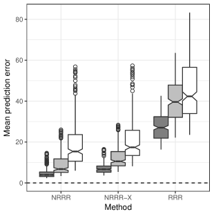
(a) SNR = 1

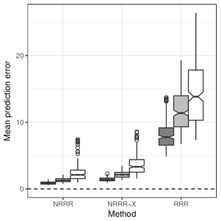
(b) SNR = 2

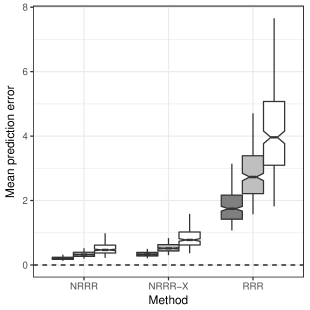
(c) SNR = 4

Figure 7: Boxplots of MSFPE from 300 simulation runs. From left to right are three plots with SNR being 1, 2, and 4. In each panel, each set of three boxplots for $\rho=0.1,0.5,0.9$ is showing in black, grey and white colors from left to right.

References

• Bunea et al. (2011) Bunea, F., She, Y., and Wegkamp, M. H. (2011), “Optimal Selection of Reduced Rank Estimators of High-Dimensional Matrices,” The Annals of Statistics, 39, 1282–1309.
• Cardot et al. (1999) Cardot, H., Ferraty, F., and Sarda, P. (1999), “Functional Linear Model,” Statistics & Probability Letters, 45, 11–22.
• Cardot et al. (2003) — (2003), “Spline Estimators for the Functional Linear Model,” Statistica Sinica, 13, 571–591.
• Chen et al. (2012) Chen, K., Chan, K.-S., and Stenseth, N. C. (2012), “Reduced Rank Stochastic Regression with a Sparse Singular Value Decomposition,” Journal of the Royal Statistical Society: Series B (Statistical Methodology), 74, 203–221.
• Chen et al. (2013) Chen, K., Dong, H., and Chan, K.-S. (2013), “Reduced Rank Regression via Adaptive Nuclear Norm Penalization,” Biometrika, 100, 901–920.
• Chiou et al. (2003) Chiou, J.-M., Muller, H.-G., and Wang, J.-L. (2003), “Functional Quasi-Likelihood Regression Models with Smooth Random Effects,” Journal of the Royal Statistical Society: Series B (Statistical Methodology), 65, 405–423.
• Chiou et al. (2016) Chiou, J.-M., Yang, Y.-F., and Chen, Y.-T. (2016), “Multivariate Functional Linear Regression and Prediction,” Journal of Multivariate Analysis, 146, 301–312.
• Ebaid (2008) Ebaid, R. (2008), “Reduced-Rank Regression of Functional Data,” Ph.D. thesis, Temple University.
• Fan and Li (2001) Fan, J. and Li, R. (2001), “Variable Selection via Nonconcave Penalized Likelihood and its Oracle Properties,” Journal of the American Statistical Association, 96, 1348–1360.
• Fan and Hyndman (2015) Fan, S. and Hyndman, R. J. (2015), “Forecasting Long-Term Peak Half-Hourly Electricity Demand for South Australia,” The Australian Energy Market Operator.
• Faraway (1997) Faraway, J. J. (1997), “Regression Analysis for a Functional Response,” Technometrics, 39, 254–261.
• He et al. (2010) He, G., Müller, H.-G., Wang, J.-L., and Yang, W. (2010), “Functional Linear Regression via Canonical Analysis,” Bernoulli, 16, 705–729.
• He et al. (2018) He, K., Lian, H., Ma, S., and Huang, J. Z. (2018), “Dimensionality Reduction and Variable Selection in Multivariate Varying-Coefficient Models with a Large Number of Covariates,” Journal of the American Statistical Association, 113, 746–754.
• Izenman (1975) Izenman, A. J. (1975), “Reduced-Rank Regression for the Multivariate Linear Model,” Journal of Multivariate Analysis, 5, 248 – 264.
• James (2002) James, G. M. (2002), “Generalized Linear Models with Functional Predictors,” Journal of the Royal Statistical Society: Series B (Statistical Methodology), 64, 411–432.
• Krzyśko and Smaga (2017) Krzyśko, M. and Smaga, Ł. (2017), “An Application of Functional Multivariate Regression Model to Multiclass Classification,” Statistics in Transition, 18, 433–442.
• Luetkepohl (1993) Luetkepohl, H. (1993), Introduction to Multiple Time Series Analysis, New York: Springer Verlag.
• Magnano (2007) Magnano, L. (2007), “Mathematical Models for Temperature and Electricity Demand,” Ph.D. thesis, University of South Australia.
• Magnano et al. (2008) Magnano, L., Boland, J., and Hyndman, R. (2008), “Generation of Synthetic Sequences of Half-Hourly Temperature,” Environmetrics, 19, 818–835.
• Matsui et al. (2008) Matsui, H., Araki, Y., and Konishi, S. (2008), “Multivariate Regression Modeling for Functional Data,” Journal of Data Science, 6, 313–331.
• Morris (2015) Morris, J. S. (2015), “Functional Regression,” Annual Review of Statistics and Its Application, 2, 321–359.
• Mukherjee et al. (2015) Mukherjee, A., Chen, K., Wang, N., and Zhu, J. (2015), “On the Degrees of Freedom of Reduced-Rank Estimators in Multivariate Regression,” Biometrika, 102, 457–477.
• Ramsay and Silverman (2005) Ramsay, J. and Silverman, B. (2005), Functional Data Analysis, New York: Springer.
• Reinsel and Velu (1998) Reinsel, G. C. and Velu, P. (1998), Multivariate Reduced-Rank Regression: Theory and Applications, New York: Springer.
• Schwarz (1978) Schwarz, G. (1978), “Estimating the Dimension of a Model,” The Annals of Statistics, 6, 461–464.
• Wang et al. (2016) Wang, J.-L., Chiou, J.-M., and Muller, H.-G. (2016), “Functional Data Analysis,” Annual Review of Statistics and Its Application, 3, 257–295.
• Yao et al. (2005) Yao, F., Müller, H.-G., and Wang, J.-L. (2005), “Functional Linear Regression Analysis for Longitudinal Data,” The Annals of Statistics, 33, 2873–2903.
• Zhu et al. (2017) Zhu, H., Morris, J. S., Wei, F., and Cox, D. D. (2017), “Multivariate Functional Response Regression, with Application to Fluorescence Spectroscopy in a Cervical Pre-Cancer Study,” Computational Statistics and Data Analysis, 111, 88–101.