LiDAR Lateral Localisation
Despite Challenging Occlusion from Traffic

Abstract

This paper presents a system for improving the robustness of LiDAR lateral localisation systems. This is made possible by including detections of road boundaries which are invisible to the sensor (due to occlusion, e.g. traffic) but can be located by our Occluded Road Boundary Inference Deep Neural Network. We show an example application in which fusion of a camera stream is used to initialise the lateral localisation. We demonstrate over four driven forays through central Oxford – totalling $40\text{\,}\mathrm{km}$ of driving – a gain in performance that inferring of occluded road boundaries brings.

I Introduction

Autonomous vehicles are required to perceive their surrounding environment and know their location in the world before they can plan a path to safely navigate to a desired location.

Indeed, accurate lateral localisation is crucial for many Advanced Driver Assistance Systems (ADAS) such as Lane Departure Warning (LDW), Lane Keeping Assist (LKA), and Parking Assist systems. However, these systems are susceptible to cluttered environments, where traffic and other obstructions are likely to disrupt the robust performance required for safe operation of the vehicle.

To this end, in previous work, we presented road segmentation [1], road boundary detection [2, 3], and scene understanding [4], which were about perceiving the environment of autonomous vehicles. Now, we take this perceived information – in this case detected road boundaries – and apply it to solve one of the fundamental tasks of autonomous driving and ADAS: localisation, or more specifically, lateral localisation. Figure 1 shows an overview of our pipeline, while Figure 2 shows an overview of the Visible Road Boundary Detection (VRBD) and Occluded Road Boundary Inference (ORBI) models that enable this localisation system.

This paper proceeds by reviewing related literature in Section II. Section III describes our approach to include invisible or occluded road boundaries in lateral localisation systems. We describe in Section IV details for implementation, evaluation, and our dataset. Section V discusses results from such an evaluation. Sections VI and VII summarise the findings and suggest further avenues for investigation.

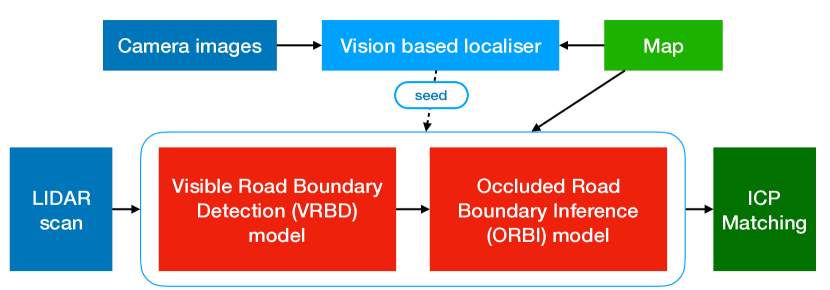
Figure 1: On overview of the pipeline proposed in this paper. After localisation is coarsely initialised, the live LiDAR scan is passed through our VRBD and ORBI models. This gives us not only visible road boundaries but also inferred locations for the occluded parts of those road boundaries. These are then matched to a map which has been similarly processed for visible and occluded road boundaries. Note that localisation is coarsely initialised by a camera stream but this part of the system is interchangeable with e.g. LiDAR place recognition systems such as [5].

II Related Work

Mapping and localisation techniques can be classified into two groups: global and relative [6].

Global techniques for localisation of a robot can be achieved using Global Navigation Satellite Systems (GNSS), but it is not precise enough for autonomous driving as the accuracy is worse than 2-3 metres in an open-sky environment [7]. Indeed, consider Figure 3. We observe that there are many gaps along the route when samples from the Oxford RobotCar Dataset [8] are overlaid on a digital map using Global Positioning System (GPS) coordinates. Relative techniques based on Simultaneous Localisation and Mapping (SLAM) [9] or ego-motion estimation [10] do not employ a global frame of reference but are less susceptible to drift and scale better with vast environments.

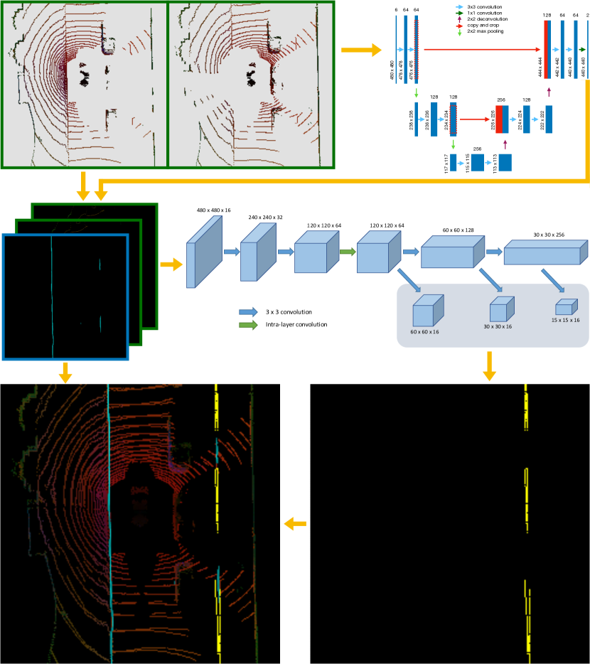
Figure 2: Our LIDAR-based coupled approach for road boundary detection. Given a pair of IPM images from left and right LIDARs, the fully convolutional VRBD model detects visible road boundaries and then passes to the ORBI model for inference of occluded road boundaries. The second model contains 3 base layers, intra-layer convolutions and 3 layers of parameterised multi-scale predictions at the end.

Depending on the type of input sensor these approaches can be further categorised by their use of cameras (passive sensors) and LiDARs or radars (active sensors). Camera-based techniques, such as Visual Odometry (VO) [11], are sensitive to lighting conditions, shadows, illumination, under- and overexposure [12]. Using dense maps in LiDAR-based approaches, such as Laser Odometry (LO) [13], is usually very accurate but computationally expensive for running in real-time. There is burgeoning interest in radar-based techniques, including Radar Odometry (RO) [14, 15, 16] and localisation [17]. As of yet, these techniques do not offer a rich enough understanding of scene semantics to be employed for road boundary problems.

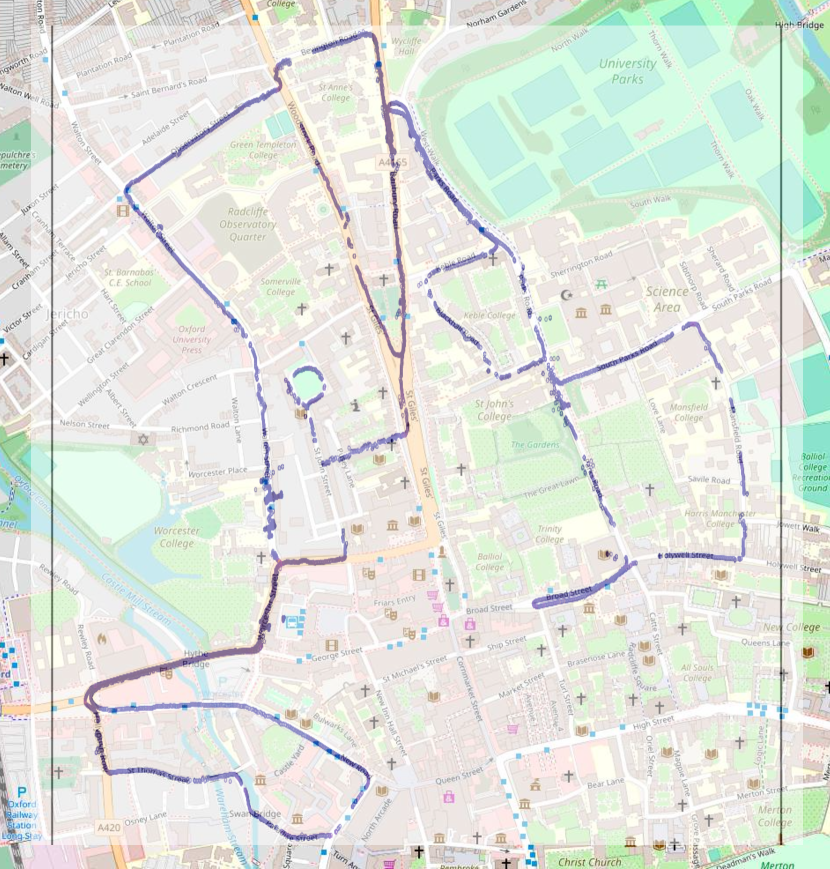
Figure 3: Samples of vehicle position are overlaid on a digital map using GPS coordinates. Although the dataset is a complete loop, we observe many gaps along the route.

Finally, regardless of the sensor used, feature matching is often used to match inputs from the sensors to maps. Indeed, Lane markings, traffic signs, feature points or road boundaries can be used as features for localisation [18]. The long and continuous shape of road boundaries makes them stable and robust features for localisation in the lateral direction as they capture the structure of roads.

In this paper we use sparse LiDAR-based detected road boundaries for computational ease and infer occluded road boundaries to meet the challenge of partially or fully occlusion by obstacles or other road users.

III Methodology

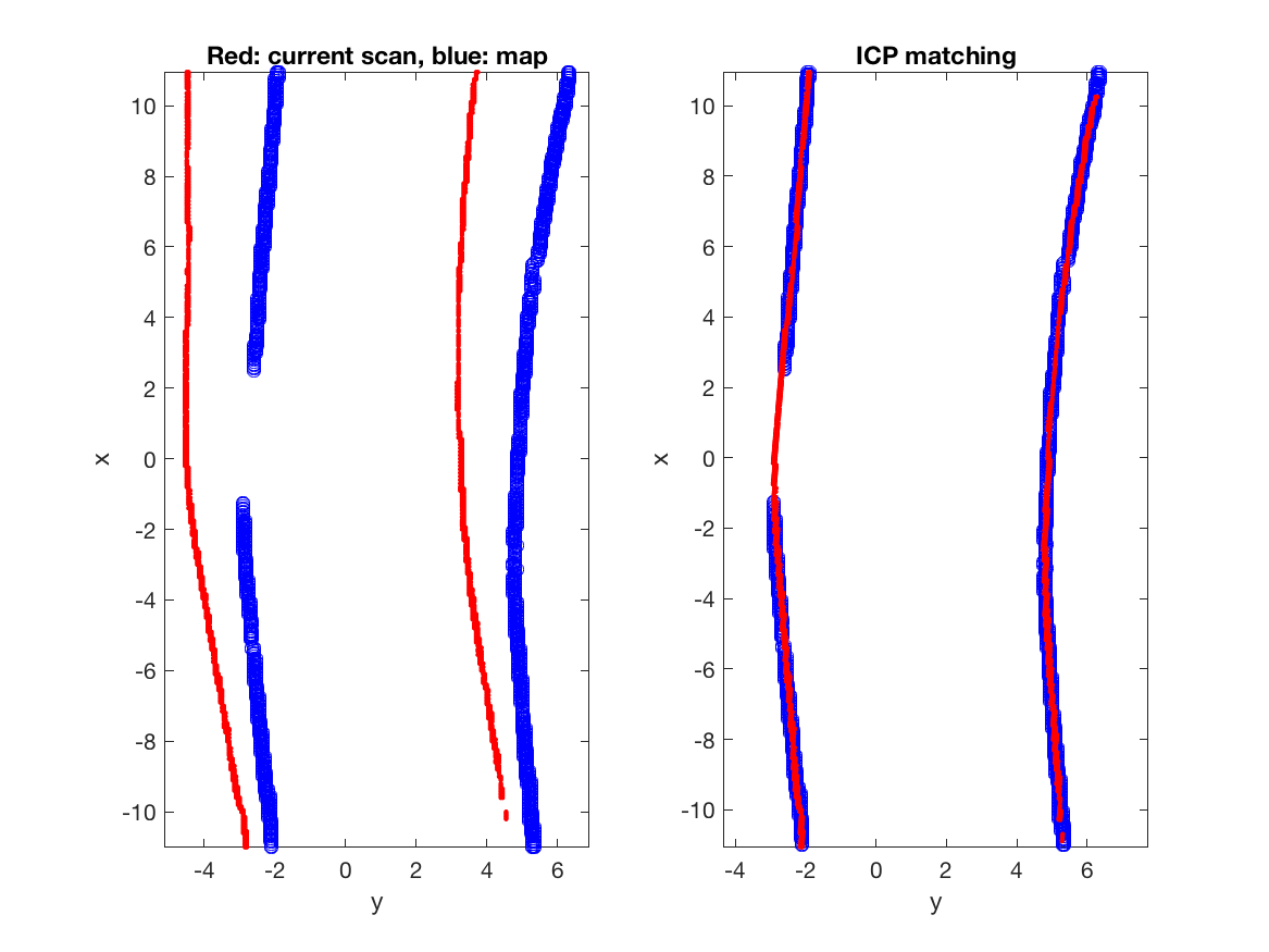
Figure 4: Given the detected road boundaries mask of a scan, it is binarised and transformed into a point cloud to match with a scan from the map. ICP is used to match the road boundaries and estimate the transformations between the frames. This example shows the accurate estimation of the transformation despite the undetected section of the road boundaries in the map frame.

Our cross-track localisation approach, the workflow for which is shown in Figure 1, is designed to:

1. Demonstrate usability of the outputs of a LiDAR-based road boundary detection approach for lateral localisation, and

2. Demonstrate a gain in performance that inferring of occluded road boundaries could bring.

This section details (in Sections III-B and III-C) the two subsystems inherent to our pipeline. As to be detailed in Section IV-A, the system acts between a map and a live trajectory, each taken from a different dataset (or collection of sensory records captured during a foray by the vehicle). We begin by describing a preprocessing step for all map and live LiDAR scans.

III-A LiDAR IPM

Labels and 3D LiDAR scans are transformed into 2D bird’s eye view images – or IPMs– to obtain input images and their road boundary masks. Note that the 3D LiDAR scans are trimmed to keep only the points that are close to the road surface before transforming them into IPM images. Our test vehicle has two 3D LiDARs and we generate IPM images for both of them before combining them in a single frame, accounting for the six degree-of-freedom (6DoF) extrinsic offset in sensor mount positions.

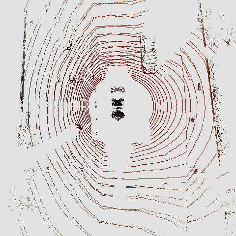
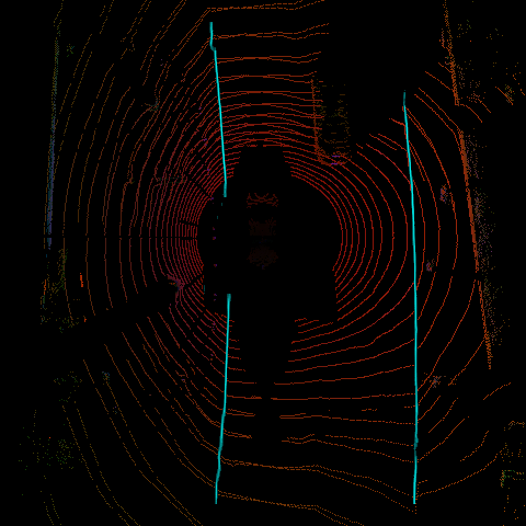
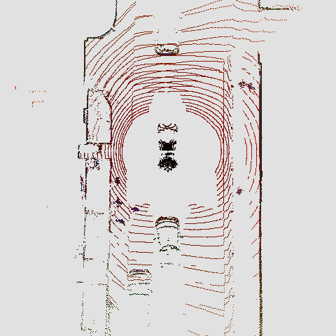
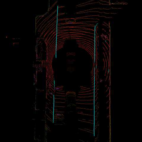
Figure 5: Output samples of detected visible road boundaries by the VRBD model with a ROI of 24x24 squared metre.

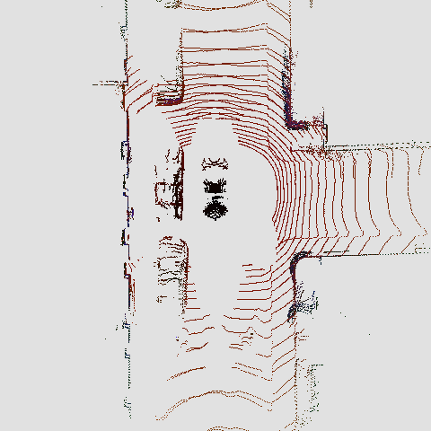
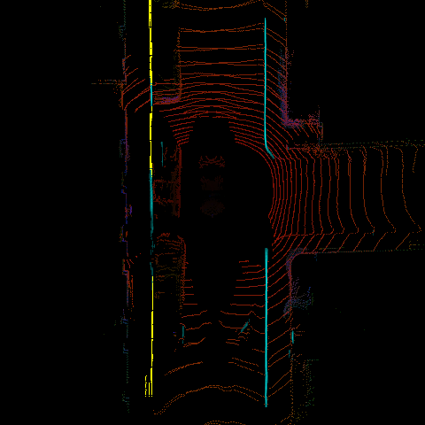
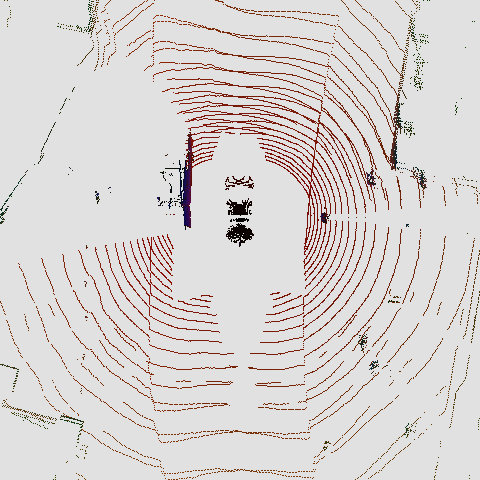
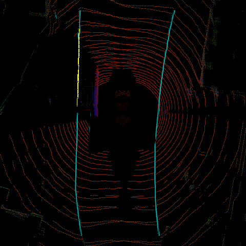
Figure 6: Output samples of detected visible and inferred occluded road boundaries by the VRBD and ORBI models with a ROI of 24x24 squared metre.

III-B Visible and occluded road boundary detection

We adopt our LiDAR-based VRBD and ORBI models presented in [2, 3] to run the inference over the map dataset with the region of interest (ROI) of 24x24 squared metre, where 1 px correspond to $5\text{\,}\mathrm{cm}$ in the real world. Outputs of the detected road boundaries are stored in the map with corresponding timestamps. Figure 2 shows and describes this in more detail. Figures 5 and 6 show examples of visible-only road boundary detection as well as inference of the position of occluded road boundaries.

III-C Map matching

The second dataset is used as a live input and the detected road boundaries from the second dataset are matched against the map dataset to perform lateral localisation. We assume that the initial guess of the location of the vehicle in the map are provided by a vision-based localiser [19]. Note that the vision-based localiser only provides timestamps of corresponding images from the map without providing initial pose. We use the ICP algorithm [20] to perform the matching process and estimate the transformations between the live inputs and the map. ICP is a well-known algorithm that is used for matching point clouds, where the algorithm iteratively updates the transformation between two point clouds to minimise the distance between them. We adopt ICP to estimate the transformation between live and map samples. The detected road boundary masks are binarised and converted into point clouds and then matched with ICP as shown in Figure 4.

IV Experimental Setup

This section details our experimental design in obtaining the results to follow in Section V.

IV-A Dataset curation

To run our experiments we use a pair of datasets – one dataset as a map and the other as a live input. Our experiments cover two pairs of datasets in central Oxford, one taken from [8] and the other from [21]. The pair taken from [8] are collected in April, 2018 and January 2019, respectively, and we refer to this experiment as Experiment 1. The pair taken from [21] are both collected in January, 2019 and we refer to this experiment as Experiment 2.

IV-B Data annotation

Fine-grained hand annotation of road boundaries from images would be a very time consuming process and it would be impossible to exactly annotate position of occluded road boundaries. To avoid that we annotate 3D point clouds that are collected using 2D laser. We then accumulate subsequent vertical laser scans in a coherent coordinate frame using VO to estimate vehicle’s motion in order to compute transformations between subsequent scans.

IV-C Performance metrics

Our results are relative measures of improved LiDAR lateral localisation when including detections of occluded road boundaries over systems which do not have access to those detections and only use visible road boundaries. We compare the agreement of the returned poses to the pose available from a state-of-the-art vision-based localiser [19].

V Results

This section presents instrumentation of the metrics discussed in Section IV over both experiments: Experiment 1 and Experiment 2.

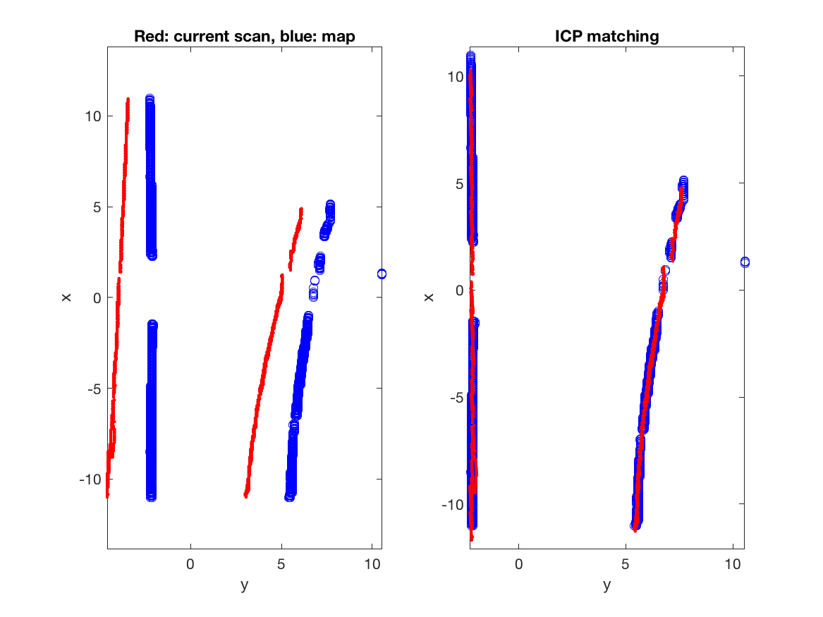
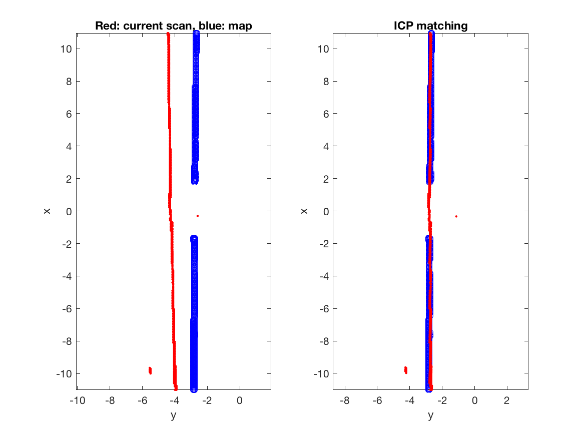
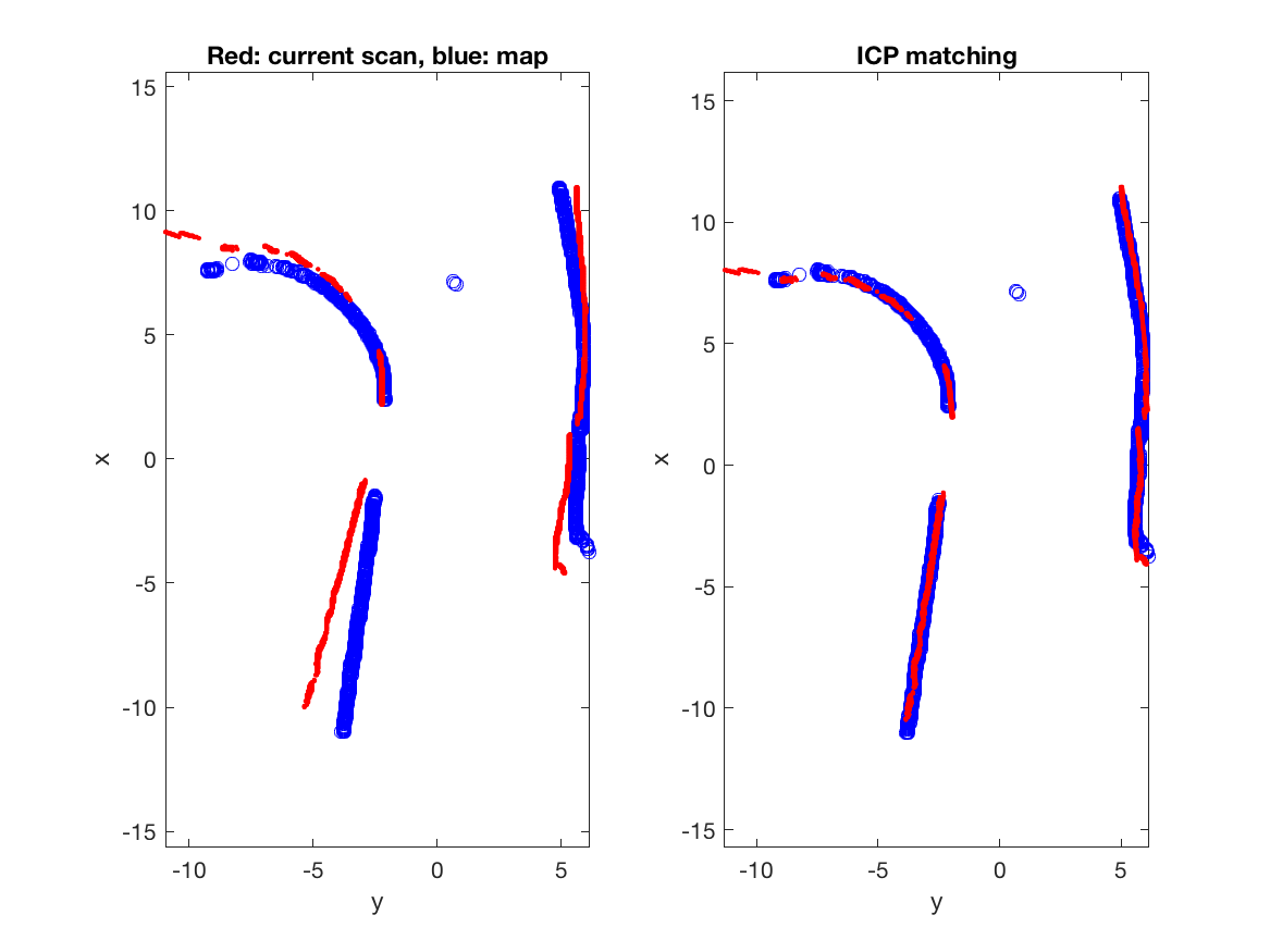
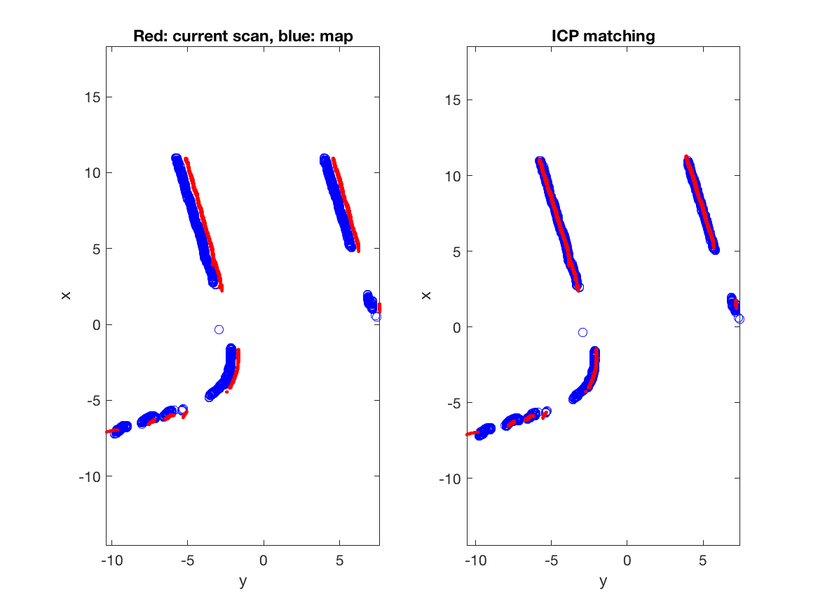
Figure 7: Examples of road boundary based ICP matching for localisation. These examples demonstrate that ICP accurately estimates the transformations between samples irrespective of the structure of the detected road boundaries since the detected road boundaries between samples are balanced over the sections of the true boundaries. Results obtained by processing the Experiment 1 dataset pair.

We present in Figure 7 qualitative examples of road boundary based ICP matching for localisation. These examples demonstrate that ICP accurately estimates the transformations between samples irrespective of the structure of the detected road boundaries. Small amounts of noise in the detection does not change the overall estimation of the transformations given that the road boundaries are detected in a balanced way over the sections of the true boundaries. ICP can accurately estimate the transformation in the presence of detected road boundaries on one side of the road.

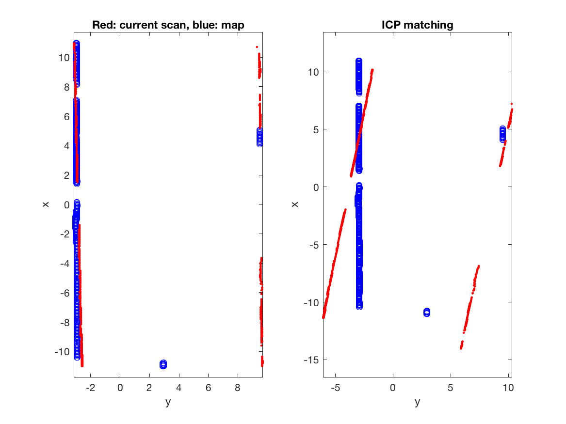
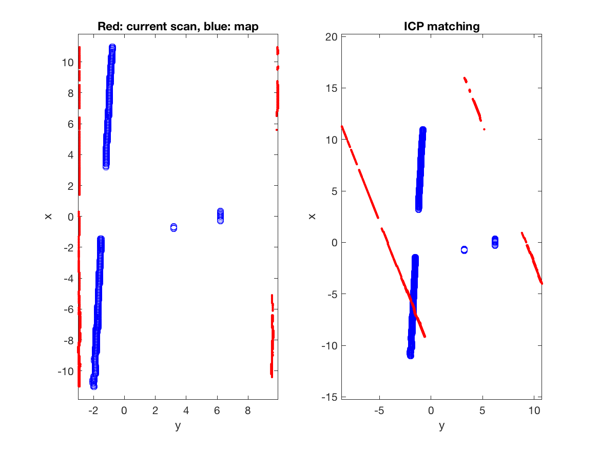
Figure 8: ICP matching failure examples, where the detected road boundaries on the right hand side of the road are unbalanced between samples. Results obtained by processing the Experiment 1 dataset pair.

Consider Figure 8. In these illustrated cases ICP fails to match the road boundaries accurately to generate transformations between samples. This happens when the detected road boundaries between live and map inputs are unbalanced, which forces ICP to rotate the live inputs as keeping them parallel is more costly. This can be fixed using more sophisticated matching techniques. Consider, however, Figure 9 in which we include in the matching detections of occluded road boundaries as proposed in this paper. Without more sophisticated matching techniques, we are now able to obtain sane transformations.

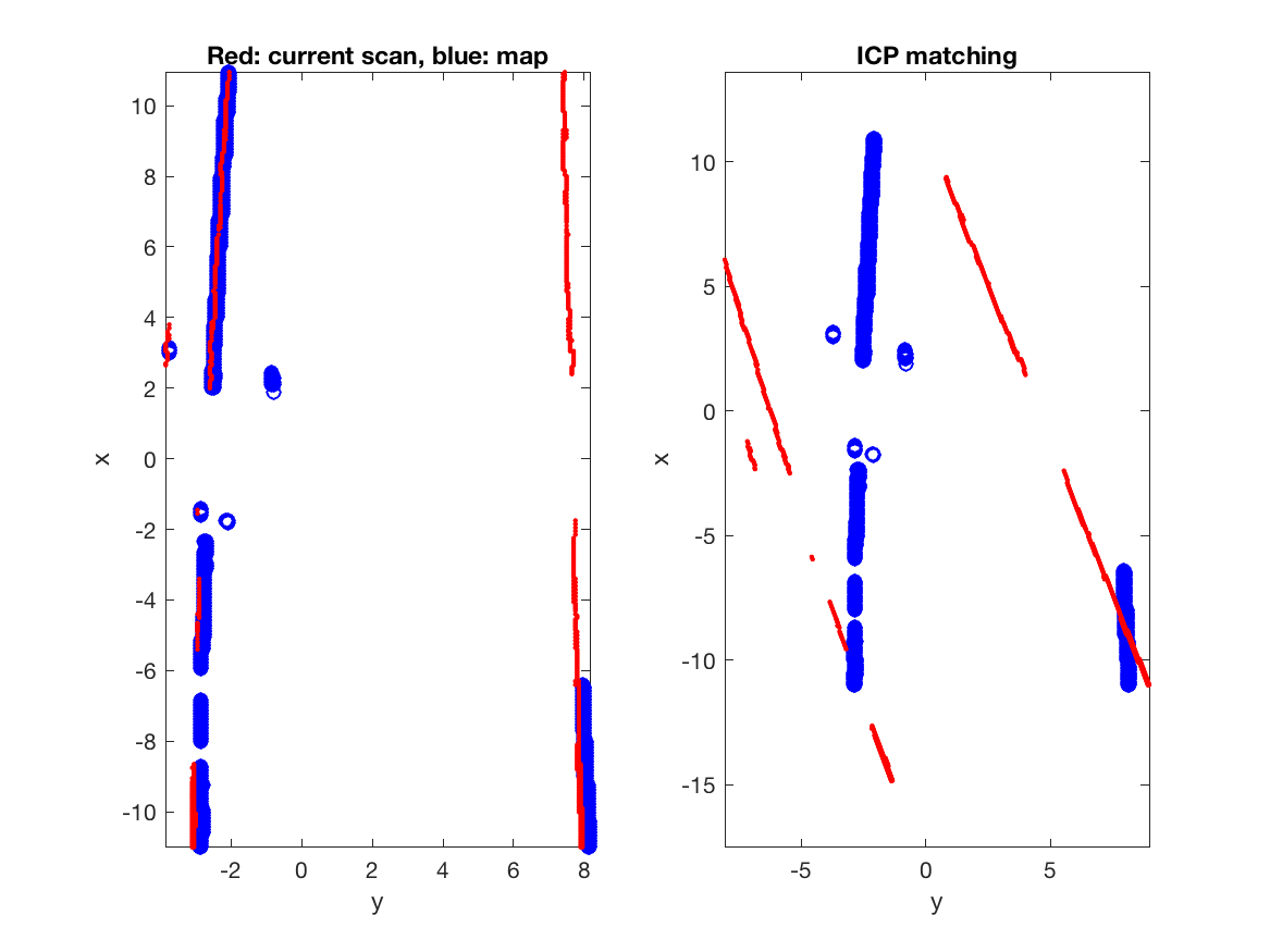
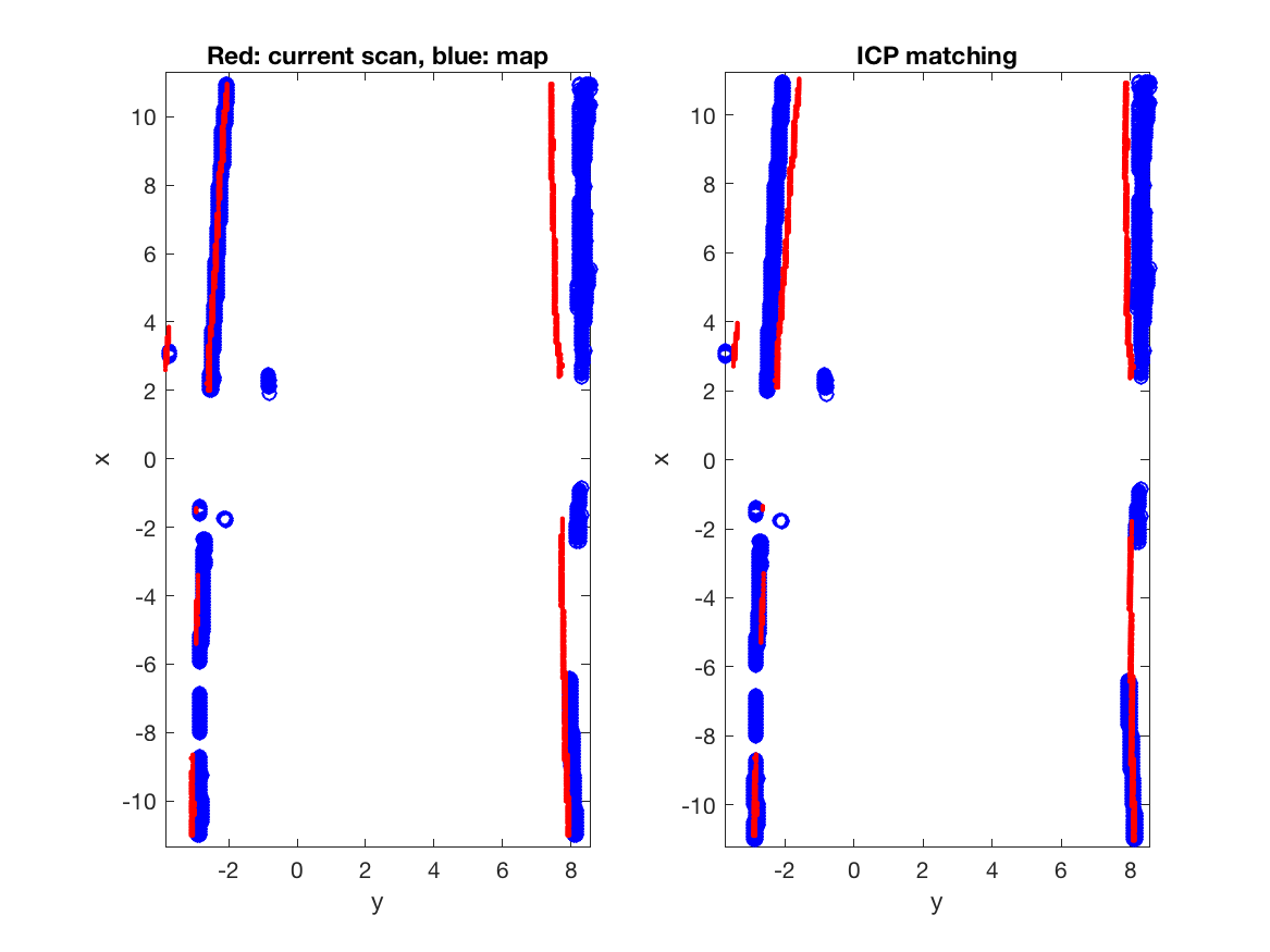
Figure 9: Comparison: ICP matching based on detected visible road boundaries only (top) and based on all road boundaries (bottom). Results obtained by processing the Experiment 1 dataset pair.

Table I: Road boundary based lateral localisation results, comparing localisation based on visible road boundaries only with localisation based on a combination of visible and occluded road boundaries. The results show that using the inferred occluded road boundaries always improves performance. Results obtained by processing the Experiment 1 dataset pair.

	Visible only		Visible and occluded
Error range	Number of samples	Percentage	Number of samples	Percentage
Within 0.1 metre	20389	65.56%	21934	70.53%
Within 0.3 metre	27479	88.36%	28349	91.15%
Within 0.5 metre	29005	93.26%	29617	95.23%
Within 1 metre	30124	96.86%	30504	98.08%

Table II: Average lateral localisation error for both the Experiment 1 and Experiment 2 dataset pairs.

Matching method	Map dataset	Live dataset	Visible only	Visible and occluded
ICP	2018-04-30	2019-01-18	18.95 cm	14.72 cm
ICP	2019-01-10-11	2019-01-10-12	18.54 cm	12.18 cm
ICP with worst rejection	2019-01-10-11	2019-01-10-12	9.33 cm	7.51 cm

We compare in Tables I, II, 10, 11, 12 and 13 the estimated road boundary based lateral localisation results with the lateral localisation of the vision-based localiser. Note that the IPM images that are used for estimating the lateral localisation are interpolated to match the timestamps of the camera images that the vision-based localiser uses.

Here, we calculate average lateral error (mean absolute error) and yaw error for the lateral localisation based on:

1. Visible road boundaries only, and

2. A combination of all road boundaries.

For Experiment 1, our results show that the average lateral localisation error based on visible road boundaries only is $18.95\text{\,}\mathrm{cm}$. Including the inferred occluded road boundaries decreases the error by $4.23\text{\,}\mathrm{cm}$ to $14.72\text{\,}\mathrm{cm}$. Similarly, the yaw error decreases from $0.0332\text{\,}\mathrm{rad}$ to $0.0206\text{\,}\mathrm{rad}$. Similar boons to performance for Experiment 2 can be read from Table II.

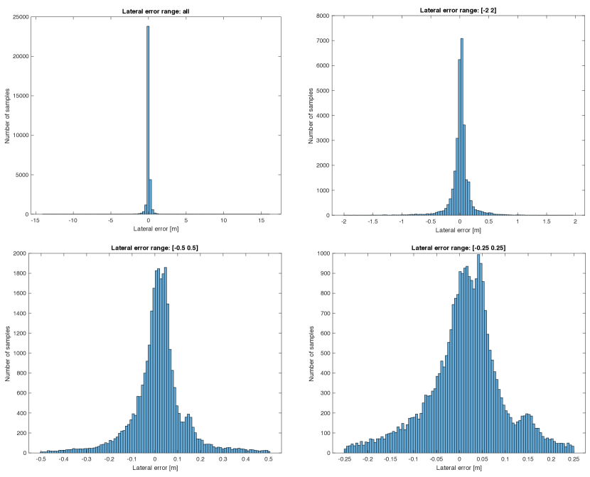
Figure 10: Histograms of road boundary based lateral error. The top left histogram includes all samples from the dataset, while the remaining histograms progressively narrow the displayed error range (horizontal axis). We observe that the majority of the samples (70.53%) have a maximum lateral error smaller than 10 cm. Results obtained by processing the Experiment 1 dataset pair.

We analyse in Figures 10 and I the output results by counting the number of samples that have a lateral error within 1, 0.5, 0.3, and 0.1 metres. Using the inferred occluded road boundaries increases the percentage of the number of samples within 1 metre from 96.86% to 98.08% Similar gains are achieved for the number of samples within 0.5, 0.3, and 0.1 metres. Overall, 70.53% of samples have lateral error less than 10 cm in contrast with the vision-based localiser. To visualise the lateral error of the samples we will plot them as histograms.

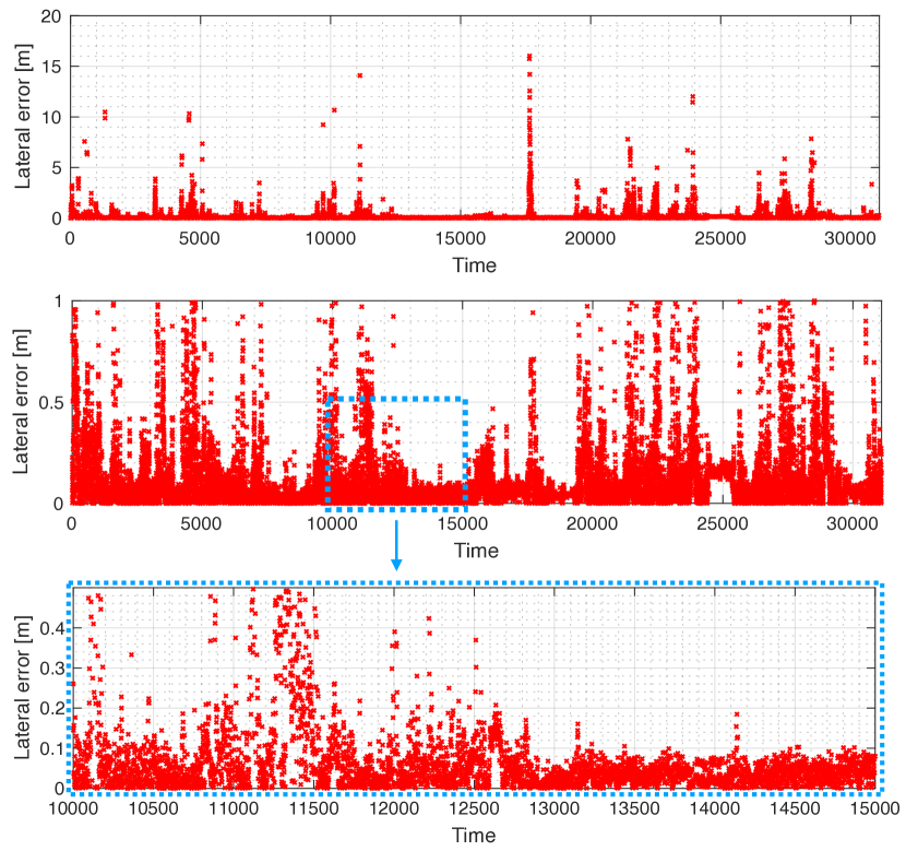
Figure 11: Lateral error of all samples displayed in a timeline (top), where we observe that there are only a small number of peaks where localisation failed. Progressively narrowing the displayed error range (vertical axis) shows that the majority of the samples (70.53%) have a maximum lateral error within 10 cm. Results obtained by processing the Experiment 1 dataset pair.

The lateral error of all samples are displayed in the timeline of Figure 11 to show that the majority of the samples (98.08%) has an error less than one metre and there are only a small number of peaks where localisation fails. We also plot a zoomed in section of the timeline to show that the large number of samples (70.53%) has a lateral error less than 10 cm.

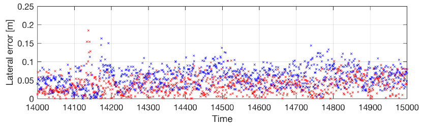
Figure 12: A timeline of 1000 samples, displaying lateral errors based on only visible road boundaries (blue points) and errors based on all road boundaries (red points). We observe that the blue points are generally larger than the red ones, indicating that using all road boundaries is better for performance. Results obtained by processing the Experiment 1 dataset pair.

Another timeline plotted in Figure 12 contains only 1000 samples and shows the importance of occluded road boundaries. The blue points in the figure represent the lateral error based on only visible road boundaries, where the red points are the localisation errors with all road boundaries. Overall, we observe that the blue points (only visible road boundaries) have higher values than the red ones (visible and occluded road boundaries).

Finally, Figure 13 shows distributions of the magnitude of localisation failure for Experiment 2. These can be understood as the probability that a localisation failure (measured as a lateral deviation) will occur on a given localisation run. We observe for all ranges of failures the inclusion of inferred positions of occluded road boundaries is beneficial to the robustness of a lateral localisation system.

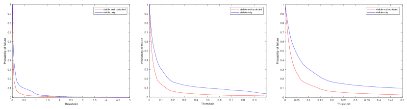
Figure 13: Probability that a localisation failure (measured as a lateral deviation in the $y$-direction) will occur on a given localisation run. Results obtained by processing the Experiment 2 dataset pair.

VI Conclusions

In this paper we presented a road boundary based lateral localisation method that provides accurate results using LiDAR data. The proposed system leverages new methods for detecting occluded road boundaries in sparse LiDAR data to improve LiDAR-based lateral localisation beyond that which is currently possible by naïve visible road boundary detection based methods. This is particularly evident and relevant in environments which are challenged by dense traffic conditions. Additionally, the proposed system is innovative in comparison to systems which may rely on GPS initialisation of the lateral localisation system by fusing the initial pose hint from onboard sensors such as cameras (although the method is agnostic to how this hint is sourced), which is particularly important in GPS-denied environments. This is also beneficial in comparison to existing systems which perform along-path localisation with LiDARs and rely in that sense on the detection of objects in the scene (e.g. traffic signs), which may also be occluded (or missing) in particularly challenging environments. We demonstrated that using inferred occluded road boundaries improves performance in environments which are challenged by the presence of obstructions.

VII Future Work

In the future we plan to integrate the system on the all-weather platform described in [22] in challenging, unstructured environments, requiring a new labelling regime to identify the boundaries of driveable paths.

References

- [1] T. Suleymanov, L. M. Paz, P. Piniés, G. Hester, and P. Newman, “The Path Less Taken: A Fast Variational Approach for Scene Segmentation Used for Closed Loop Control,” in IEEE/RSJ International Conference on Intelligent Robots and Systems (IROS), Daejeon, South Korea, Oct. 2016.
- [2] T. Suleymanov, P. Amayo, and P. Newman, “Inferring road boundaries through and despite traffic,” in The 21st IEEE International Conference on Intelligent Transportation Systems, Nov. 2018.
- [3] T. Suleymanov, L. Kunze, and P. Newman, “Online inference and detection of curbs in partially occluded scenes with sparse lidar,” in The 22nd IEEE International Conference on Intelligent Transportation Systems, Oct. 2019.
- [4] L. Kunze, T. Bruls, T. Suleymanov, and P. Newman, “Reading between the lanes: Road layout reconstruction from partially segmented scenes,” in IEEE International Conference on Intelligent Transportation Systems (ITSC), Maui, Hawaii, USA, Nov. 2018.
- [5] G. Kim, B. Park, and A. Kim, “1-day learning, 1-year localization: Long-term LiDAR localization using scan context image,” IEEE Robotics and Automation Letters, vol. 4, no. 2, pp. 1948–1955, 2019.
- [6] S. Thrun, D. Fox, W. Burgard, and F. Dellaer, “Robust monte carlo localization for mobile robots,” Artificial Intelligence, vol. 101, p. 99–141, 2001.
- [7] F. Ghallabi, F. Nashashibi, G. El-Haj-Shhade, and M.-A. Mittet, “Lidar-based lane marking detection for vehicle positioning in an hd map,” in IEEE 21th International Conference on Intelligent Transportation Systems (ITSC), Maui, Hawaii„ United States, Nov. 2018.
- [8] W. Maddern, G. Pascoe, C. Linegar, and P. Newman, “1 Year, 1000km: The Oxford RobotCar Dataset,” The International Journal of Robotics Research (IJRR), vol. 36, no. 1, pp. 3–15, 2017.
- [9] G. Grisetti, R. Kummerle, C. Stachniss, and W. Burgard, “A tutorial on graph-based slam,” IEEE Intelligent Transportation Systems Magazine, vol. 2, no. 4, pp. 31–43, 2010.
- [10] J. Borenstein and L. Feng, “Measurement and correction of systematic odometry errors in mobile robots,” IEEE Transactions on robotics and automation, vol. 12, no. 6, pp. 869–880, 1996.
- [11] D. Nistér, O. Naroditsky, and J. Bergen, “Visual odometry,” in Proceedings of the 2004 IEEE Computer Society Conference on Computer Vision and Pattern Recognition, 2004. CVPR 2004., vol. 1. Ieee, 2004, pp. I–I.
- [12] C. McManus, W. Churchill, W. Maddern, A. D. Stewart, and P. Newman, “Shady dealings: Robust, long-term visual localisation using illumination invariance,” in 2014 IEEE international conference on robotics and automation (ICRA). IEEE, 2014, pp. 901–906.
- [13] J. Zhang and S. Singh, “Loam: Lidar odometry and mapping in real-time.” in Robotics: Science and Systems, vol. 2, no. 9, 2014.
- [14] S. H. Cen and P. Newman, “Precise ego-motion estimation with millimeter-wave radar under diverse and challenging conditions,” in 2018 IEEE International Conference on Robotics and Automation (ICRA). IEEE, 2018, pp. 1–8.
- [15] R. Aldera, D. De Martini, M. Gadd, and P. Newman, “What Could Go Wrong? Introspective Radar Odometry in Challenging Environments,” in IEEE Intelligent Transportation Systems Conference (ITSC), Auckland, New Zealand, October 2019.
- [16] R. Aldera, D. De Martini, M. Gadd, and P. Newman, “Fast Radar Motion Estimation with a Learnt Focus of Attention using Weak Supervision,” in IEEE International Conference on Robotics and Automation (ICRA), May 2019, pp. 1190–1196.
- [17] \cbS. Săftescu, M. Gadd, D. De Martini, D. Barnes, and P. Newman, “Kidnapped Radar: Topological Radar Localisation using Rotationally-Invariant Metric Learning,” arXiv preprint arXiv: 2001.09438, 2020. [Online]. Available: https://arxiv.org/abs/2001.09438
- [18] P. Sun, X. Zhao, Z. Xu, R. Wang, and H. Min, “A 3D LiDAR Data-Based Dedicated Road Boundary Detection Algorithm for Autonomous Vehicles,” IEEE Access, vol. 7, pp. 29 623–29 638, 2019.
- [19] C. Linegar, W. Churchill, and P. Newman, “Work Smart, Not Hard: Recalling Relevant Experiences for Vast-Scale but Time-Constrained Localisation,” in Proceedings of the IEEE International Conference on Robotics and Automation (ICRA), Seattle, WA, USA, May 2015.
- [20] P. J. Besl and N. D. McKay, “A method for registration of 3-d shapes,” IEEE Transactions on Pattern Analysis and Machine Intelligence, vol. 14, no. 2, pp. 239–256, Feb. 1992.
- [21] D. Barnes, M. Gadd, P. Murcutt, P. Newman, and I. Posner, “The Oxford Radar RobotCar Dataset: A Radar Extension to the Oxford RobotCar Dataset,” arXiv preprint arXiv: 1909.01300, 2019. [Online]. Available: https://arxiv.org/pdf/1909.01300
- [22] S. Kyberd, J. Attias, P. Get, P. Murcutt, C. Prahacs, M. Towlson, S. Venn, A. Vasconcelos, M. Gadd, D. De Martini, and P. Newman, “The Hulk: Design and Development of a Weather-proof Vehicle for Long-term Autonomy in Outdoor Environments,” in International Conference on Field and Service Robotics (FSR), Tokyo, Japan, August 2019.