Mixed fluid cosmological model in $f(R,T)$ gravity

Abstract

We construct Locally Rotationally Symmetric (LRS) Bianchi type-I cosmological model in $f(R,T)$ theory of gravity when the source of gravitation is the mixture of barotropic fluid and dark energy (DE) by employing a time varying deceleration parameter (DP). We observe through the behavior of the state finder parameters $(r,s)$ that our model begins from the Einstein static era and goes to $\Lambda$CDM era. The EoS parameter($\omega_{d}$) for DE varies from phantom ($\omega<-1$) phase to quintessence ($\omega>-1$) phase which is consistent with the observational results. It is found that the discussed model can reproduce the current accelerating phase of expansion of the universe.

I Introduction

The latest cosmological observation detects the expansion of the universe as an accelerating rate Riess/1998 ; Perlmutter/1999 . This has led us to consider the exotic matter, dark energy, as a clarification and proof of this late time acceleration. DE existence has been supported by various observational data which includes – Cosmic Microwave Background (CMB) anisotropy Bernardis/2000 ; Bennett/2003 ; Hanany/2000 , Large Scale Structure (LSS) Spergel/2003 ; Tegmark/2004 ; MTegmark/2004 , Sloan Digital Sky Survey (SDSS)Tegmark/2004 ; MTegmark/2004 ; Seljak/2005 ; Adelman/2006 , Wilkinson Microwave Anisotropy Probe Knop/2003 (WMAP) and Chandra X-ray observatory Allen/2004 . A further investigation has established our universe composition as $73\%$ dark energy, $23\%$ dark matter and only $4\%$ as baryonic matter. DE is a scalar field of negative pressure with positive energy which serves as a means for reverse gravitational action Riess/2004 ; Tonry/2003 . This explains the shift from early time inflation to late time acceleration.

DE can be explained in two ways. The first one is by choosing any of the exotic matter options viz. – quintessence Martin/2008 ; Wetterich/1988 ; Ratra/1988 , phantom Nojiri/2006 , $k$- essence Chiba/2000 ; Armendariz/1999 ; Armendariz/2000 , tachyons Padmanabhan/2002 , quintom Nojiri/2004 , chaplygin gas Srivastava/2005 ; Bertolami/2004 ; Bento/2002 ; Bilic/2002 ; Avelino/2003 ; Kamenshchik/2001 , chameleon Khoury/2004 , cosmological nuclear energy Gupta/2010 and cosmological constant Overduin/1998 ; Sahni/2000 ; Komatsu/2009 ; Kachru/2003 . Out of these, the approach of cosmological constant is the simplest and most general to explain the acceleration but it incorporates the problems related to cosmic coincidence and fine-tuning Sahni/2000 ; Weinberg/1989 ; Peebles/2003 . However, these choices are insufficient to explain the mystery of dark energy completely. DE model is outlined using the Equation of State (EoS) parameter $\omega$ which defined as in terms of pressure and energy density such that; $\omega(t)=\frac{p}{\rho}$. This parameter need not be a constant Carroll/2003 . It can be parametrized as in terms of time or scale factor ($a$) or redshift ($z$).

The second way to explain DE is by modifying the theory of gravity. These theories serve natural gravitational alternatives to DE and attempt to justify current acceleration. Various modified theories are $f(R),f(G),f(T)$ and $f(R,T)$. The generalization of the Lagrangian in Einstein-Hilbert action where, function $f(R)$ is used instead of $R$, Ricci scalar gives $f(R)$ theory of gravity SNojiri/2011 . This theory serves as a consolidation of early time inflation with late time acceleration. The model handles higher order curvature invariants as a function of $R$. A further generalization of $f(R)$ gravity theory yields $f(R,T)$ theory which was originally introduced by Harko et al. Harko/2011 . The authors considered Lagrangian density as a function $f(R,T)$, where $T$ denotes the trace of energy momentum tensor. This model, contrast to other theories, discuss matter and geometry coupling. This results in source term independence, where source term is the matter stress energy tensor variant. They claim that cosmic acceleration is also a result of matter content besides geometrical input. Thereafter, many researchers are interested to do more investigations of this theory through various aspects Houndjo/2012 ; Jamil/012 ; Alvarenga/2013 ; Houndjo/2014 ; Sahoo/017 ; PKSahoo/2017 ; Sharif/12 ; Alvarenga/013 . In Shabani/2013 FLRW cosmological model has been studied in the framework of $f(R,T)$ gravity through phase space analysis. We can see in refs.Sahoo/2016 ; Sahoo/2017 ; Sahoo/0017 it has been studied for different matter components. Recently, V. Fayaz et al. Fayaz/2017 studied Bianchi-I space-time in this theory where they regenerated $f(R,T)$ function using holographic dark energy. They reproved that the rate of evolution of the anisotropic universe is greater than that of FRW and $\Lambda$CDM model.

Yadav et al. Yadav/2011 discussed the DE model in Bianchi type-III universe with constant DP ($q$). The EoS parameter $\omega$ is established as a time dependent factor in the respective case. Naidu et al. examined spatially homogeneous and anisotropic Bianchi type II Reddy/2012 and III RLNaidu/2012 models based on Saez and Ballester theory. Based on the same theory, the authors also investigated Bianchi type V Naidu/2012 model with variable $\omega$ and constant $q$. Kotambkar et al. GPSingh/2014 constructed anisotropic Bianchi type I model with bulk viscosity and quintessence and discussed various physical properties of the model. Singh et al. Singh/2014 examined Bianchi type II model for a perfect fluid source in $f(R,T)$ gravity. The solutions were obtained using the power law relation between mean Hubble parameter ($H(t)$) and average scale factor ($a(t)$). The same conditions were worked upon by Reddy et al. Reddy/2013 using the special law of variation for Hubble’s parameter given by Berman Berman/1983 . The special law generates constant DP which implies exclusion of open universes. Samanta sam13 constructed a model of the universe filled with dark energy from a wet dark fluid in $f(R,T)$ gravity. Samanta and Dhal samanta13 studied Bianchi type- V universe with a binary mixture of perfect fluid and dark energy in $f(R,T)$ gravity. Sahoo and Mishra sah14 investigated Kaluza-Klein dark energy model in the form of wet dark fluid in $f(R,T)$ gravity. Singh and Sharma Singh/2014 constructed Bianchi type-II dark energy cosmological model with variable EoS parameter in $f(R,T)$ gravity. By considering constant DP they obtained two models of the universe, namely, power law model and exponential model. Yadav et al yad15 obtained dark energy dominated universe in $f(R,T)$ gravity with hybrid law expansion. Rao et al. Rao/2015 applied the same law to investigate 5-dimensional Kaluza-Klein space time in the existence of anisotropic dark energy in $f(R,T)$ gravity. Bishi bis16 studied Bianchi type-III dark energy model in $f(R,T)$ gravity with variable DP. Chaubey et al. cha16 considered general class of Bianchi cosmological models in $f(R,T)$ gravity with the dark energy in the form of standard and modified Chaplygin gas. Sahoo sah17 considered Kaluza-Klein universe filled with wet dark fluid in $f(R,T)$ gravity and obtained the exact solutions from a time varying DP.

In this work, we use both the approach concurrently. That is we considered the source of gravitational matter as a mixture of perfect fluid and dark fluid in a modified theory called $f(R,T)$ theory. This type of simultaneous use of both the approach have already been used by the authors baf17 and sha17 .

The work being organized in the following manner: In Section-I, Introduction and motivations from the literature are briefly elaborated. Section-II contains the basic formalism of $f(R,T)$ gravity general field equations. The solution of the field equation for LRS Bianchi type-I metric by employing time varying DP are presented in Section-III. At last the Physical behavior of the model and conclusions are outlined in Section-IV and Section-V respectively.

II The $f(R,T)=R+2f(T)$ gravity

Field equation for $f(R,T)$ gravity can be formulated from the Hilbert-Einstein in the following manner.

$$S=\frac{1}{16\pi G}\int\sqrt{-g}f(R,T)d^{4}x+\int\sqrt{-g}L_{m}d^{4}x,$$ (1)

where $L_{m}$ is the matter Lagrangian density, $g$ is the determinant of the metric tensor $g_{ij}$, $R$ is Ricci scalar and $T$ is the trace of energy-momentum tensor $T_{ij}$. The energy-momentum tensor $T_{ij}$ is defined as

$$T_{ij}=-\frac{2}{\sqrt{-g}}\frac{\delta(\sqrt{-g}L_{m})}{\delta g^{ij}}.$$ (2)

Here, Instead of considering the derivative of matter Lagrangian, we have assumed that the matter Lagrangian $L_{m}$ depends only on the metric components. Such as

$$T_{ij}=g_{ij}L_{m}-\frac{\partial L_{m}}{\partial g^{ij}}.$$ (3)

The $f(R,T)$ gravity field equations are obtained from the eqn. (1) by varying the action $S$ with respect to metric component. It is given as

$$f_{R}(R,T)R_{ij}-\frac{1}{2}f(R,T)g_{ij}+(g_{ij}\Box-\nabla_{i}\nabla_{j})f_{R}(R,T)=8\pi T_{ij}-f_{T}(R,T)T_{ij}-f_{T}(R,T)\Theta_{ij},$$ (4)

where

$$\Theta_{ij}=-2T_{ij}+g_{ij}L_{m}-2g^{lm}\frac{\partial^{2}L_{m}}{\partial g^{ij}\partial g^{lm}},$$ (5)

and $f_{R}(R,T)=\frac{\partial f(R,T)}{\partial R}$, $f_{T}(R,T)=\frac{\partial f(R,T)}{\partial T}$, $\Box\equiv\nabla^{i}\nabla_{i}$, where $\nabla_{i}$ is the covariant derivative.

To construct different kind of cosmological models according to the choice of matter source, Harko et al. Harko/2011 constructed three types of $f(R,T)$ gravity as follows

$$f(R,T)=\left\{\begin{array}[]{lcl}R+2f(T)&&\\ f_{1}(R)+f_{2}(T)&&\\ f_{1}(R)+f_{2}(R)f_{3}(T)&&\end{array}\right.$$ (6)

The general field equation for first frame of $f(R,T)=R+2f(T)$ gravity is given as

$$R_{ij}-\frac{1}{2}Rg_{ij}=8\pi T_{ij}-2f^{\prime}(T)T_{ij}-2f^{\prime}(T)\Theta_{ij}+f(T)g_{ij}.$$ (7)

III Field equations and Solutions

We consider the spatially homogeneous LRS Bianchi type-I metric as

$$ds^{2}=dt^{2}-A^{2}(dx^{2}+dy^{2})-B^{2}dz^{2},$$ (8)

where $A$, $B$ are functions of cosmic time $t$ only.
The stress-energy momentum tensor is in the form

$$T_{j}^{i}=T_{(m)j}^{i}+T_{(de)j}^{i},$$ (9)

where $T_{(m)j}^{i}$ and $T_{(de)j}^{i}$ are energy momentum tensor of perfect fluid and dark energy respectively. These are given by

$$T_{(m)j}^{i}=diag[\rho_{m},-p_{m},-p_{m},-p_{m}],$$ (10)

and

$$T_{(de)j}^{i}=diag[\rho_{d},-p_{d},-p_{d},-p_{d}],$$ (11)

where $p_{m}$, $\rho_{(m)}$ are pressure and energy density for perfect fluid and $p_{d}$, $\rho_{d}$ are pressure and the energy density for dark energy components respectively.

The field eqn. (7) with $f(T)=\alpha T$, where $\alpha$ is an arbitrary constant, becomes

$$R_{ij}-\frac{1}{2}Rg_{ij}=(8\pi+2\alpha)T_{ij}+(2\alpha p+\alpha T)g_{ij}.$$ (12)

In the framework of $f(R,T)$ gravity, in the term $(2\alpha p+\alpha T)$, $p$ is the isotropic pressure and $T$ is the trace of energy-momentum tensor. According to poplawski06 and poplawski006 the trace of energy momentum tensor is of isotropic pressure and energy density i.e. $T=\rho-3p$.
The field eqn. (12) for the line element (8) is given as

$$-\dot{H_{1}}-H_{1}^{2}-\dot{H_{2}}-H_{2}^{2}-H_{1}H_{2}=(8\pi+2\alpha)(p_{m}+p_{d})-\alpha(\rho_{m}-p_{m}),$$ (13)

$$-2\dot{H_{1}}-3H_{1}^{2}=(8\pi+2\alpha)(p_{m}+p_{d})-\alpha(\rho_{m}-p_{m}),$$ (14)

$$2H_{1}H_{2}+H_{1}^{2}=(8\pi+2\alpha)(\rho_{m}+\rho_{d})+\alpha(\rho_{m}-p_{m}).$$ (15)

Here $H_{1}=\frac{\dot{A}}{A}$, $H_{2}=\frac{\dot{B}}{B}$ and the over dot represent derivatives with respect to cosmic time $t.$ We have six unknowns $H_{1}$, $H_{2}$, $\rho_{m}$, $\rho_{d}$, $p_{m}$, & $p_{d}$ and three equations. In order to obtain the exact solution, we have assumed in first step the Bianchi identity $G^{ij}_{;j}=0$ as it is followed from the definition of the Einstein tensor $G_{ij}$ and $R_{ij}$ Misner/1970 . From which we have obtained the following relation.

$$\dot{\rho_{m}}+3(1+\omega_{m})\rho_{m}H=0,$$ (16)

where $H=\frac{\dot{a}}{a}=\frac{1}{3}(\frac{2\dot{A}}{A}+\frac{\dot{B}}{B})$ is mean Hubble parameter, $a=(A^{2}B)^{\frac{1}{3}}$ is the average scale factor and $\omega_{m}=\frac{p_{m}}{\rho_{m}}$ is EoS parameter of perfect fluid considered as a constant akarsu10 . From eqn. (16) we obtain the value of $\rho_{m}$ as

$$\rho_{m}=c_{1}a^{-3(1+\omega_{m})},$$ (17)

where $c_{1}$ is an integration constant. Following Chawla13 we have considered the time varying DP of the form

$$q=-\frac{a\ddot{a}}{\dot{a}^{2}}=b(t),$$ (18)

This geometric parameter has vital role in the description of the evolution of the universe, which defines the phase transition of the universe from past decelerating expansion to the recent accelerating one. Thus, it is well motivated to consider a time-dependent DP $q$ is due to the fact that the universe exhibits phase transitions, as revealed by the cosmic observations of SNe Ia. Also, the transitional phase of the universe can be determined by the signature flipping nature of DP, i.e. positive DP defines decelerating phase and negative sign of DP represents the accelerating phase of late universe. Thus, the choice of time-dependent DP is physically reliable for cosmological models. The expression of $q$ given in eqn. (18) can be written as

$$\frac{\ddot{a}}{a}+b\frac{\dot{a}^{2}}{a^{2}}=0.$$ (19)

By assuming $b=b(a)$ or $b=b(a(t))$, the general solution of (19) is given as

$$\int e^{\int\frac{b}{a}}da=t+\textit{d},$$ (20)

where d is a constant of integration. In order to derive the solution (20), without any loss of generality, one can choose $\int\frac{b}{a}da=\ln f(a)$, and eqn. (20) yields

$$\int f(a)da=t+\textit{d}.$$ (21)

In this eqn. (21), the arbitrary function $f(a)$ can be chosen in such a way that, it will provide a physically viable and observationally consistent cosmological model. Thus, $f(a)$ is considered as

$$f(a)=\frac{na^{n-1}}{\beta\sqrt{(}1+a^{2n})},$$ (22)

where $\beta$ is an arbitrary constant and $n$ is a positive constant. Using eqn. (22) in eqn. (21) and taking $\textit{d}=0$, we obtain the following exact solution is

$$a(t)=[\sinh(\beta t)]^{\frac{1}{n}}.$$ (23)

Then the directional scale factors $A$ and $B$ are derived from the relation $V=a^{3}$ as follows

$$A(t)=[\sinh(\beta t)]^{\frac{1}{2n}},$$ (24)

$$B(t)=[\sinh(\beta t)]^{\frac{2}{n}}.$$ (25)

Now the line element (8) can be rewritten as

$$ds^{2}=dt^{2}-[\sinh(\beta t)]^{\frac{1}{n}}(dx^{2}+dy^{2})-[\sinh(\beta t)]^{\frac{4}{n}}dz^{2}.$$ (26)

From equations (14) and (15), the values of $p_{d}$, $\rho_{d}$ and $\omega_{d}$ are obtained as

$$\rho_{d}=\frac{c_{1}(\alpha(\omega_{m}-3)-8\pi)\left(\left(\frac{1}{z+1}\right)^{n}\right)^{-\frac{3(\omega_{m}+1)}{n}}+\frac{9\beta^{2}\left(\left(\frac{1}{z+1}\right)^{-2n}+1\right)}{4n^{2}}}{2(\alpha+4\pi)},$$ (27)

$$p_{d}=\frac{c_{1}(-3\alpha\omega_{m}+\alpha-8\pi\omega_{m})\left(\left(\frac{1}{z+1}\right)^{n}\right)^{-\frac{3(\omega_{m}+1)}{n}}-\frac{\beta^{2}\left(\frac{1}{z+1}\right)^{-2n}\left(3\left(\frac{1}{z+1}\right)^{2n}-4n+3\right)}{4n^{2}}}{2(\alpha+4\pi)},$$ (28)

$$\omega_{d}=-\frac{4c_{1}n^{2}(\alpha(3\omega_{m}-1)+8\pi\omega_{m})\left(\frac{1}{z+1}\right)^{2n}+\beta^{2}\left(3\left(\frac{1}{z+1}\right)^{2n}-4n+3\right)\left(\left(\frac{1}{z+1}\right)^{n}\right)^{\frac{3(\omega_{m}+1)}{n}}}{9\beta^{2}\left(\left(\frac{1}{z+1}\right)^{2n}+1\right)\left(\left(\frac{1}{z+1}\right)^{n}\right)^{\frac{3(\omega_{m}+1)}{n}}-4c_{1}n^{2}(8\pi-\alpha(\omega_{m}-3))\left(\frac{1}{z+1}\right)^{2n}}.$$ (29)

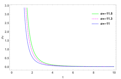
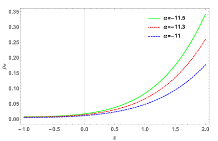
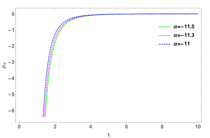
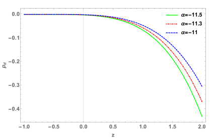
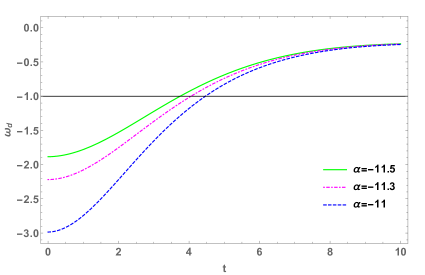
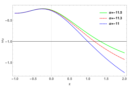
The variation of energy density, pressure and equation of state (EoS) parameter with cosmic time t are shown in the following figures. In Fig. 2, the energy density $\rho_{d}$ is a positive decreasing function of time and tends to zero at $t$ tends to $\infty$. Fig. 4 represents the graphics for pressure $p$, which is a negative increasing function of time and tends to zero at $t$ tends to $\infty$. As per the observation, the negative pressure is due to DE in the context of accelerated expansion of the universe. Hence, the behavior of pressure in our model agrees with this observation. In Fig. 6, the EoS parameter lies in the accelerated phase dominated by DE era. From Fig. 6, one can observe that the EoS parameter shows a transitional behavior. In Figs. 2, 4, and 6, the variation of energy density, pressure and equation of state (EoS) parameter with redshift parameter $z$ are depicted respectively, and it provides the reliability of the model.

Figure 1: Variation of $\rho$ against time with $\beta=0.09804$, $n=1.15$, $c_{1}=0.001$, $\omega_{m}=0.5$.

Figure 2: Variation of $\rho$ against $z$ with $\beta=0.09804$, $n=1.15$, $c_{1}=0.001$, $\omega_{m}=0.5$.

Figure 3: Variation of $p$ against time with $\beta=0.09804$, $n=1.15$, $c_{1}=0.001$, $\omega_{m}=0.5$.

Figure 4: Variation of $p$ against $z$ with $\beta=0.09804$, $n=1.15$, $c_{1}=0.001$, $\omega_{m}=0.5$.

Figure 5: Variation of Eos Parameter against time with $\beta=0.09804$, $n=1.15$, $c_{1}=0.001$, $\omega_{m}=0.5$.

Figure 6: Variation of Eos Parameter against $z$ with $\beta=0.09804$, $n=1.15$, $c_{1}=0.001$, $\omega_{m}=0.5$.

IV Physical properties of the models

The values of various physical parameters viz. DP, energy density of perfect fluid ($\rho_{m}$), mean Hubble parameter ($H$), expansion scalar ($\theta$), shear scalar ($\sigma^{2}$) and mean anisotropic parameter ($A_{m}$) for the model are obtained as

$$q=n\text{sech}^{2}(\beta t)-1=\frac{n}{\left(\frac{1}{z+1}\right)^{2n}+1}-1,$$ (30)

$$\rho_{m}=c_{1}\sqrt[n]{\sinh(\beta t)}^{-3\omega-3}=c_{1}\left(\beta\left(\frac{1}{z+1}\right)^{n}\right)^{\frac{-3\omega_{m}-3}{n}},$$ (31)

$$H=\frac{\beta\coth(\beta t)}{n}=\frac{\beta\left(\frac{1}{z+1}\right)^{-n}\sqrt{\left(\frac{1}{z+1}\right)^{2n}+1}}{n},$$ (32)

$$\theta=3H=\frac{3\beta\coth(\beta t)}{n}=\frac{3\beta\left(\frac{1}{z+1}\right)^{-n}\sqrt{\left(\frac{1}{z+1}\right)^{2n}+1}}{n},$$ (33)

$$\sigma^{2}=\frac{3\beta^{2}\coth^{2}(\beta t)}{4n^{2}}=\frac{3\beta^{2}\left(\frac{1}{z+1}\right)^{-2n}\left(\left(\frac{1}{z+1}\right)^{2n}+1\right)}{4n^{2}},$$ (34)

$$A_{m}=\frac{3}{2}.$$ (35)

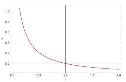
One of the important quantities for the dynamical description of the universe is known as state finder pair or $r-s$ parameter. It helps to study the coincidence between obtained model with $\Lambda$CDM model. For flat $\Lambda$CDM model, the value of state finder pair yields as $\{r,s\}=\{1,0\}$ Feng/2008 . The values of the $r-s$ parameter of our model becomes

$$r=\frac{\dot{\ddot{a}}}{aH^{3}}=n(2n-3)\text{sech}^{2}(\beta t)+1=\frac{n(2n-3)}{\left(\frac{1}{z+1}\right)^{2n}+1}+1,$$ (36)

$$s=\frac{r-1}{3(q-\frac{1}{2})}=\frac{n(2n-3)\text{sech}^{2}(\beta t)}{3\left(n\text{sech}^{2}(\beta t)-1.5\right)}=\frac{2(3-2n)n}{\left(\frac{1}{z+1}\right)^{2n}-6n+1}.$$ (37)

Figure 7: Evolution of r-s parameter with $\beta=0.09804$, $n=1.15$.

The matter energy density $(\Omega_{m})$ and dark energy density ($\Omega_{d}$) are obtained as

$$\Omega_{m}=\frac{c_{1}n^{2}\left(\frac{1}{z+1}\right)^{2n}\left[\left(\left(\frac{1}{z+1}\right)^{n}\right)^{1/n}\right]^{-3\omega_{m}-3}}{3\beta^{2}\left(\left(\frac{1}{z+1}\right)^{2n}+1\right)},$$ (38)

and

$$\Omega_{d}=\frac{\left(\left(\frac{1}{z+1}\right)^{n}\right)^{-\frac{3(\omega_{m}+1)}{n}}\left[9\beta^{2}\left(\left(\frac{1}{z+1}\right)^{2n}+1\right)\left(\left(\frac{1}{z+1}\right)^{n}\right)^{\frac{3(\omega_{m}+1)}{n}}-4c_{1}n^{2}(8\pi-\alpha(\omega_{m}-3))\left(\frac{1}{z+1}\right)^{2n}\right]}{24(\alpha+4\pi)\beta^{2}\left(\left(\frac{1}{z+1}\right)^{2n}+1\right)}.$$ (39)

Adding eqns. (38) and (39) we get the total energy $(\Omega)$ as

$$\Omega=\frac{n^{2}\left(\frac{1}{z+1}\right)^{2n}\left[\frac{c_{1}(\alpha(\omega_{m}-3)-8\pi)\left(\left(\frac{1}{z+1}\right)^{n}\right)^{-\frac{3(\omega_{m}+1)}{n}}+\frac{9\beta^{2}\left(\left(\frac{1}{z+1}\right)^{-2n}+1\right)}{4n^{2}}}{2(\alpha+4\pi)}+c_{1}\left(\left(\frac{1}{z+1}\right)^{n}\right)^{-3/n}\left[\left(\left(\frac{1}{z+1}\right)^{n}\right)^{1/n}\right]^{-3\omega_{m}}\right]}{3\beta^{2}\left(\left(\frac{1}{z+1}\right)^{2n}+1\right)}.$$ (40)

From eqn. (30) we find that $q<0$, hence the model represents an accelerating universe. Since $\displaystyle{\lim_{t\to\infty}}\frac{\sigma^{2}}{\theta^{2}}\neq 0$ the universe is anisotropic throughout the evolution. Fig. 7 shows the variation of $s$ with respect to $r$. It is clear from this figure that $s$ is negative when $r$ is greater than one. As $r\rightarrow\infty$, $s\rightarrow-\infty$ and when $r=1$ we have $s=0$. Hence the universe starts from the Einstein static era and goes to $\Lambda$CDM era.

V Conclusion

The LRS Bianchi type-I cosmological model in $f(R,T)$ gravity theory is constructed in this paper with the exact solutions of the field equations. In $f(R,T)$ gravity, cosmic acceleration depends on geometric contribution as well on matter content of the universe. Cosmological models with a source of dark energy yield a very good approximation to the accelerated expansion of the universe. As a result, in this obtained model we can see the behavior of the energy density and pressure with respect to time in Fig. 2 and Fig. 4 and with respect to redshift parameter $z$ in Fig. 2 and Fig. 4. From Fig. 2 one can observe that at initial epoch the energy density of the universe is very high. As time increases it decreases and approaches to zero when $t\rightarrow\infty$. Energy density remains positive throughout the evolution of the universe. From Fig. 4 we see that the universe starts with a very large negative pressure, decreases with increase in cosmic time $t$ and approaches to zero for large $t$. This reveals the characteristic behavior of the dark energy. The nature of EoS parameter ($\omega_{d}$) for DE with the evolution of cosmic time $t$ is shown in Fig. 6 and with respect to redshift parameter $z$ is shown in Fig. 6. The parameter $\omega>-1$ and $\omega<-1$ correspond quintessence and phantom energy respectively attributes present accelerated expansion of the universe. Also, The evolution of energy density, pressure and EoS parameter correspond to redshift parameter $z$ are depicted in details in the Figs. 2, 4, and 6 respectively. It can be observed that the universe is dominated by dark energy which may be the strongest evidence for present cosmic expansion. All of the solutions obtained are consistent with the observational results. Hence we feel that these results will be helpful for the researchers to realize the characteristics of the universe in the framework of $f(R,T)$ theory.

VI Acknowledgements

The authors would like to thank Prof. P. K. Sahoo for discussion and valuable suggestions. We are grateful to DST, New Delhi, India for providing facilities through DST-FIST lab, Department of Mathematics, where a part of this work was done. The authors also thank the anonymous referee for the comments and suggestions that helped us to improve the manuscript.

References

- (1) A. G. Riess et al., Observational Evidence from Supernovae for an Accelerating Universe and a Cosmological Constant, The Astronomical Journal, 116 (1998) 1009-1038.
- (2) S. Perlmutter et al., Measurements of and from 42 High-Redshift Supernovae, The Astrophysical Journal, 517 (1999) 565-586.
- (3) P. de Bernardis et al., A flat universe from high-resolution maps of the cosmic microwave background radiation, Nature,404( 2000) 955-959 .
- (4) C. L. Bennett et al., First year Wilkinson microwave anisotropy probe (WMAP) observations: Preliminary maps and basic results, The Astrophysical Journal Supplement Series, 148 (2003) 1–27.
- (5) S. Hanany et al., MAXIMA-1: A measurement of the cosmic microwave background anisotropy on angular scales of , The Astrophysical Journal Letters, 545 (2000) L5-L9.
- (6) D. N. Spergel et al., First-year Wilkinson microwave anisotropy probe (WMAP) observations: Determination of cosmological parameters, The Astrophysical Journal Supplement Series, 148, (2003)175-194.
- (7) M. Tegmark et al., The 3D power spectrum of galaxies from the SDSS, The Astrophysical Journal, 606 (2004) 702-740.
- (8) M. Tegmark et al., Cosmological parameters from SDSS and WMAP, Physical Review D, 69 (2004) 103501.
- (9) U. Seljak et al., Cosmological parameter analysis including SDSS Ly forest and galaxy bias: Constraints on the primordial spectrum of fluctuations, neutrino mass and dark energy, Physical Review D, 71 (2005) 103515.
- (10) J. K. Adelman-McCarthy et al., The fourth data release of the Sloan Digital Sky Survey-SDSS collaboration, The Astrophysical Journal Supplement Series, 162 (2006) 38–48.
- (11) R. A. Knop et al., New constraints on , and from an independent set of eleven high-redshift supernovae observed with the Hubble Space Telescope, The Astrophysical Journal, 598 (2003) 102-137.
- (12) S. W. Allen, et al., Constraints on dark energy from Chandra observations of the largest relaxed galaxy clusters, Monthly Notices of the Royal Astronomical Society, 353 (2004) 457–467.
- (13) A. G. Riess et al., Type Ia supernova discoveries at from the Hubble Space Telescope: Evidence for past deceleration and constraints on dark energy evolution, The Astrophysical Journal, 607(2004) 665–687.
- (14) J. L. Tonry et al., Cosmological results from high-z supernovae, The Astrophysical Journal, 594(2003) 1–24 .
- (15) J. Martin, Quintessence: A mini-review, Modern Physics Letters A, 23 (2008) 1252-1265.
- (16) C. Wetterich, Cosmology and the fate of dilatation symmetry, Nuclear Physics B, 302 (1988) 668-696.
- (17) B. Ratra, P. J. E. Peebles, Cosmological consequences of a rolling homogeneous scalar field, Physical Review D, 37 (1988) 3406-3427.
- (18) S. Nojiri, S. D. Odintsov, The oscillating dark energy: future singularity and coincidence problem, Physics Letters B,637 (2006) 139-148.
- (19) T. Chiba, T. Okabe, M. Yamaguchi, Kinetically driven quintessence, Physical Review D 62 (2000) 023511.
- (20) C. Armendariz-Picon, T. Damour, V. Mukhanov, -Inflation, Physics Letters B, 458 (1999) 209-218.
- (21) C. Armendariz-Picon, V. Mukhanov, P. J. Steinhardt, A Dynamical Solution to the Problem of a Small Cosmological Constant and Late-time Cosmic Acceleration, Physical Review Letters, 5 (2000) 4438-4441.
- (22) T. Padmanabhan, T. R. Choudhury, Can the clustered dark matter and the smooth dark energy arise from the same scalar field?, Physical Review D, 66 (2002) 081301.
- (23) S. Nojiri, S. D. Odintsov, The minimal curvature of the universe in modified gravity and conformal anomaly resolution of the instabilities, Modern Physics Letters A,19 (2004) 627-638.
- (24) S. K. Srivastava, Future Universe With Without Big Smash, Physics Letters B, 619 (2005) 1-4.
- (25) O. Bertolami, A. A. Sen, S. Sen, P. T. Silva, Latest supernova data in the framework of the generalized Chaplygin gas model, Monthly Notices of the Royal Astronomical Society, 353 (2004) 329-337.
- (26) M. C. Bento, O. Bertolami, A. A. Sen, Generalized Chaplygin gas, accelerated expansion, and dark-energy-matter unification, Physical Review D, 66 (2002) 043507.
- (27) N. Bilic, G. B. Tupper, R. D. Viollier, Unification of Dark Matter and Dark Energy: the Inhomogeneous Chaplygin Gas, Physics Letters B,535 (2002)17-21.
- (28) P. P. Avelino, et al., Alternatives to quintessence model building, Physical Review D, 67 (2003) 023511.
- (29) A. Kamenshchik, U. Moschella, V. Pasquier, An alternative to quintessence, Physics Letters B, 511, (2001) 265-268.
- (30) J. Khoury, A. Weltman, Chameleon Fields: Awaiting Surprises for Tests of Gravity in Space, Physical Review Letters, 93 (2004) 171104.
- (31) R. C. Gupta, A. Pradhan, Genesis of Dark Energy: Dark Energy as Consequence of Release and Two-Stage Tracking of Cosmological Nuclear Energy, International Journal of Theoretical Physics, 49, (2010) 821-834.
- (32) J. M. Overduin, F. I. Cooperstock, Evolution of the scale factor with a variable cosmological term, Physical Review D, 58, (1998) 043506.
- (33) V. Sahni, A. Starobinsky, The case for a positive cosmological -term, International Journal of Modern Physics D,9, (2000) 373-443.
- (34) E. Komatsu et al., Five-Year Wilkinson Microwave Anisotropy Probe Observations: Cosmological Interpretation, The Astrophysical Journal Supplement Series, 180 (2009) 330-376.
- (35) S. Kachru, et al., de Sitter vacua in string theory, Physical Review D, 68 (2003) 046005.
- (36) S. Weinberg, The cosmological constant problem, Reviews of Modern Physics, 61 (1989) 1-23.
- (37) P. J. E. Peebles, B. Ratra, The cosmological constant and dark energy, Reviews of Modern Physics, 75 (2003) 559-606.
- (38) S. M. Carroll, M. Hoffman, M. Trodden, Can the dark energy equation-of-state parameter be less than -1?, Physical Review D, 68 (2003) 023509.
- (39) S. Nojiri, S. D. Odintsov, Unified cosmic history in modified gravity: From theory to Lorentz non-invariant models, Physics Reports,505 (2011) 59-144.
- (40) T. Harko, F. S. N. Lobo, S. Nojiri, S. D. Odintsov, gravity, Physical Review D, 84 (2011) 024020.
- (41) M. J. S. Houndjo, Reconstruction of gravity describing matter dominated and accelerated phases, International Journal of Modern Physics D 21 (2012) 1250003.
- (42) M. Jamil, et al., Reconstruction of some cosmological models in gravity, Eurpian Physics Journal C 72 (2012) 1999.
- (43) F. G. Alvarenga, et al., Testing some gravity models from energy conditions, Journal of Modern Physics 04 (2013) 130-139.
- (44) M. J. S. Houndjo, Thermodynamics in little rip cosmology in the framework of a type of gravity, Europian Physics Journal Plus 129 (2014) 171.
- (45) P. K. Sahoo, Parbati Sahoo, Binaya K. Bishi, Sezgin Aygün ,Magnetized strange quark model with Big Rip singularity in gravity, Modern Physics Letter A 32 (2017) 1750105.
- (46) P. K. Sahoo, P. H. R. S. Moraes, Parbati Sahoo , Wormholes in -gravity within the f(R,T) formalism, Europian Physics Journal C 78 (2018) 46.
- (47) M. Sharif, M. Zubair, Thermodynamics in theory of gravity, Journal of Cosmological Astroparticle Physics 03 (2012) 028.
- (48) F. G. Alvarenga, et al., Dynamics of scalar perturbations in gravity, Physical Review D 87 (2013) 103526.
- (49) Hamid Shabani, Mehrdad Farhoudi, Cosmological Models in Phase Space, Physical Review D 88 (2013) 044048.
- (50) P.K. Sahoo, B. Mishra, Parbati Sahoo, S. K. J. Pacif, Bianchi type string cosmological models in gravity, Europian Physics Journal Plus, 131, (2016)333.
- (51) P.K. Sahoo, Parbati Sahoo, Binaya K. Bishi, Anisotropic cosmological models in gravity with variable deceleration parameter ,International Journal of Geometric Methods in Modern Physics, 14 (2017)1750097.
- (52) P. K. Sahoo, Parbati Sahoo, Binaya K. Bishi, Sezgin Aygün, Magnetized strange quark matter in gravity with bilinear and special form of time varying deceleration parameter, New Astronomy, 60 (2018) 80-87.
- (53) V. Fayaz, H. Hossienkhani, Z. Zarei, M. Ganji, N. Azimi, Anisotropic universe and reconstructing theory from holographic Ricci dark energy, Canadian Journal of Physics, 95 (2017) 524-534.
- (54) A. K. Yadav, L. Yadav, Bianchi Type III Anisotropic Dark Energy Models with Constant Deceleration Parameter, International Journal of Theoretical Physics, 50 (2011) 218-227.
- (55) R. L. Naidu, B. Satyanarayana, D. R. K. Reddy, LRS Bianchi type-II Universe with cosmic strings and bulk viscosity in a scalar tensor theory of gravitation, Astrophysics and Space Science, 338 (2012) 351-354.
- (56) R. L. Naidu, B. Satyanarayana, D. R. K. Reddy, Bianchi Type-III Dark Energy Model in a Saez-Ballester Scalar-Tensor Theory, International Journal of Theoretical Physics, 51 (2012) 2857-2862.
- (57) R. L. Naidu, B. Satyanarayana, D. R. K. Reddy, Bianchi Type-V Dark Energy Model in a Scalar-Tensor Theory of Gravitation, International Journal of Theoretical Physics, 51 (2012) 1997-2002.
- (58) S. Kotambkar, G. P. Singh, R. Kelkar, Anisotropic Cosmological Models with Quintessence, International Journal of Theoretical Physics, 53, (2014)449-460.
- (59) J. K. Singh, N. K. Sharma, Bianchi Type-II Dark Energy Model in Gravity, International Journal of Theoretical Physics, 53 (2014) 1424-1433.
- (60) D. R. K. Reddy, R. S. Kumar, T. V. P. Kumar, Bianchi type-III Dark Energy Model in Gravity, International Journal of Theoretical Physics, 52 (2013) 239-245.
- (61) M. S. Berman, A special law of variation for Hubble’s parameter, Nuovo Cimento B, 74 (1983) 182-186.
- (62) G. C. Samanta, Universe Filled with Dark Energy (DE) from a Wet Dark Fluid (WDF) in f(R,T) Gravity, Int. J. Theor. Phys., 52 (2013) 2303-2315.
- (63) G. C. Samanta, S. N. Dhala, Universe Filled with a Binary Mixture of Perfect Fluid and Dark Energy, Int. J. Theor. Phys., 52 (2013) 3092-3105.
- (64) P. K. Sahoo, B. Mishra, Kaluza-Klein dark energy model in the form of wet dark fluid in f(R,T) gravity, Can. J. Phys., 92 (2014) 1062-1067
- (65) A. K. Yadav, P. K. Srivastava, L. Yadav, Hybrid Expansion Law for Dark Energy Dominated Universe in f (R,T) Gravity, Int. J. Theor. Phys., 54 (2015) 1671-1679
- (66) V. U. M. Rao, D. C. P. Rao, Five dimensional anisotropic dark energy model in gravity, Astrophysics and Space Science, 357 (2015) 65.
- (67) B. K. Bishi, Variable deceleration parameter and dark energy models, Int. J. Geom. Methods Mod. Phys. 13 (2016) 1650055
- (68) R. Chaubey, A. K. Shukla, R. Raushan, T. Singh, The general class of Bianchi cosmological models in f (R, T) gravity with dark energy in viscous cosmology, Indian J. Phys. 90 (2016) 233-242
- (69) P. K. Sahoo, Kaluza-Klein Universe Filled with Wet Dark Fluid in f(R,T) Theory of Gravity, Acta Physica Polonica B Proceedings Supplement, 10 (2017) 369
- (70) E. H. Baffou, M. J. S. Houndjo, I. G. Salako, Viscous generalized Chaplygin gas interacting with f(R, T) gravity, Int. J. Geom. Methods Mod. Phys., 14 (2017) 1750051
- (71) H. Shabani, Cosmological consequences and statefinder diagnosis of a noninteracting generalized Chaplygin gas in f(R, T) gravity, Int. J. Mod. Phys. D, 26 (2017) 1750120
- (72) N. J. Poplawski, A Lagrangian description of interacting dark energy,(2006) arXiv:gr-gc/0608031.
- (73) N. J. Poplawski, Acceleration of the universe in the Einstein frame of a metric-affine gravity, Classical and Quantum Gravity 23 (2006) 2011-2020.
- (74) C. Misner, Thorne, K. S., and J. Wheeler, Gravitation (W.H. Freeman and Company, 1970).
- (75) O. Akarsu, C. B. Kilinc, LRS Bianchi type I models with anisotropic dark energy and constant deceleration parameter, General Relativity and Gravitation 42, 119 (2010).
- (76) C. Chawla, R. K. Mishra, A. Pradhan, Anisotropic Bianchi-I Cosmological Model in String Cosmology with Variable Deceleration Parameter. Romanian Journal of Physics, 58(2013) 1000-1013.
- (77) C.J. Feng, Statefinder Diagnosis for Ricci Dark Energy, Physics Letters B 670 (2008) 231.