Computer Aided Control System Design for Time Delay Systems using MATLAB^®

Abstract

Computer Aided Control System Design (CACSD) allows to analyze complex interconnected systems and design controllers achieving challenging control requirements. We extend CACSD to systems with time delays and illustrate the functionality of Control System Toolbox in MATLAB for such systems. We easily define systems in time and frequency domain system representations and build the overall complex system by interconnecting subsystems. We analyze the overall system in time and frequency domains and design PID controllers satisfying design requirements. Various visualization tools are used for analysis and design verification. Our goal is to introduce these functionalities to researchers and engineers and to discuss the open directions in computer algorithms for control system design.

1 Introduction

Time delays are frequently seen in many control applications such as process control, communication networks, automotive and aerospace, Dugard1998 ; NiculescuBook ; ErneuxBook . Depending on the delay length, they may limit or degrade the performance of control systems unless they are considered in the design, GuBook ; ComplexTDSBook . Although considerable research effort is devoted to extend classical and modern control techniques to accommodate delays, most available software packages for delay differential equations (DDE) retard ; enright ; BIFTOOLManual20 ; BredaTraceDDE09 are restrictive and not developed for control design purposes.

We present the currently implemented framework and available functionality in MATLAB for computer-aided manipulation of linear time-invariant (LTI) models with delays. We illustrate this functionality for each important step in every practical control design:

• system representations in time and frequency domains,

• interconnections of complex systems,

• analysis tools and design techniques for time delay systems.

By introducing available functionality in Control System Toolbox, our goal is to facilitate the design of control systems with delays for researchers and engineers. Moreover, we discuss possible enhancements in CASCD for time delay systems, to illustrate the gap between the desired analysis / design techniques and the current control software implementation.

At the heart of this framework is a linear fractional transformation (LFT) based representation of time delay systems lft . This representation handles delays in feedback loops and is general enough for most control applications. In addition most classical software tools for analyzing delay-free LTI systems are extended to this class of LTI systems with delays. Given the widespread use of linear techniques in control system design, this framework and the accompanying software tools should facilitate CACSD in the presence of delays, as well as stimulate more research into efficient numerical algorithms for assessing the properties and performance of such systems.

2 Motivation Examples

A standard PI control example is given in tankexample where the plant is a chemical tank and a single-input-single-output system with an input-output delay (i.e., dead-time system),

$$P(s)=e^{-93.9s}{5.6\over 40.2s+1}.$$ (1)

In the classical feedback configuration in Figure 1, the standard PI controller is chosen as

$$C_{PI}(s)=K(1+{1\over T_{i}s})$$ (2)

where $K=0.1$ and $T_{i}=100$. The closed-loop transfer function from $y_{sp}$ to $y$ is

$$T_{PI}(s)=\frac{4020s^{2}+100s}{4020s^{2}+100s+(56s+0.56)e^{-93.9s}}.$$

This transfer function has an internal delay which can not be represented by input or output delays. Therefore, the representation for time delay systems has to capture this type of systems and to be closed under block diagram of operations.

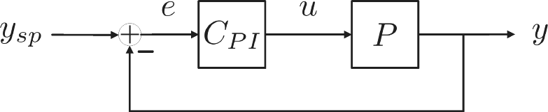
Figure 1: Feedback loop with PI controller.

This plant and the controller in MATLAB are defined as

  P = tf(5.6,[40.2 1],’OutputDelay’,93.9);   % plant
  Cpi = 0.1 * (1 + tf(1,[100 0]));           % PI controller

and the closed-loop system $T_{PI}$ is obtained by the feedback command:

  Tpi = feedback(P*Cpi,1);      % Closed-loop transfer, ysp -> y

Note that these commands are natural extensions of delay-free case and are used for systems with delays without new syntax for the user.

The MIMO time delay systems may have different transport delays for each input-output channel, i.e.,

$$H(s)=\left(\begin{array}[]{cc}e^{-0.1s}\frac{2}{s}&e^{-0.3s}\frac{s+1}{s+10}\\ 10&e^{-0.2s}\frac{s-1}{s+5}\\ \end{array}\right).$$

We define such systems in MATLAB by the following commands:

s = tf(’s’);
H = [2/s (s+1)/(s+10); 10 (s-1)/(s+5)];   % delay-free system
H.ioDelay = [0.1 0.3; 0 0.2];             % transport delays

We see on our motivation examples that the representation of time delay systems has certain challenges. Next section, we present the LFT-based representation of time delay systems to address these challenges and discuss its advantages.

3 System Representation

We represent time delay systems by the linear-fractional transformation (LFT). Recall that the LFT is defined for matrices by

$${\cal L}(\left(\begin{array}[]{cc}M_{11}&M_{12}\\ M_{21}&M_{22}\end{array}\right),\Theta):=M_{11}+M_{12}\Theta(I-M_{22}\Theta)^{-1}M_{21}\;.$$

The LFT has been extensively used in robust control theory for representing models with uncertainty, see lft for details.

Consider the class generalized LTI (GLTI) of continuous-time LTI systems whose transfer function is of the form

$$H(s,\tau)={\cal L}(\underbrace{\left(\begin{array}[]{cc}H_{11}(s)&H_{12}(s)\\ H_{21}(s)&H_{22}(s)\end{array}\right)}_{H(s)},\Theta(s,\tau))$$ (5)

$$\hskip 14.22636pt\Theta(s,\tau):={\rm Diag}\left(e^{-\tau_{1}s},\ldots,e^{-\tau_{N}s}\right)$$ (6)

where $H(s)$ is a rational (delay free) MIMO transfer function, and $\tau=(\tau_{1},\ldots,\tau_{N})$ is a vector of nonnegative time delays. Systems in this class are modeled as the LFT interconnection of a delay-free LTI model and a bank of pure delays (see Figure 2). As such, they are clearly linear time-invariant. Also, pure delays are in this class since $e^{-\tau s}={\cal L}(\left(\begin{array}[]{cc}0&1\\ 1&0\end{array}\right),e^{-\tau s})$.

Figure 2: LFT-based modeling of LTI systems with delays.

This GLTI class has two key properties, tdslft :

• Any block diagram interconnection of GLTI systems is a GLTI system. In other words, the class of GLTI systems is closed under series, parallel, and feedback connections as well as branching/summing junctions.

• The linearization of any nonlinear block diagram with time delays is a GLTI system.

These two properties show that the GLTI class is general enough to model any (linearized) system with a finite number of delays, including delays in the feedback path. For further motivation of this representation and equivalent case of discrete time systems, see tdslft .

The GLTI class is represented in state-space equations as follows. Let

$$\left(\begin{array}[]{cc}H_{11}(s)&H_{12}(s)\\ H_{21}(s)&H_{22}(s)\\ \end{array}\right)=\left(\begin{array}[]{cc}D_{11}&D_{12}\\ D_{21}&D_{22}\\ \end{array}\right)+\left(\begin{array}[]{c}C_{1}\\ C_{2}\\ \end{array}\right)(sI-A)^{-1}\left(\begin{array}[]{cc}B_{1}&B_{2}\\ \end{array}\right)$$

be a minimal realization of $H(s)$ in (6). State-space equations for $H(s,\tau)={\cal L}(H(s),\Theta(s,\tau))$ are readily obtained as

$$\left[\begin{array}[]{c}\dot{x}(t)\\ y(t)\\ z(t)\end{array}\right] = \left[\begin{array}[]{lll}A&B_{1}&B_{2}\\ C_{1}&D_{11}&D_{12}\\ C_{2}&D_{21}&D_{22}\\ \end{array}\right]\left[\begin{array}[]{c}x(t)\\ u(t)\\ w(t)\end{array}\right]$$ (16)

$$w(t) = (\Delta_{\tau}z)(t)$$

where $u(t)$, $y(t)$ are the input and output vectors; $w(t)$, $z(t)$ are internal signals commensurate with the vector $\tau$ of time delays; $\Delta_{\tau}z$ is the vector-valued signal defined by $(\Delta_{\tau}z)(t):=(z_{1}^{T}(t-\tau_{1}),\ldots,z_{N}^{T}(t-\tau_{N}))^{T}$.

Note that standard delay-free state-space models are just a special case of (16) corresponding to $N=0$, a handy fact when it comes to integrating GLTI models with existing software for manipulating delay-free state-space models.

Delay LTI systems of the form

$$\dot{x}(t) = A_{0}x(t)+B_{0}u(t)+\sum_{j=1}^{M}(A_{j}x(t-\theta_{j})+B_{j}u(t-\theta_{j}))$$

$$y(t) = C_{0}x(t)+D_{0}u(t)+\sum_{j=1}^{M}(C_{j}x(t-\theta_{j})+D_{j}u(t-\theta_{j}))$$

are often considered in the literature with various restrictions on the number and locations of the delays $\theta_{1},\ldots,\theta_{M}$. It turns out that any model of this form belongs to the class GLTI as shown in tdslft . It is possible to define a large class of time delay systems in MATLAB, both in time and frequency domains. For further details on representation of time delay systems, see cst .

4 Interconnections

Control systems, in general, are built up by interconnecting other subsystems. The most typical configuration is a feedback loop with a plant and a controller as shown in Section 2; whereas more complex configurations may have distributed systems with multiple plants, controllers and transport / internal delays.

A standard way to to obtain the closed-loop model of interconnections of systems in MATLAB is to use the connect command. This function requires all systems to have input and output names and summation blocks. It automatically builds the resulting closed-loop system with the given inputs and outputs. Consider the Smith Predictor control structure given in Figure 3 for the same dead-time system $P(s)$ in (1). The Smith Predictor uses an internal model to predict the delay-free response $y_{p}(t)$ of the plant, and seeks to correct discrepancies between this prediction and the setpoint $y_{sp}(t)$, rather than between the delayed output measurement $y(t)$ and $y_{sp}(t)$. To prevent drifting, an additional compensator $F(s)$ is used to eliminate steady-state drifts and disturbance-induced offsets.

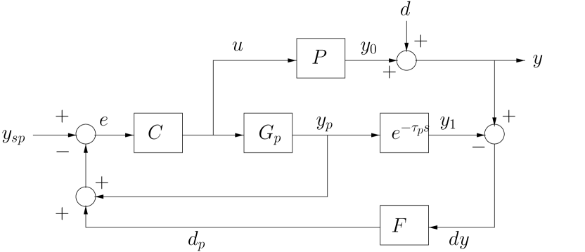
Figure 3: Feedback loop with Smith Predictor.

We first assume that the prediction model $P_{p}(s)=e^{-\tau_{p}s}G_{p}(s)$ matches the plant model $P(s)$ in (1), and use the following compensator settings:

$$C(s)=0.5(1+{1\over 40s}),\;\;\;F(s)={1\over 20s+1}.$$

By defining summation blocks and input and outputs names of systems, we obtain the closed-loop model $T_{SP}$ from the input signal $y_{sp}$ to the output signal $y$:

  s = tf(’s’);

  % LTI blocks
  P = exp(-93.9*s) * 5.6/(40.2*s+1);
  P.InputName = ’u’; P.OutputName = ’y’;

  Gp = 5.6/(40.2*s+1);
  Gp.InputName = ’u’; Gp.OutputName = ’yp’;

  Dp = exp(-93.9*s);
  Dp.InputName = ’yp’; Dp.OutputName = ’y1’;

  C = 0.5 * (1 + 1/(40*s));
  C.InputName = ’e’;  C.OutputName = ’u’;

  F = 1/(20*s+1);
  F.InputName = ’dy’; F.OutputName = ’dp’;

  % Sum blocks
  Sum1 = ss([1,-1,-1],’InputName’,...
         {’ysp’,’yp’,’dp’},’OutputName’,’e’);
  Sum2 = ss([1,-1],...
         ’InputN’,{’y’,’y1’},’OutputN’,’dy’);

  % Build interconnection model
  Tsp = connect(P,Gp,Dp,C,F,Sum1,Sum2,’ysp’,’y’);

We can also construct various types of connections such as in parallel and series (parallel and series); group systems by appending their inputs and outputs (append); form the linear fractional transformation (lft). Standard system operations are also valid for time delay systems such as addition, subtraction, multiplication, division.

After we represent our subsystems and connect with each other, we easily construct the closed-loop model with time delays. Our next goal is to analyze the characteristics of the resulting closed-loop models with visualizations and compute their system properties.

5 Time / Frequency Domain Analyses and Visualizations

We analyze a plant or a closed-loop model with various interconnections and systems to understand its characteristics and properties. By simulating its time-domain response to certain inputs such as a step or tracking signals, we observe its time-domain characteristics such as rise and settling times, overshoot. On the other hand, frequency domain analysis gives us information on, for example, gain and phase margins, bandwidth and resonant peak.

In Section 3, we obtained the closed-loop system $T_{PI}$ of the dead-time system (1) and PI controller and in Section 4 we constructed the closed-loop system $T_{SP}$ of the same plant and the Smith Predictor. We simulate the responses of $T_{PI}$ and $T_{SP}$ to the tracking signal, ref by the following commands:

% time and reference signal
time = 0:.1:2000;
ref = (time>=0 & time<1000)*4 + (time>=1000 & time<=2000)*8;

% compare responses
lsim(Tsp,Tpi,ref,time);

The resulting responses are shown in Figure 4 (on the left). Simulation results show that PI controller has a slower response time with oscillations and the Smith Predictor has better tracking performance.

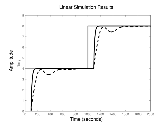
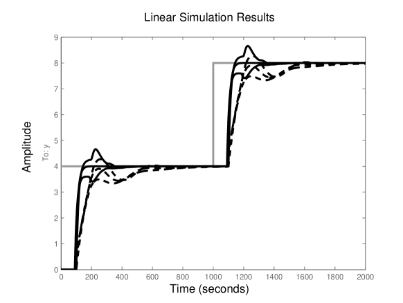
Figure 4: (left) Responses of the Smith Predictor (–) and PI (- -) to the reference signal (gray colored). (right) Robustness of the Smith Predictor (–) to Model Mismatch.

In practice, there is always a mismatch between the predicted and real plant models. We easily investigate robustness of our design to modeling uncertainties. For example, consider two perturbed plant models

$$P_{1}(s)=e^{-90s}{5\over 38s+1},\;\;P_{2}(s)=e^{-100s}{6\over 42s+1}\;.$$

To assess the Smith predictor robustness when the true plant model is $P_{1}(s)$ or $P_{2}(s)$ rather than the prediction model $P(s)$, simply bundle $P,P_{1},P_{2}$ into an LTI array, rebuild the closed-loop model(s), and replot the responses for the tracking signal:

  P1 = exp(-90*s) * 5/(38*s+1);         % perturbed plants
  P2 = exp(-100*s) * 6/(42*s+1);
  Plants = stack(1,P,P1,P2);            % bundle true and perturbed plants

  T = connect(Plants,Gp,Dp,C,F,Sum1,Sum2,’ysp’,’y’); % construct closed-loop

  lsim(T,Tpi,ref,time);                 % simulate closed-loop responses

The resulting responses in Figure 4 (on the right) show a slight performance degradation, but the Smith predictor still retains an edge over the pure PI design.

We obtain the closed-loop frequency responses for the nominal and perturbed plants by bode(T) and their visualizations as shown in Figure 5. Note that the phase behavior of systems with internal delays is quite different than systems with I / O delays.

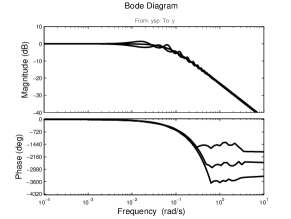
Figure 5: Closed-Loop Response from $y_{sp}$ to $y$.

We numerically compute the bandwidth of the responses by bandwidth(T) which returns $0.0695$, $0.0565$, $0.0767$. The gain and phase margins of the responses are calculated by [gm, pm] = margin(T) and their values are

$${\tt gm}=[1.0835;\ \ 1.1569;\ \ 1.0304],\quad{\tt pm}=[180;\ \ 180;\ \ 7.1433].$$

Other well-known frequency-domain based tools are also available for the GLTI class such as bandwidth, dcgain, nyquist, allmargin.

6 Controller Design

We analyzed the closed-loop characteristics of the given PI controller and Smith Predictor. Now we design a PID controller for finite dimensional and time delay plants using pidtune function in The Control System Toolbox and compare its performance with other controllers. This function aims to find a PID controller stabilizing the closed-loop system and to satisfy certain performance and robustness objectives. These objectives are tracking reference changes and suppressing disturbances as rapidly as possible; designing enough phase and margins for modeling errors or variations in system dynamics.

The algorithm for tuning PID controllers helps us meet these objectives by automatically tuning the PID gains to balance the response time as a performance objective and the stability margins as robustness objectives. By default, the algorithm chooses a crossover frequency (loop bandwidth) based upon the plant dynamics, and designs for a target phase margin of $60^{\circ}$.

We can approximate the dead-time system $P(s)$ by a finite dimensional transfer function $P_{a}(s)$ using the function pade based on Padé approximation. The function pidtune designs a PID controller $C_{a}(s)$ for the approximate finite dimensional plant and we obtain the closed-loop system for this controller by the following commands:

  Pa = pade(P,8);         % approximate 8th order plant
  Ca = pidtune(Pa,’pid’); % design PID for Pa
  Ta = feedback(P*Ca,1);  % closed-loop for Ca

Pidtune also designs a PID controller for time delay systems without any approximation,

  [Cpid,info] = pidtune(P,’pid’);   % design PID for P
  Tpid = feedback(P*Cpid,1);        % closed-loop for Cpid
  >> info

  info =

                  Stable: 1
      CrossoverFrequency: 0.0067
             PhaseMargin: 60.0000

As shown in returned info structure, the designed controller Cpid stabilizes the closed-loop and achieves $0.0067$ rad/sec crossover frequency and $60^{\circ}$ phase margin. The closed-loop step response Tpid of the controller Cpid is given Figure 6 (on the right with dashed line). Through step plot figure, we compute its transient response characteristics. The step response for this controller has $5.45\%$ overshoot, $136$ and $459$ seconds rise and settling times.

We compare the closed-loop responses of the Smith Predictor, the designed PID controllers for the approximate plant $P_{a}(s)$ and the original plant $P(s)$ by

  lsim(Tsp,Ta,Tpid,ref,time);

The responses in Figure 6 (on the left) show that the designed PID controller for the original plant offers a good compromise between the simplicity of the controller and good tracking performance compared to the Smith predictor.

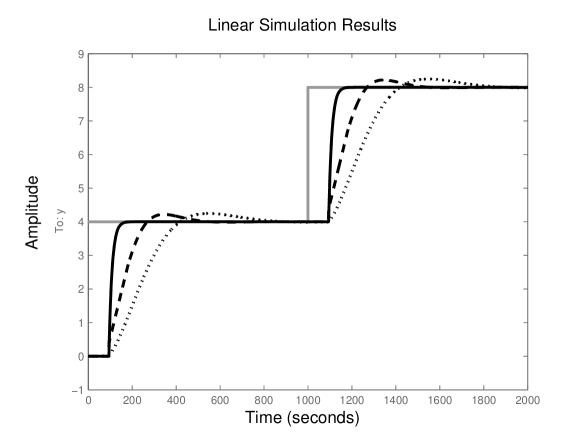
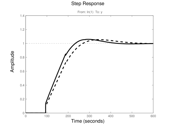
Figure 6: (left) Responses of the Smith Predictor (–), PID (- -) for $P(s)$ and PID (:) for $P_{a}(s)$ to the reference signal (gray colored). (right) Closed-loop step responses for the controllers Cpid (–) and Cpidf (- -).

We can fine tune the PID controller depending on design requirements. If faster response is required, we can increase the crossover frequency slightly and obtain the controller Cpidf by

Cpidf = pidtune(P,’pid’,0.0074);
Tpidf = feedback(P*Cpidf,1);
step(Tpid,Tpidf);

The closed-loop step responses for the controllers Cpid and Cpidf are shown Figure 6 (on the right). The new controller Cpidf has a faster response where its rise and settling times are $109$ and $394$ seconds, almost $20\%$ and $17\%$ faster than that of Cpid and its overshoot is slightly increased from $5.45\%$ to $5.89\%$.

7 Possible Enhancements in CACSD

We briefly summarized the available functionality in Control System Toolbox and we discuss possible enhancements for CACSD regarding time delay systems in this section. As illustrated before, most of the functions in Control System Toolbox are extended for time delay systems. We focus on three important numerical computations for time delay systems and discuss on-going research directions on these computations.

Stability of a time delay system

There are various numerical methods to determine the stability of LTI systems with constant delays Dugard1998 ; GuBook ; WimBook . One idea is to compute the characteristic roots when time delay is zero and to detect characteristic roots crossing the imaginary axis from zero delay to desired time delay and determine the stability of the time delay system. This approach is applicable to only systems with commensurate time delays and quasi-polynomial form is required. Another approach is to approximate the right-most characteristic roots in the complex plane using spectral methods further explained in the next section. The computational cost in this method depends on the number of discretization points for the time delay interval, i.e., from zero to maximum delay in the system. There are some heuristic methods to choose this number and they may result in poor choices at certain cases. Lyapunov theory is another tool to determine the stability of time delay systems. The results are conservative and in general the conservatism can be reduced in the expense of the computational cost of solving larger linear matrix inequalities. Most methods in the literature can not handle time delay systems with high orders.

System poles and zeros

The poles and zeros of time delay systems are computed by solving a nonlinear eigenvalue problem, essentially same problem to compute the characteristic roots of time delay systems. Therefore, approximating spectrum approach for characteristic roots is also used to compute system poles and zeros.

The computations are based on either discretization of the solution operator of a delay differential equation or the infinitesimal generator of the solution operator semigroup. The solution operator approach by linear-multi-step time integration for retarded type delay differential equations is given in Engelborghs2002 ; BIFTOOLManual20 . The infinitesimal generator approach discretizes the derivative in abstract delay differential equation by Runge-Kutta or linear multi-step methods and approximates into a matrix BredaSISC2005 ; BredaTraceDDE09 for retarded type delay differential equations with multiple discrete and distributed delays. Extensions to neutral type delay differential equations and mixed-type functional differential equations are done in BredaANM06 . Numerically stable implementation of spectral methods with some heuristics is given in TW596 .

The computation of system poles and zeros is closely connected with the nonlinear eigenvalue problem and an eigenvalue algorithm for this is presented in TW580 . A numerical method to compute all characteristic roots of a retarded or neutral quasi-polynomial on a large region in the complex-plane is proposed in TomasQPmR . The characteristic roots are calculated by finding the intersection of real and imaginary part of the characteristic equation on certain regions in complex-plane. This approach is further improved and accelerated by removing the regions outside of asymptotic chain roots in VZTAC09 . These methods consider the transfer function representation of delay differential equations which can be written as a ratio of quasi-polynomials. As noted in VZTAC09 , when delay differential equations have state-space representations, transforming these systems into transfer function representation is not numerically desired, therefore in this case discretization approaches may be preferred.

${\cal H}_{\infty}$ and $\mathcal{H}_{2}$ norms

The computation of ${\cal H}_{\infty}$ and $\mathcal{H}_{2}$ norms of time delay systems are quite new research topics and there are few research papers on these topics. Similar to the computation of system poles and zeros, ${\cal H}_{\infty}$ norm computation is reduced solving a nonlinear eigenvalue problem where the recent developments are applicable, Michiels2010 . The computation of $\mathcal{H}_{2}$ norm requires solving the delay Lyapunov equation, JarlebringTAC11 .

Note that all three computation methods are mainly used for analysis of time delay systems. Another challenging task is to design controllers and to extend classical control methods to time delay systems such as LQG, $\mathcal{H}_{2}$ control, ${\cal H}_{\infty}$ control, root-locus technique, model reduction methods.

There are continuing research efforts to solve these problems such as Vanbiervliet2011IJC ; Gumussoy2011SICON ; Gumussoy2012AUT ; TW602 . The remaining main task is to determine numerically stable algorithms to solve control design problems for high dimensional plant with the least user interactions.

8 Concluding Remarks

We have shown that the GLTI class is suitable for computer-aided manipulation of time delay systems. We discussed various representations and interconnections of time delay systems on MATLAB. We presented the MATLAB functionality to analyze and design control systems with delays, regardless of the control structure and number of delays. Most Control System Toolbox functions have been extended to work on GLTI models, all this without additional complexity or new syntax for the user. We hope that these new tools will facilitate the design of control systems with delays and bring new insights into their behavior.

References

- (1) Atay, F.M. (ed.): Complex time delay Systems: Theory and Applications. Understanding Complex Systems. Springer (2010)
- (2) Breda, D., Maset, S., Vermiglio, R.: Pseudospectral differencing methods for characteristic roots of delay differential equations. SIAM Journal on Scientific Computing 27(2), 482–495 (2005)
- (3) Breda, D., Maset, S., Vermiglio, R.: Pseudospectral approximation of eigenvalues of derivative operators with non-local boundary conditions. Applied Numerical Mathematics 56(3-4), 318–331 (2006)
- (4) Breda, D., Maset, S., Vermiglio, R.: TRACE-DDE: a Tool for Robust Analysis and Characteristic Equations for Delay Differential Equations, Lecture Notes in Control and Information Sciences, vol. 388. Springer (2009)
- (5) Dugard, L., Verriest, E. (eds.): Stability and control of time delay systems, Lecture Notes in Control and Information Sciences, vol. 228. Springer-Verlag (1998)
- (6) Engelborghs, K., Luzyanina, T., Samaey, G.: DDE-BIFTOOL V. 2.00: a Matlab Package for Bifurcation Analysis of Delay Differential Equations. Technical Report TW330, Department of Computer Science, K. U. Leuven, Leuven, Belgium (2001)
- (7) Engelborghs, K., Roose, D.: On stability of LMS methods and characteristic roots of delay differential equations. SIAM Journal on Numerical Analysis 40(2), 629–650 (2002)
- (8) Enright, W.H., Hayashi, H.: A delay differential equation solver based on a continuous rungekutta method with defect control. Numerical Algorithms 16, 349–364 (1997)
- (9) Erneux, T.: Applied delay differential equations. Surveys and tutorials in the applied mathematical sciences. Springer (2009)
- (10) Gahinet, P., Shampine, L.F.: Software for modeling and analysis of linear systems with delays. In: Proceedings of the American Control Conference (2004)
- (11) Gu, K., Kharitonov, V., Chen, J.: Stability of time delay systems. Birkhäuser, Boston, MA (2003)
- (12) Gumussoy, S., Michiels, W.: Fixed-Order H-infinity Control for Interconnected Systems using Delay Differential Algebraic Equations. SIAM Journal on Control and Optimization 49(2), 2212–2238 (2011)
- (13) Gumussoy, S., Michiels, W.: Root Locus for SISO Dead-Time Systems: A Continuation Based Approach. Automatica 48(3), 480–489 (2012)
- (14) Gumussoy, S., Eryilmaz, B., Gahinet, P.: Working with Time-Delay Systems in MATLAB. 10th IFAC Workshop on Time Delay Systems, June 22-24, Northeastern University, USA, 2012. IFAC-PapersOnLine, 108–113, doi: 10.3182/20120622-3-US-4021.00041, 2012.
- (15) Hairer, E., Wanner, G.: RETARD: Software for delay differential equations. http://unige.ch/~hairer/software.html (1995)
- (16) Ingimundarson, A., Hagglund, T.: Robust tuning procedures of dead-time compensating controllers. Control Engineering Practice 9, 1195–1208 (2001)
- (17) Jarlebring, E., Damm, T., Michiels, W.: Model reduction of time delay systems using position balancing and delay Lyapunov equations. Technical Report TW602, Department of Computer Science, K. U. Leuven, Leuven, Belgium (2011)
- (18) Jarlebring, E., Michiels, W., Meerbergen, K.: A linear eigenvalue algorithm for the nonlinear eigenvalue problem. Technical Report TW580, Department of Computer Science, K. U. Leuven, Leuven, Belgium (2011)
- (19) Jarlebring, E., Vanbiervliet, J., Michiels, W.: Characterizing and computing the L2 norm of time delay systems by solving the delay Lyapunov equation. IEEE Transactions on Automatic Control 56, 814–825 (2011)
- (20) Michiels, W., Gumussoy, S.: Characterization and computation of H-infinity norms of time delay systems. SIAM Journal on Matrix Analysis and Applications 31(4), 2093–2115 (2010)
- (21) Michiels, W., Niculescu, S.I.: Stability and stabilization of time delay systems. An eigenvalue based approach, Advances in design and control, vol. 12. SIAM, Philadelphia (2007)
- (22) Niculescu, S.I.: Delay effects on stability: A robust control approach, Lecture notes in control and information sciences, vol. 269. Springer-Verlag, London (2001)
- (23) Skogestad, S., Postlethwaite, I.: Multivariable Feedback Control. John Wiley (1996)
- (24) Control System Toolbox: MathWorks Inc., Natick (2011)
- (25) Vanbiervliet, J., Michiels, W., Jarlebring, E.: Using spectral discretization for the optimal H2 design of time delay systems. International Journal of Control 84(2), 228–241 (2011)
- (26) Vyhlídal, T., Zítek, P.: Quasipolynomial mapping based rootfinder for analysis of time delay systems. In: Proceedings of the 4th IFAC workshop on Time Delay Systems, pp. 227–232. Rocquencourt, France (2003)
- (27) Vyhlídal, T., Zítek, P.: Mapping based algorithm for large-scale computation of quasi-polynomial zeros. IEEE Transactions on Automatic Control 54(1), 171–177 (2009)
- (28) Wu, Z., Michiels, W.: Reliably computing all characteristic roots of delay differential equations in a given right half plane using a spectral method. Technical Report TW596, Department of Computer Science, K. U. Leuven, Leuven, Belgium (2011)