Nonadiabatic particle and energy pump at strong system-reservoir coupling

Abstract

We study the dynamics of electron and energy currents in a nonadiabatic pump. The pump is a quantum dot nanojunction with time-varying gate potential and tunnel couplings to the leads. The leads are unbiased and maintained at the same temperature and chemical potential. We find that synchronized variations of the gate and tunnel couplings can pump electrons and energy from the left to the right lead. Inspired by quantum heat engines, we devise a four-stroke operating protocol that can optimally pump energy and hence, we investigate energy transfer and the coefficient of performance of the device. We compare our device to a two-stroke pump and find that the latter’s lower performance is due to the bi-directional flow of energy currents resulting in low net energy currents. The performance of our four-stroke pump can be improved, up to a point, by increasing the net energy carried by the pumped electrons through energy charging via the gate potential. This is achieved by increasing the durations of energy charging and discharging strokes in the pump’s protocol. However, despite the large energy output for long charging and discharging strokes, the energy required to maintain the strokes become large too resulting in a stagnant pump performance. Our pump operates effectively only in the strong lead coupling regime and becomes a dud in the weak coupling regime due to the net output energy flowing in the reverse direction. We use nonequilibirum Green’s functions techniques to calculate the currents and capture the effects of strong lead-channel coupling exactly while simultaneously incorporating three time-varying parameters. Results from our work could aid in the design of high-performance quantum pumps.

I Introduction

Control of the flow of energy in nanoscale systems is important in an era where the generation of heat in high-speed electronic devices is a major problem. Phononics Li et al. (2012), the study of the flow of energy carried by phonons in quantum systems, has led to the idea of quantum heat pumps that can transport energy even against a temperature bias Pekola et al. (2007). In electronic transport, an analogous device called an electron pump, which can be a junction that uses gate potentials to propagate electrons without the action of a source-drain bias, has been studied extensively in both the adiabatic Thouless (1983); Brouwer (1998); Switkes et al. (1999); Entin-Wohlman et al. (2002); Moskalets and Büttiker (2002); Blumenthal et al. (2007); Riwar et al. (2013); Ludovico et al. (2016) and the nonadiabatic Strass et al. (2005); Braun and Burkard (2008); Moskalets and Büttiker (2008); Cavaliere et al. (2009); Croy and Saalmann (2012); Roche et al. (2013); Kaestner and Kashcheyevs (2015); Haughian et al. (2017); Wenz et al. (2016); Yamahata et al. (2017) regimes. The pumping of energy carried by electrons has also been studied either in the weak system-environment coupling regime Segal and Nitzan (2006) or in the adiabatic regime Humphrey et al. (2002); Ren et al. (2010), with the exception of specialized coherent transport models that have been studied in the non-adiabatic regime Rey et al. (2007).

Heat engines are thermodynamic devices that can transform input heat into work by following a specific operating protocol. Heat pumps, on the other hand, require an input of work to propagate heat. Heat pumps are, therefore, thermodynamic engines operated under a time-reverse protocol. It is thus natural to investigate the role of thermodynamic principles in enhancing the performance of heat pumps Ren et al. (2010); Potanina et al. (2019). Inspired by heat engines that follow a four-stroke protocol Uzdin et al. (2015), we design an electronic device that can pump energy to a predefined direction in the absence of temperature and voltage bias. The device operates in the non-adiabatic regime and is always strongly coupled to leads, in contrast to traditional adiabatic heat pumps that are weakly coupled to heat baths. In order to fully capture the physics of this nontrivial operational regime, we employ nonequilibrium Green’s functions techniques Arrachea (2005); Croy and Saalmann (2012); Daré and Lombardo (2016). Our approach allows us to explore weak to strong system-environment coupling strengths and we find that even though we are able to pump unidirectional charge for any coupling strength, the unidirectional energy pumping occurs only in the strong coupling regime. In the nonadiabatic regime, we find values of the parameters wherein the output energy is maximum and accompanied by a coefficient of performance that is close to the maximum value too. Moreover, the device that we are proposing is feasible with current technology Roche et al. (2013); Kaestner and Kashcheyevs (2015); Haughian et al. (2017); Yamahata et al. (2017) and hence, our results can be scrutinized experimentally.

Our paper is sectioned as follows. In Sec. II we discuss the model of our proposed four-stroke non-adiabatic pump. We describe the four strokes of our device and contrast its performance with a minimal two-stroke pump. In Sec. III we show how we calculate the electron and energy currents using nonequilibrium Green’s functions in the time domain. In Sec. IV we present and discuss our results. The summary and conclusion are in Sec. V.

II Modeling the Device

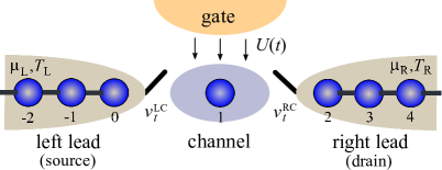
Figure 1: Electrons are pumped from the left lead to the right by dynamically varying the tunnel couplings between the channel and the leads, i.e., the $v_{t}^{\rm LC}$ and $v_{t}^{\rm RC}$, and the gate potential $U(t)$ acting on the channel. The left and right leads have chemical potentials $\mu_{\rm L}$ and $\mu_{\rm R}$ and temperatures $T_{\rm L}$ and $T_{\rm R}$.

We consider a central one-site channel, tuned by a time-varying gate potential, coupled to left (the source) and right (the drain) leads, as illustrated in Fig. 1. The tunnel couplings between the channel and the leads can also be tuned dynamically and independently via additional gate potentials. In order to realize a pump, the variations of the gate potential and the tunnel couplings are synchronized according to a specific operating protocol (described below) so that electrons are unidirectionally pumped from the left to the right lead, even in the absence of a source-drain bias voltage. We model the device using the tight-binding approximation. The Hamiltonians for the leads are

$$\begin{split}H^{\rm L}&=\sum_{k}\varepsilon_{k}^{\rm L}a_{k}^{\dagger}a_{k}+\sum_{k<j}v_{kj}^{\rm L}\left(a_{k}^{\dagger}a_{j}+a_{j}^{\dagger}a_{k}\right),\\ H^{\rm R}&=\sum_{k}\varepsilon_{k}^{\rm R}b_{k}^{\dagger}b_{k}+\sum_{k<j}v_{kj}^{\rm R}\left(b_{k}^{\dagger}b_{j}+b_{j}^{\dagger}b_{k}\right),\end{split}$$ (1)

where $a_{k}^{\dagger}$ ($b_{k}^{\dagger}$) and $a_{k}$ ($b_{k}$) are the spinless fermionic creation and annihilation operators at site $k$ in the left (right) lead, $\varepsilon_{k}^{\rm L}$ ($\varepsilon_{k}^{\rm R}$) are the on-site energies in the leads, and $v_{kj}^{\rm L}$ and $v_{kj}^{\rm R}$ are the nearest-neighbour hopping parameters. Sites in the left lead are labelled $k\in(-\infty,0]$, while $k\in[2,\infty)$ are the labels of sites in the right lead. The single-site central channel Hamiltonian contains

$$H_{0}^{\rm C}=\varepsilon_{1}^{\rm C}c_{1}^{\dagger}c_{1}\quad{\rm and}\quad H_{t}^{\rm C}=U\!(t)\,c_{1}^{\dagger}c_{1},$$ (2)

where $c_{1}^{\dagger}$ and $c_{1}$ are the spinless fermionic creation and annihilation operators at site $1$, $\varepsilon_{1}^{\rm C}$ is the on-site energy at the same site, and $U\!(t)$ is the time-varying gate potential. The lead-channel coupling Hamiltonians are separated into stationary

$$\begin{split}H_{0}^{\rm LC}&=v_{01}^{\rm LC}\left(a_{0}^{\dagger}c_{1}+c_{1}^{\dagger}a_{0}\right),\\ H_{0}^{\rm RC}&=v_{21}^{\rm RC}\left(b_{2}^{\dagger}c_{1}+c_{1}^{\dagger}b_{2}\right),\end{split}$$ (3)

and time-dependent parts

$$\begin{split}H_{t}^{\rm LC}&=v_{01}^{\rm LC}\!(t)\left(a_{0}^{\dagger}c_{1}+c_{1}^{\dagger}a_{0}\right),\\ H_{t}^{\rm RC}&=v_{21}^{\rm RC}\!(t)\left(b_{2}^{\dagger}c_{1}+c_{1}^{\dagger}b_{2}\right).\end{split}$$ (4)

The time-varying $v_{01}^{\rm LC}\!(t)$ and $v_{21}^{\rm RC}\!(t)$ can increase or decrease the strength of the couplings between the channel and the leads. We set all of the hopping parameters to be space-symmetric, i.e., $v_{jk}=v_{kj}$. The total Hamiltonian is then the sum of the stationary and the time-varying parts, i.e., $H=H_{0}+H_{t}$, where $H_{0}=H^{\rm L}+H^{\rm R}+H_{0}^{\rm C}+H_{0}^{\rm LC}+H_{0}^{\rm RC}$ is the stationary part and $H_{t}=H_{t}^{\rm C}+H_{t}^{\rm LC}+H_{t}^{\rm RC}$ is the time-dependent part.

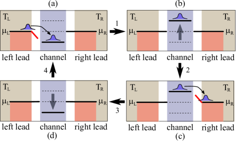
Figure 2: Illustration of the four strokes of the pump cycle. Electrons are represented by (blue) wavepackets. (a) The left-channel coupling (in red) allows more electrons from the left lead to flow into the channel. (b) The left-channel coupling decreases and the gate potential in the channel is raised thereby trapping some electrons within the channel. (c) The right-channel coupling (in red) allows electrons to flow out to the right lead. (d) The right-channel coupling decreases and the gate potential is lowered thereby restricting the flow of electrons into or out of the channel. The chemical potentials and temperatures of the two leads are the same.

In order for the device to function as a pump, the time-dependence of the gate potential $U\!(t)$ and the tunnel couplings $v_{01}^{\rm LC}\!(t)$ and $v_{21}^{\rm RC}\!(t)$ must be synchronized. Inspired by four-stroke quantum heat engines such as the quantum Otto engine Uzdin et al. (2015), we design a four-stroke operating protocol as shown in Fig. 2. These four strokes are:

1. Stroke a: Transport stroke. The channel and the left lead are coupled, the gate potential lowers the level in the channel, and electrons from the left lead can flow into the channel.

2. Stroke b: Energy charging stroke. The left lead-channel coupling is abruptly decreased and, simultaneously, the gate potential raises the level in the channel. Electrons in the channel gain energy because of the raised level.

3. Stroke c: Transport stroke. The channel and the right lead are coupled, the gate continues to raise the level in the channel, and electrons in the channel can flow to the right lead.

4. Stroke d: Energy discharging stroke. The right lead-channel coupling is abruptly decreased and, simultaneously, the gate lowers the energy level in the channel.

The cycle then repeats and at no point in time are the channel and leads disconnected. The driving potentials perform work on the device, pushing the device into a nonequilibrium state which then allows us to pump electrons and energy despite the absence of temperature and voltage bias between the leads. There have been several studies that have investigated adiabatic pumping and the weak system-environment coupling regimes of quantum pumps Thouless (1983); Brouwer (1998); Zhou et al. (1999); Thingna et al. (2014), with each attempt employing an approximate scheme to a specific physical time-dependent protocol. In the rest of this work, we will present an exact formulation to treat nonadiabatic pumping with three time-dependent components in a four-stroke operating protocol and contrast its performance with a minimal two-stroke protocol that comprises of strokes a and c only (see Fig. 2).

The energy gained by the pumped electrons in one cycle can be used to run another device such as a quantum motor Fernández-Alcázar et al. (2017) to convert electrical energy into mechanical energy. We can determine the energy current of the pumped electrons from the rate of change of the energy in each lead. The energy current Cuansing and Wang (2010); Thingna et al. (2012); Wang et al. (2014); Esposito et al. (2015), traditionally known as the heat current, out of the left lead is

$$J^{\rm L}(t)=\left\langle-\frac{dH^{\rm L}}{dt}\right\rangle=-\frac{i}{\hbar}\left\langle\left[H,H^{\rm L}\right]\right\rangle,$$ (5)

where the Heisenberg equation of motion is used in the second equality and considering that $H^{\rm L}$ has no explicit time dependence. The negative sign indicates that the current is positive if it is flowing to the right. The commutator between $H$ and $H^{\rm L}$ can be derived by using the fermionic anti-commutation rules, i.e., $\{a_{k}^{\dagger},a_{j}\}=\{a_{k},a_{j}^{\dagger}\}=\delta_{kj}$ and zero otherwise. Thus, we get

$$\begin{split}J^{\rm L}(t)=\,&2\,\varepsilon_{0}^{\rm L}\left[v_{01}^{\rm LC}+v_{01}^{\rm LC}\!(t)\right]{\rm Re}\!\left[G_{10}^{{\rm CL},<}(t,t)\right]\\ &+2\,v^{\rm L}_{-1\,0}\left[v^{\rm LC}_{01}+v_{01}^{\rm LC}\!(t)\right]{\rm Re}\!\left[G^{{\rm CL},<}_{1\,-1}(t,t)\right],\end{split}$$ (6)

where the lesser channel left-lead (${\rm CL}$) nonequilibrium Green’s function is defined as

$$G_{jk}^{{\rm CL},<}(t_{1},t_{2})=\frac{i}{\hbar}\left\langle a_{k}^{\dagger}(t_{2})\,c_{j}(t_{1})\right\rangle$$ (7)

and ${\rm Re}[\,]$ refers to the real part. The energy current flowing into the right lead, $J^{\rm R}(t)$, is similarly determined. The result has the same form as Eq. (6) but with the replacement of all the superscripts ${\rm L}$, the subscripts $0$ and $-1$, and the operator $a_{k}$ by the superscripts ${\rm R}$, subscripts $2$ and $3$, and the operator $b_{k}$, respectively. There is also an overall negative sign due to the reversed direction of the current in the definition. To be consistent with $J^{\rm L}(t)$, a positive $J^{\rm R}(t)$ means a current that is moving to the right lead. The net energy current flowing across the device is $J_{\rm net}(t)=J^{\rm L}(t)+J^{\rm R}(t)$.

The electric current flowing out of the left lead follows the time rate of change of the number of electrons in the lead, where the number operator in the left lead is $N^{\rm L}=\sum_{k}a^{\dagger}_{k}a_{k}$,

$$\begin{split}I^{\rm L}(t)&=\left\langle-q\frac{dN^{\rm L}}{dt}\right\rangle=-\frac{iq}{\hbar}\left\langle\left[H,N^{\rm L}\right]\right\rangle\\ &=2q\left[v^{\rm LC}_{01}+v_{01}^{\rm LC}\!(t)\right]{\rm Re}\!\left[G^{{\rm CL},<}_{10}(t,t)\right],\end{split}$$ (8)

where $q$ is the electron charge. Notice that $I^{\rm L}(t)$ is proportional only to the first term of the energy current $J^{\rm L}(t)$ appearing in Eq. (6) and hence, in general, the pumping of electrons does not guarantee the pumping of energy, and vice versa. The electric current flowing into the right lead, $I^{\rm R}(t)$, is obtained using the same replacements described below Eq. (7). Consequently, the net electric current is $I_{\rm net}(t)=I^{\rm L}(t)+I^{\rm R}(t)$.

The coefficient of performance, ${\rm COP}$, of the pump can be determined from the ratio of the output energy and the net energy needed to run the device,

$${\rm COP}=\frac{E_{\rm out}}{E_{\rm in}},$$ (9)

where the output and input energies are

$$\begin{split}E_{\rm out}&=\int_{\rm cycle}J_{\rm net}(t)\,dt,\\ E_{\rm in}&=\frac{1}{T}\int_{\rm cycle}\left(\left|\langle H_{t}^{\rm C}\rangle\right|+\left|\langle H_{t}^{\rm LC}\rangle\right|+\left|\langle H_{t}^{\rm RC}\rangle\right|\right)dt.\end{split}$$ (10)

The integrals are over one pumping cycle and $T$ is the cycle period. For $E_{\rm in}$, which is always positive, we need the values of the energy that the time-varying gate supplies,

$$\begin{split}\left|\langle H_{t}^{\rm C}\rangle\right|&=\left|\left\langle U(t)\,c_{1}^{\dagger}(t)c_{1}(t)\right\rangle\right|\\ &=\hbar\,U(t)\sqrt{{\rm Re}\!\left[G_{11}^{{\rm CC},<}(t,t)\right]^{2}+{\rm Im}\!\left[G_{11}^{{\rm CC},<}(t,t)\right]^{2}},\end{split}$$ (11)

where ${\rm Im}[\,]$ refers to the imaginary part and the Green’s function

$$G_{11}^{{\rm CC},<}(t_{1},t_{2})=\frac{i}{\hbar}\left\langle c_{1}^{\dagger}(t_{2})c_{1}(t_{1})\right\rangle$$ (12)

and the energies supplied by the time-varying lead-channel couplings,

$$\begin{split}\left|\langle H_{t}^{\rm LC}\rangle\right|&=\left|2\hbar\,v_{t}^{\rm LC}\,{\rm Im}\left[G_{10}^{{\rm CL},<}(t,t)\right]\right|,\\ \left|\langle H_{t}^{\rm RC}\rangle\right|&=\left|2\hbar\,v_{t}^{\rm RC}\,{\rm Im}\left[G_{12}^{{\rm CR},<}(t,t)\right]\right|.\end{split}$$ (13)

$E_{\rm in}$ is therefore the total amount of input energy per cycle needed to operate the device.

III Nonequilibrium Green’s functions

We use the Schwinger-Keldysh formalism Pastawski (1992); Jauho et al. (1994); Haug and Jauho (2008); Stefanucci and van Leeuwen (2013) to determine the lesser nonequilibrium Green’s functions. The ${\rm CL}$ contour-ordered Green’s function is defined as

$$G_{jk}^{\rm CL}(\tau_{1},\tau_{2})=-\frac{i}{\hbar}\left\langle{\rm T}_{c}\,c_{j}(\tau_{1})a_{k}^{\dagger}(\tau_{2})\right\rangle,$$ (14)

where ${\rm T}_{c}$ is the contour-ordering operator along the Keldysh contour $c$ shown in Fig. 3(b).

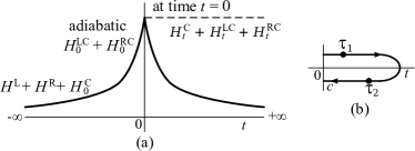
Figure 3: Illustrations of (a) how the various terms in the Hamiltonian are switched on and (b) the Keldysh contour $c$ with contour time variables $\tau_{1}$ and $\tau_{2}$. The contour begins at $0$, goes to $t$, and then back to $0$.

Terms in the total Hamiltonian are switched on according to the scheme shown in Fig. 3(a). At time far in the past, the channel and the two leads are initially considered to be uncoupled and at their own equilibrium states. The lead-channel couplings are then adiabatically switched on in such a way that at time $t=0$ the coupled system is at the steady state. The time-varying components $H_{t}=H^{\rm C}_{t}+H^{\rm LC}_{t}+H^{\rm RC}_{t}$ are then abruptly switched on at time $t=0$.

In the interaction picture, the contour-ordered Green’s function takes the form

$$G_{jk}^{\rm CL}(\tau_{1},\tau_{2})=-\frac{i}{\hbar}\left\langle{\rm T}_{c}\,e^{-\frac{i}{\hbar}\int_{c}H_{t}(\tau^{\prime})d\tau^{\prime}}c_{j}(\tau_{1})\,a_{k}^{\dagger}(\tau_{2})\right\rangle_{0},$$ (15)

where the subscript $0$ implies that the average is taken with respect to the steady state. Steady-state Green’s functions can be determined exactly (see below), even in the strong leads-channel coupling regime, because the associated stationary Hamiltonian $H_{0}$ is purely quadratic. The contour-ordered Green’s function in Eq. (15) is then determined via a diagrammatic perturbative expansion and the result is a series of terms containing steady-state Green’s functions and their integrals. We would like to note that although the time-dependent perturbations $H^{\rm C}_{t}+H^{\rm LC}_{t}+H^{\rm RC}_{t}$ are quadratic in form, expanding the contour-ordered Green’s function results in high-order diagrams that cannot be accounted by an iterative equation. In order to arrive at an iterative Dyson equation, we make an approximation by setting the amplitudes of the time-varying parameters $U\!(t)$, $v_{01}^{\rm LC}\!(t)$, and $v_{21}^{\rm RC}\!(t)$ to be much smaller than the on-site energy $\varepsilon_{1}$ and stationary hopping parameters $v_{01}^{\rm LC}$ and $v_{21}^{\rm RC}$. The diagram representations of the Green’s functions are shown in Fig. 4(a) and (b) and the resulting approximate iterative diagram equation is shown in Fig. 4(c).

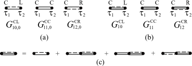
Figure 4: Diagram representations of (a) the steady-state Green’s functions, (b) the nonequilibrium Green’s functions, and (c) the approximate iterative equation for $G_{10}^{\rm CL}(\tau_{1},\tau_{2})$. Each vertex implies either a $U$, $v_{t}^{\rm LC}$, or $v_{t}^{\rm RC}$ coupling strength depending on the Green’s function immediately to the left of it. All internal contour time variables are integrated out.

An alternative approach is to switch on the time-dependent perturbations at a time when the channel and the leads are still uncoupled. In this case the system is not in a steady state and the perturbation expansion of the contour-ordered Green’s function would lead to terms based on the equilibrium Green’s functions of the leads and the channel. Although an exact iterative equation can be constructed from this approach, it requires knowledge of the channel’s temperature and chemical potential, which are not well-defined due to the channel being finite. In contrast, in the approach that we use, there is no such requirement when the contour-ordered Green’s function is expressed in terms of steady-state Green’s functions.

Similar approximate iterative diagram equations can be derived for $G_{jk}^{\rm CR}$ and $G_{jk}^{\rm CC}$. The corresponding iterative equations for these contour-ordered Green’s functions are

$$\begin{split}G_{jk}^{\gamma}(\tau_{1},\tau_{2})=&~{}G_{jk,0}^{\gamma}(\tau_{1},\tau_{2})\\ &~{}+\int_{c}d\tau^{\prime}\,B_{j1,0}^{\rm C}(\tau_{1},\tau^{\prime})\,G_{1k}^{\gamma}(\tau^{\prime},\tau_{2}),\end{split}$$ (16)

where $\gamma={\rm CL},{\rm CC},{\rm CR}$, the subscript $0$ indicates the steady-state version of the Green’s function, the integrals are along the Keldysh contour, and

$$\begin{split}B_{j1,0}^{\rm C}(\tau,\tau^{\prime})=&~{}G_{j0,0}^{\rm CL}(\tau,\tau^{\prime})\,v_{01}^{\rm LC}(\tau^{\prime})+G_{j1,0}^{\rm CC}(\tau,\tau^{\prime})\,U_{1}(\tau^{\prime})\\ &+G_{j2,0}^{\rm CR}(\tau,\tau^{\prime})\,v_{21}^{\rm RC}(\tau^{\prime}).\end{split}$$ (17)

Notice that only the steady-state versions of the Green’s functions appear in Eq. (17). Applying analytic continuation and Langreth’s theorem to the contour-ordered Green’s function in Eq. (16), the retarded and advanced nonequilibrium Green’s functions in real time variables are

$$\begin{split}G_{jk}^{\gamma,\alpha}(t_{1},t_{2})=&~{}G_{jk,0}^{\gamma,\alpha}(t_{1},t_{2})\\ &~{}+\int_{0}^{t}dt^{\prime}\,B_{j1,0}^{{\rm C},\alpha}(t_{1},t^{\prime})\,G_{1k}^{\gamma,\alpha}(t^{\prime},t_{2}),\end{split}$$ (18)

where $\alpha=r,a$. Also from the Langreth rules, the lesser nonequilibrium Green’s functions are

$$\begin{split}G_{jk}^{\gamma,<}&(t_{1},t_{2})=G_{jk,0}^{\gamma,<}(t_{1},t_{2})\\ +&~{}\int_{0}^{t}dt^{\prime}\,B_{j1}^{{\rm C},r}(t_{1},t^{\prime})\,G_{1k,0}^{\gamma,<}(t^{\prime},t_{2})\\ +&~{}\int_{0}^{t}dt^{\prime}\,B_{j1,0}^{{\rm C},<}(t_{1},t^{\prime})\,G_{1k}^{\gamma,a}(t^{\prime},t_{2})\\ +&~{}\int_{0}^{t}dt^{\prime}\int_{0}^{t}dt^{\prime\prime}\,B_{j1}^{{\rm C},r}(t_{1},t^{\prime})\,B_{11,0}^{{\rm C},<}(t^{\prime},t^{\prime\prime})\,G_{1k}^{\gamma,a}(t^{\prime\prime},t_{2}),\end{split}$$ (19)

where $\gamma$ is either ${\rm CL}$ or ${\rm CR}$ and

$$\begin{split}B_{j1}^{{\rm C},\alpha}(t,t^{\prime})=&~{}G_{j0}^{{\rm CL},\alpha}(t,t^{\prime})\,v_{01}^{\rm LC}(t^{\prime})+G_{j1}^{{\rm CC},\alpha}(t,t^{\prime})\,U_{1}(t^{\prime})\\ &~{}+G_{j2}^{{\rm CR},\alpha}(t,t^{\prime})\,v_{21}^{\rm RC}(t^{\prime}),\end{split}$$ (20)

while the $B_{j1,0}^{{\rm C},\alpha}(t,t^{\prime})$ are the corresponding steady-state versions. Note that the Green’s functions in Eq. (19) are the lesser nonequilibrium Green’s functions needed to determine the currents.

To numerically determine the retarded and advanced nonequilibrium Green’s functions in Eq. (18), we discretize the time variable and re-express the integral as a sum Cuansing (2017). Steady-state Green’s functions are determined from the adiabatic switch-on of $H_{0}^{\rm LC}+H_{0}^{\rm RC}$, as shown in Fig. 3(a), and leads to an exact iterative Dyson equation. For the ${\rm CC}$ steady-state Green’s function, we get

$$\begin{split}G_{11,0}^{\rm CC}&(\tau_{1},\tau_{2})=g_{11}^{\rm C}(\tau_{1},\tau_{2})\\ &+\int_{c}d\tau^{\prime}\int_{c}d\tau^{\prime\prime}\,g_{11}^{\rm C}(\tau_{1},\tau^{\prime})\,\Sigma_{11}^{\rm C}(\tau^{\prime},\tau^{\prime\prime})\,G_{11,0}^{\rm CC}(\tau^{\prime\prime},\tau_{2}),\end{split}$$ (21)

where $g_{11}^{\rm C}$ is the equilibrium Green’s function of the channel. The self-energy is

$$\Sigma_{11}^{\rm C}(\tau,\tau^{\prime})=v_{10}^{\rm CL}\,g_{00}^{\rm L}(\tau,\tau^{\prime})\,v_{01}^{\rm LC}+v_{12}^{\rm CR}\,g_{22}^{\rm R}(\tau,\tau^{\prime})\,v_{21}^{\rm RC},$$ (22)

and $g_{00}^{\rm L}$ and $g_{22}^{\rm R}$ are the equilibrium Green’s functions of site $0$ in the left lead and site $2$ in the right lead, respectively. Using analytic continuation and Langreth’s theorem would lead to expressions for the retarded, advanced, and lesser ${\rm CC}$ steady-state Green’s functions. Furthermore, since time-translation invariance is satisfied in the steady state, the steady-state Green’s functions are simply functions of the difference between two times and we take their Fourier transforms into the energy domain to obtain

$$\begin{split}G_{11,0}^{{\rm CC},r}(E)&=\left[\left(E+i\eta\right)-\varepsilon_{1}^{\rm C}-\Sigma_{11}^{{\rm C},r}(E)\right]^{-1},\\ G_{11,0}^{{\rm CC},a}(E)&=\left(G_{11,0}^{{\rm CC},r}(E)\right)^{\ast},\\ G_{11,0}^{{\rm CC},<}(E)&=G_{11,0}^{{\rm CC},r}(E)\,\Sigma_{11}^{{\rm C},<}(E)\,G_{11,0}^{{\rm CC},a}(E).\end{split}$$ (23)

These ${\rm CC}$ steady-state Green’s functions are often used in steady-state quantum transport calculations Haug and Jauho (2008); Stefanucci and van Leeuwen (2013). Following the same procedure, the ${\rm CL}$ steady-state Green’s functions are

$$\begin{split}G_{jk,0}^{{\rm CL},r}(E)=&~{}G_{j1,0}^{{\rm CC},r}(E)\,v_{10}^{\rm CL}\,g_{0k}^{{\rm L},r}(E),\\ G_{jk,0}^{{\rm CL},a}(E)=&~{}\left(G_{jk,0}^{{\rm CL},r}(E)\right)^{\ast},\\ G_{jk,0}^{{\rm CL},<}(E)=&~{}G_{j1,0}^{{\rm CC},r}(E)\,v_{10}^{\rm CL}\,g_{0k}^{{\rm L},<}(E)\\ &~{}~{}~{}+G_{j1,0}^{{\rm CC},r}(E)\,\Sigma_{11}^{{\rm C},<}(E)\,G_{1k,0}^{{\rm CL},a}(E).\end{split}$$ (24)

Note that the Fourier transforms into the time domain of the steady-state Green’s functions are required in the calculation of the time-dependent nonequilibrium Green’s functions Cuansing (2017).

The equilibrium Green’s functions can be derived from the equation of motion of the free leads. For the left lead, we find the retarded Green’s functions to be

$$\begin{split}g_{00}^{{\rm L},r}(E)=&~{}2\frac{\left(E+i\eta\right)-\varepsilon}{v^{2}}\pm 2\,i\,\frac{\sqrt{v^{2}-\left(\varepsilon-E\right)^{2}}}{v^{2}},\\ g_{0\,-1}^{{\rm L},r}(E)=&~{}\frac{2}{v^{3}}\left(2\left((E+i\eta)-\varepsilon\right)^{2}-v^{2}\right)\\ &\pm i\frac{4}{v^{3}}\left((E-\varepsilon)\sqrt{v^{2}-(\varepsilon-E)^{2}}\right),\end{split}$$ (25)

where we set all of the on-site energies to be $\varepsilon=\varepsilon_{j}^{\rm L}$ and the hopping parameters to be $v=v_{jk}^{\rm L}$ in the left lead. The advanced and lesser equilibrium Green’s functions of the free left lead are

$$\begin{split}g_{jk}^{{\rm L},a}(E)&=\left(g_{jk}^{{\rm L},r}(E)\right)^{\ast},\\ g_{jk}^{{\rm L},<}(E)&=-f^{\rm L}(E)\,\left(g_{jk}^{{\rm L},r}(E)-g_{jk}^{{\rm L},a}(E)\right),\end{split}$$ (26)

where $f^{\rm L}(E)=\left[\exp\left((E-\mu_{\rm L})/k_{B}T_{\rm L}\right)+1\right]^{-1}$ is the Fermi-Dirac distribution containing information about the leads chemical potential and temperature.

Expressions for the ${\rm CR}$ steady-state the and equilibrium Green’s functions of the right lead can be similarly derived. The results are in the same form as Eqs. (24), (25) and (26) except for the replacement of all ${\rm L}$ superscripts with ${\rm R}$ and the corresponding site label $0$ subscripts with label $2$. In addition, the chemical potential and temperature of the right lead should be used in the Fermi-Dirac distribution.

IV Results and Discussion

We determine the time-dependent electric currents, $I^{\rm L}(t)$ and $I^{\rm R}(t)$, and energy currents, $J^{\rm L}(t)$ and $J^{\rm R}(t)$, as described in Sec. III. These expressions require the calculation of nonequilibrium Green’s functions, which are integrals of the steady-state Green’s functions in the time domain. The steady-state Green’s functions are determined in the energy domain and then Fourier transformed into the time domain. Both the Fourier transforms and the multiple integrals in the calculations of the Green’s functions are numerically determined using standard numerical integration techniques Press et al. (2007) while matrix manipulations are done numerically using LAPACK (Linear Algebra Package) Anderson et al. (1999). We discretize the time using time steps of $0.1\,{\rm fs}$ and for every set of values of the parameters, we calculate the currents up to a total time of $5$ pumping cycles.

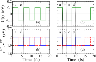
Figure 5: The protocols for the two-stroke pump ((a) and (b)) and the four-stroke pump ((c) and (d)). Shown in plots (a) and (c) are the gate potential $U(t)$ variations, by $0.1\,{\rm eV}$, while plots (b) and (d) shows the time-dependence of the tunnel couplings $v^{\rm LC}=v^{\rm LC}_{01}+v^{\rm LC}_{01}(t)$ (blue lines) and $v^{\rm RC}=v^{\rm RC}_{21}+v^{\rm RC}_{21}(t)$ (red dashed lines), also by $0.1~{}{\rm eV}$. The durations of the strokes are indicated as vertical dashed lines. Values of the other parameters we use are $\varepsilon^{\rm L}=\varepsilon^{\rm R}=\varepsilon^{\rm C}=1\,{\rm eV}$ for the on-site energies, $v^{\rm L}=v^{\rm R}=v_{01}^{\rm LC}=v_{21}^{\rm RC}=2\,{\rm eV}$ for the static tunnel couplings, $\mu_{\rm L}=\mu_{\rm R}=0$ for the chemical potentials of the leads, $E_{f}=0$ for the Fermi energy, and $T_{\rm L}=T_{\rm R}=300\,{\rm K}$ for the temperatures of the leads.

We first study a minimal approach of pumping electrons and energy in our quantum dot device. The time-dependent protocol consists of only two strokes, a and c, as depicted in Fig. 2. In this case, we do not let the electrons charge or discharge via the action of the gate potential. Since only the transport strokes are involved, electrons would flow from the left lead to the channel in stroke a and then proceed to flow to the right lead in stroke c. Following this protocol, the pumped energy would be just enough to move the electrons across the device. The absence of the charging stroke does not allow the electrons to adjust to the higher gate potential within the channel. Thus, the electrons that are transported from the left lead to the channel in stroke a do not get a chance to fully gain energy within the channel, despite the increase in the gate potential. This is because the increase in the gate potential is accompanied by the opening of the transport channel to the right lead. Thus, even though we observe electron pumping in this case, the energy pumped during one cycle is not optimized and hence, there is no extra energy per cycle to be harvested from the pumped electrons.

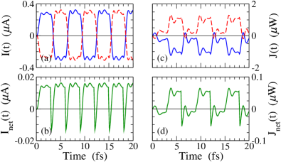
Figure 6: The currents as functions of time for the two-stroke pump. (a) The current from the left lead $I^{\rm L}(t)$ (blue curve) and the current into the right lead $I^{\rm R}(t)$ (red dashed curve). (b) The net current $I_{\rm net}(t)=I^{\rm L}(t)+I^{\rm R}(t)$. (c) The energy current from the left lead $J^{\rm L}(t)$ (blue curve) and the energy current into the right lead $J^{\rm R}(t)$ (red dashed curve). (d) The net energy current $J_{\rm net}(t)=J^{\rm L}(t)+J^{\rm R}(t)$.

Our results are shown in Fig. 6. The gate potential and the lead-channel couplings are varied according to Figs. 5(a) and (b). The stroke durations are $3\,{\rm fs}$ each and the period of pumping cycle is $6\,{\rm fs}$. It is important to stress that even though our time-dependent protocols manipulate the transport through our nonadiabatic pump, the couplings to the leads are always non-zero, implying that electrons may always flow between the leads and the channel. As seen in Fig. 6(a) the electron currents alternate between flowing in and out of the channel. During stroke a, the gate potential lowers the energy level in the channel thus allowing electrons to flow from the left lead to the channel. During stroke c, the gate potential now raises the energy level within the channel, while at the same time the coupling strength to the left lead is decreased, thereby allowing more electrons to flow from the channel to the right lead. In this minimal two-stroke protocol we get a perfect pumping of the electrons, as seen via the net current in Fig. 6(b). The net current is mostly positive indicating a flow of electrons from the left lead to the right with sudden spikes reversing the current flow appearing at the transition points in-between the two strokes. These spikes could be reduced by smoothing out the time-dependent protocol instead of employing abrupt square wave pulses.

The energy current for the two-stroke pump tells a different story, as seen in Figs. 6(c) and (d). The left and right lead currents alternate in the same fashion as the electron current. However, the net energy current flows in the opposite direction to the electron current during stroke a. This implies that even though there are more electrons on average flowing to the right, the electrons flowing to the left have more energy hence reversing the net energy current during stroke a. This makes energy pumping in our two-stroke protocol non-ideal even though during one full cycle the net pumped energy is from left to right. For both electron and energy pumping, the transients last for only one cycle after which the device quickly approaches the periodic asymptotic state. The four-stroke non-adiabatic pump, discussed in Sec. II, overcomes this drawback and causes even the energy current to flow from left to right throughout the cycle, except around sharp transitional points which can be prevented using a smooth protocol instead of an abrupt square wave.

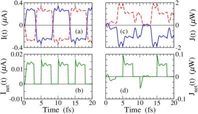
Figure 7: The pumped currents as functions of time for the four-stroke pump. Shown are (a) the electric currents $I^{\rm L}(t)$ (blue curve) and $I^{\rm R}(t)$ (red dashed curve), (b) the net electric current $I_{\rm net}(t)$, (c) the energy currents $J^{\rm L}(t)$ (blue curve) and $J^{\rm R}(t)$ (red dashed curve), and (d) the net energy current $J_{\rm net}(t)$.

In the four-stroke pump, we vary the gate potential and the tunnel couplings according to Figs. 5(c) and (d). The duration of the transport strokes a and c are $3\,{\rm fs}$ while the energy charging and discharging strokes are for $2\,{\rm fs}$. The period of the pumping cycle is $10\,{\rm fs}$ and stroke transitions are sudden and abrupt. The pumped electron and energy currents are shown in Fig. 7. As the pump is being operated, we see from Fig. 7(a) that the left and right currents are alternating between flowing into and out of the channel, similar to the way the currents flow in the two-stroke pump. The net electron current, however, is markedly different from that of the two-stroke pump. Fig. 7(b) shows that the net electron current in each pumping cycle flows to the right. However, during energy charging and discharging strokes we see that the left and right currents exactly cancel, resulting in no net current flow. Similarly, the net energy current shown in Fig. 7(d) shows no net energy current flowing during the energy charging and discharging strokes.

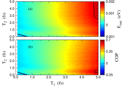
Figure 8: (a) The total output energy $E_{\rm out}$ per cycle and (b) the coefficient of performance ${\rm COP}$ per cycle when the transport stroke durations $T_{1}$ and charging and discharging strokes durations $T_{2}$ are varied. The line at the lower left corner of the plots separates the regions of positive and negative $E_{\rm out}$ and ${\rm COP}$. The dashed line encloses the regions where we obtain the maximum $E_{\rm out}$ and ${\rm COP}$.

The role of the charging and discharging strokes are to increase the energy of the pumped electrons. Longer charging strokes, i.e., larger $T_{2}$, means more pumped energy $E_{\rm out}$ per pumping cycle. In terms of the pump’s performance, however, longer charging strokes do not necessarily lead to better performance. In the ${\rm COP}$ defined in Eq. (9), the input energy $E_{\rm in}$, defined in Eq. (10), also depends on the duration of the strokes. Shown in Fig. 8 are contour plots of the output energy $E_{\rm out}$ and the coefficient of performance ${\rm COP}$ as the durations of the strokes are varied. $T_{1}$ is the duration of transport strokes a and c while $T_{2}$ is the duration of the energy charging stroke b and energy discharging stroke d. Note that there is no data for the $T_{1}=0$ line because we have a non-working pump when the transport strokes are off. Furthermore, the $T_{2}=0$ line indicates data for the two-stroke pump and shows the minimal values for $E_{\rm out}$ and the ${\rm COP}$. Notice that there is a region where both $E_{\rm out}$ and the ${\rm COP}$ are negative, indicating that energy is flowing in the opposite direction and we get a dud energy pump (see the lower left regions below the black lines in Fig. 8). In this regime the stroke durations are too short and the system is continually in the transient regime where rapid oscillations occur after every abrupt stroke transition. The maximum ${\rm COP}$ and $E_{\rm out}$ appear in the region of large transport stroke durations $T_{1}$. Particularly, our pump operates with a relatively large energy output at high coefficient of performance (the regions enclosed by the dashed lines in Fig. 8).

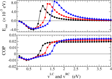
Figure 9: (a)The total output energy per cycle $E_{\rm out}$ and (b) the coefficient of performance per cycle ${\rm COP}$ as functions of the lead-channel couplings $v^{\rm LC}=v^{\rm RC}$. The values of the hopping parameters in the leads are $v^{\rm L}=v^{\rm R}=2\,{\rm eV}$ (circles), $2.5\,{\rm eV}$ (squares), and $3\,{\rm eV}$ (triangles). The on-site energies are maintained at $\varepsilon^{\rm L}=\varepsilon^{\rm R}=1\,{\rm eV}$. The amplitudes of the time-dependent perturbations are $\Delta U=0.01\,{\rm eV}$ and $\Delta v^{\rm LC}=\Delta v^{\rm RC}=0.01\,{\rm eV}$. The durations of the strokes are $T_{1}=2\,{\rm fs}$ and $T_{2}=3\,{\rm fs}$.

We have also investigated the effects of varying the lead-channel coupling on the performance of the pump. Shown in Fig. 9 are the plots of $E_{\rm out}$ and the ${\rm COP}$ when the lead-channel couplings $v^{\rm LC}$ and $v^{\rm RC}$ are varied. In the regions where the couplings are weak, we find that $E_{\rm out}$ and the ${\rm COP}$ are negative indicating a dud energy pump, even though the electron current still flows from the left to the right lead. Transient oscillations after an abrupt stroke transition are large and long-lived when the couplings are weak. For $T_{1}=2\,{\rm fs}$ and $T_{2}=3\,{\rm fs}$, transient oscillations in energy have not dissipated enough resulting in a dud energy pump. As the coupling strengths become stronger, transient oscillations dissipate faster and an output energy that flows from the right to the left lead emerges. Notice that for a given value of $v^{\rm L}$ and $v^{\rm R}$ there is a, possibly resonance, value of around $v^{\rm LC}=v^{\rm L}/2$, and similary for $v^{\rm RC}$, where the $E_{\rm out}$ is maximum. At the strong coupling regions, we find that both $E_{\rm out}$ and the ${\rm COP}$ approach a constant value. Also in this region, higher hopping parameters $v^{\rm L}$ and $v^{\rm R}$ lead to slightly better ${\rm COP}$. This is because higher hopping parameters encourages the electrons to hop from site to site therefore resulting in better transport. In contrast, we have also investigated the effects of varying the on-site energies $\varepsilon^{\rm L}$, $\varepsilon^{\rm R}$, and $\varepsilon^{\rm C}$ as the couplings $v^{\rm LC}$ and $v^{\rm RC}$ are varied. Similar to Fig. 9, the $E_{\rm out}$ and ${\rm COP}$ approach a constant value as the couplings are increased. However, higher on-site energies result in slightly lower performance. This is because higher on-site energies encourages the electrons to stay within the site and is therefore detrimental to transport.

In this work, we have set the temperatures and chemical potentials of the leads to be the same, i.e., $T_{\rm L}=T_{\rm R}=T$ and $\mu_{\rm L}=\mu_{\rm R}=\mu$. The device, therefore, neither has a temperature gradient nor a source-drain bias that can drive currents. The observed currents are due to the synchronized dynamics of the gate potential in the channel and the tunnel couplings between the leads and the channel. We notice, however, that the actual values of $T$ and $\mu$ do affect the amount of output energy $E_{\rm out}$ and the performance ${\rm COP}$ of the pump. Higher temperatures and chemical potentials lead to increased $E_{\rm out}$ and ${\rm COP}$. This can be understood by noting that even though the temperatures and chemical potentials of the leads are the same, the outcome is the net flow of electrons from the left to the right lead. Electrons from a left lead with higher temperature or chemical potential will have more energy thereby resulting in an increase in the total output energy flowing to the right.

V SUMMARY AND CONCLUSION

We model a pump using a nanojunction with time-varying tunnel couplings between the leads and the channel and a dynamic gate potential within the channel. We establish a two-stroke operating protocol and a four-stroke enhanced operating protocol for the pump. At least two transport strokes are needed to pump electrons from the left lead to the right. For the four-stroke pump, the two transport strokes are enhanced by an energy charging stroke and an energy discharging stroke so that the transported electrons gain extra energy when they reach the right lead.

We use nonequilibrium Green’s functions techniques to calculate the electric and energy currents across the device. The technique allows us to establish strong coupling between the leads and the channel and also abrupt, nonadiabatic, changes in the gate potential and the tunnel couplings. A requirement that we employ so that we can arrive at an iterative Dyson equation is that the amplitude of the changes in the gate potential and the tunnel couplings are small compared to typical energy values, such as the on-site energies and the hopping parameters, in the model. Thus, our leads are always connected to the channel making the experimental realization feasible. We also calculate the total energy output to the right lead and the coefficient of performance per cycle of the pump.

Nonequilibrium Green’s functions calculations show both left-moving and right-moving electrons and energy currents toward the left and right leads. The resulting net currents, however, indicate electric currents flowing from the left to the right lead, thereby pumping net electrons in this direction only. In contrast, we see that the dynamics of the energy current does not exactly follow that of the electron current. In instances where the stroke durations are short or the lead-channel couplings are weak, it is possible for the electric current to flow to the right while the energy current flows in the opposite direction. This happens when those electrons that flow to the left have more energy than those that flow to the right, even though there are more right-moving electrons. In the four-stroke pump, the roles of the energy charging and discharging strokes are to enhance the pumped energy and improve the pump’s performance. Longer charging and discharging strokes result in an increase in the output pumped energy. However, longer strokes do not necessarily lead to an improved pump performance due to an accompanying higher input energy required to maintain those strokes.