Anomaly Detection in Beehives using Deep Recurrent Autoencoders

Abstract

Precision beekeeping allows to monitor bees’ living conditions by equipping beehives with sensors. The data recorded by these hives can be analyzed by machine learning models to learn behavioral patterns of or search for unusual events in bee colonies. One typical target is the early detection of bee swarming as apiarists want to avoid this due to economical reasons. Advanced methods should be able to detect any other unusual or abnormal behavior arising from illness of bees or from technical reasons, e.g. sensor failure.
In this position paper we present an autoencoder, a deep learning model, which detects any type of anomaly in data independent of its origin. Our model is able to reveal the same swarms as a simple rule-based swarm detection algorithm but is also triggered by any other anomaly. We evaluated our model on real world data sets that were collected on different hives and with different sensor setups.

1 INTRODUCTION

Precision apiculture, also known as precision beekeeping, aims to support beekeepers in their care decisions to maximize efficiency. For that, sensor data is collected on 1) apiary-level (e.g. meteorological parameters), 2) colony-level (e.g. beehive temperature), or 3) individual bee-related level (e.g. bee counter)  [Zacepins et al., 2015]. To gather data on colony level, beehives are equipped with environmental sensors that continuously monitor and quantify the beehive’s state. Occasionally there are sensor readings that deviate substantially from the norm. We refer to these events as anomalies. They can be categorized as behavior anomalies, sensor anomalies, and external interferences. The first type describes irregular behavior within the monitored subject, the second describes any abnormal measurements of the used sensors, whereas the last can be subsumed as any exterior force operating.

A prominent behavioral anomaly in apiculture is swarming. Swarming is the event of a colony’s queen leaving the hive with a party of worker bees to start a new colony in a distant location. It is a naturally occurring, albeit highly stochastic reproduction process in a beehive. During the prime swarm the current queen departs with many of the workers from the old colony. Subsequent after swarms can occur with fewer workers leaving the hive. Swarming events can reoccur until the total depletion of the original colony [Winston, 1980]. Swarming diminishes a beehive’s production and requires the beekeeper’s immediate attention, if new colonies are to be recollected. Therefore, beekeepers try to prevent swarming events in their beehives.

A second notable behavioral anomaly in beehives are mite infestations (varroa destructor) [Navajas et al., 2008]. They weaken colonies and make bees more susceptible to additional diseases. Over time, they lead to bee deaths and thus have severe consequences to the environment as they reduce the pollination power of bees in general. Just like swarming, mite infestations and diseases require immediate attention by beekeepers.

Sensor anomalies and external interferences are non-bee-related anomalies. They can arise in any sensor network. Any technical defects including faulty sensors can be summarized as sensor anomalies and require maintenance of the beehive and sensor network. In apiaries, external interference is physical interaction of beekeepers, or other external forces, with their hives, e.g. opening the beehive for honey yield.

Finding anomalies in large datasets requires specialized methods that extend beyond manual evaluations. Autoencoders (AEs) are a popular choice in anomaly detection. They are a deep neural network architecture, that is designed to reconstruct normal behavior with minimal loss of information. In contrast, an AE’s reconstruction of anomalous behavior shows significant loss and can therefore be identified. They are purely data-driven without the need for beehive specific knowledge.

In this paper, we present an autoencoder that can detect all three types of anomalies in beehive data in a data-driven fashion. Our contribution is twofold: First, we explore the possibility of using an autoencoder for anomaly detection on beehive data. Second, we show that this architecture can be applied to different types of beehives due to its data-driven origin, without the need for additional fine-tuning.

We evaluate our approach on three datasets: One long term dataset of four years provided by the HOBOS (https://hobos.de/) project, one short term dataset obtained from [Zacepins et al., 2016], and another short term dataset from we4bee (https://we4bee.org/). For this preliminary study, we focus on time spans where swarming can occur to show that our approach is working in general.

The remainder of this paper is structured as follows: Section 2 presents related research. Section 3 describes the used datasets in detail, whereas Section 4 concentrates on a comprehensive characterization of our autoencoder network structure. In Section 5 we describe our experiments and list the results on swarming data in Section 6. Section 7 investigates normal behavior in contrast to selected anomalies, the sensor foundation to detect those with our model, and discusses the results. We conclude with a summary and possible directions for future work in Section 8.

2 RELATED WORK

In order to learn how to distinguish normal from anomalous behavior, we use anomaly detection techniques based on neural networks. In particular, we use recurrent autoencoders, since they have shown to work in many anomaly detection settings with sequential data before [Filonov et al., 2016, Malhotra et al., 2016, Shipmon et al., 2017, Chalapathy and Chawla, 2019]. Prior work for anomaly detection in bee data has focused mainly on swarm detection, for which several techniques have been published.

[Ferrari et al., 2008] monitored sound, temperature and humidity of three beehives to investigate changes of these variables during swarming. The beehives experienced nine swarming activities during the monitoring period, for which they analyzed the collected data. They concluded that the shift in sound frequency and the change in temperature might be used to predict swarming.

[Kridi et al., 2014] proposed an approach to identify pre-swarming behavior by clustering temperatures into typical daily patterns. An anomaly is detected if the measurements do not fit into the typical clusters for multiple hours.

[Zacepins et al., 2016] used a customized swarming detection algorithm based on single-point temperature monitoring. They asserted a base temperature of $34.5\text{\,}\mathrm{\SIUnitSymbolCelsius}$ within the hive, which is allowed to fluctuate within $\pm$ $1\text{\,}\mathrm{\SIUnitSymbolCelsius}$. If an increase of $\geq$ $1\text{\,}\mathrm{\SIUnitSymbolCelsius}$ lasted between two and twenty minutes, they reported the timestamp of the peak temperature as the swarming time.

[Zhu et al., 2019] found, that a linear temperature increase can be observed before swarming. They proposed to measure the temperature between the wall of the hive and the first frame near the bottom which provides the most apparent temperature increase.

While swarming is an important type of anomaly, we believe that other exceptional events should also be detected.

3 DATASETS

We use sensor measurements from HOBOS, a subset of the data from we4bee and the data used by [Zacepins et al., 2016] (referred to as Jelgava) in our work. All datasets are referenced by the location of the beehives.

3.1 Würzburg & Bad Schwartau

HOBOS equipped five beehives (species: apis mellifera; beehive type: zander beehive) with several environmental sensors. We use data from two beehives, located in Bad Schwartau and Würzburg. While there are three verified swarming events at Bad Schwartau, the Würzburg beehive data is completely unlabeled. We use this beehive to assess cross-beehive applicability of our model.

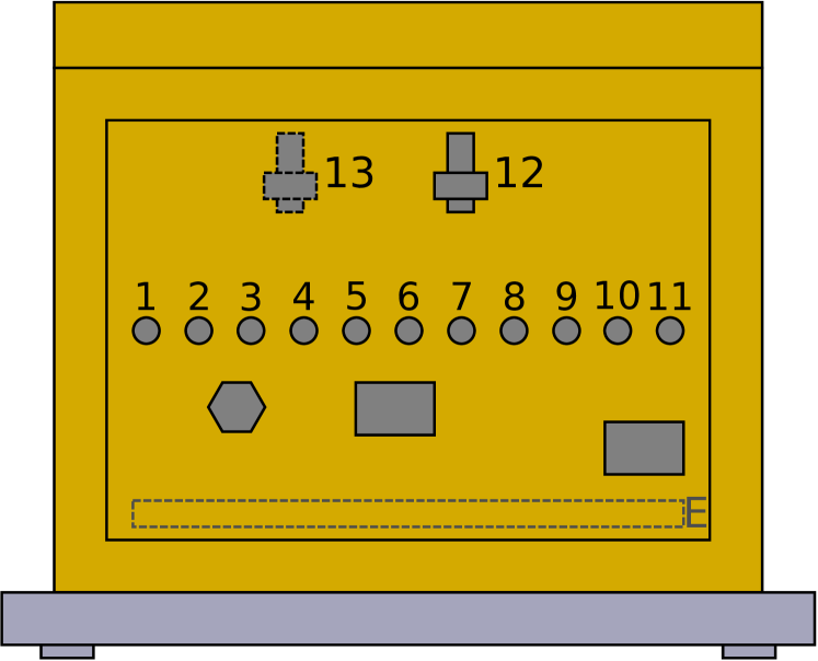
Figure 1: Back of a HOBOS beehive. Temperature sensors T₁–T₁₁ are mounted between honeycombs, temperature sensors T₁₂ and T₁₃ are mounted on the back and the front of the hive, respectively. E denotes the hive’s entrance on the front of the beehive.

Figure 1 shows the back of a HOBOS beehive with all 13 temperature sensors. The beehive in Bad Schwartau is not equipped with T₂, T₃, T₉, T₁₀ and T₁₂ while the one in Würzburg has all sensors except T₂ and T₃. Additionally, weight, humidity and carbon dioxide (CO₂) are measured in the beehives. Measurements are taken once a minute at every sensor. Data was collected from May 2016 through September 2019. As we are mainly interested in swarming events, we only used the data from the typical swarming period May to September of each year for this preliminary study [Fell et al., 1977]. HOBOS granted us access to their complete dataset.

3.2 Jelgava

Ten colonies (apis mellifera mellifera; norwegian-type hive bodies) were monitored by a single temperature sensor placed above the hive body. Measurements were recorded once every minute over the time span of May through August in 2015. The authors granted us access to the nine days in their dataset which contain swarming events, one each day.

3.3 Markt Indersdorf

The colony (apis mellifera; top bar hive) in Markt Indersdorf is monitored by five temperature sensors: one on the outside and four on the inside of the beehive. Three temperature sensors measure laterally to the orientation of the top bars, the remaining one on the inside is placed in parallel at the back. Figure 2 shows a cutaway view of a we4bee hive. Additionally other environmental influences are monitored with sensors for air pressure, weight, fine dust, humidity, rain and wind. Measurements are taken once every second (fine dust: every three minutes). Data ranges from June (start of the colony) through September 2019.

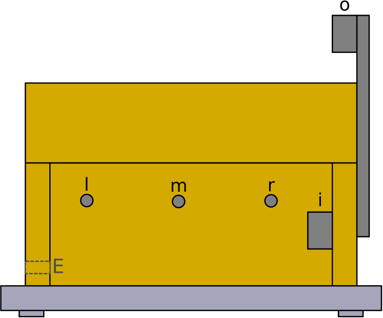
Figure 2: Cutaway view of a we4bee beehive. T_l, T_m, T_r, and T_i are mounted on the inside, laterally to the honeycombs. T_o is placed outside at the pylon. E denotes the entrance on the front of the beehive.

4 AUTOENCODER

Since autoencoders (AE) have proven to be successful for anomaly detection, we use such a model for our task [Goodfellow et al., 2016, Sakurada and Yairi, 2014, Chalapathy and Chawla, 2019]. Especially for analyzing anomalies within sequential data, e.g. time series, deep recurrent autoencoders using long-short-term memory networks (LSTMs) [Goodfellow et al., 2016] have shown great success over conventional methods (e.g. SVM) [Ergen et al., 2017]. We adapt this model for this work.

An autoencoder is a pair of neural networks: an encoder $\phi:\mathcal{X}\rightarrow\mathcal{F}$ and a decoder $\psi:\mathcal{F}\rightarrow\mathcal{X}$, where $\mathcal{X}$ is the input space and $\mathcal{F}$ is the feature space or latent space. In the case of deep recurrent autoencoders, both, encoder and decoder are LSTMs. The training objective of the autoencoder is to reconstruct the input: $\bar{x}=\psi(\phi(x))\sim x$. Usually, the latent space is smaller than the input space, producing a bottleneck that forces the autoencoder to encode patterns of the input data distribution in the encoder’s and decoder’s weights. During the training phase, the autoencoder is provided with data of normal behavior. It learns to reconstruct normal data well. When it encounters abnormal data during inference, i.e. input data that does not fit into the learned patterns, it is not able to reconstruct the input properly. Large deviations between model output and data indicate anomalies.

More formally, the two networks are tuned to minimize a given reconstruction loss function:

$$\phi,\psi=\text{arg min}_{\phi,\psi}\mathcal{L}(x-\psi(\phi(x))).$$

Commonly the $l_{2}$ norm [Zhou and Paffenroth, 2017] or the Mean-Squared-Error (MSE) [Shipmon et al., 2017] are chosen as $\mathcal{L}$. If this loss is greater than a given threshold $\alpha$, the input is considered an anomaly:

$$\mathcal{L}(x-\psi(\phi(x)))=\mathcal{L}(x-\bar{x})\geq\alpha$$

$\alpha$ can be set manually or based on a validation dataset containing anomalies, depending on the desired sensibility of the model. It should ideally be chosen in such a way that all validation anomalies are detected and no normal behavior is misclassified.

5 EXPERIMENTAL SETUP

We evaluate our AE model on beehive data from the four locations described in Section 3.

Data splitting. Both HOBOS hives, Bad Schwartau and Würzburg, were used for training purposes. Through visual analysis of the data, we labeled each day of the dataset as either normal or anomalous. According to [Zacepins et al., 2016, Ferrari et al., 2008] a fully enlarged colony maintains a constant core temperature of $34.5\text{\,}\mathrm{\SIUnitSymbolCelsius}$. All days with much higher or lower temperature readings were considered to contain anomalies. The training and validation set is sampled from the normal portion of the dataset. The holdout set contains all days with abnormal behavior from the beehive used for training, while the test set contains all days with anomalies from any other beehive. Figure 3 visualizes the procedure exemplary when training on the Bad Schwartau hive. Days labeled as abnormal typically also contain fragments of normal behavior. This implies that test and holdout sets are a mixture of normal and anomalous behavior.

Figure 3: The data splits used for Bad Schwartau. The autoencoder is trained on Bad Schwartau’s ‘Training’. The hyperparameters and $\alpha$ are tuned using its ‘Validation’ and ‘Holdout’, respectively. The model is then tested on all ‘Test’. For Würzburg, the splits are set accordingly using its ‘Training’, ‘Validation’, and ‘Test’ as ‘Holdout’. We provide the recording time for all splits.

Input data. We use the centrally located temperature sensor T₆ for the locations Würzburg and Bad Schwartau, in Markt Indersdorf we use T_m, downsampling its measurements to one minute resolution. In Jelgava the only temperature sensor available is utilized. We have also tried T_r for Markt Indersdorf and T₈ for Würzburg and Bad Schwartau in another experiment to analyze differences in predictions when using other sensors.

The temperature data is provided to the model in windows containing a fixed number of subsequent measurements. We used a window size of $60\text{\,}\mathrm{min}$, i.e. 60 measurements, since a swarming event usually ranges from $20\text{\,}\mathrm{min}$ to $60\text{\,}\mathrm{min}$ [Zhu et al., 2019, Zacepins et al., 2016, Ferrari et al., 2008]. For augmentation purposes we built all possible windows of consecutive measurements. All time series were normalized by their z-score.

Model training. We performed a random grid search [Bergstra and Bengio, 2012] to find the best hyperparameters, i.e. the hidden size $hs\in\{2,\ldots,64\}$ and the number of layers $n\in\{1,\ldots,4\}$ for the encoder and decoder LSTMs.

For training we used the Adam optimizer [Kingma and Ba, 2014] with the default parameters (learning rate $10^{-3}$) and MSE as the loss function. To prevent overfitting, we employed early stopping with a patience of five epochs and used a ten percent split of the training data for validation.

As described in Section 4, any time series with a reconstruction error larger than $\alpha$ is considered an anomaly. We selected the threshold manually by examining plots of the found anomalies and gradually decreased this value so that no false positive was detected in the holdout set. As a holdout set we used the test set from the same beehive as the autoencoder was trained on (see Figure 3).

Predictions. The rule-based algorithm described in [Zacepins et al., 2016] (referred to as RBA) was used on all subsets. That is, it was used on the training and testing data from the colonies in Bad Schwartau, Würzburg and Markt Indersdorf, as well as the one in Jelgava itself. We found no swarming events, neither false nor true positives, with this method in any training set, verifying our manual selection of training data. Where possible, we tested it with several temperature sensors.

We trained the AE on both HOBOS hives independently and used their respective holdout set for setting the anomaly threshold. After that, we used this threshold and the trained model as an inference model to predict anomalies in all other anomaly sets, e.g. Bad Schwartau was used to predict anomalies in Würzburg, Jelgava and Markt Indersdorf. Jelgava and Markt Indersdorf were not used for training purposes, since the former only contains anomalous data, and the latter was installed only recently.

6 RESULTS

Table 1 lists all known or found swarming events using the temperature sensor T₆ or T_m.

Table 1: Detected Anomalies. The first column shows the name of the used test (anomaly) set. (S) signifies that the set contains swarms while (O) stands for other anomalies. The next column displays the date of the event, and — where suitable — a reference to subfigures in Figures 4, 6 and 7. The last two columns indicate whether RBA or our method (AE) detected the anomaly. Predictions on HOBOS-hives are based on sensor T₆, on T_m for we4bee. We used the Bad Schwartau trained model to predict the swarms in any other beehive, except for Bad Schwartau itself.

Dataset	Timestamp	Detected
		RBA	AE
Bad Schwartau (S)	2016-05-11 11:054(a)	$\checkmark$	$\checkmark$
	2016-05-22 07:30	$\checkmark$	$\checkmark$
	2017-06-06 15:02	$\checkmark$	$\checkmark$
	2019-05-13 09:30⋆	$\checkmark$	$\checkmark$
	2019-05-21 09:15⋆	$\checkmark$	$\checkmark$
	2019-05-25 12:00⋆	$\checkmark$	$\checkmark$
Bad Schwartau (O)	2016-08-03 17:24	$\checkmark$	$\checkmark$
Würzburg (S)	2019-05-01 09:156(c)		$\checkmark$
	2019-05-10 11:156(b)	$\checkmark$	$\checkmark$
Würzburg (O)	2019-04-17 16:226(a)	$\checkmark$	$\checkmark$
Jelgava (S)	2015-05-06 18:02⋆	$\checkmark$	$\checkmark$
	2016-06-02 13:48⋆	$\checkmark$	$\checkmark$
	2016-05-30 10:03⋆	$\checkmark$	$\checkmark$
	2016-06-16 15:50⋆	$\checkmark$	$\checkmark$
	2016-06-01 13:20⋆	$\checkmark$	$\checkmark$
	2016-06-03 09:11⋆	$\checkmark$	$\checkmark$
	2016-06-13 03:30	$\checkmark$	$\checkmark$
	2016-06-16 10:52⋆	$\checkmark$	$\checkmark$
	2016-06-13 13:32⋆	$\checkmark$	$\checkmark$
Markt Indersdorf (O)	2019-07-26 08:10	$\checkmark$	$\checkmark$
	2019-08-31 17:087(b)	$\checkmark$

This table only lists true positives of swarming events and false positives for comparison. Swarms detected by apiarists on site are marked with ^⋆. Figure 4(a) displays sensor traces of a typical swarming event.

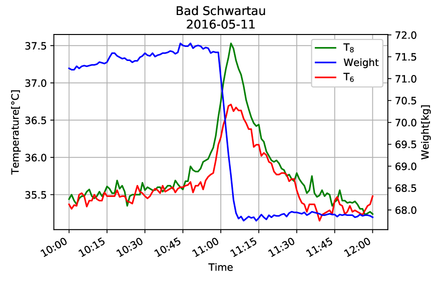
(a) (Prototypical) Swarm as indicated by T₆ and T₈, detected by RBA and AE.

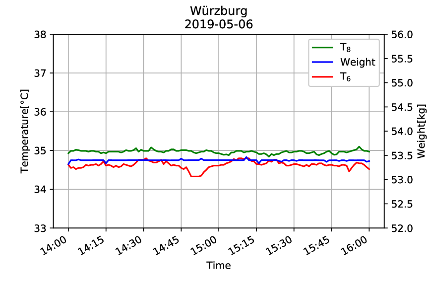
(b) Normal behavior of all three sensors

Figure 4: Exemplary data. (4(a)) Expected variations of all sensors for a swarm. (4(b)) Expected variations of all sensors for normal behavior.

All other swarming events were found by a combination of RBA and our approach: we ran RBA and examined the respective sensor readings to verify a swarming event. Then we applied our AE model to the data and verified that it also found all events detected by RBA. Additionally, we used our approach to find other anomalies or missed swarms.

The table states, that we found all true positives of swarming events, which can be seen in the groups of location (S). Our AE found one additional swarm in Würzburg with T₆ and T₈, which is only found by RBA with T₈. Furthermore, the groups of location (O) list all anomalies detected as swarms by RBA with T₆, but are false positives of swarming events.

Other anomalies are manifold and inherently hard to categorize, such as excited bees due to outside influences, and are thus not included in the table. Three exemplary non-behavioral anomalies are depicted in Figure 7.

7 DISCUSSION

Analysis. Figure 5 displays the inter-sensor correlation using the Pearson correlation coefficient.

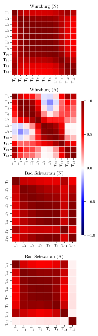
Figure 5: Sensor correlations. All figures display the Pearson correlation between temperature sensors within a given beehive. (N) stands for the dataset containing normal behavior and (A) for the dataset with anomalous behavior.

When observing normal behavior, adjacent sensors correlate highly and positively. Especially the sensors T₄–T₁₀, located centrally inside the hive, show high correlation between each other. Sensors closer to the edges tend to correlate more with outside temperature sensors (T₁₂ and T₁₃). Correlations during the anomalies are weaker, except between neighbors. This confirms the findings in [Zhu et al., 2019], that certain sensor placements tend to capture swarms superiorly.

Figure 6 shows swarm-like anomalies, Figure 7 depicts sensor anomalies and external interferences. All plots contain two temperature sensors (HOBOS: T₆, T₈; we4bee: T_r, T_m), as well as the measured weight. As already mentioned in Section 5, Figure 4(a) shows a prototypical swarm as indicated by all three sensors and detected by both methods.

Figure 6(a) shows an anomaly, that is falsely detected as a swarm when only looking at the temperature sensors. The weight readings show normal behavior, thus contradicting the event trigger initiated by the temperature values.

On the other hand, Figure 6(b) shows a colony swarm, as indicated by all three sensors. If we were to use only one temperature sensor (T₈), both methods would detect three swarms in this window.

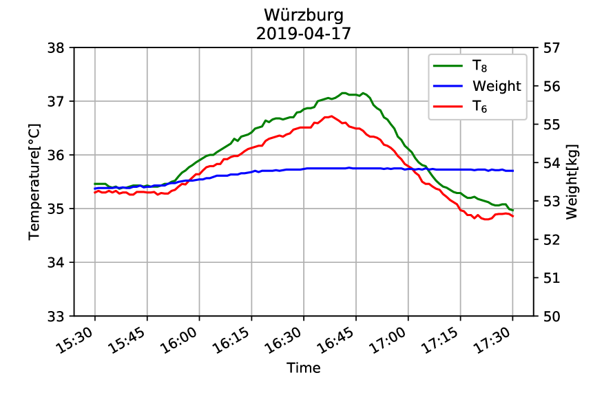
(a) Swarm-like anomaly in sensors T₆ and T₈, but not within the measured weight.

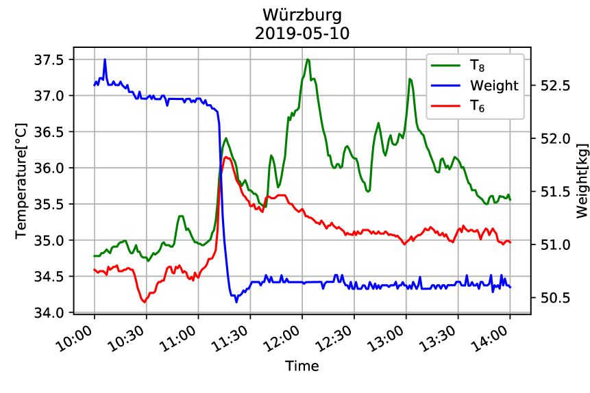
(b) Swarm anomaly indicated by both T₆ and T₈, but additional swarms in T₈. Swarm anomaly within the weight.

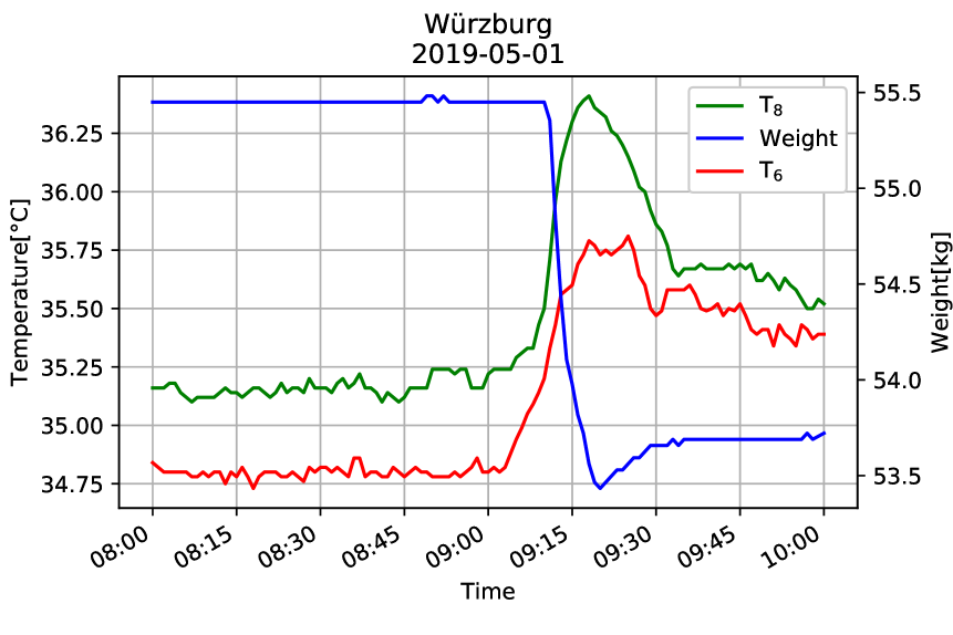
(c) Swarm detected with T₈, but not with T₆ (RBA). Anomaly in both for AE. Swarm anomaly within the weight.

Figure 6: Examples for behavior anomalies of swarm-like events.

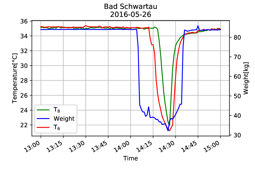
(a) External interference of an opened apiary. The influx of outer air leads to the temperature drop.

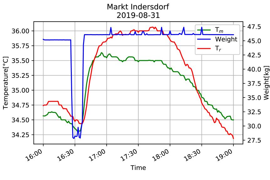
(b) External interference by a possible varroa treatment. The beehive was opened, weight added, leading to the excitement of bees with a temperature increase. In contrast to our AE with T_m, RBA detected a swarm with T_r and T_m.

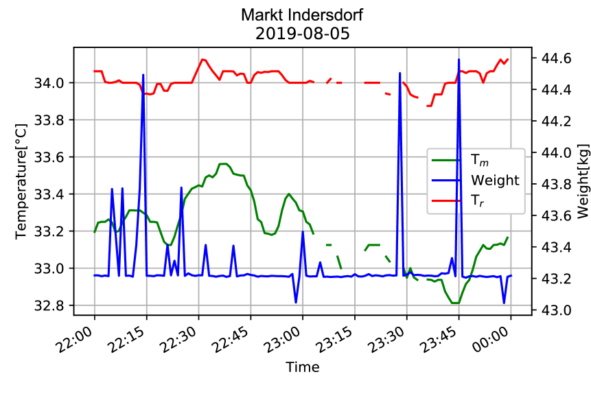
(c) Sensor anomaly with missing values in T_r and T_m, but not in the measured weights.

Figure 7: Examples for external interferences (7(a), 7(b)) and sensor anomalies (7(c)) that are present in the datasets.

In contrast to RBA, AE detects the swarm displayed in Figure 6(c) with temperature sensor T₆. Only with temperature sensor T₈ find this swarm.

Figure 7(a) shows a window in which the beehive was opened, explaining the steep and quick drop in weight. The temperature sensors trail this pattern with different delays, until the hive temperature has cooled to ambient temperature. They quickly return to their initial readings as soon as the hive is closed again.

Figure 7(b) shows a varroa treatment with formic acid (hence the gain in weight). RBA detects swarms in this window for both temperature sensors, whereas our method only detects an anomaly in T_r. That is possibly due to the fact, that sensor readings in T_m are within one standard deviation of the training data.

Table 1 shows only swarm-like anomalies, but our method finds a lot more anomalies. The larger portion of found anomalies are temperature readings well below $30\text{\,}\mathrm{\SIUnitSymbolCelsius}$. Other monitoring anomalies, e.g. Figure 7(a), are detected, too.

Methodology. As described in Section 3, the definition of normal beehavior is vague and the visual division is error prone.

We selected the error threshold $\alpha$ introduced in Section 4 manually, such that no normal behavior is detected as an anomaly in the validation set. This approach allows to control the sensitivity of the AE. It is a trade-off between fine-tuning for swarming detection and suppressing previously unknown anomalies, as seen in Figure 7(b). Methods that determine $\alpha$ automatically also require labeled data.

In Table 1, we listed all known swarms and their respective time of occurrence. Due to the windowing technique described in Section 5, we detect swarms at any position in their respective window. That is, anomalies are detected, both, at the end of the window (predictive estimation) or at the beginning (historical estimation). This prediction quality is highly dependent on the threshold, but enables apiarists to timely react to an ongoing or preeminent swarm.

8 CONCLUSION/FUTURE WORK

In this work we analyzed the possibilities of AEs in a new environment: bee colonies and their habitat. Our model found more swarming events than RBA, a rule based method specifically designed for swarming detection. Additionally, AEs detected not only swarming events but also other anomalies. There are however several aspects with potential for improvements:

Multivariate anomaly detection. HOBOS and we4bee datasets enable us to use multivariate time series in contrast to the presented univariate temperature time series. This allows us to refine predictions even further, as not only an anomaly within sensors is detectable, but an anomaly between sensors, i.e. inter- and intra-sensor anomalies of any type. This could also minimize the overall error if only a subset of sensor shows abnormalities (e.g. in Figure 6(b)).

Method tweaking. Instead of simply using the reconstruction error, we can adapt the loss to make different types of anomalies distinguishable. For example, we could integrate the knowledge of temperature or weight patterns during swarming.

Another possibility to enhance anomaly detection, especially swarming detection, is to include a second training process to introduce $\alpha$ as a trainable parameter. This requires a labeled dataset and is therefore subject to future analysis.

In future work we will experiment with other types of networks, e.g. generative models such as generative adversarial networks or variational autoencoders. This has two key advantages: A) they allow anomalies to be contained in the training set, and B) classification is based on probability rather than reconstruction error [An and Cho, 2015]. The parameter $\alpha$ would then be more interpretable.

Hibernation period. We excluded the months October through March in any dataset (cf. Section 3). Detecting anomalies during this hibernation time is subject to future work, as the assumption of a nearly constant temperature within the colony ($34.5\text{\,}\mathrm{\SIUnitSymbolCelsius}$) is void. Especially in Bad Schwartau, sea wind is an environmental influence that incurs very high deviations from the mentioned normal behavior which also increases the chances of sensor anomalies. Additionally, internal temperature sensors start to mimic the patterns of the outside sensors.

Dataset generation. Due to its data-driven fashion, our method can be improved continuously by integrating collected information in we4bee. This project comprises a broad spatial distribution of apiaries, enabling us to collect a large amount of data fast. Participating apiarists can further improve our model by labeling events presented to them. Furthermore we can use our model as an alert-system to predictively warn beekeepers about ongoing anomalies, whose feedback can again improve our predictions.

References

- An and Cho, 2015 An, J. and Cho, S. (2015). Variational autoencoder based anomaly detection using reconstruction probability. Special Lecture on IE, 2(1).
- Bergstra and Bengio, 2012 Bergstra, J. and Bengio, Y. (2012). Random search for hyper-parameter optimization. JMLR, 13:281–305.
- Chalapathy and Chawla, 2019 Chalapathy, R. and Chawla, S. (2019). Deep learning for anomaly detection: A survey. CoRR, abs/1901.03407.
- Ergen et al., 2017 Ergen, T., Mirza, A. H., and Kozat, S. S. (2017). Unsupervised and semi-supervised anomaly detection with LSTM neural networks. arXiv preprint arXiv:1710.09207.
- Fell et al., 1977 Fell, R. D., Ambrose, J. T., Burgett, D. M., De Jong, D., Morse, R. A., and Seeley, T. D. (1977). The seasonal cycle of swarming in honeybees. Journal of Apicultural Research, 16(4):170–173.
- Ferrari et al., 2008 Ferrari, S., Silva, M., Guarino, M., and Berckmans, D. (2008). Monitoring of swarming sounds in bee hives for early detection of the swarming period. Computers and electronics in agriculture, 64(1):72–77.
- Filonov et al., 2016 Filonov, P., Lavrentyev, A., and Vorontsov, A. (2016). Multivariate industrial time series with cyber-attack simulation: Fault detection using an LSTM-based predictive data model. NIPS Time Series Workshop 2016.
- Goodfellow et al., 2016 Goodfellow, I., Bengio, Y., and Courville, A. (2016). Deep Learning. MIT Press.
- Kingma and Ba, 2014 Kingma, D. P. and Ba, J. (2014). Adam: A method for stochastic optimization. arXiv preprint arXiv:1412.6980.
- Kridi et al., 2014 Kridi, D. S., Carvalho, C. G. N. d., and Gomes, D. G. (2014). A predictive algorithm for mitigate swarming bees through proactive monitoring via wireless sensor networks. In Proceedings of the 11th ACM symposium on PE-WASUN, pages 41–47. ACM.
- Malhotra et al., 2016 Malhotra, P., Tv, V., Ramakrishnan, A., Anand, G., Vig, L., Agarwal, P., and Shroff, G. (2016). Multi-sensor prognostics using an unsupervised health index based on lstm encoder-decoder. 1st SIGKDD Workshop on ML for PHM.
- Navajas et al., 2008 Navajas, M., Migeon, A., Alaux, C., Martin-Magniette, M.-L., Robinson, G., Evans, J. D., Cros-Arteil, S., Crauser, D., and Le Conte, Y. (2008). Differential gene expression of the honey bee apis mellifera associated with varroa destructor infection. BMC genomics, 9(1):301.
- Sakurada and Yairi, 2014 Sakurada, M. and Yairi, T. (2014). Anomaly detection using autoencoders with nonlinear dimensionality reduction. In Proceedings of the MLSDA 2014 2Nd Workshop on Machine Learning for Sensory Data Analysis, MLSDA’14, pages 4:4–4:11. ACM.
- Shipmon et al., 2017 Shipmon, D. T., Gurevitch, J. M., Piselli, P. M., and Edwards, S. T. (2017). Time series anomaly detection; detection of anomalous drops with limited features and sparse examples in noisy highly periodic data. arXiv preprint arXiv:1708.03665.
- Winston, 1980 Winston, M. (1980). Swarming, afterswarming, and reproductive rate of unmanaged honeybee colonies (apis mellifera). Insectes Sociaux, 27(4):391–398.
- Zacepins et al., 2015 Zacepins, A., Brusbardis, V., Meitalovs, J., and Stalidzans, E. (2015). Challenges in the development of precision beekeeping. Biosystems Engineering, 130:60–71.
- Zacepins et al., 2016 Zacepins, A., Kviesis, A., Stalidzans, E., Liepniece, M., and Meitalovs, J. (2016). Remote detection of the swarming of honey bee colonies by single-point temperature monitoring. Biosystems engineering, 148:76–80.
- Zhou and Paffenroth, 2017 Zhou, C. and Paffenroth, R. C. (2017). Anomaly detection with robust deep autoencoders. In Proceedings of the 23rd ACM SIGKDD, pages 665–674. ACM.
- Zhu et al., 2019 Zhu, X., Wen, X., Zhou, S., Xu, X., Zhou, L., and Zhou, B. (2019). The temperature increase at one position in the colony can predict honey bee swarming (apis cerana). Journal of Apicultural Research, 58(4):489–491.