First-Order Methods for Nonconvex Quadratic Minimization

Abstract

We consider minimization of indefinite quadratics with either trust-region (norm) constraints or cubic regularization. Despite the nonconvexity of these problems we prove that, under mild assumptions, gradient descent converges to their global solutions, and give a non-asymptotic rate of convergence for the cubic variant. We also consider Krylov subspace solutions and establish sharp convergence guarantees to the solutions of both trust-region and cubic-regularized problems. Our rates mirror the behavior of these methods on convex quadratics and eigenvector problems, highlighting their scalability. When we use Krylov subspace solutions to approximate the cubic-regularized Newton step, our results recover the strongest known convergence guarantees to approximate second-order stationary points of general smooth nonconvex functions.

1 Introduction

Consider the potentially nonconvex quadratic function

$$f_{A,b}(x)\coloneqq\frac{1}{2}x^{T}Ax+b^{T}x,$$

where $A\in\mathbb{R}^{d\times d}$ is symmetric and possibly indefinite and $b\in\mathbb{R}^{d}$. We wish to solve the problems

$$\mathop{\rm minimize}_{x\in\mathbb{R}^{d}}f_{A,b}(x)~{}\mathop{\rm subject\;to}\left\|{x}\right\|\leq R$$ (P.tr)

and

$$\mathop{\rm minimize}_{x\in\mathbb{R}^{d}}f_{A,b,\rho}(x)\coloneqq f_{A,b}(x)+\frac{\rho}{3}\left\|{x}\right\|^{3},$$ (P.cu)

where $R$ and $\rho\geq 0$ are regularization parameters. These problems arise primarily in the family of trust-region and cubic-regularized Newton methods for general nonlinear optimization [13, 37, 21, 11], which optimize a smooth function $g$ by iteratively minimizing second-order models of $g$ centered at an iterate $x$, which take the form

$$g(y)\approx g_{x}(y)\coloneqq g(x)+\underbrace{\nabla g(x)^{T}(y-x)+\frac{1}{2}(y-x)^{T}\nabla^{2}g(x)(y-x)}_{=f_{\nabla^{2}g(x),\nabla g(x)}(y-x)}.$$

Such models tend to be unreliable when $y$ is far from $x$, particularly in the nonconvex setting when it is possible that $\nabla^{2}g(x)\not\succ 0$. Trust-region and cubic regularization models address this by instead (approximately) iterating

$$y_{k+1}\approx\mathop{\rm argmin}_{\Delta}\left\{f_{\nabla^{2}g(y_{k}),\nabla g(y_{k})}(\Delta)+\mathsf{reg}(\left\|{\Delta}\right\|)\right\},$$ (1)

where $\mathsf{reg}$ regularizes large $\left\|{\Delta}\right\|$; in trust-region methods by a hard constraint so that the model $f_{\nabla^{2}g(y_{k}),\nabla g(y_{k})}$ is accurate, and in cubic-regularization methods by $\left\|{\Delta}\right\|^{3}$ so that the penalized model is a locally accurate upper bound on $g$ [13, 37, 11]. Trust-region and cubic-regularized model-based methods offer a principled and powerful platform for integrating second-order information into the optimization procedure.

The centrality of these methods motivates considerable interest in solving their corresponding subproblems [13, 38, 11, 23, 25, 52]. This becomes computationally challenging in high-dimensional settings, where direct decomposition (or even storage) of the matrix $A$ is infeasible. In many scenarios, however, computing matrix-vector products $v\mapsto Av$ is feasible. As particular examples, when $A$ is sparse or given explicitly by a low-rank factorization, this is feasible; if $A=\nabla^{2}g(x)$ for a smooth function $g$, then $Av=\frac{\nabla g(x+tv)-g(x)}{t}+O(t)$ is approximable to arbitrary accuracy by finite differences; if $A$ is the Hessian of a neural network, we can compute Hessian-vector products efficiently on batches of training data [39, 42] via back-propagation.

1.1 Outline of methods and our contribution

We study first-order methods for solving problems (P.tr) and (P.cu) that access the matrix $A$ only through matrix-vector product evaluations. Our main goal is to characterize the number of evaluations these methods require to reach a desired accuracy $\varepsilon$ in the regime where the problem dimension $d$ is very high. We establish nearly dimension-free bounds—depending at most logarithmically on $d$—highlighting the scalability of first-order methods. In particular, we study gradient descent and Krylov subspace methods, lynchpins of optimization and in frequent use for problems (P.tr) and (P.cu).

Gradient descent

For the trust-region problem (P.tr), gradient descent iterates

$$x_{t+1}=\Pi_{R}(x_{t}-\eta\nabla f_{A,b}(x_{t}))=\Pi_{R}(x_{t}-\eta(Ax_{t}+b)),$$ (2)

where $\eta>0$ is a step size parameter and $\Pi_{R}$ is the Euclidean projection to the ball of radius $R$. For the cubic-regularized problem (P.cu), it is simply

$$x_{t+1}=x_{t}-\eta\nabla f_{A,b,\rho}(x_{t})=(I-\eta A-\rho\eta\left\|{x_{t}}\right\|I)x_{t}-\eta b.$$ (3)

In neither case is $f$ necessarily convex, so it is not a-priori clear that gradient descent even converges to global subproblem solutions; we establish such global convergence under standard and weak assumptions on $\eta$ and the initialization $x_{0}$.

For the cubic regularized problem we prove that the number of steps to reach accuracy $\varepsilon$ scales at most as $\min\{\kappa,\frac{1}{\varepsilon}\}\log\frac{1}{\alpha\varepsilon}$, where $\kappa$ is a problem-dependent condition number and $\alpha=|v_{\min}^{T}b|/\left\|{b}\right\|$ is the normalized inner product between $b$ and the eigenvector of $A$ corresponding to its smallest eigenvalue. We establish these rates by breaking the gradient descent trajectory into two phases and bounding their durations; the first stage consists of the iterate norm rapidly growing away from the origin (thereby escaping all saddle points), while the second stage consists of contraction towards the global solution.

Krylov subspace methods

Krylov subspace methods iterate for $t=1,2,\ldots$ by solving the problems (P.tr) and (P.cu) over the Krylov subspaces

$$\Krylov[t][A,b]\coloneqq\mathrm{span}\{b,Ab,\ldots,A^{t-1}b\}=\{p(A)b\mid\text{$p$ is a degree $t-1$ polynomial}\},$$ (4)

iteratively setting

$$x^{\mathsf{tr}}_{t}=\mathop{\rm argmin}_{x\in\Krylov}\{f_{A,b}(x)\mid\left\|{x}\right\|\leq R\}~{}~{}\mbox{or}~{}~{}x^{\mathsf{cr}}_{t}=\mathop{\rm argmin}_{x\in\Krylov}\{f_{A,b,\rho}(x)\}$$ (5)

for problems (P.tr) and (P.cu), respectively. The Lanczos method can compute these solutions in time dominated by the matrix-vector product cost (see [20, 11, Sec. 2] and Appendix A). Krylov subspace methods are familiar for large-scale numerical problems, including conjugate gradient methods, eigenvector problems, and the solution of linear systems [24, 33, 47, 18].

Since the $t$th iteration of gradient descent (initialized at the origin) lies in $\mathcal{K}_{t}(A,b)$, Krylov subspace methods converge faster than gradient descent by construction. We prove that they are in fact quadratically faster, showing that $\mathcal{K}_{t}(A,b)$ contains an $\varepsilon$-optimal solution in at most $\min\{\sqrt{\kappa}\log\frac{1}{\varepsilon},\frac{1}{\sqrt{\varepsilon}}\log\frac{1}{\alpha}\}$ iterations, with $\kappa$ and $\alpha$ as defined above; this bound applies to both trust-region and cubic-regularized subproblems. Our analysis follows the well-established practice of appealing to uniform polynomial approximations [47, 33] to construct “good” elements in $\mathcal{K}_{t}(A,b)$ achieving the desired convergence. Complementing this approach, we construct additional reference elements in $\mathcal{K}_{t}(A,b)$ based on Nesterov’s accelerated gradient method [35, 36, 49]. The Krylov iterates (5) are then by construction better.

For both gradient descent and Krylov subspace methods, our rates of convergence mirror and unify well-known guarantees for two special cases: convex problems ($A\succeq 0$) and the eigenvector problem ($b=0$ and $A\nsucc 0$) [18, 47]; see Section 7.

Randomization for the “hard case.”

The above iteration count bounds become vacuous for problem instances where $\kappa=\infty$ and $\rho=0$, the “hard case” [13]. We provide two randomization techniques: the first slightly perturbs $b$, and the second expands the Krylov basis (4) in a random direction. These techniques allow us to replace the term $\alpha=|v_{\min}^{T}b|/\left\|{b}\right\|$ with $\frac{1}{\sqrt{d}}$, thus yielding high-probability convergence rates of the form $\frac{1}{\varepsilon}\log\frac{d}{\varepsilon}$ for gradient descent and problem (P.cu), and $\frac{1}{\sqrt{\varepsilon}}\log d$ for Krylov subspace methods for (P.tr) and (P.cu).

A first-order implementation of cubic-regularized Newton steps

Returning to the model-based nonlinear optimization methods motivating our work, we integrate our Krylov subspace solver into a simple version of the cubic-regularized Newton method [21, 37, 50]. Leveraging the analysis of Nesterov and Polyak [37] and our convergence guarantees, we show that for a function $g$ with Lipschitz gradient and Hessian, a method approximating the iteration (1) finds an $\epsilon$ second-order stationary point (satisfying $\left\|{\nabla g(x)}\right\|\leq\epsilon$ and $\lambda_{\min}(\nabla^{2}g(x))\gtrsim-\sqrt{\epsilon}$) with roughly $\epsilon^{-3/2}$ gradient evaluations and $\epsilon^{-7/4}\log\frac{d}{\epsilon}$ Hessian-vector product evaluations. In comparison, simply applying gradient descent on $g$ requires $\epsilon^{-2}$ gradient evaluations to guarantee $\left\|{\nabla g(x)}\right\|\leq\epsilon$ and does not provide a near-positivity guarantee on the Hessian.

1.2 Prior work

Despite their nonconvexity, it is possible to solve the subproblems (P.tr) and (P.cu) to machine precision by iterative solution to linear systems of the form $(A+\lambda I)x=-b$ with Newton-type procedures for the scalar $\lambda$ [13, 11]. To handle large scale instances, earlier work proposes both heuristic variants of the conjugate gradient method [21, 44] and Krylov subspace solutions [20, 11]. While these works demonstrate strong practicality and are in common use, they do not bound the iterations required to obtain approximate solutions. Several works [46, 3, 2] also apply variants of gradient descent to the subproblems (P.tr) and (P.cu) yet without dimension-free convergence guarantees.

A recent thread of research has begun to give (nearly) dimension-free theoretical bounds for first-order-like methods. Hazan and Koren [23] give the first such guarantee, finding an $\varepsilon$-approximate solution with $\widetilde{O}\left({1}/{\sqrt{\varepsilon}}\right)$ matrix-vector products by reducing the trust-region subproblem to a sequence of eigenvector problems and solving them approximately with an efficient first-order method. Ho-Nguyen and Kılınc̨-Karzan [25] provide a different perspective, using a single eigenvector calculation to reformulate the nonconvex quadratic trust-region problem into a convex quadratically constrained quadratic program. Unfortunately, these methods are less conducive to efficient implementation than those above: each has several parameters that require tuning, and we are unaware of numerical experiments testing them.

Zhang et al. [52], in work contemporaneous to the initial submission of the work [6], take an important step towards sharp analysis of practical methods, showing a rate of convergence of the form $\sqrt{\kappa}\log\frac{1}{\varepsilon}$ for Krylov subspace solutions to the trust-region problem. Based on these bounds, the authors propose novel stopping criteria for subproblem solutions in the trust-region optimization method, showing good empirical results. We complete the picture, showing for Krylov subspace methods an $\varepsilon^{-1/2}\log{d}$ convergence guarantee that holds in the hard case where $\kappa=\infty$ and extending the analysis to cubic regularization, for which we also give a comprehensive analysis of gradient descent.

Much of the literature on the problems (P.tr) and (P.cu) considers them in the context of model-based optimization algorithms. Conn et al. [13] provide a detailed account of trust-region methods. Cubic regularization of Newton’s method was first proposed by Griewank [21] and subsequently independently rediscovered by Nesterov and Polyak [37] and Weiser et al. [50]. Nesterov and Polyak [37] prove that for $g$ with Lipschitz Hessian and exact subproblem solutions (1), cubic-regularized Newton’s method finds $\epsilon$ second-order stationary points in order of $\epsilon^{-3/2}$ iterations; this is the first non-asymptotic convergence rate to second-order stationarity as well as the first improvement on gradient descent’s $\epsilon^{-2}$ rate of convergence to first-order stationarity.

Cartis et al. [10] give sufficient conditions on the accuracy of approximate subproblem solutions under which the $\epsilon^{-3/2}$ bound on subproblem number persists, though they leave open how to meet these conditions with a scalable subproblem solver. We provide alternative sufficient conditions, which we satisfy using the Krylov subspace method with roughly $\epsilon^{-1/4}$ Hessian-vector products per subproblem. Our approach is less practical than that of Cartis et al. (assuming knowledge of problem parameters rather than adapting to them as in [11, 10, 13]), but it nevertheless allows us to demonstrate that order roughly $\epsilon^{-7/4}$ gradient and Hessian-vector product evaluations are sufficient to guarantee $\epsilon$ second-order stationarity.

1.3 Concurrent and subsequent work

The papers [6, 5] forming the basis of this paper are part of an active body of research seeking better understanding of and efficient methods for nonconvex optimization. We highlight three lines of work that closely interact with the contributions of our paper.

Improved rates for finding stationary points

Approximate stationarity (a point $x$ satisfying $\left\|{\nabla g(x)}\right\|\leq\epsilon$) serves as a proxy for local optimality, and complexity estimates to achieve it serve as a yardstick for comparing different methods. Gradient descent finds an $\epsilon$-stationary point of functions with Lipschitz gradient in $\epsilon^{-2}$ gradient evaluations [36], and this is unimprovable without further assumptions [9]. Yet additional structure allows improvement: if the Hessian $\nabla^{2}g(x)$ is Lipschitz continuous, several recent first-order methods achieve convergence to $\epsilon$-stationarity in roughly $\epsilon^{-7/4}\log d$ steps. Agarwal et al. [1] propose a variant of the cubic-regularized Newton method with an elaborate subproblem solver based on reduction to eigenvalue computation. In independent work with collaborators Hinder and Sidford [8], we give a different algorithm based on Nesterov’s accelerated gradient descent and the Lanczos method that attains the same first-order complexity. In subsequent work [7] we propose a simpler technique using Nesterov acceleration directly; this method is capable of exploiting even third-order Lipschitz continuity, under which its rate of convergence improves to $\widetilde{O}(\epsilon^{-5/3})$. Royer et al. [40, 41] show that a careful implementation of established techniques (line search and Newton CG) also attains the improved complexity $\widetilde{O}(\epsilon^{-7/4})$. In this paper, we further strengthen this point of view by showing that cubic regularization with a classical Krylov subspace method attains this improved complexity as well.

Large-scale second-order methods

In many large-scale problems—particularly those arising in machine learning—noisy evaluation of the objective and its derivatives is far cheaper than exact evaluation, motivating the use of stochastic gradient methods [4]. Several works attempt to extend second-order model-based optimization techniques to the stochastic setting, with some promising empirical findings [26, 51, 30]. Adopting a theoretical perspective Tripuraneni et al. [48] analyze a sub-sampled cubic-regularized Newton method, solving sub-problems using our gradient descent scheme [6]; the noise inherent in stochastic sampling means that replacing gradient descent with the Krylov subspace method does not improve the leading terms in their complexity bound.

Structured nonconvex problems and their analysis

Global minimization of nonconvex functions is generally intractable [34, 32]. Yet a growing body of work identifies families of practically important structured problems that admit efficient solutions. There are (to us) two broad approaches. The first is a “classical” decoupling approach, which shows that certain local solutions to the problem (e.g., second-order stationary points) are in fact global, and then argues that standard algorithms find these local solutions; examples include matrix completion [16], phase retrieval [45], more general low-rank problems [17], and linear dynamical system identification [22]. The second we term the “dynamics-based” approach, where the trajectory of an optimization method is central and one proves it converges to a global minimum. Here, the simplicity of gradient descent makes it essentially the only feasibly analyzed algorithm, and examples include guarantees for two-layer neural networks [28] and matrix completion, phase retrieval, and blind deconvolution [29]. We view our analysis of gradient descent as a potential prototype for the latter trajectory-based approaches, providing a particularly simple example of the mechanism that keeps gradient descent away from the bad local minimum and allows it to quickly bypass saddle points. In contrast, our analysis of Krylov methods falls firmly in the former approach.

1.4 Paper organization

In Section 2 we define our notation and review basic structural properties of the problems we study. Section 3 gives our results for gradient descent and Section 4 gives our results for Krylov subspace methods. We revisit both methods in Section 5 when we tackle the hard case via randomization. To illustrate our results, we accompany Sections 3–5 with numerical experiments. Then, in Section 6, we apply our randomized Krylov subspace solver within a cubic regularized model-based optimization method for general nonlinear functions, and establish a rate of convergence to approximate second order stationary points. Section 7 concludes our paper by situating our approaches in the context of convergence guarantees for convex optimization and eigenvector problems.

2 Preliminaries and solution structure

Notation

Recall the function $f_{A,b}(x)=\frac{1}{2}x^{T}Ax+b^{T}x$, where $b\in\mathbb{R}^{d}$ and $A\in\mathbb{R}^{d\times d}$ is a symmetric (possibly indefinite) matrix. The eigenvalues of the matrix $A$ are $\lambda^{\left({1}\right)}(A)\leq\cdots\leq\lambda^{\left({d}\right)}(A)$, where the $\lambda^{\left({i}\right)}(A)$ may be negative, and have associated eigenvectors $v_{1},\ldots,v_{d}$, so that $A=\sum_{i=1}^{d}\lambda^{\left({i}\right)}(A)v_{i}v_{i}^{T}$. Importantly, throughout the paper we work in the eigenbasis of $A$, and for any vector $w\in\mathbb{R}^{d}$ we let

$$w^{\left({i}\right)}=v_{i}^{T}w~{}\mbox{denote the $i$th coordinate of $w$ in the eigenbasis of $A$.}$$ (6)

We also let $\lambda_{\min}$ and $\lambda_{\max}$ be the minimum and maximum eigenvalues of $A$, and $v_{\min}$ and $v_{\max}$ be the corresponding (unit) eigenvectors. We let $\left\|{\cdot}\right\|$ be the $\ell_{2}$-operator norm, so $\left\|{A}\right\|=\max_{\left\|{u}\right\|\leq 1}\left\|{Au}\right\|=\max_{i}|\lambda^{\left({i}\right)}(A)|$, and define

$$\beta\coloneqq\left\|{A}\right\|=\max\{-\lambda_{\min},\lambda_{\max}\},$$

Our results frequently depend on the quantity $\beta$, but they hold for any estimate satisfying $\beta\geq\left\|{A}\right\|$. We say a function $g$ is $L$-smooth on a set $X$ if $\left\|{\nabla g(x)-\nabla g(y)}\right\|\leq L\left\|{x-y}\right\|$ for all $x,y\in X$. We denote the positive part of $s\in\mathbb{R}$ by $\left({s}\right)_{+}=\max\{s,0\}$.

2.1 Characterization of solutions

We let ${x_{\star}^{{\mathsf{tr}}}}$ be a solution of the trust region problem (P.tr), while $x_{\star}^{\mathsf{cr}}$ denotes a solution of the cubic-regularized quadratic problem in (P.cu). The structure of the problems allows relatively transparent characterizations of their solutions [e.g. 31, 13, 37]:

Proposition 2.1 ([13], Ch. 7 and [11], Theorem 3.1).

A vector ${x_{\star}^{{\mathsf{tr}}}}$ solves the trust-region problem (P.tr) if and only if there exists $\lambda_{\mathsf{tr}}$ such that

$$(A+\lambda_{\mathsf{tr}}){x_{\star}^{{\mathsf{tr}}}}+b=0,~{}~{}\lambda_{\mathsf{tr}}\geq\left({-\lambda_{\min}}\right)_{+},~{}~{}\mbox{and}~{}~{}\lambda_{\mathsf{tr}}(R-\|{{x_{\star}^{{\mathsf{tr}}}}}\|)=0,$$ (7)

and ${x_{\star}^{{\mathsf{tr}}}}$ is unique if $\lambda_{\mathsf{tr}}>\left({-\lambda_{\min}}\right)_{+}$. A vector $x_{\star}^{\mathsf{cr}}$ solves the cubic-regularized problem (P.cu) if and only if

$$(A+\rho\left\|{x_{\star}^{\mathsf{cr}}}\right\|I)x_{\star}^{\mathsf{cr}}+b=0~{}~{}\mbox{and}~{}~{}\rho\left\|{x_{\star}^{\mathsf{cr}}}\right\|\geq\left({-\lambda_{\min}}\right)_{+},$$ (8)

and $x_{\star}^{\mathsf{cr}}$ is unique if $\rho\left\|{x_{\star}^{\mathsf{cr}}}\right\|>\left({-\lambda_{\min}}\right)_{+}$.

In other words, $x$ solves the corresponding problem if and only if it is stationary and satisfies $\lambda(x)\geq\left({-\lambda_{\min}}\right)_{+}$, where $\lambda(x)$ is the Lagrange multiplier for the constraint $\left\|{x}\right\|\leq R$ for (P.tr) and $\lambda(x)=\rho\left\|{x}\right\|$ for (P.cu); $x$ is unique if $\lambda(x)>\left({-\lambda_{\min}}\right)_{+}$.

For matrices $A$ with distinct eigenvalues, each problem may have a single suboptimal local minimizer, a single local maximizer, and up to $2(d-1)$ saddle points (cf. [21, Section 3] or [31, Thm. 3.1]); see Figure 1 for an example with $d=2$. The next result characterizes the solutions to both the trust-region and cubic-regularized problems in terms of stationarity and the direction $b$ in the space spanned by the eigenvector $v_{\min}$ corresponding to $\lambda_{\min}$. It forms the basis for our analysis of gradient descent.

Proposition 2.2.

Let $b^{\left({1}\right)}\neq 0$. Then ${x_{\star}^{{\mathsf{tr}}}}$ and $x_{\star}^{\mathsf{cr}}$ are the unique stationary points (respectively) of the objectives (P.tr) and (P.cu) satisfying

$$b^{\left({1}\right)}x^{\left({1}\right)}\leq 0~{}~{}~{}\mbox{and so necessarily}~{}~{}~{}b^{\left({1}\right)}x^{\left({1}\right)}<0.$$

Proof.

Let $x$ be a stationary point of either problem and note that it satisfies $Ax+b+\lambda x=0$ for some $\lambda\geq 0$ by Proposition 2.1; for (P.cu) we have $\lambda=\rho\left\|{x}\right\|$ and for (P.tr) $\lambda=\lambda_{\mathsf{tr}}$ is the Lagrange multiplier for the constraint $\left\|{x}\right\|\leq R$. Focusing on the first (eigen)coordinate, we have

$$0=v_{\min}^{T}((A+\lambda I)x+b)=(\lambda_{\min}+\lambda)x^{\left({1}\right)}+b^{\left({1}\right)}.$$

Therefore, $b^{(1)}\neq 0$ implies both $x^{(1)}\neq 0$ and $\lambda+\lambda_{\min}\neq 0$. This strengthens the inequality $b^{(1)}x^{(1)}\leq 0$ to $b^{(1)}x^{(1)}<0$. Hence $\lambda+\lambda_{\min}=-b^{(1)}x^{(1)}/[x^{(1)}]^{2}>0$ and consequently $\lambda>(-\lambda_{\min})_{+}$. By Proposition 2.1 and the above characterization of $\lambda$, the point $x$ is the unique global minimum. ∎

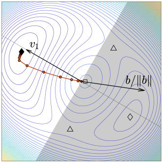
Figure 1: Contour plot of a two-dimensional instance of (P.cu), featuring a local maximum ($\square$), saddle points ($\triangle$), and local minima ($\lozenge$). The line of circles indicates the path of gradient descent initialized at the origin, and the gray area is the half-plane $(v_{1}^{T}b)(v^{T}x)=b^{\left({1}\right)}x^{\left({1}\right)}>0$. Note that the global minimum is the only critical point outside this half-plane (Proposition 2.1). The gradient descent iterates have increasing norm (Lemma 3.1), lie outside the half-plane (Lemma 3.2), and converge to $x_{\star}^{\mathsf{cr}}$ (Proposition 3.1).

2.2 Bounds on the solutions

The magnitude of the solution of (P.cu) and its optimal value are important in our coming analysis (trivially $\left\|{{x_{\star}^{{\mathsf{tr}}}}}\right\|\leq R$), and we therefore provide bounds for these quantities. First, we define

$$A_{\star}\coloneqq A+\rho\left\|{x_{\star}^{\mathsf{cr}}}\right\|I.$$

By Proposition 2.1, $x_{\star}^{\mathsf{cr}}$ solves problem (P.cu) if and only if it is stationary and $A_{\star}\succeq 0$. Let $f(x)=f_{A,b,\rho}(x)=\frac{1}{2}x^{T}Ax+b^{T}x+\frac{\rho}{3}\left\|{x}\right\|^{3}$ for short. Then algebraic manipulation shows that

$$f\left(x\right)=f\left(x_{\star}^{\mathsf{cr}}\right)+\frac{1}{2}(x-x_{\star}^{\mathsf{cr}})^{T}A_{\star}(x-x_{\star}^{\mathsf{cr}})+\frac{\rho}{6}\left(\left\|{x_{\star}^{\mathsf{cr}}}\right\|-\left\|{x}\right\|\right)^{2}\left(\left\|{x_{\star}^{\mathsf{cr}}}\right\|+2\left\|{x}\right\|\right),$$ (9)

which makes it clear that $x_{\star}^{\mathsf{cr}}$ is indeed the global minimum, as both of the $x$-dependent terms are non-negative and minimized at $x=x_{\star}^{\mathsf{cr}}$, and the minimum is unique whenever $\rho\left\|{x_{\star}^{\mathsf{cr}}}\right\|>-\lambda_{\min}$, because $A_{\star}\succ 0$ in this case.

To bound the norm of $x_{\star}^{\mathsf{cr}}$, observe that $\left\|{b}\right\|=\|{A_{\star}x_{\star}^{\mathsf{cr}}}\|\geq(\lambda_{\min}+\rho\left\|{x_{\star}^{\mathsf{cr}}}\right\|)\left\|{x_{\star}^{\mathsf{cr}}}\right\|$. Solving for $\left\|{x_{\star}^{\mathsf{cr}}}\right\|$ gives the upper bound

$$\left\|{x_{\star}^{\mathsf{cr}}}\right\|\leq\frac{-\lambda_{\min}}{2\rho}+\sqrt{\left(\frac{\lambda_{\min}}{2\rho}\right)^{2}+\frac{\left\|{b}\right\|}{\rho}}\leq\frac{\beta}{2\rho}+\sqrt{\left(\frac{\beta}{2\rho}\right)^{2}+\frac{\left\|{b}\right\|}{\rho}}\eqqcolon R_{\rho}$$ (10)

where we recall that $\beta=\left\|{A}\right\|\geq|\lambda_{\min}|$. An analogous lower bound is available:

$$\left\|{x_{\star}^{\mathsf{cr}}}\right\|\geq R_{\mathsf{cr}}\coloneqq\frac{-b^{T}Ab}{2\rho\left\|{b}\right\|^{2}}+\sqrt{\left(\frac{b^{T}Ab}{2\rho\left\|{b}\right\|^{2}}\right)^{2}+\frac{\left\|{b}\right\|}{\rho}}\geq R_{\rho}-\frac{\beta}{\rho}.$$ (11)

The quantity $R_{\mathsf{cr}}$ is the Cauchy radius [13]—the magnitude of the (global) minimizer of $f$ in the span of $b$: $R_{\mathsf{cr}}=\mathop{\rm argmin}_{\zeta\in\mathbb{R}}f(-\zeta b/\|b\|)$. To see the claimed lower bound (11), set $x_{\mathsf{cr}}=-R_{\mathsf{cr}}b/\left\|{b}\right\|$ (the Cauchy point) and note by a calculation that $f(x_{\mathsf{cr}})=-(1/2)\|b\|R_{\mathsf{cr}}-(\rho/6)R_{\mathsf{cr}}^{3}$. Therefore, $0\leq f(x_{\mathsf{cr}})-f(x_{\star}^{\mathsf{cr}})\leq\frac{1}{2}\|b\|(\left\|{x_{\star}^{\mathsf{cr}}}\right\|-R_{\mathsf{cr}})+\frac{1}{6}\rho(\left\|{x_{\star}^{\mathsf{cr}}}\right\|^{3}-R_{\mathsf{cr}}^{3})$, which implies $\left\|{x_{\star}^{\mathsf{cr}}}\right\|\geq R_{\mathsf{cr}}$.

3 Gradient descent for nonconvex quadratics

For the problem of minimizing $f(x)$ subject to constraints that $x\in X$, the projected gradient method begins at $x_{0}\in\mathbb{R}^{d}$ and for a fixed stepsize $\eta>0$ iterates

$$x_{t+1}=\mathop{\rm argmin}_{x\in X}\Big{\{}f(x_{t})+\nabla f(x_{t})^{T}(x-x_{t})+\frac{1}{2\eta}\left\|{x-x_{t}}\right\|^{2}\Big{\}}.$$ (12)

For the trust-region problem (P.tr), where $X=\{x\mid\left\|{x}\right\|\leq R\}$, this is the iteration (2), while for the cubic-regularized problem (P.cu), where $X=\mathbb{R}^{d}$, this is the iteration (3). We will show that the iteration (12) converges to global minimizers for both problems (P.tr) and (P.cu), providing an asymptotic guarantee in Sec. 3.1 and an explicit rate guarantee in Sec. 3.2 for the iteration (3) for problem (P.cu).

Recalling the definitions (10) and (11) of $R_{\rho}$ and $R_{\mathsf{cr}}$ as well as $\left\|{A}\right\|=\beta$, throughout our analysis we make the following assumptions.

Assumption A.

The initialization $x_{0}$ of (12) satisfies $x_{0}=-r\frac{b}{\left\|{b}\right\|}$ where $r\in[0,R]$ for problem (P.tr) or $r\in[0,R_{\mathsf{cr}}]$ for problem (P.cu).

Assumption B.

The step size $\eta$ satisfies $0<\eta\leq\frac{1}{\beta}$ for problem (P.tr) or $0<\eta\leq\frac{1}{4(\beta+\rho R_{\rho})}$ for problem (P.cu).

To select a step size $\eta$ satisfying Assumption B, only a rough upper bound on $\left\|{A}\right\|$ is necessary. One way to obtain such a bound is to apply a few power iterations on $A$.

3.1 Asymptotic convergence guarantees and iterate structure

We begin our analysis via a few properties of the gradient descent trajectory. First, we establish that $\|x_{t}\|$ is monotonic and bounded for the iteration (3) of gradient descent from problem (P.cu).

Lemma 3.1.

Let Assumptions A and B hold. Then the iterates (3) satisfy that $x_{t}^{T}\nabla f_{A,b,\rho}(x_{t})\leq 0$, the norms $\left\|{x_{t}}\right\|$ are non-decreasing with $\left\|{x_{t}}\right\|\leq\left\|{x_{\star}^{\mathsf{cr}}}\right\|$, and $f_{A,b,\rho}$ is $(\beta+2\rho\left\|{x_{\star}^{\mathsf{cr}}}\right\|)$-smooth on the ball $\{x\mid\left\|{x}\right\|\leq\left\|{x_{\star}^{\mathsf{cr}}}\right\|\}$.

This lemma (proved in Appendix B) is the key to our analysis of the cubic-regularized problem. The iterate structure is convenient for both problems, as the next lemma shows that $x_{t}$ and $b$ have opposite signs at all coordinates in the eigenbasis of $A$.

Lemma 3.2.

Let Assumptions A and B hold. Let the iterates $x_{t}$ be generated by the gradient descent iteration (12) for either problem (P.tr) or (P.cu), and let $x_{\star}$ be a solution to the given problem. Then for all $t\geq 0$ and $i\in[d]$,

$$b^{(i)}x_{\star}^{(i)}\leq 0,~{}~{}x_{t}^{(i)}b^{(i)}\leq 0,~{}~{}\text{and}~{}x_{t}^{(i)}x_{\star}^{(i)}\geq 0.$$

Consequently, $x_{\star}^{T}b\leq 0$, and $x_{t}^{T}b\leq 0$ and $x_{t}^{T}x_{\star}\geq 0$ for all $t$.

Proof.

We first show that $b^{\left({i}\right)}x_{\star}^{\left({i}\right)}\leq 0$ for both problems. Letting $\lambda_{\mathsf{tr}}\geq\left({-\lambda_{\min}}\right)_{+}$ be the dual parameter (7), we make the context-dependent definitions $A_{\star}=A+\lambda_{\mathsf{tr}}I$ or $A_{\star}=A+\rho\left\|{x_{\star}^{\mathsf{cr}}}\right\|I$. By Proposition 2.1, we have $A_{\star}x_{\star}=-b$ and $A_{\star}\succeq 0$. Recalling the eigenbasis notation (6), we evidently have $\lambda^{\left({i}\right)}(A_{\star})x_{\star}^{\left({i}\right)}=-b^{\left({i}\right)}$, and therefore $b^{\left({i}\right)}x_{\star}^{\left({i}\right)}=-\lambda^{\left({i}\right)}(A_{\star})[x_{\star}^{\left({i}\right)}]^{2}\leq 0$.

Now, we consider the iterates of gradient descent. The initialization in Assumption A guarantees $x_{0}^{\left({i}\right)}b^{\left({i}\right)}\leq 0$ for either method, forming the base case of our induction. For the trust-region problem, writing the iteration (2) in the eigenbasis gives

$$x_{t+1}^{\left({i}\right)}b^{\left({i}\right)}=\alpha_{t}\left[(1-\eta\lambda^{\left({i}\right)})x_{t+1}^{\left({i}\right)}b^{\left({i}\right)}-\eta[b^{\left({i}\right)}]^{2}\right],~{}~{}~{}\alpha_{t}=\min\left\{1,\tfrac{R}{\left\|{(I-\eta A)x_{t}-\eta b}\right\|}\right\}.$$

As $1-\eta\lambda^{\left({i}\right)}\geq 0$ by Assumption B and $\alpha_{t}>0$, we have that $x_{t}^{\left({i}\right)}b^{\left({i}\right)}\leq 0$ implies $x_{t+1}^{\left({i}\right)}b^{\left({i}\right)}\leq 0$, completing the induction. Writing the cubic-regularized iteration (3) similarly gives

$$x_{t+1}^{\left({i}\right)}b^{\left({i}\right)}=\left(1-\eta\lambda^{(i)}(A)-\eta\rho\|x_{t}\|\right)x_{t}^{(i)}b^{\left({i}\right)}-[b^{\left({i}\right)}]^{2}.$$

Assumption B and Lemma 3.1 imply $1-\eta\lambda^{(i)}(A)-\eta\rho\|x_{t-1}\|\geq 1-\eta(\beta+\rho R_{\rho})>0$ for all $t,i$. Therefore, $x_{t+1}^{(i)}b^{(i)}\leq 0$ by induction.

The remaining claims of the lemma are immediate from the preceding. ∎

Lemmas 3.1, 3.2, and Proposition 2.2 lead to the following guarantee.

Proposition 3.1.

Let Assumptions A and B hold, and assume that $b^{\left({1}\right)}\neq 0$. Let $x_{t}$ follow the gradient iteration (12) for either problem (P.tr) or (P.cu), and $x_{\star}$ solve the corresponding problem. Then $x_{t}\to x_{\star}$ and the objective is monotone decreasing.

Proof.

We recall a few standard results [36, §2.2.3]. For a differentiable $f$, closed convex $X\subset\mathbb{R}^{d}$, and $x\in\mathbb{R}^{d}$, define $\mathsf{T}_{\eta}(x)=\mathop{\rm argmin}_{y\in X}\{\nabla f(x)^{T}(y-x)+\frac{1}{2\eta}\left\|{y-x}\right\|^{2}\}$ and the gradient mapping $\mathsf{G}_{\eta}(x)=\frac{1}{\eta}(x-\mathsf{T}_{\eta}(x))$, where $\mathsf{G}_{\eta}(x)=\nabla f(x)$ if $X=\mathbb{R}^{d}$, so that gradient descent iterates $x_{t+1}=\mathsf{T}_{\eta}(x_{t})$. The first-order optimality conditions for convex optimization give that $(\nabla f(x)-\mathsf{G}_{\eta}(x))^{T}(y-\mathsf{T}_{\eta}(x))\geq 0$ for all $y\in X$, and substituting $y=x$ in this inequality, for any $L$-smooth $f$ we obtain

$$f(\mathsf{T}_{\eta}(x))\leq f(x)-\eta\left(1-\frac{L\eta}{2}\right)\left\|{\mathsf{G}_{\eta}(x)}\right\|^{2}.$$

In the case of problem (P.tr), we have $f(x)=f_{A,b}(x)$ and $L=\beta=\left\|{A}\right\|$, while for (P.cu), $f(x)=f_{A,b}(x)+\frac{\rho}{3}\left\|{x}\right\|^{3}$, which is $L=\beta+2\rho R_{\rho}$-smooth over the ball containing the iterates $x_{t}$ by Lemma 3.1. As $\eta\leq\frac{1}{L}$ for either problem, we have the decrease $f(x_{t+1})\leq f(x_{t})-\frac{\eta}{2}\left\|{\mathsf{G}_{\eta}(x_{t})}\right\|^{2}$, and

$$\frac{\eta}{2}\sum_{\tau=0}^{t-1}\|\mathsf{G}_{\eta}(x_{\tau})\|^{2}\leq f(x_{0})-f(x_{t})\leq f(x_{0})-f(x_{\star}).$$

Let $\hat{x}$ be a limit point of the sequence $x_{t}$, which must satisfy $b^{\left({1}\right)}\hat{x}^{\left({1}\right)}\leq 0$ by Lemma 3.2. The continuity of $x\mapsto\mathsf{G}_{\eta}(x)$ means that $\mathsf{G}_{\eta}(\hat{x})=0$, and consequently $\hat{x}$ is stationary. As $b^{\left({1}\right)}\neq 0$ and $\hat{x}$ is a stationary point with $b^{\left({1}\right)}\hat{x}^{\left({1}\right)}\leq 0$, we have that $\hat{x}=x_{\star}$ by Proposition 2.2. ∎

3.2 Convergence rate guarantees for the cubic-regularized problem

Proposition 3.1 guarantees that gradient descent converges for both problems (P.tr) and (P.cu) whenever $b^{\left({1}\right)}\neq 0$. We now present stronger non-asymptotic guarantees for the cubic problem, deferring the treatment when $b^{\left({1}\right)}=0$ (the so-called “hard case” [13, 11]) to Section 5. (Recall our convention (6), that parenthesized superscripts denote components in the eigenbasis of $A$, and the additional notation $\lambda_{\min}=\lambda^{\left({1}\right)}(A)$ and $\beta=\left\|{A}\right\|$.) We have the following convergence guarantee.

Theorem 3.1.

Let Assumptions A and B hold, $b^{\left({1}\right)}\neq 0$, and $\varepsilon>0$. Define

$$\tau_{\mathrm{grow}}=6\log\left(1+\frac{\left({-\lambda_{\min}}\right)_{+}^{2}}{4\rho|b^{\left({1}\right)}|}\right)~{}\mbox{and}~{}\tau_{\mathrm{converge}}(\varepsilon)=6\log\left(\frac{(\beta+2\rho\left\|{x_{\star}^{\mathsf{cr}}}\right\|)\left\|{x_{\star}^{\mathsf{cr}}}\right\|^{2}}{\varepsilon}\right).$$

Then the gradient descent iterates (3) satisfy $f_{A,b,\rho}(x_{t})\leq f_{A,b,\rho}(x_{\star}^{\mathsf{cr}})+\varepsilon$ for all

$$t\geq\frac{\tau_{\mathrm{grow}}+\tau_{\mathrm{converge}}\left(\varepsilon\right)}{\eta}\min\left\{\frac{1}{\rho\left\|{x_{\star}^{\mathsf{cr}}}\right\|+\lambda_{\min}},\frac{10\left\|{x_{\star}^{\mathsf{cr}}}\right\|^{2}}{\varepsilon}\right\}.$$

Deferring the full proof of the theorem to Appendix C, we provide a brief sketch here. We first show that there is a basin of attraction where iterates with norm above roughly $-\lambda_{\min}/\rho$ contract towards the global solution:

$$\left\|{x_{t+1}-x_{\star}^{\mathsf{cr}}}\right\|^{2}\leq\left[1-\frac{\eta}{6}(\rho\left\|{x_{\star}^{\mathsf{cr}}}\right\|+\lambda_{\min})\right]\left\|{x_{t}-x_{\star}^{\mathsf{cr}}}\right\|^{2}$$ (13)

for all $t$ satisfying

$$\left\|{x_{t}}\right\|\geq r_{\mathrm{thresh}}\coloneqq\frac{-\lambda_{\min}-\frac{1}{3}(\rho\left\|{x_{\star}^{\mathsf{cr}}}\right\|+\lambda_{\min})}{\rho}.$$

As $\left\|{x_{t}}\right\|$ is monotonic by Lemma 3.1, the contraction (13) guarantees that once $\left\|{x_{T_{1}}}\right\|\geq r_{\mathrm{thresh}}$, then $f_{A,b,\rho}(x_{t})-f_{A,b,\rho}(x_{\star}^{\mathsf{cr}})\leq\varepsilon$ for all $t\geq T_{1}+\frac{\tau_{\mathrm{converge}}(\varepsilon)}{\eta}(\rho\left\|{x_{\star}^{\mathsf{cr}}}\right\|+\lambda_{\min})^{-1}$. It remains to establish that the iterates escape the ball of radius $r_{\mathrm{thresh}}$ quickly, which is nontrivial only in the nonconvex setting where $\lambda_{\min}<0$. To this end, we prove the iterate norm grows exponentially, showing that if $\left\|{x_{t}}\right\|\leq r_{\mathrm{thresh}}$ then

$$\left\|{x_{t+1}}\right\|\geq|x^{\left({1}\right)}_{t+1}|\geq\left[1+\frac{\eta}{6}(\rho\left\|{x_{\star}^{\mathsf{cr}}}\right\|+\lambda_{\min})\right]|x^{\left({1}\right)}_{t}|+\eta|b^{\left({1}\right)}|.$$

Consequently, $\left\|{x_{T_{1}}}\right\|\geq r_{\mathrm{thresh}}$ holds for $T_{1}\geq\frac{\tau_{\mathrm{grow}}}{\eta}(\rho\left\|{x_{\star}^{\mathsf{cr}}}\right\|+\lambda_{\min})^{-1}$, establishing the linear convergence rate in Theorem 3.1: the total number of iterations to $\varepsilon$-optimality is $O(\kappa_{\eta}\log\frac{1}{\varepsilon})$, where $\kappa_{\eta}\coloneqq\frac{1}{\eta(\lambda_{\min}+\rho\left\|{x_{\star}^{\mathsf{cr}}}\right\|)}$ has the same order as the problem condition number $\kappa=\frac{\lambda_{\max}+\rho\left\|{x_{\star}^{\mathsf{cr}}}\right\|}{\lambda_{\min}+\rho\left\|{x_{\star}^{\mathsf{cr}}}\right\|}$ when $\eta$ is the maximum step size Assumption B allows and $\lambda_{\max}\geq 0$.

Theorem 3.1 also provides an $O(\frac{1}{\varepsilon}\log\frac{1}{\varepsilon})$ sublinear convergence rate, which is stronger than the linear convergence result when $\lambda_{\min}+\rho\left\|{x_{\star}^{\mathsf{cr}}}\right\|=O(\varepsilon)$. To prove it, we argue that geometric contraction to the optimum still occurs in the subspace of eigenvectors corresponding to eigenvalues greater than $\lambda_{\min}+O(1)\varepsilon/\left\|{x_{\star}^{\mathsf{cr}}}\right\|^{2}$. In the complementary subspace (of eigenvalues close to $\lambda_{\min}$), we argue that the objective $f$ is very smooth outside a ball of radius $r_{\mathrm{thresh}}$, and consequently that errors in that subspace do not significantly affect the objective value.

3.3 Numerical illustration

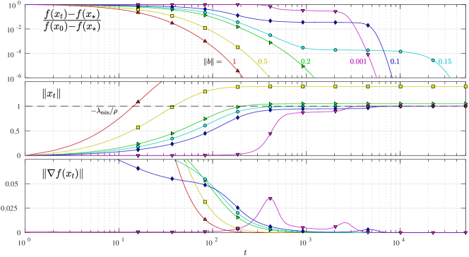
Figure 2: Trajectories of gradient descent with $\lambda^{(1)}(A)=-0.2$ and $\lambda^{(2)}(A),...,\lambda^{(d)}(A)$ equally spaced between $-0.18$ and $\beta=1$, and different vectors $b$ proportional to $[0.01,1,1,1,\ldots]$ in the eigenbasis of $A$. The rest of the parameters are $d=10^{3}$, $\eta=0.1$, $\rho=0.2$ and $x_{0}=0$.

We examine the behavior of gradient descent on a few problem instances, looking at convergence behavior as we vary the vector $b$ by scaling its norm $\left\|{b}\right\|$. The selected norm values $\left\|{b}\right\|\in\{1,0.5,0.2,0.15,0.1,0.001\}$ correspond to condition numbers $(\beta+\rho\left\|{x_{\star}^{\mathsf{cr}}}\right\|)/(\lambda_{\min}+\rho\left\|{x_{\star}^{\mathsf{cr}}}\right\|)\in\{7.6,16,120,5.5\cdot 10^{3},2.9\cdot 10^{4},3.8\cdot 10^{6}\}$; the problem conditioning becomes worse as $\left\|{b}\right\|$ decreases. Figure 2 summarizes our results and describes the settings of the other parameters in the experiment.

The plots show two behaviors of gradient descent. The problem is well-conditioned when $\|b\|\geq 0.2$, and in these cases gradient descent behaves as though the problem were strongly convex, with $x_{t}$ converging linearly to $x_{\star}^{\mathsf{cr}}$. For $\|b\|\leq 0.15$ the problem becomes ill-conditioned and gradient descent stalls around saddle points. Indeed, the third plot of Figure 2 shows that for the ill-conditioned problems, we have $\left\|{\nabla f(x_{t})}\right\|$ increasing over some iterations, which does not occur in convex quadratic problems. The length of the stall does not depend only on the condition number; for $\left\|{b}\right\|=10^{-3}$ the stall is shorter than for $\left\|{b}\right\|\in\{0.1,0.15\}$. Instead, it appears to depend on the norm of the saddle point causing it, which we observe from the value of $\left\|{x_{t}}\right\|$ at the time of the stall; we see that the closer the norm is to $-\lambda_{\min}/\rho$, the longer the stall takes. This is explained by observing that $\nabla^{2}f(x)\succeq(\lambda_{\min}+\rho\left\|{x}\right\|)I$, so every saddle point with norm $\left\|{x}\right\|\approx-\lambda_{\min}/\rho$ must have only small negative curvature and is therefore harder to escape (see also Lemma C.3 in the appendix). Fortunately, as we see in Fig. 2, saddle points with large norm have near-optimal objective value—this is the intuition behind our proof of the sub-linear convergence rates.

4 Krylov subspace methods

We now turn to solutions to (P.tr) and (P.cu) constrained to the Krylov subspaces (4) of order $t$. Given orthogonal $Q_{t}\in\mathbb{R}^{d\times t}$, $Q_{t}^{T}Q_{t}=I$, with columns in $\Krylov$, the subspace-constrained problems (5) reduce to $t$-dimensional updates $y_{t}=\mathop{\rm argmin}_{y:\left\|{y}\right\|\leq R}\{f_{Q_{t}^{T}AQ_{t},Q_{t}^{T}b}(y)\}$ and $y_{t}=\mathop{\rm argmin}_{y}\{f_{Q_{t}^{T}AQ_{t},Q_{t}^{T}b,\rho}(y)\}$ with $x_{t}=Q_{t}y_{t}$. The Lanczos process allows us to compute an orthogonal basis $Q_{t}$ such that $Q_{t}^{T}AQ_{t}$ is tridiagonal in time dominated by the cost of $t$ matrix-vector products. The tridiagonal structure allows fast linear system solution, making the reduced instance solvable in time roughly linear in $t$; see Appendix A for details. Consequently, the computational cost of a Krylov subspace solution of order $t$ is roughly the same as that of $t$ gradient descent steps.

In this section, we develop bounds of the optimality gap of Krylov subspace solution. In contrast to our treatment of gradient descent, here we find it more convenient to obtain guarantees for the trust-region problem, from which we obtain analogous guarantees for the cubic-regularized problem as an immediate corollary.

4.1 Convergence guarantees for the trust region problem

Let

$$x^{\mathsf{tr}}_{t}\in\mathop{\rm argmin}_{x\in\Krylov,~{}\left\|{x}\right\|\leq R}f_{A,b}(x)=\frac{1}{2}x^{T}Ax+b^{T}x$$

denote the order $t$ Krylov subspace solution to the trust region problem (P.tr). With the notation of Section 2 and Proposition 2.1 in particular, our main result on convergence in trust region problems follows.

Theorem 4.1.

For every $t>0$,

$$f_{A,b}(x^{\mathsf{tr}}_{t})-f_{A,b}({x_{\star}^{{\mathsf{tr}}}})\leq 36\left[f_{A,b}(0)-f_{A,b}({x_{\star}^{{\mathsf{tr}}}})\right]\exp\left(-4t\sqrt{\frac{\lambda_{\min}+\lambda_{\mathsf{tr}}}{\lambda_{\max}+\lambda_{\mathsf{tr}}}}\right),$$

and

$$f_{A,b}(x^{\mathsf{tr}}_{t})-f_{A,b}({x_{\star}^{{\mathsf{tr}}}})\leq\frac{(\lambda_{\max}-\lambda_{\min})\left\|{{x_{\star}^{{\mathsf{tr}}}}}\right\|^{2}}{(t-\frac{1}{2})^{2}}\left[4+\frac{\mathbb{I}_{\{\lambda_{\min}<0\}}}{8}\log^{2}\left(\frac{4\left\|{b}\right\|^{2}}{(b^{\left({1}\right)})^{2}}\right)\right].$$

Theorem 4.1 characterizes linear and sublinear convergence regimes. Linear convergence occurs when $t\gtrsim\sqrt{\kappa}$, where $\kappa=\frac{\lambda_{\max}+\lambda_{\mathsf{tr}}}{\lambda_{\min}+\lambda_{\mathsf{tr}}}\geq 1$ is the condition number for the problem, and the error falls beneath $\varepsilon$ in roughly $\sqrt{\kappa}\log{\frac{1}{\varepsilon}}$ Lanczos iterations. Sublinear convergence occurs when $t\lesssim\sqrt{\kappa}$, and there the error decays polynomially and falls beneath $\varepsilon$ in roughly ${1}/{\sqrt{\varepsilon}}$ iterations. For worst-case problem instances this characterization is tight to numerical constant factors [5, Sec. 4].

The guarantees of Theorem 4.1 closely resemble the guarantees for the conjugate gradient method [47], including them as the special case $R=\infty$ and $\lambda_{\min}\geq 0$. For convex problems, the radius constraint $\left\|{x}\right\|\leq R$ always improves the conditioning of the problem, as $\frac{\lambda_{\max}}{\lambda_{\min}}\geq\frac{\lambda_{\max}+\lambda_{\mathsf{tr}}}{\lambda_{\min}+\lambda_{\mathsf{tr}}}$; the smaller $R$ is, the better conditioned the problem becomes; see additional discussion in Sec. 7. For nonconvex problems, the sublinear rate features an additional logarithmic term that captures the role of the eigenvector $v_{\min}$. The first rate of Theorem 4.1 is similar to those of Zhang et al. [52, Thm. 4.11], though with somewhat more explicit dependence on $t$.

In the “hard case,” which corresponds to $b^{\left({1}\right)}=0$ and $\lambda_{\min}+\lambda_{\mathsf{tr}}=0$ (cf. [13, Ch. 7]), both the bounds in Theorem 4.1 become vacuous, and indeed $x^{\mathsf{tr}}_{t}$ may not converge to the global minimizer in this case. However, as the sublinear bound of Theorem 4.1 depends only logarithmically on $b^{\left({1}\right)}$, it remains valid even extremely close to the hard case. In Section 5 we describe simple randomization techniques with convergence guarantees that are valid in the hard case as well.

For convenience of the reader, we provide a sketch of the proof of Theorem 4.1 here, deferring the full proof to Appendix D. Our analysis rests on two elementary observations. First Krylov subspaces are invariant to shifts by scaled identity matrices, i.e. $\mathcal{K}_{t}(A,b)=\mathcal{K}_{t}(A_{\lambda},b)$ for any $A,b,t$ where $\lambda\in\mathbb{R}$, and

$$A_{\lambda}\coloneqq A+\lambda I.$$

Second, for every point $x$ and $\lambda\in\mathbb{R}$

$$f_{A,b}(x)-f_{A,b}({x_{\star}^{{\mathsf{tr}}}}) =f_{A_{\lambda},b}(x)-f_{A_{\lambda},b}({x_{\star}^{{\mathsf{tr}}}})+\frac{\lambda}{2}(\left\|{{x_{\star}^{{\mathsf{tr}}}}}\right\|^{2}-\left\|{x}\right\|^{2})$$ (14)

Our strategy then is to choose $\lambda$ such that $A_{\lambda}\succeq 0$, and then use known results to find $y_{t}\in\Krylov[t][A_{\lambda},b]=\Krylov[t][A,b]$ that rapidly reduces the “convex error” term $f_{A_{\lambda},b}(y_{t})-f_{A_{\lambda},b}({x_{\star}^{{\mathsf{tr}}}})$. We then adjust $y_{t}$ to obtain a feasible point $x_{t}$ such that the “norm error” term $\frac{\lambda}{2}(\left\|{{x_{\star}^{{\mathsf{tr}}}}}\right\|^{2}-\left\|{x_{t}}\right\|^{2})$ is small. To establish linear convergence, we take $\lambda=\lambda_{\mathsf{tr}}$ and adjust the norm of $y_{t}$ by taking $x_{t}=(1-\alpha)y_{t}$ for some small $\alpha$ that guarantees $x_{t}$ is feasible and that the “norm error” term is small. To establish sublinear convergence we set $\lambda=-\lambda_{\min}$ and take $x_{t}=y_{t}+\alpha\cdot z_{t}$, where $z_{t}$ is an approximation for $v_{\min}$ within $\Krylov$, and $\alpha$ is chosen to make $\left\|{x_{t}}\right\|=\left\|{{x_{\star}^{{\mathsf{tr}}}}}\right\|$. This means the “norm error” vanishes, while the “convex error” cannot increase too much, as $A_{-\lambda_{\min}}z_{t}\approx A_{-\lambda_{\min}}v_{\min}=0$.

4.2 Convergence guarantees for the cubic-regularized problem

Comparing the optimality characterization (8) for the cubic problem (P.cu) to that for the trust-region problem (7), we see that any instance $(A,b,\rho)$ of cubic regularization has an equivalent trust-region instance $(A,b,R)$, with $R=\left\|{x_{\star}^{\mathsf{cr}}}\right\|$ and identical global minimizers. This trust-region instance has optimal Lagrange multiplier $\lambda_{\mathsf{tr}}=\rho\left\|{x_{\star}^{\mathsf{cr}}}\right\|$, and at any trust-region feasible $x$ (satisfying $\left\|{x}\right\|\leq R=\left\|{x_{\star}^{\mathsf{cr}}}\right\|=\left\|{{x_{\star}^{{\mathsf{tr}}}}}\right\|$), the cubic-regularization optimality gap is smaller than its trust-region equivalent,

$$f_{A,b,\rho}(x)-f_{A,b,\rho}(x_{\star}^{\mathsf{cr}})=f_{A,b}(x)-f_{A,b}({x_{\star}^{{\mathsf{tr}}}})+\frac{\rho}{3}\big{(}\left\|{x}\right\|^{3}-\|{{x_{\star}^{{\mathsf{tr}}}}}\|^{3}\big{)}\leq f_{A,b}(x)-f_{A,b}({x_{\star}^{{\mathsf{tr}}}}).$$

Letting $x^{\mathsf{cr}}_{t}$ denote the minimizer of $f_{A,b,\rho}$ in $\Krylov$ and letting $x^{\mathsf{tr}}_{t}$ denote the Krylov subspace solution of the equivalent trust-region problem, we conclude that

$$f_{A,b,\rho}(x^{\mathsf{cr}}_{t})-f_{A,b,\rho}(x_{\star}^{\mathsf{cr}})\leq f_{A,b,\rho}(x^{\mathsf{tr}}_{t})-f_{A,b,\rho}(x_{\star}^{\mathsf{cr}})\leq f_{A,b}(x^{\mathsf{tr}}_{t})-f_{A,b}({x_{\star}^{{\mathsf{tr}}}});$$

cubic regularization Krylov subspace solutions always have a smaller optimality gap than their trust-region equivalents. Theorem 4.1 thus gives the following result.

Corollary 4.2.

Let $f_{A,b,\rho}^{\star}=f_{A,b,\rho}(x_{\star}^{\mathsf{cr}})$. For every $t>0$,

$$f_{A,b,\rho}(x^{\mathsf{cr}}_{t})-f_{A,b,\rho}^{\star}\leq 36\left[f_{A,b,\rho}(0)-f_{A,b,\rho}^{\star}\right]\exp\left\{-4t\sqrt{\frac{\lambda_{\min}+\rho\left\|{x_{\star}^{\mathsf{cr}}}\right\|}{\lambda_{\max}+\rho\left\|{x_{\star}^{\mathsf{cr}}}\right\|}}\right\},$$

and

$$f_{A,b,\rho}(x^{\mathsf{cr}}_{t})-f_{A,b,\rho}^{\star}\leq\frac{(\lambda_{\max}-\lambda_{\min})\left\|{x_{\star}^{\mathsf{cr}}}\right\|^{2}}{(t-\frac{1}{2})^{2}}\left[4+\frac{\mathbb{I}_{\{\lambda_{\min}<0\}}}{8}\log^{2}\left(\frac{4\left\|{b}\right\|^{2}}{(b^{\left({1}\right)})^{2}}\right)\right].$$

Proof.

We look forward to use the bound (39) in the proof of Theorem 4.1 (Appendix D) with the inequality $18({x_{\star}^{{\mathsf{tr}}}})^{T}A_{\lambda_{\mathsf{tr}}}{x_{\star}^{{\mathsf{tr}}}}+4\lambda_{\mathsf{tr}}\left\|{{x_{\star}^{{\mathsf{tr}}}}}\right\|^{2}\leq 36[\frac{1}{2}{x_{\star}^{\mathsf{cr}}}^{T}Ax_{\star}^{\mathsf{cr}}+\frac{1}{6}\rho\left\|{x_{\star}^{\mathsf{cr}}}\right\|^{3}]=36[f_{A,b,\rho}(0)-f_{A,b,\rho}(x_{\star}^{\mathsf{cr}})]$. ∎

4.3 Numerical illustration

To illustrate our convergence rate guarantees, for each of three controlled condition numbers $\kappa=\frac{\lambda_{\max}+\rho\left\|{x_{\star}^{\mathsf{cr}}}\right\|}{\lambda_{\min}+\rho\left\|{x_{\star}^{\mathsf{cr}}}\right\|}\in\{10^{2},10^{4},10^{6}\}$, we generate 5,000 random cubic-regularization problems $f=f_{A,b,\rho}$ in dimension $d=10^{6}$ (see Appendix F for more details). We solve these problems with both gradient descent (with step size $\eta=\frac{1}{4}$) and the Krylov subspace method. Figure 3 summarizes the result, showing the cumulative distribution (represented by shading) of suboptimality $\frac{f(x_{t})-f(x_{\star}^{\mathsf{cr}})}{f(0)-f(x_{\star}^{\mathsf{cr}})}$ versus iteration number across the generated instances.

As the figure shows, about 20 Lanczos iterations suffice to solve even the worst-conditioned instances to about $10\%$ relative accuracy, and 100 iterations give accuracy better than $1\%$. Moreover, for $t\gtrapprox\sqrt{\kappa}$, the approximation error decays exponentially with precisely the rate $4/\sqrt{\kappa}$ predicted by our analysis, for almost all the generated problems. For $t\ll\sqrt{\kappa}$, the error decays approximately as $t^{-2}$. Gradient descent converges more slowly, exhibiting linear convergence for low $\kappa$ and sublinear convergence with rate $1/t$ when $\kappa$ is large. This is consistent with our bounds from Section 3.2.

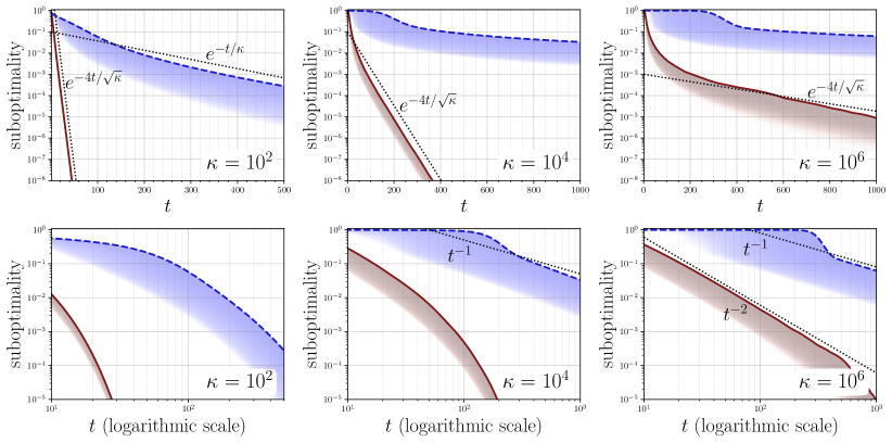
Figure 3: Optimality gap of Krylov subspace solutions (red, solid line) and gradient descent (blue, dashed line) on random cubic-regularization problems, versus iteration count $t$. The shaded regions indicate the cumulative distribution of the optimality gap as a function of $t$, and the bold lines show the maximum value across all generated problems. Columns correspond to different condition numbers $\kappa=({\lambda_{\max}+\rho\left\|{x_{\star}^{\mathsf{cr}}}\right\|})/({\lambda_{\min}+\rho\left\|{x_{\star}^{\mathsf{cr}}}\right\|})$, and rows differ by scaling of the $t$ axis (linear at the top and logarithmic at the bottom).

5 Randomizing away the hard case

Both gradient descent and Krylov subspace methods may fail to converge to the global solution of problems (P.tr) and (P.cu) in the “hard case” [13, 38], that is, when $b^{\left({1}\right)}=v_{\min}^{T}b=0$. This is unavoidable, since in this case methods generate iterates in a subspace orthogonal to $v_{\min}$, while $x_{\star}^{\left({1}\right)}$ may be non-zero. Yet as with eigenvector methods [27, 18], simple randomization approaches address the hard case with high probability, at the cost of introducing a logarithmic dependence on $d$ to the error bounds. We describe two approaches: one that perturbs the data $b$, and one that expands the span of the iterates.

5.1 Data perturbation

Our first approach is to perturb $b$ to a random vector $\tilde{b}$ very near $b$, which guarantees that $\tilde{b}^{\left({1}\right)}\neq 0$, while being near enough $b$ that the corresponding perturbed solutions nearly solve the initial problem. We showcase this approach for gradient descent on the cubic regularized problem; analogous results for Krylov subspace methods for both trust region and cubic regularization are straightforward [5, Cor. 3].

Corollary 5.1.

Let Assumptions A and B hold, let $\varepsilon,\delta>0$, and let $u\sim\mathsf{Uni}(\mathbb{S}^{d-1})$. Let $\tilde{x}_{t}$ be generated by the gradient descent iteration (3) for problem (P.cu) with $\tilde{b}=b+\sigma u$ replacing $b$, where

$$\sigma=\frac{\rho\varepsilon}{\beta+2\rho\left\|{x_{\star}^{\mathsf{cr}}}\right\|}\cdot\frac{\overline{\sigma}}{12}~{}\mbox{with}~{}\overline{\sigma}\leq 1.$$

Then with probability at least $1-\delta$, we have $f_{A,b,\rho}(\tilde{x}_{t})\leq f_{A,b,\rho}(x_{\star}^{\mathsf{cr}})+(1+\overline{\sigma})\varepsilon$ for

$$t\geq\frac{6\tilde{\tau}_{\mathrm{grow}}(\delta,\overline{\sigma})+14\tilde{\tau}_{\mathrm{converge}}\left(\varepsilon\right)}{(1+\overline{\sigma})^{-1}\eta}\min\left\{\frac{1}{\lambda_{\min}+\rho\left\|{x_{\star}^{\mathsf{cr}}}\right\|},\frac{10\left\|{x_{\star}^{\mathsf{cr}}}\right\|^{2}}{\varepsilon}\right\}.$$

where $\tilde{\tau}_{\mathrm{grow}}(\delta,\overline{\sigma})\coloneqq\log\Big{(}1+\frac{3\mathbb{I}_{\{\lambda_{\min}<0\}}\sqrt{d}}{\overline{\sigma}\delta}\Big{)}$ and $\tilde{\tau}_{\mathrm{converge}}(\varepsilon)\coloneqq\log\left(\frac{(\beta+2\rho\left\|{x_{\star}^{\mathsf{cr}}}\right\|)\left\|{x_{\star}^{\mathsf{cr}}}\right\|^{2}}{\varepsilon}\right)$.

See Appendix E.1 for a proof.

5.2 Subspace perturbation for Krylov methods

For Krylov subspace methods we need not perturb the data and may instead draw a spherically symmetric random vector $u$ and use the joint Krylov subspace

$$\Krylov[t][A,\{b,u\}]\coloneqq\mathrm{span}\{b,Ab,\ldots,A^{t-1}b,u,Au,\ldots,A^{t-1}u\}.$$

The block Lanczos method [14, 19] efficiently solves both the trust-region and cubic-regularized problems over $\Krylov[t][A,\{b,u\}]$, iterating

$$\hat{x}^{\mathsf{tr}}_{t}\in\mathop{\rm argmin}_{x\in\Krylov[t][A,\{b,u\}],\left\|{x}\right\|\leq R}f_{A,b}(x)~{}~{}~{}\mbox{and}~{}~{}\hat{x}^{\mathsf{cr}}_{t}\in\mathop{\rm argmin}_{x\in\Krylov[t][A,\{b,u\}]}f_{A,b,\rho}(x)$$

for $u\sim\mathsf{Uni}(\mathbb{S}^{d-1})$; we review the technique in Appendix A.1. Theorem 4.1 and Corollary 4.2 then nearly immediately imply the following convergence guarantee, whose proof we provide in Appendix E.3.

Corollary 5.2.

Let $0<\delta<1$ and $\hat{x}^{\mathsf{tr}}_{t}$ and $\hat{x}^{\mathsf{cr}}_{t}$ be as above, where $u\sim\mathsf{Uni}(\mathbb{S}^{d-1})$. With probability at least $1-\delta$ over the choice of $u$, for all $t\in\mathbb{N}$

$$f_{A,b}(\hat{x}^{\mathsf{tr}}_{t})-f_{A,b}({x_{\star}^{{\mathsf{tr}}}})\leq\frac{(\lambda_{\max}-\lambda_{\min})R^{2}}{t^{2}}\left[4+\frac{\mathbb{I}_{\{\lambda_{\min}<0\}}}{2}\log^{2}\left(\frac{4d}{\delta^{2}}\right)\right]$$

and

$$f_{A,b,\rho}(\hat{x}^{\mathsf{cr}}_{t})-f_{A,b,\rho}(x_{\star}^{\mathsf{cr}})\leq\frac{(\lambda_{\max}-\lambda_{\min})\left\|{x_{\star}^{\mathsf{cr}}}\right\|^{2}}{t^{2}}\left[4+\frac{\mathbb{I}_{\{\lambda_{\min}<0\}}}{2}\log^{2}\left(\frac{4d}{\delta^{2}}\right)\right].$$

Corollary 5.2 implies we can solve the trust-region problem to $\epsilon$ accuracy in roughly $\epsilon^{-1/2}\log d$ matrix-vector products, even in the hard case. The main drawback of this randomization approach is that half the matrix-vector products are expended on the random vector; when the problem is well-conditioned or when $|b^{\left({1}\right)}|/\|{b}\|$ is not extremely small, using the standard subspace solution is nearly twice as fast. In comparison to the data perturbation strategy (Corollary 5.1), however, the subspace perturbation strategy converges to the optimal solutions with probability 1 rather than hitting an error floor due to the choice of perturbation magnitude $\sigma$.

5.3 Numerical illustration

To test the effect of randomization, we generate “hard case” problem instances (with $\kappa=\infty$; see details in Appendix F) and compare the subspace randomization scheme (Section 5.2) with data perturbation (Section 5.1) applied to a Krylov subspace solver with different magnitudes of the perturbation parameter $\sigma$. Figure 4 shows the results: for any fixed target accuracy, some choices of $\sigma$ yield faster convergence than the joint subspace scheme. However, for any fixed $\sigma$, optimization eventually hits a noise floor, while the joint subspace scheme continues to improve. Choosing $\sigma$ requires striking a balance: if too large, the noise floor is high and may be worse than no perturbation at all; if too small, escaping the unperturbed error level will take too long, and the method might falsely declare convergence. A practical heuristic for safely choosing $\sigma$ is an interesting topic for future research.

Figure 4: Optimality gap of Krylov subspace solutions on random cubic-regularization problems, versus matrix-vector product number $t$. Each line represents median suboptimality, and shaded regions represent inter-quartile range. Different lines correspond to different randomization settings.

6 A Hessian-free majorization method

As the final component of our development, we use our results to analyze the optimization scheme (1), where we use the Krylov solver (5) to approximate cubic-regularized Newton steps. Our purpose is to demonstrate that a method close to practically effective nonlinear optimization methods—such as trust-region [13] or Adaptive Regularization of Cubics (ARC) [11]—achieves convergence guarantees dominating those possible for gradient descent.

We wish to minimize a twice differentiable function $g:\mathbb{R}^{d}\to\mathbb{R}$. More precisely, we assume that the Hessian $\nabla^{2}g$ of $g$ is $\rho$-Lipschitz continuous, and we follow Nesterov and Polyak [37] (see also [11, 15]) to seek an $\epsilon$-second-order stationary point $y_{\epsilon}$:

$$\left\|{\nabla g(y_{\epsilon})}\right\|\leq\epsilon~{}~{}\textrm{and}~{}~{}\nabla^{2}g(y_{\epsilon})\succeq-\sqrt{\rho\epsilon}I.$$ (15)

Such points approximately satisfy second-order necessary conditions for local minima, providing a stronger guarantee than $\epsilon$-stationary points satisfying only $\left\|{\nabla g(y)}\right\|\leq\epsilon$.

We revisit method (1), which iteratively minimizes regularized quadratic models of the function $g$. To guarantee convergence, we impose a few assumptions on $g$.

Assumption C.

The function $g$ satisfies $\inf g=g_{\star}>-\infty$, is $\beta$-smooth and has $2\rho$-Lipschitz Hessian, i.e., $\left\|{\nabla^{2}g(y)-\nabla^{2}g(y^{\prime})}\right\|\leq 2\rho\left\|{y-y^{\prime}}\right\|$ for all $y,y^{\prime}\in\mathbb{R}^{d}$.

The assumptions on boundedness and smoothness are standard, while the third implies [37, Lemma 1] that a cubic-regularized quadratic model bounds $g$: for all $x,y$,

$$g(x)\leq g(y)+\nabla g(y)^{T}(x-y)+\frac{1}{2}(x-y)^{T}\nabla^{2}g(y)(x-y)+\frac{\rho}{3}\left\|{x-y}\right\|^{3}.$$ (16)

For simplicity we assume that the constants $\beta$ and $\rho$ are known. This is benign, as we may estimate these constants without significantly affecting the complexity bounds, though in practice, careful adaptive estimation of $\rho$ is crucial for good performance, a primary strength of the ARC method [11].

Algorithm 1 A second-order majorization method

1:function Find-SOSP($y_{0}$, $g$, $\beta$, $\rho$, $\epsilon$, $\delta$)

2:     Set $r=\sqrt{\frac{\epsilon}{9\rho}}$

3:     for $k=1,2,\ldots$ do $\triangleright$ guaranteed to terminate in at most $O(\epsilon^{-3/2})$ iterations

4:         $\Delta_{k}\leftarrow\hyperref@@ii[func:SSP]{\textsc{Solve-CR}(\nabla^{2}g(y_{k-1}),\ \nabla g(y_{k-1}),\ \rho,\ \beta,\ r,\ \frac{\delta}{2k^{2}})}$

5:         $y_{k}\leftarrow y_{k-1}+\Delta_{k}$

6:         if  $g(y_{k})>g(y_{k-1})-\frac{1}{12}\rho r^{3}$ then

7:              $\Delta_{\textup{final}}\leftarrow\hyperref@@ii[func:SFSP]{\textsc{Solve-Quadratic}(\nabla^{2}g(y_{k-1}),\ \nabla g(y_{k-1}),\ \rho,\ \beta,\ r,\ \frac{2\epsilon}{3})}$

8:              return $y_{k-1}+\Delta_{\textup{final}}$               

1:function Solve-CR($A$, $b$, $\rho$, $\beta$, $r$, $\delta$)

2:     Draw $u$ uniformly from the sphere in $\mathbb{R}^{d}$

3:     Set $T_{\textup{inner}}=\left\lceil{\sqrt{\frac{24\beta}{\rho r}\left(4+\frac{1}{2}\log^{2}\frac{4d}{\delta^{2}}\right)}\,}\right\rceil$ $\triangleright$ $T_{\textup{inner}}=\widetilde{O}\left(\epsilon^{-1/4}\right)$

4:     return $\mathop{\rm argmin}_{x\in\Krylov[T_{\textup{final}}][A,\{b,u\}]}\{f_{A,b,\rho}(x)=\frac{1}{2}x^{T}Ax+b^{T}x+\frac{\rho}{3}\left\|{x}\right\|^{3}\}$

1:function Solve-Quadratic($A$, $b$, $\rho$, $\beta$, $r$, $\varepsilon_{\mathrm{g}}$)

2:     Set $T_{\textup{final}}=\left\lceil{\frac{1}{4}\sqrt{\frac{\beta+2\rho r}{\rho r}}\log\frac{36(\beta+2\rho r)^{2}r^{2}}{\varepsilon_{\mathrm{g}}^{2}}}\right\rceil$ $\triangleright$ $T_{\textup{final}}=\widetilde{O}\left(\epsilon^{-1/4}\right)$

3:     return $\mathop{\rm argmin}_{x\in\Krylov[T_{\textup{final}}]}\{\frac{1}{2}x^{T}Ax+b^{T}x+\rho r\left\|{x}\right\|^{2}\}$

Algorithm 1 outlines a majorization-minimization [38] strategy for optimizing $g$. At each iteration, the method approximately minimizes a cubic-regularized quadratic model $f_{\nabla^{2}g(y_{k}),\nabla g(y_{k}),\rho}$ of $g$ via a call to Solve-CR, then shifts the iterate by the approximate minimizer $\Delta_{k}$. If the new iterate $y_{k}$ makes sufficient progress (decreasing the $g$ by at least $\frac{1}{12}\rho r^{3}$), the algorithm proceeds. Otherwise, it minimizes a single regularized quadratic model via a call of Solve-Quadratic and halts.

The progress criterion immediately bounds the number $T_{\textup{outer}}$ of calls to Solve-CR, as each iteration satisfies $g(y_{k-1})-g(y_{k})\geq\frac{1}{12}\rho r^{3}=\Omega(1)\frac{\epsilon^{3/2}}{\rho^{1/2}}$, so

$$g(y_{0})-g(y_{T_{\textup{outer}}})=\sum_{k=1}^{T_{\textup{outer}}}\left[g(y_{k-1})-g(y_{k})\right]=\Omega(1)T_{\textup{outer}}\rho^{-1/2}\epsilon^{3/2}.$$ (17)

As $g(y_{T_{\textup{outer}}})\geq g_{\star}$, we rearrange this to obtain $T_{\textup{outer}}\leq O(1)\frac{\sqrt{\rho}(g(y_{0})-g_{\star})}{\epsilon^{3/2}}$; this is the familiar $\epsilon^{-3/2}$ iteration bound of Nesterov and Polyak [37]. To within logarithmic factors, both $T_{\textup{inner}}$ and $T_{\textup{final}}$ in Alg. 1 scale as $\beta^{1/2}(\rho\epsilon)^{-1/4}$, so the total first-order evaluation cost of the algorithm is $\frac{\beta^{1/2}\rho^{1/4}(g(y_{0})-g_{\star})}{\epsilon^{7/4}}$ (to within logarithmic factors).

It remains to guarantee that at termination, Find-SOSP outputs an approximate second-order stationary point. The majorization property (16) guarantees that the step of $y_{k}\leftarrow y_{k-1}+\Delta_{k}$ decreases $g$ by at least the amount that $\Delta_{k}$ decreases the model at $y_{k-1}$. The following lemma guarantees that Solve-CR decreases the model by at least $\frac{1}{12}\rho r^{3}$ whenever the exact model minimizer has norm at least $r$.

Lemma 6.1.

Let $A\in\mathbb{R}^{d\times d}$ satisfy $\left\|{A}\right\|\leq\beta$, $b\in\mathbb{R}^{d}$, $\rho>0,r>0$, $\delta\in(0,1)$, and $x_{\star}^{\mathsf{cr}}=\mathop{\rm argmin}_{x}f_{A,b,\rho}(x)$. With probability at least $1-\delta$, if $\left\|{x_{\star}^{\mathsf{cr}}}\right\|\geq r$ then $x=\text{\hyperref@@ii[func:SSP]{{Solve-CR}($A$, $b$, $\rho$, $r$, $\delta$)}}$ satisfies $f_{A,b,\rho}(x)\leq-\frac{1}{12}\rho r^{3}$.

Lemma 6.1 follows by straightforward application of Corollary 5.2; we provide the proof in Appendix G.1. It is the inexact analogue of the progress guarantee of Nesterov and Polyak [37, Lemma 4], which forms the basis of their convergence proof.

Now let $K=T_{\textup{outer}}=O(\epsilon^{-3/2})$ be the final iterate of Algorithm 1, and let $\Delta^{\star}_{K}$ be the global minimizer (in $\Delta$) of the model (16) at $y=y_{K-1}$. Lemma 6.1 guarantees that with high probability, since Solve-CR fails to meet the progress condition in line 6, then $\|\Delta^{\star}_{k}\|\leq r$. Therefore, by Proposition 2.1, it holds that $\nabla^{2}g(y_{K-1})\succeq-\rho rI\succeq\sqrt{\rho\epsilon}I$. It is possible, nonetheless, that $\left\|{\nabla g(y_{K-1})}\right\|>\epsilon$; to address this, we correctively minimize a regularized quadratic model around $y_{K-1}$, taking advantage of the fact that $\nabla^{2}g(y_{K-1})\succeq-\rho rI$ to argue that the regularized model is strongly convex and hence that the Krylov subspace (i.e., conjugate gradient) method converges linearly. We formalize this guarantee in the following lemma; see Appendix G.2 for proof.

Lemma 6.2.

Let $A\in\mathbb{R}^{d\times d}$ satisfy $-\rho rI\preceq A\preceq\beta I$ for $\rho,r,\beta>0$, and let $b\in\mathbb{R}^{d}$. If $\left\|{(A+2\rho rI)^{-1}b}\right\|\leq r$ then $x=\text{\hyperref@@ii[func:SFSP]{{Solve-Quadratic}($A$, $b$, $\rho$, $r$, $\varepsilon_{\mathrm{g}}$)}}$ satisfies $\left\|{x}\right\|\leq r$ and $\left\|{Ax+b}\right\|\leq\varepsilon_{\mathrm{g}}+2\rho r^{2}$.

Combining Lemmas 6.1 and 6.2 and leveraging the continuity of $\nabla^{2}g$ similarly to Nesterov and Polyak [37, Lemma 5], we obtain the following guarantee for Algorithm 1, whose proof we provide in Appendix G.3.

Proposition 6.1.

Let $g$ satisfy Assumption C, let $y_{0}\in\mathbb{R}^{d}$ be arbitrary, and let $\delta\in(0,1]$ and $\epsilon\leq\min\{\beta^{2}/\rho,\rho^{1/3}(g(y_{0})-g_{\star})^{2/3}\}$. With probability at least $1-\delta$, Algorithm 1 finds an $\epsilon$-second-order stationary point (15) in at most

$$O(1)\cdot\frac{\beta^{1/2}\rho^{1/4}(g(y_{0})-g_{\star})}{\epsilon^{7/4}}\left[\log\frac{d}{\delta^{2}}+\log\frac{\beta^{1/2}\rho^{1/4}(g(y_{0})-g_{\star})}{\epsilon^{7/4}}\right]$$ (18)

Hessian-vector product evaluations and at most

$$O(1)\cdot\frac{\sqrt{\rho}(g(y_{0})-g_{\star})}{\epsilon^{3/2}}$$

calls to Solve-CR and gradient evaluations.

We conclude with two brief remarks: First, as a consequence of the results here, a cubic-regularization approach with a natural efficient cubic subproblem solver achieves the best known rates of convergence for first-order methods, meeting the bounds of recent methods using acceleration techniques [1, 8]. Second, the assumptions on $\epsilon$ in Proposition 6.1 guarantee that the bound (18) is non-trivial. If $\epsilon>\beta^{2}/\rho$, then the Hessian guarantee (15) is trivial, and with constant stepsize $\eta=\frac{1}{\beta}$, gradient descent guarantees [36, Eq. (1.2.13)] an iterate $y_{k}$ with $\left\|{\nabla g(y_{k})}\right\|\leq\epsilon$ in at most

$$\frac{\beta(g(y_{0})-g_{\star})}{\epsilon^{2}}=\frac{\beta^{1/2}(g(y_{0})-g_{\star})}{\epsilon^{7/4}}\left(\frac{\beta^{2}}{\epsilon}\right)^{1/4}<\frac{\beta^{1/2}\rho^{1/4}(g(y_{0})-g_{\star})}{\epsilon^{7/4}}$$

iterations, so that gradient descent outperforms the majorization method. Similarly, the final statement in Proposition 6.1 shows that if $\epsilon>\rho^{1/3}(g(y_{0})-g_{\star})^{2/3}$ then Solve-CR executes $O(1)$ times, and the overall first-order complexity becomes $\widetilde{O}\left(1\right)\frac{\beta^{1/2}}{(\rho\epsilon)^{1/4}}$.

7 Discussion

We explore the connections between our results on potentially nonconvex quadratic problems and classical results on convex optimization and the eigenvector problem in more detail. We also remark on the differences between the analyses we employ for the gradient-descent and Krylov methods and note a few additional results that appear in the original papers [6, 5].

7.1 Comparison to convex optimization

For $L$-smooth and $\lambda$-strongly convex functions with a bound $R$ on the distance between the initial point and an optimum, gradient descent finds an $\varepsilon$-suboptimal point in

$$O(1)\cdot\min\left\{\frac{L}{\lambda}\log\frac{LR^{2}}{\varepsilon},\frac{LR^{2}}{\varepsilon}\right\}$$

iterations [36]. For the (possibly nonconvex) problem (P.cu), gradient descent finds an $\varepsilon$-suboptimal point (with probability at least $1-\delta$) within

$$O(1)\cdot\min\left\{\frac{L_{\star}}{\lambda_{\star}},\frac{L_{\star}\left\|{x_{\star}^{\mathsf{cr}}}\right\|^{2}}{\varepsilon}\right\}\left[\log\frac{L_{\star}\left\|{x_{\star}^{\mathsf{cr}}}\right\|^{2}}{\varepsilon}+\log\left(1+\mathbb{I}_{\{\lambda_{\min}<0\}}\frac{d}{\delta}\right)\right]$$

iterations by Corollary 5.1, where $L_{\star}=\beta+2\rho\left\|{x_{\star}^{\mathsf{cr}}}\right\|$ and $\lambda_{\star}=\rho\left\|{x_{\star}^{\mathsf{cr}}}\right\|+\lambda_{\min}$. The parallels are immediate: by Lemma 3.1, $L_{\star}$ and $\left\|{x_{\star}^{\mathsf{cr}}}\right\|$ are precise analogues of $L$ and $R$ in the convex setting. Moreover, $\lambda_{\star}$ plays the role of the strong convexity parameter $\lambda$ but is well-defined even when $f_{A,b,\rho}$ is not convex. When $\lambda_{\min}(A)\geq 0$, $f_{A,b,\rho}$ is $\lambda_{\min}$-strongly convex, and because $\rho\left\|{x_{\star}^{\mathsf{cr}}}\right\|+\lambda_{\min}>\lambda_{\min}$, our analysis for the cubic problem (P.cu) guarantees better conditioning than the generic convex result. The difference between $\rho\left\|{x_{\star}^{\mathsf{cr}}}\right\|+\lambda_{\min}$ and $\lambda_{\min}$ becomes significant when $b$ is large, as $\|{x_{\star}^{\mathsf{cr}}}\|$ is monotonic in $\alpha>0$ whenever $b=\alpha u$ for a vector $u$. Even in the nonconvex case that $\lambda_{\min}<0$, gradient descent still exhibits linear convergence for high accuracy solutions when $\varepsilon/\left\|{x_{\star}^{\mathsf{cr}}}\right\|^{2}\leq\rho\left\|{x_{\star}^{\mathsf{cr}}}\right\|+\lambda_{\min}$. When $\lambda_{\min}<0$, our guarantee becomes probabilistic and contains a $\log(d/\delta)$ term. Such a term does not appear in results on convex optimization, and saddle-points in the objective [43] make it fundamental.

The analogy of our results to the convex case extends to accelerated methods in optimization. With the notation as above, for $L$-smooth and $\lambda$-strongly convex functions and $R\geq\left\|{x_{0}-x^{\star}}\right\|$, Nesterov’s accelerated gradient method [36] finds an $\varepsilon$-suboptimal point within

$$O(1)\cdot\min\bigg{\{}\sqrt{\frac{L}{\lambda}}\log\frac{LR^{2}}{\varepsilon},\sqrt{\frac{LR^{2}}{\varepsilon}}\bigg{\}}$$

iterations. As $f_{A,b,\rho}(0)-f_{A,b,\rho}^{\star}\leq O(1)L_{\star}\left\|{x_{\star}^{\mathsf{cr}}}\right\|^{2}$, Corollary 5.2 guarantees that the perturbed joint Krylov method of Section 5.2 finds an $\varepsilon$-suboptimal point within

$$O(1)\cdot\min\bigg{\{}\sqrt{\frac{L_{\star}}{\lambda_{\star}}}\log\frac{L_{\star}\left\|{x_{\star}^{\mathsf{cr}}}\right\|^{2}}{\varepsilon},\sqrt{\frac{L_{\star}\left\|{x_{\star}^{\mathsf{cr}}}\right\|^{2}}{\varepsilon}}\left(1+\mathbb{I}_{\{\lambda_{\min}<0\}}\log\frac{d}{\delta}\right)\bigg{\}}$$

iterations. Just as with gradient descent, the nonconvexity engenders a necessary $\log\frac{d}{\delta}$ term, but we see completely parallel results. Indeed, in the case that $A\succeq 0$ and $\rho=0$ (or $R=\infty$ for (P.tr)), the Krylov subspace solutions are the iterates of conjugate gradient, and our bounds include their convergence guarantees as special cases.

7.2 Comparisons with the eigenvector problem

Minimizing $x^{T}Ax$ subject to $\left\|{x}\right\|=1$ is a prototypical nonconvex yet tractable optimization problem, whose solution is the eigenvector $v_{\min}$ of $A$ corresponding to its smallest eigenvalue $\lambda_{\min}$. The power method iterates $x_{t+1}=(I-(1/\beta)A)x_{t}/\|{(I-(1/\beta)A)x_{t}}\|$ to solve this problem, and when $x_{0}$ is uniform on the unit sphere, it achieves accuracy $\varepsilon$ in $O(1)\frac{\beta}{\varepsilon}\log\frac{d}{\delta}$ steps with probability at least $1-\delta$ [18, 27]. The power method is precisely projected gradient descent on $\{x\mid\left\|{x}\right\|=1\}$, and its convergence guarantee mirrors our Corollary 5.1 for data perturbation. Indeed, when $b=0$ and $\lambda_{\min}(A)<0$, the solution to (P.cu) is proportional to $v_{\min}$ and data-perturbed gradient descent finds it. Krylov subspace methods also solve the eigenvector problem; this is the typical Lanczos method [cf. 27, 47]. Indeed, our analysis of Krylov subspace solutions to the more general problem (P.tr) directly relies on this approach, and we recover its guarantees for the subspace perturbation approach (Corollary 5.2) with $b=0$.

The literature on the eigenvector problem also identifies a gap-dependent convergence regime, where the power and Lanczos methods converge linearly with rate depending on the eigen-gap $\min_{k}\{\lambda^{\left({k}\right)}(A)-\lambda^{\left({1}\right)}(A)\mid\lambda^{\left({k}\right)}(A)>\lambda^{\left({1}\right)}(A)\}$ of $A$. The parallels here are less immediate; our paper [6] shows that gradient descent exhibits such a convergence regime for problem (P.cu), though we defer deeper investigation.

7.3 Comparison of proof strategies

We return briefly to our discussion of analysis strategies for nonconvex optimization problems in Section 1.3. Our analysis of Krylov subspace methods (5) leverages the fact that by definition they outperform all algorithms with iterates in the Krylov subspace (4); we argue some (possibly impractical) algorithm does well, and hence so does the Krylov subspace method. This allows us to obtain strong convergence guarantees, essentially with no assumptions, but occludes the picture of how the Krylov subspace iterations behave.

In contrast, our analysis of gradient descent paints a very detailed picture of the dynamics of the iterates: their norm is monotonic, growing exponentially until they are sufficiently far from all saddle points, and subsequently they converge linearly towards the minimizer. The iterates remain in a half-space whose only stationary point is the global solution (see Figure 1). This description gives insight into the mechanisms by which nonconvexity affects convergence at the expense of requiring a particular initialization (Assumption A) and tailored arguments that are non-trivial to extend even for the trust-region problem (P.tr). Nonetheless, we hope this analysis may serve as a prototype for the growing collection “trajectory-based” analyses [28, 29].

7.4 Additional results

We conclude by briefly mentioning a few results in our original works [6, 5] that we omit for brevity. In paper [6], we consider only gradient descent and provide additional convergence guarantees that depend on the eigen-gap of $A$, as well as giving a line-search procedure within gradient descent. Our paper [5] focuses on the Krylov subspace solutions; in addition to the results we describe here, we show a matching lower proving the sharpness of our analysis for these methods and—by a resisting oracle argument—their optimality compared to any deterministic algorithm operating sufficiently high dimension.

Appendix A Computing Krylov subspace solutions

Setting $A_{\lambda}=A+\lambda I$, generic instances of problems (P.tr) and (P.cu) can be globally optimized [13, 11] via Newton’s method to find the roots (respectively) of the one-dimensional equations

$$\left\|{A_{\lambda}^{-1}b}\right\|=R,~{}\lambda>\left({-\lambda_{\min}}\right)_{+}~{}~{}~{}\mbox{and}~{}~{}~{}\left\|{A_{\lambda}^{-1}b}\right\|=\lambda/\rho,~{}\lambda\geq\left({-\lambda_{\min}}\right)_{+}.$$ (19)

For high-dimensional problems where linear system solves $A_{\lambda}^{-1}b$ become expensive, a general approach to obtaining approximate solutions is to constrain the domain to a linear subspace $\mathcal{Q}_{t}\subset\mathbb{R}^{d}$ of dimension $t\ll d$. Let $Q_{t}\in\mathbb{R}^{d\times t}$ be an orthogonal basis for $\mathcal{Q}_{t}$ ($Q_{t}^{T}Q_{t}=I$). Finding the global minimizer in $\mathcal{Q}_{t}$ is then equivalent to solving

$$\tilde{x}_{t}=\mathop{\rm argmin}_{y\in\mathbb{R}^{t}}\Big{\{}\frac{1}{2}y^{T}Q_{t}^{T}AQ_{t}y+(Q_{t}^{T}b)^{T}y+\mathsf{reg}(\left\|{y}\right\|)\Big{\}}$$

for $\mathsf{reg}(r)=\infty\cdot\mathbb{I}(r\leq R)$ for problem (P.tr) and $\mathsf{reg}(r)=\frac{\rho}{3}r^{3}$ for (P.cu), then setting $x_{t}=Q_{t}\tilde{x}_{t}$. For sufficiently large $d$, the time to solve such problems is dominated by the $t$ matrix-vector products required to construct $Q_{t}^{T}AQ_{t}$.

Choosing the Krylov subspaces $\mathcal{Q}_{t}=\Krylov$ offers a significant efficiency boost: we can construct a basis $Q_{t}$ for which $Q_{t}^{T}AQ_{t}$ is tridiagonal using the Lanczos process [47, Part VI], which beginning from $q_{1}=b/\left\|{b}\right\|,q_{0}=0$ recurses

$$\alpha_{t}=q_{t}^{T}Aq_{t}~{},~{}q^{\prime}_{t+1}=Aq_{t}-\alpha_{t}q_{t}-\beta_{t}q_{t-1}~{},~{}\beta_{t+1}=\|{q^{\prime}_{t+1}}\|~{},~{}q_{t+1}=q^{\prime}_{t+1}/\|{q^{\prime}_{t+1}}\|.$$

The vectors $q_{1},\ldots,q_{t}$ give the columns of $Q_{t}$ while $\alpha_{1},\ldots,\alpha_{t}$ and $\beta_{2},\ldots,\beta_{t}$, respectively, give the diagonal and off-diagonal elements of the symmetric tridiagonal matrix $\tilde{A}=Q_{t}^{T}AQ_{t}$; this makes solving equations (19) easy. One straightforward approach is to compute the eigenvalues of $\tilde{A}$, which for a $t\times t$ symmetric tridiagonal matrix takes $O(t\log t)$ time [12]. A more efficient and practical approach is to iteratively solve systems of the form $\tilde{A}_{\lambda}x=-Q_{t}^{T}b$ and update $\lambda$ using Newton steps [11, 13, Ch. 7.3.3]. Every tridiagonal system solution takes time $O(t)$, and the Newton steps are linearly convergent (with local quadratic convergence). In our experience 20 Newton steps generally suffice to reach machine precision, and so the computational cost is essentially linear in $t$. To avoid keeping $Q_{t}$ in memory (if $t\cdot d$ storage is too demanding), one may run the Lanczos process twice, once to find $\tilde{x}$ and again to find $x=Q_{t}\tilde{x}$.

The Lanczos process produces the same result as Gram-Schmidt orthonormalization of the vectors $[b,Ab,\ldots,A^{t-1}b]$ but uses the special structure of the matrix to avoid computing structurally zero inner products. When run for many iterations, the Lanczos process is unstable [47], but in our setting we usually seek low to moderate accuracy solutions and will usually stop at $t<100$, for which Lanczos is reasonably numerically stable with floating point arithmetic even when $d$ is large.

A.1 Computing joint Krylov subspace solutions

To solve equations (19) in subspaces of the form

$$\Krylov[mt][A,\{v_{1},\ldots,v_{m}\}]\coloneqq\mathrm{span}\{A^{j}v_{i}\}_{i\in\{1,\ldots,m\},j\in\{0,\ldots,t-1\}}$$

we may use the block Lanczos method [14, 19], a natural generalization of the Lanczos method that creates an orthonormal basis for the subspace $\Krylov[mt][A,\{v_{1},\ldots,v_{m}\}]$ in which $A$ has a block tridiagonal form. Overloading the notation defined above so that now $q_{t}\in\mathbb{R}^{d\times m}$ and $\alpha_{t},\beta_{t}\in\mathbb{R}^{m\times m}$ are matrices, the block Lanczos recursion is

$$\alpha_{t}=q_{t}^{T}Aq_{t}~{},~{}q^{\prime}_{t+1}=Aq_{t}-q_{t}\alpha_{t}-q_{t-1}\beta_{t}^{T}~{},~{}(q_{t+1},\beta_{t+1})=\mathrm{QR}(q^{\prime}_{t+1}).$$

where $\mathrm{QR}$ is the QR decomposition, and the initial conditions are that $q_{1}$ is an orthonormalized version of $[v_{1},\ldots,v_{m}]$ and $q_{0}=0$. The matrix $\tilde{A}=Q_{t}^{T}AQ_{t}$ is now block tridiagonal, with the diagonal and sub-diagonal blocks given by $\{\alpha_{i}\}_{i\in\{1,\ldots,t\}}$ and $\{\beta_{i}\}_{i\in\{2,\ldots,t\}}$ respectively. Since the $\beta$ matrices are upper diagonal, $\tilde{A}$ is a symmetric banded matrix with $m$ non-zero sub-diagonal bands; such matrices admit fast Cholesky decompositions (in time linear in $m^{2}t$), and consequently the Newton method for the system (19) is efficient when $m$ is small (e.g. $m=2$).

Appendix B Proof of Lemma 3.1

Throughout this section, we let $f(x)=f_{A,b}(x)+\frac{\rho}{3}\left\|{x}\right\|^{3}$ for short. Before proving Lemma 3.1, we state and prove two technical lemmas (see Sec. B.1 for the proof conditional on these lemmas). For the first lemma, let $\chi\in\mathbb{R}^{d}$ satisfy $\chi^{\left({1}\right)}\leq\chi^{\left({2}\right)}\leq\ldots\leq\chi^{\left({d}\right)}$, let $\nu_{t}$ be a nonnegative and nondecreasing sequence, $0\leq\nu_{1}\leq\nu_{2}\leq\ldots$, and consider the process

$$z_{t}^{\left({i}\right)}=(1-\chi^{\left({i}\right)}-\nu_{t-1})z_{t-1}^{\left({i}\right)}+1.$$ (20)

Additionally, assume $1-\chi^{\left({i}\right)}-\nu_{t-1}\geq 0$ for all $i$ and $t$.

Lemma B.1.

Let $z_{0}^{\left({i}\right)}=c_{0}\geq 0$ for every $i\in[d]$. Then for every $t\in\mathbb{N}$ and $j\in[d]$, the following holds:

1. If $z_{t}^{\left(j\right)}\leq z_{t-1}^{\left(j\right)}$, then also $z_{t^{\prime}}^{\left(j\right)}\leq z_{t^{\prime}-1}^{\left(j\right)}$ for every $t^{\prime}>t$.

2. If $z_{t}^{\left(j\right)}\geq z_{t-1}^{\left(j\right)}$, then $z_{t}^{\left(j\right)}/z_{t+1}^{\left(j\right)}\geq z_{t}^{\left({i}\right)}/z_{t+1}^{\left({i}\right)}$ for every $i\leq j$.

3. If $z_{t+1}^{\left({i}\right)}\leq z_{t}^{\left({i}\right)}$, then $z_{t+1}^{\left({j}\right)}\leq z_{t}^{\left({j}\right)}$ for every $j\geq i$.

Proof.

For shorthand, we define $\delta_{t}^{\left({i}\right)}\coloneqq\chi^{\left({i}\right)}+\nu_{t}$.

We first establish part (i) of the lemma. By (20), we have

$$z_{t+1}^{\left({j}\right)}-z_{t}^{\left({j}\right)}=(1-\delta_{t-1}^{\left(j\right)})(z_{t}^{\left(j\right)}-z_{t-1}^{\left(j\right)})-(\delta_{t}^{\left(j\right)}-\delta_{t-1}^{\left(j\right)})z_{t}^{\left(j\right)}$$

By our assumptions that $z_{0}^{\left({j}\right)}\geq 0$ and that $1-\delta_{t}^{\left({j}\right)}\geq 0$ for every $t$ we immediately have that $z_{t}^{\left({j}\right)}\geq 0$, and therefore also $(\delta_{t}^{\left({j}\right)}-\delta_{t-1}^{\left({j}\right)})z_{t}^{\left({j}\right)}=(\nu_{t}-\nu_{t-1})z_{t}^{\left({j}\right)}\geq 0$. We therefore conclude that

$$z_{t+1}^{\left({j}\right)}-z_{t}^{\left({j}\right)}\leq(1-\delta_{t-1}^{\left({j}\right)})(z_{t}^{\left({j}\right)}-z_{t-1}^{\left({j}\right)})\leq 0,$$

and induction gives part (i).

To establish part (ii) of the lemma, first note that by the contrapositive of part (i), $z_{t}^{\left({j}\right)}\geq z_{t-1}^{\left({j}\right)}$ for some $t$ implies $z_{t^{\prime}}^{\left({j}\right)}\geq z_{t^{\prime}-1}^{\left({j}\right)}$ for any $t^{\prime}\leq t$. We prove by induction that

$$z_{t^{\prime}}^{\left({i}\right)}-z_{t^{\prime}}^{\left({j}\right)}\leq(\chi^{\left({j}\right)}-\chi^{\left({i}\right)})z_{t^{\prime}}^{\left({i}\right)}z_{t^{\prime}}^{\left({j}\right)}$$ (21)

for any $i\leq j$ and $t^{\prime}\leq t$. The basis of the induction is immediate from the assumption $z_{0}^{\left({i}\right)}=z_{0}^{\left({j}\right)}\geq 0$. Assuming the property holds through time $t^{\prime}-1$ for $t^{\prime}\leq t$, we obtain

$$\frac{z_{t^{\prime}}^{\left({i}\right)}-z_{t^{\prime}}^{\left({j}\right)}}{z_{t^{\prime}}^{\left({i}\right)}z_{t^{\prime}}^{\left({j}\right)}} =\frac{(1-\delta_{t^{\prime}-1}^{\left({i}\right)})(z_{t^{\prime}-1}^{\left({i}\right)}-z_{t^{\prime}-1}^{\left({j}\right)})+(\delta_{t^{\prime}-1}^{\left({j}\right)}-\delta_{t^{\prime}-1}^{\left({i}\right)})z_{t^{\prime}-1}^{\left({j}\right)}}{z_{t^{\prime}}^{\left({i}\right)}z_{t^{\prime}}^{\left({j}\right)}}$$

$$\leq\frac{(1-\delta_{t^{\prime}-1}^{\left({i}\right)})(\chi^{\left({j}\right)}-\chi^{\left({i}\right)})z_{t^{\prime}-1}^{\left({i}\right)}z_{t^{\prime}-1}^{\left({j}\right)}}{z_{t^{\prime}}^{\left({i}\right)}z_{t^{\prime}}^{\left({j}\right)}}=(\chi^{\left({j}\right)}-\chi^{\left({i}\right)})\frac{z_{t^{\prime}-1}^{\left({j}\right)}}{z_{t^{\prime}}^{\left({j}\right)}}\leq\chi^{\left({j}\right)}-\chi^{\left({i}\right)}$$

where the first inequality uses inequality (21) (assumed by induction) and the second uses $z_{t^{\prime}-1}^{\left({j}\right)}\leq z_{t^{\prime}}^{\left({j}\right)}$ for any $t^{\prime}\leq t$, as argued above. With the bound $z_{t}^{\left({i}\right)}-z_{t}^{\left({j}\right)}\leq(\chi^{\left({j}\right)}-\chi^{\left({i}\right)})z_{t}^{\left({i}\right)}z_{t}^{\left({j}\right)}$ in place, we may finish the proof of part (ii) by noting that

$$\frac{z_{t}^{\left({j}\right)}}{z_{t+1}^{\left({j}\right)}}-\frac{z_{t}^{\left({i}\right)}}{z_{t+1}^{\left({i}\right)}} =\frac{z_{t+1}^{\left({i}\right)}z_{t}^{\left({j}\right)}-z_{t+1}^{\left({j}\right)}z_{t}^{\left({i}\right)}}{z_{t+1}^{\left({j}\right)}z_{t+1}^{\left({i}\right)}}=\frac{(\chi^{\left({j}\right)}-\chi^{\left({i}\right)})z_{t}^{\left({i}\right)}z_{t}^{\left({j}\right)}-(z_{t}^{\left({i}\right)}-z_{t}^{\left({j}\right)})}{z_{t+1}^{\left({j}\right)}z_{t+1}^{\left({i}\right)}}\geq 0.$$

Lastly, we prove part (iii). If $z_{t}^{\left({j}\right)}\leq z_{t-1}^{\left({j}\right)}$ then we have $z_{t+1}^{\left({j}\right)}\leq z_{t}^{\left({j}\right)}$ by part (i). Otherwise we have $z_{t}^{\left({j}\right)}\geq z_{t-1}^{\left({j}\right)}$, and so $z_{t}^{\left({j}\right)}/z_{t+1}^{\left({j}\right)}\geq z_{t}^{\left({i}\right)}/z_{t+1}^{\left({i}\right)}$ by part (ii). As $z_{t+1}^{\left({i}\right)}\leq z_{t}^{\left({i}\right)}$, this implies $z_{t}^{\left({j}\right)}/z_{t+1}^{\left({j}\right)}\geq z_{t}^{\left({i}\right)}/z_{t+1}^{\left({i}\right)}\geq 1$ and therefore $z_{t+1}^{\left({j}\right)}\leq z_{t}^{\left({j}\right)}$ as required. ∎

Our second technical lemma provides a lower bound on certain inner products in the gradient descent iterations. In the lemma, we recall the definition (10) of $R_{\rho}$.

Lemma B.2.

Assume that $\left\|{x_{\tau}}\right\|$ is non-decreasing in $\tau$ for $\tau\leq t$, that $\left\|{x_{t}}\right\|\leq R_{\rho}$, and that $x_{t}^{T}\nabla f(x_{t})\leq 0$. Then $x_{t}^{T}A\nabla f(x_{t})\geq\beta x_{t}^{T}\nabla f(x_{t})$.

Proof.

If we define $z_{t}^{\left({i}\right)}=x_{t}^{\left({i}\right)}/(-\eta b^{\left({i}\right)})$, then evidently

$$z_{t+1}^{\left({i}\right)}=(1-\underbrace{\eta\lambda^{\left({i}\right)}(A)}_{\eqqcolon\chi^{\left({i}\right)}}-\underbrace{\eta\rho\left\|{x_{t}}\right\|}_{\eqqcolon\nu_{t}})z_{t}^{\left({i}\right)}+1.$$

We verify that $z_{t}^{\left({i}\right)}$ satisfies the conditions of Lemma B.1 (if $b^{\left({i}\right)}=0$ then Assumption A means that $x^{\left({i}\right)}_{t}=0$ for all $t$ so you may ignore it):

1. By definition $\chi^{\left({i}\right)}$ are increasing in $i$, and $\nu_{0}\leq\nu_{1}\leq\cdots\leq\nu_{t}$ by our assumption that $\left\|{x_{\tau}}\right\|$ is non-decreasing for $\tau\leq t$.

2. As $\eta\leq 1/\left(\beta+\rho R_{\rho}\right)$ for $\tau\leq t$, we have that $\chi^{\left({i}\right)}+\nu_{\tau}\leq 1$ for $\tau\leq t$ and $i\in[d]$.

3. As $x_{0}=-rb/\left\|{b}\right\|$, $z_{0}^{\left({i}\right)}=r/(\eta\left\|{b}\right\|)\geq 0$ for every $i$.

We may therefore apply Lemma B.1, part (iii) to conclude that $z_{t}^{\left({i}\right)}-z_{t+1}^{\left({i}\right)}\geq 0$ implies $z_{t}^{\left({j}\right)}-z_{t+1}^{\left({j}\right)}\geq 0$ for every $j\geq i$. Since $z_{t}^{\left({i}\right)}\geq 0$ for every $i$,

$$\mathrm{sign}\left(x_{t}^{\left({i}\right)}\left(x_{t}^{\left({i}\right)}-x_{t+1}^{\left({i}\right)}\right)\right)=\mathrm{sign}\left(z_{t}^{\left({i}\right)}\left(z_{t}^{\left({i}\right)}-z_{t+1}^{\left({i}\right)}\right)\right)=\mathrm{sign}\left(z_{t}^{\left({i}\right)}-z_{t+1}^{\left({i}\right)}\right),$$

and there must thus exist some $i^{*}\in[d]$ such that $x_{t}^{\left({i}\right)}(x_{t}^{\left({i}\right)}-x_{t+1}^{\left({i}\right)})\leq 0$ for every $i\leq i^{*}$ and $x_{t}^{\left({i}\right)}(x_{t}^{\left({i}\right)}-x_{t+1}^{\left({i}\right)})\geq 0$ for every $i>i^{*}$. We thus have (by expanding in the eigenbasis of $A$) that

$$x_{t}^{T}A\nabla f\left(x_{t}\right)=\frac{1}{\eta}\sum_{i=1}^{i^{*}}\lambda^{\left({i}\right)}\left(A\right)x_{t}^{\left({i}\right)}\left(x_{t}^{\left({i}\right)}-x_{t+1}^{\left({i}\right)}\right)+\frac{1}{\eta}\sum_{i=i^{*}+1}^{d}\lambda^{\left({i}\right)}\left(A\right)x_{t}^{\left({i}\right)}\left(x_{t}^{\left({i}\right)}-x_{t+1}^{\left({i}\right)}\right)$$

$$\quad\geq\lambda^{\left(i^{*}\right)}\left(A\right)\frac{1}{\eta}\sum_{i=1}^{i^{*}}x_{t}^{\left({i}\right)}\left(x_{t}^{\left({i}\right)}-x_{t+1}^{\left({i}\right)}\right)+\lambda^{\left(i^{*}+1\right)}\left(A\right)\frac{1}{\eta}\sum_{i=i^{*}+1}^{d}x_{t}^{\left({i}\right)}\left(x_{t}^{\left({i}\right)}-x_{t+1}^{\left({i}\right)}\right)$$

$$\quad\geq\lambda^{\left(i^{*}\right)}\left(A\right)\frac{1}{\eta}\sum_{i=1}^{d}x_{t}^{\left({i}\right)}\left(x_{t}^{\left({i}\right)}-x_{t+1}^{\left({i}\right)}\right)=\lambda^{\left(i^{*}\right)}\left(A\right)x_{t}^{T}\nabla f\left(x_{t}\right)\geq\beta x_{t}^{T}\nabla f\left(x_{t}\right)$$

where the first two inequalities use the fact the $\lambda^{\left({i}\right)}$ is non-decreasing with $i$, and the last inequality uses our assumption that $x_{t}^{T}\nabla f\left(x_{t}\right)\leq 0$ along with $\lambda^{\left(d\right)}\left(A\right)\leq\beta$. ∎

B.1 Proof of Lemma 3.1

By definition of the gradient descent iteration (3),

$$\left\|{x_{t+1}}\right\|^{2}=\left\|{x_{t}}\right\|^{2}-2\eta x_{t}^{T}\nabla f\left(x_{t}\right)+\eta^{2}\left\|{\nabla f\left(x_{t}\right)}\right\|^{2},$$ (22)

and therefore if we can show that $x_{t}^{T}\nabla f\left(x_{t}\right)\leq 0$ for all $t$, the lemma holds. We give a proof by induction. The basis of the induction $x_{0}^{T}\nabla f\left(x_{0}\right)\leq 0$ is immediate as $r\mapsto f(-rb/\left\|{b}\right\|)$ is decreasing until $r=R_{\mathsf{cr}}$ (recall the definition (11)), and $x_{0}^{T}\nabla f(x_{0})=0$ for $r\in\{0,R_{\mathsf{cr}}\}$. Our induction assumption is that $x_{t^{\prime}-1}^{T}\nabla f\left(x_{t^{\prime}-1}\right)\leq 0$ (and hence also $\left\|{x_{t^{\prime}}}\right\|\geq\left\|{x_{t^{\prime}-1}}\right\|$) for $t^{\prime}\leq t$ and we wish to show that $x_{t}^{T}\nabla f\left(x_{t}\right)\leq 0$. Note that

$$x^{T}\nabla f\left(x\right)=x^{T}Ax+\rho\left\|{x}\right\|^{3}+b^{T}x\geq\rho\left\|{x}\right\|^{3}+\lambda_{\min}\left\|{x}\right\|^{2}-\left\|{b}\right\|\left\|{x}\right\|$$

and therefore $x^{T}\nabla f(x)>0$ for every $\left\|{x}\right\|>R_{\rm low}\coloneqq\frac{-\lambda_{\min}}{2\rho}+\big{[}(\frac{\lambda_{\min}}{2\rho})^{2}+\frac{\|{b}\|}{\rho}\big{]}^{1/2}$. Therefore, our induction assumption also implies $\left\|{x_{t^{\prime}-1}}\right\|\leq R_{\rm low}\leq R_{\rho}$ for $t^{\prime}\leq t$.

Using that $\nabla^{2}f$ is $2\rho$-Lipschitz, a Taylor expansion immediately implies [37, Lemma 1] that for all vectors $\Delta$, we have

$$\left\|{\nabla f(x+\Delta)-(\nabla f(x)+\nabla^{2}f(x)\Delta)}\right\|\leq\rho\left\|{\Delta}\right\|^{2}.$$ (23)

Thus, if we define $\Delta_{t}\coloneqq\frac{1}{\eta^{2}}[\nabla f(x_{t})-(\nabla f(x_{t-1})-\eta\nabla^{2}f(x_{t-1})\nabla f(x_{t-1}))]$, we have $\left\|{\Delta_{t}}\right\|\leq\rho\left\|{\nabla f(x_{t-1})}\right\|^{2}$, and using the iteration $x_{t}=x_{t-1}-\eta\nabla f(x_{t-1})$ yields

$$x_{t}^{T}\nabla f\left(x_{t}\right) =x_{t-1}^{T}\nabla f\left(x_{t-1}\right)-\eta\left\|{\nabla f\left(x_{t-1}\right)}\right\|^{2}-\eta\underbrace{x_{t-1}^{T}\nabla^{2}f\left(x_{t-1}\right)\nabla f\left(x_{t-1}\right)}_{\eqqcolon\mathcal{T}_{1}}$$

$$\qquad+\eta^{2}\underbrace{\nabla f\left(x_{t-1}\right)^{T}\nabla^{2}f\left(x_{t-1}\right)\nabla f\left(x_{t-1}\right)}_{\eqqcolon\mathcal{T}_{2}}+\eta^{2}\underbrace{x_{t}^{T}\Delta_{t}}_{\eqqcolon\mathcal{T}_{3}}.$$ (24)

We bound each of the terms $\mathcal{T}_{i}$ in turn. We have that

$$\mathcal{T}_{1} =x_{t-1}^{T}\nabla^{2}f\left(x_{t-1}\right)\nabla f\left(x_{t-1}\right)=x_{t-1}^{T}A\nabla f\left(x_{t-1}\right)+2\rho\left\|{x_{t-1}}\right\|x_{t-1}^{T}\nabla f\left(x_{t-1}\right)$$

$$\qquad\geq(\beta+2\rho\left\|{x_{t-1}}\right\|)x_{t-1}^{T}\nabla f(x_{t-1})\geq(\beta+2\rho R_{\rho})x_{t-1}^{T}\nabla f(x_{t-1}),$$

where both inequalities follow from the induction assumption; the first is Lemma B.2 and the second is due to $\left\|{x_{t-1}}\right\|\leq R_{\rho}$ and $x_{t-1}^{T}\nabla f(x_{t-1})\leq 0$.

Treating the second order term $\mathcal{T}_{2}$, we obtain that

$$\mathcal{T}_{2}\leq\left\|{\nabla^{2}f(x_{t-1})}\right\|\left\|{\nabla f(x_{t-1})}\right\|^{2}\leq\left(\beta+2\rho R_{\rho}\right)\left\|{\nabla f\left(x_{t-1}\right)}\right\|^{2},$$

and, by the Lipschitz bound (23), the remainder term $\mathcal{T}_{3}$ satisfies

$$\mathcal{T}_{3}=x_{t}^{T}\Delta_{t} \leq\left\|{x_{t}}\right\|\left\|{r}\right\|\leq\rho\left\|{x_{t}}\right\|\left\|{\nabla f\left(x_{t-1}\right)}\right\|^{2}\leq\rho\left\|{x_{t-1}-\eta\nabla f\left(x_{t-1}\right)}\right\|\left\|{\nabla f\left(x_{t-1}\right)}\right\|^{2}$$

$$\leq\rho\left\|{x_{t-1}}\right\|\left\|{\nabla f\left(x_{t-1}\right)}\right\|^{2}+\rho\eta\left\|{\nabla f\left(x_{t-1}\right)}\right\|^{3}.$$

Using that $\left\|{\nabla f(x)}\right\|=\left\|{\nabla f(x)-\nabla f(x_{\star}^{\mathsf{cr}})}\right\|\leq(\beta+2R_{\rho})\left\|{x-x_{\star}^{\mathsf{cr}}}\right\|\leq R_{\rho}(\beta+2\rho R_{\rho})$ for $\left\|{x}\right\|\leq R_{\rho}$ and that $\eta\leq 1/2\left(\beta+2\rho R_{\rho}\right)$, our inductive assumption that $\left\|{x_{t-1}}\right\|\leq R_{\rho}$ thus guarantees that $\mathcal{T}_{3}\leq 2\rho R_{\rho}\left\|{\nabla f(x_{t-1})}\right\|^{2}$. Combining our bounds on the terms $\mathcal{T}_{i}$ in expression (24), we have that

$$x_{t}^{T}\nabla f\left(x_{t}\right)\leq\left(1-\eta\left(\beta+2\rho R_{\rho}\right)\right)x_{t-1}^{T}\nabla f\left(x_{t-1}\right)-\left(\eta-\eta^{2}(\beta+4\rho R_{\rho})\right)\left\|{\nabla f(x_{t-1})}\right\|^{2}.$$

Using $\eta\leq 1/\left(\beta+4\rho R_{\rho}\right)$ shows that $x_{t}^{T}\nabla f\left(x_{t}\right)\leq 0$, completing our induction. By the expansion (22), we have $\left\|{x_{t}}\right\|\leq\left\|{x_{t+1}}\right\|$ as desired, and that $x_{t}^{T}\nabla f(x_{t})\leq 0$ for all $t$ guarantees that $\left\|{x_{t}}\right\|\leq R_{\rm low}\leq R_{\rho}$.

It remains to argue that $\lim_{t\to\infty}\left\|{x_{t}}\right\|$ (which necessarily exists) is at most $\left\|{x_{\star}^{\mathsf{cr}}}\right\|$. To see this note that $x_{t}$ converges to a stationary point $\hat{x}$: the proof of Proposition 3.1 shows this using only the bound $\left\|{x_{t}}\right\|\leq R_{\rho}$ and without the assumption $b^{\left({1}\right)}\neq 0$. By Proposition 2.1 every stationary point can have norm at most $\left\|{x_{\star}^{\mathsf{cr}}}\right\|$, and consequently we have that $\left\|{x_{t}}\right\|\leq\left\|{\hat{x}}\right\|\leq\left\|{x_{\star}^{\mathsf{cr}}}\right\|$ for all $t$. Finally, we have that $f$ is $(\beta+2\rho\left\|{x_{\star}^{\mathsf{cr}}}\right\|)$-smooth on a ball of radius $\left\|{x_{\star}^{\mathsf{cr}}}\right\|$, since $\left\|{\nabla^{2}f(x)}\right\|\leq\beta+2\rho\left\|{x}\right\|$.

Appendix C Proof of Theorem 3.1

Throughout the proof, let $f(x)=\frac{1}{2}x^{T}Ax+b^{T}x+\frac{\rho}{3}\left\|{x}\right\|^{3}$ for short. A number of the steps of the proof of Theorem 3.1 involve technical lemmas whose proofs we defer. In all lemma statements, we tacitly let Assumptions A and B hold as in the theorem. We assume $\varepsilon\leq\frac{1}{2}\beta\left\|{x_{\star}^{\mathsf{cr}}}\right\|^{2}+\rho\left\|{x_{\star}^{\mathsf{cr}}}\right\|^{3}$ w.l.o.g., as $f$ is $\beta+2\rho\left\|{x_{\star}^{\mathsf{cr}}}\right\|$ smooth on the set $\{x:\left\|{x}\right\|\leq\left\|{x_{\star}^{\mathsf{cr}}}\right\|\}$ and therefore $f(x_{0})\leq f(x_{\star}^{\mathsf{cr}})+\varepsilon$ for any $\varepsilon\geq\frac{1}{2}\beta\left\|{x_{\star}^{\mathsf{cr}}}\right\|^{2}+\rho\left\|{x_{\star}^{\mathsf{cr}}}\right\|^{3}$. We divide the proof of Theorem 3.1 into two main steps: in Section C.1 we prove the linear convergence case of the theorem, and in Section C.2 we prove the sublinear convergence result.

C.1 Linear convergence and exponential growth

We first prove that $f(x_{t})\leq f(x_{\star}^{\mathsf{cr}})+\varepsilon$ for $t\geq\frac{1}{\eta(\rho\left\|{x_{\star}^{\mathsf{cr}}}\right\|+\lambda_{\min})}(\tau_{\mathrm{grow}}+\tau_{\mathrm{converge}}(\varepsilon))$. We begin with two lemmas that provide regimes in which $x_{t}$ converges to the solution $x_{\star}^{\mathsf{cr}}$ linearly.

Lemma C.1.

For each $t>0$, we have

$$\left\|{x_{t}-x_{\star}^{\mathsf{cr}}}\right\|^{2}\leq\left(1-\eta\left[\rho\left\|{x_{t}}\right\|-\left(-\lambda_{\min}-\frac{\rho\left\|{x_{\star}^{\mathsf{cr}}}\right\|+\lambda_{\min}}{2}\right)\right]\right)\left\|{x_{t-1}-x_{\star}^{\mathsf{cr}}}\right\|^{2}$$

We defer the technical proof of this lemma to Sec. C.3.

For nonconvex problem instances (those with $\lambda_{\min}<0$), the above recursion is a contraction (implying linear convergence of $x_{t}$ to $x_{\star}^{\mathsf{cr}}$) only when $\rho\left\|{x_{t}}\right\|$ is larger than $-\lambda_{\min}-\frac{1}{2}(\rho\left\|{x_{\star}^{\mathsf{cr}}}\right\|+\lambda_{\min})$. Using the fact that $\|x_{t}\|$ is non-decreasing (Lemma 3.1), Lemma C.1 immediately implies the following result.

Lemma C.2.

Let $\mu\geq 0$. If $\rho\|x_{t}\|\geq-\lambda_{\min}-\frac{1}{2}(\rho\left\|{x_{\star}^{\mathsf{cr}}}\right\|+\lambda_{\min})+\mu$ for some $t\geq 0$, then for all $\tau\geq 0$,

$$\|x_{t+\tau}-x_{\star}^{\mathsf{cr}}\|^{2}\leq\left(1-\eta\mu\right)^{\tau}\|x_{t}-x_{\star}^{\mathsf{cr}}\|^{2}\leq 2\left\|{x_{\star}^{\mathsf{cr}}}\right\|^{2}e^{-\eta\mu\tau}.$$

Proof.

Lemma C.1 implies that $\left\|{x_{t+\tau}-x_{\star}^{\mathsf{cr}}}\right\|^{2}\leq(1-\eta\mu)\left\|{x_{t+\tau-1}-x_{\star}^{\mathsf{cr}}}\right\|^{2}$ for all $\tau>1$. Using that $\left\|{x_{t}-x_{\star}^{\mathsf{cr}}}\right\|^{2}\leq\left\|{x_{t}}\right\|^{2}+\left\|{x_{\star}^{\mathsf{cr}}}\right\|^{2}\leq 2\left\|{x_{\star}^{\mathsf{cr}}}\right\|^{2}$ by Lemmas 3.2 and 3.1, and $1+\alpha\leq e^{\alpha}$ for all $\alpha$ gives the result. ∎

It remains to understand whether the gradient descent iterations satisfy the condition $\rho\|x_{t}\|\geq-\lambda_{\min}-\frac{1}{2}(\rho\left\|{x_{\star}^{\mathsf{cr}}}\right\|+\lambda_{\min})+\mu$. Fortunately, as long as $\rho\|x_{t}\|$ is below $-\lambda_{\min}-\nu$, $|x_{t}^{\left({1}\right)}|$ grows faster than $(1+\eta\nu)^{t}$:

Lemma C.3.

Let $\nu>0$. Then $\rho\|x_{t}\|\geq-\lambda_{\min}-\nu$ for all $t\geq\frac{2}{\eta\nu}\log(1+\frac{\left({-\lambda_{\min}}\right)_{+}^{2}}{4\rho|b^{\left({1}\right)}|})$.

See Sec. C.4 for a proof of this lemma.

We combine the lemmas to give the linear convergence regime of Theorem 3.1: Lemma C.3 with $\nu=\frac{1}{3}(\rho\left\|{x_{\star}^{\mathsf{cr}}}\right\|+\lambda_{\min})$ yields $\rho\left\|{x_{t}}\right\|\geq-\lambda_{\min}-\frac{1}{3}\left(\rho\left\|{x_{\star}^{\mathsf{cr}}}\right\|+\lambda_{\min}\right)$ for

$$t\geq T_{1}\triangleq\frac{6}{\eta\left(\rho\left\|{x_{\star}^{\mathsf{cr}}}\right\|+\lambda_{\min}\right)}\log\left(1+\frac{\left({-\lambda_{\min}}\right)_{+}^{2}}{4\rho|b^{\left(1\right)}|}\right)=\frac{1}{\eta(\rho\left\|{x_{\star}^{\mathsf{cr}}}\right\|+\lambda_{\min})}\tau_{\mathrm{grow}}.$$

Therefore, by Lemma C.2 with $\mu=\frac{1}{2}(\rho\left\|{x_{\star}^{\mathsf{cr}}}\right\|+\lambda_{\min})-\nu=\frac{1}{6}(\rho\left\|{x_{\star}^{\mathsf{cr}}}\right\|+\lambda_{\min})$, for any $t$ we have

$$\left\|{x_{T_{1}+t}-x_{\star}^{\mathsf{cr}}}\right\|^{2}\leq 2\left\|{x_{\star}^{\mathsf{cr}}}\right\|^{2}\exp\Big{(}-\frac{1}{6}\eta\left(\rho\left\|{x_{\star}^{\mathsf{cr}}}\right\|+\lambda_{\min}\right)t\Big{)}.$$ (25)

As a consequence, for all $t\geq 0$ we may use the $(\beta+2\rho\left\|{x_{\star}^{\mathsf{cr}}}\right\|)$-smoothness of $f$ and the fact that $\left\|{x_{t}}\right\|\leq\left\|{x_{\star}^{\mathsf{cr}}}\right\|$ (by Lemma 3.1) to obtain

$$f\left(x_{t}\right)-f\left(x_{\star}^{\mathsf{cr}}\right)\leq\frac{\beta+2\rho\left\|{x_{\star}^{\mathsf{cr}}}\right\|}{2}\left\|{x_{t}-x_{\star}^{\mathsf{cr}}}\right\|^{2}\leq(\beta+2\rho\left\|{x_{\star}^{\mathsf{cr}}}\right\|)\left\|{x_{\star}^{\mathsf{cr}}}\right\|^{2}e^{-\frac{\eta}{6}(\rho\left\|{x_{\star}^{\mathsf{cr}}}\right\|+\lambda_{\min})(t-T_{1})}$$

where we have used that $\nabla f(x_{\star}^{\mathsf{cr}})=0$ and the bound (25). Therefore, if we set

$$T_{2}\coloneqq\frac{6}{\eta\left(\rho\left\|{x_{\star}^{\mathsf{cr}}}\right\|+\lambda_{\min}\right)}\log\frac{(\beta+2\rho\left\|{x_{\star}^{\mathsf{cr}}}\right\|)\left\|{x_{\star}^{\mathsf{cr}}}\right\|^{2}}{\varepsilon}=\frac{1}{\eta(\rho\left\|{x_{\star}^{\mathsf{cr}}}\right\|+\lambda_{\min})}\tau_{\mathrm{converge}}(\varepsilon),$$

then $t\geq T_{1}+T_{2}=\frac{1}{\eta(\rho\left\|{x_{\star}^{\mathsf{cr}}}\right\|+\lambda_{\min})}(\tau_{\mathrm{grow}}+\tau_{\mathrm{converge}}(\varepsilon))$ implies $f(x_{t})-f(x_{\star}^{\mathsf{cr}})\leq\varepsilon$.

C.2 Sublinear convergence and convergence in subspaces

We now turn to the sublinear convergence regime in Theorem 3.1, which applies when the quantity $\rho\left\|{x_{\star}^{\mathsf{cr}}}\right\|+\lambda_{\min}$ is sufficiently small that

$$\rho\left\|{x_{\star}^{\mathsf{cr}}}\right\|+\lambda_{\min}\leq\frac{\varepsilon}{10\left\|{x_{\star}^{\mathsf{cr}}}\right\|^{2}}~{}.$$ (26)

If (26) fails to hold, the $(\rho\left\|{x_{\star}^{\mathsf{cr}}}\right\|+\lambda_{\min})^{-1}$ term dominates the convergence guarantee in Theorem 3.1. Therefore, to complete the proof of Theorem 3.1 it suffices to show that if (26) holds, then $f(x_{t})\leq f(x_{\star}^{\mathsf{cr}})+\varepsilon$ whenever

$$t\geq T^{\rm sub}_{\varepsilon}\coloneqq\frac{\tau_{\mathrm{grow}}+\tau_{\mathrm{converge}}(\varepsilon)}{\eta}\cdot\frac{10\left\|{x_{\star}^{\mathsf{cr}}}\right\|^{2}}{\varepsilon}.$$ (27)

Our proof of the result (27) proceeds as follows: when $\rho\left\|{x_{\star}^{\mathsf{cr}}}\right\|+\lambda_{\min}$ is small, the function $f$ is smooth along eigenvectors with eigenvalues close to $\lambda_{\min}$. It is therefore sufficient to show convergence in the complementary subspace, which occurs at a linear rate. Appropriately choosing the gap between the eigenvalues in the complementary subspace and $\lambda^{\left({1}\right)}(A)$ to trade between convergence rate and function smoothness yields the rates (27).

The following analogues of Lemmas C.1 and C.2 establish subspace convergence. (Recall the notation $A_{\star}=A+\rho\left\|{x_{\star}^{\mathsf{cr}}}\right\|I$.)

Lemma C.4.

Let $\Pi$ be any projection matrix satisfying $\Pi A=A\Pi$ for which $\Pi A_{\star}\succeq\nu\Pi$ for some $\nu>0$. For all $t>0$,

$$\|{\Pi A_{\star}^{1/2}(x_{t}-x_{\star}^{\mathsf{cr}})}\|^{2}\leq\left(1-\eta\nu\right)\|{\Pi A_{\star}^{1/2}(x_{t-1}-x_{\star}^{\mathsf{cr}})}\|^{2}$$

$$\qquad+\sqrt{8}\eta\rho\left(\left\|{x_{\star}^{\mathsf{cr}}}\right\|-\left\|{x_{t-1}}\right\|\right)\left[\rho\left(\left\|{x_{\star}^{\mathsf{cr}}}\right\|-\left\|{x_{t-1}}\right\|\right)\left\|{x_{t-1}}\right\|^{2}+\left\|{(I-\Pi)A_{\star}}\right\|\left\|{x_{\star}^{\mathsf{cr}}}\right\|^{2}\right].$$

See Appendix C.5 for a proof. Letting $\Pi_{\nu}=\sum_{i:\lambda^{\left({i}\right)}\geq\nu+\lambda^{\left({1}\right)}}v_{i}v_{i}^{T}$ be the projection matrix onto the span of eigenvectors of $A$ with eigenvalues at least $\lambda^{\left({1}\right)}(A)+\nu$, we obtain the following consequence of Lemma C.4, whose proof we provide in Appendix C.6.

Lemma C.5.

Let $t\geq 0$, $\nu\geq 0$. If $\rho\left\|{x_{\star}^{\mathsf{cr}}}\right\|\leq-\lambda_{\min}+\nu$ and $\rho\left\|{x_{t}}\right\|\geq-\lambda_{\min}-\frac{1}{3}\nu$, then for any $\tau\geq 0$,

$$\left\|{\Pi_{\nu}A_{\star}^{1/2}\left(x_{t+\tau}-x_{\star}^{\mathsf{cr}}\right)}\right\|^{2} \leq\left(1-\eta\nu\right)^{\tau}\left\|{\Pi_{\nu}A_{\star}^{1/2}\left(x_{t}-x_{\star}^{\mathsf{cr}}\right)}\right\|^{2}+13\left\|{x_{\star}^{\mathsf{cr}}}\right\|^{2}\nu$$

$$\leq 2\left(\beta+\rho\left\|{x_{\star}^{\mathsf{cr}}}\right\|\right)\left\|{x_{\star}^{\mathsf{cr}}}\right\|^{2}e^{-\eta\nu\tau}+13\left\|{x_{\star}^{\mathsf{cr}}}\right\|^{2}\nu.$$

We use these lemmas to prove the desired bound (27) by appropriate separation of the eigenspaces over which we guarantee convergence. To that end, we define

$$\nu\coloneqq\frac{\varepsilon}{10\left\|{x_{\star}^{\mathsf{cr}}}\right\|^{2}}.$$ (28)

The growth that Lemma C.3 guarantees shows that $\rho\left\|{x_{t}}\right\|\geq-\lambda_{\min}-\frac{1}{3}\nu$ for every

$$t\geq T_{1}^{\rm sub}\coloneqq\frac{6}{\eta\nu}\log\left(1+\frac{\left({-\lambda_{\min}}\right)_{+}^{2}}{4\rho|b^{\left(1\right)}|}\right)=\frac{1}{\eta\nu}\tau_{\mathrm{grow}}.$$

Thus, using $(\beta+2\rho\left\|{x_{\star}^{\mathsf{cr}}}\right\|\left\|{x_{\star}^{\mathsf{cr}}}\right\|^{2}/\varepsilon\geq 2$ as in the beginning of Appendix C, we may define

$$T_{2}^{\rm sub}\coloneqq\frac{1}{\eta\nu}\log\frac{2(\beta+\rho\left\|{x_{\star}^{\mathsf{cr}}}\right\|)}{\nu}\leq\frac{1}{\eta\nu}\log\left(\left[\frac{(\beta+2\rho\left\|{x_{\star}^{\mathsf{cr}}}\right\|)\left\|{x_{\star}^{\mathsf{cr}}}\right\|^{2}}{\varepsilon}\right]^{6}\right)=\frac{\tau_{\mathrm{converge}}(\varepsilon)}{\eta\nu}.$$

Thus $2(\beta+\rho\left\|{x_{\star}^{\mathsf{cr}}}\right\|)\left\|{x_{\star}^{\mathsf{cr}}}\right\|^{2}e^{-\eta\nu t}\leq\left\|{x_{\star}^{\mathsf{cr}}}\right\|^{2}\nu$ for $t\geq T_{2}^{\rm sub}$, and by Lemma C.5 we have

$$\left\|{\Pi_{\nu}A_{\star}^{1/2}(x_{t}-x_{\star}^{\mathsf{cr}})}\right\|^{2}\leq\left\|{x_{\star}^{\mathsf{cr}}}\right\|^{2}\nu+13\left\|{x_{\star}^{\mathsf{cr}}}\right\|^{2}\nu=14\left\|{x_{\star}^{\mathsf{cr}}}\right\|^{2}\nu,$$ (29)

for $t\geq T^{\rm sub}=T_{1}^{\rm sub}+T_{2}^{\rm sub}$.

We now translate the guarantee (29) on the distance from $x_{t}$ to $x_{\star}^{\mathsf{cr}}$ in the subspace of “large” eigenvectors of $A$ to a guarantee on the solution quality $f(x_{t})$. Using the expression (9) for $f(x)$, the orthogonality of $I-\Pi_{\nu}$ and $\Pi_{\nu}$ and $\left\|{x_{t}}\right\|\leq\left\|{x_{\star}^{\mathsf{cr}}}\right\|$, we have

$$f(x_{t})\leq f(x_{\star}^{\mathsf{cr}})+\frac{1}{2}\left\|{(I-\Pi_{\nu})A_{\star}^{\frac{1}{2}}(x_{t}-x_{\star}^{\mathsf{cr}})}\right\|^{2}+\frac{1}{2}\left\|{\Pi_{\nu}A_{\star}^{\frac{1}{2}}(x_{t}-x_{\star}^{\mathsf{cr}})}\right\|^{2}$$

$$\quad\quad\quad+\frac{\rho\left\|{x_{\star}^{\mathsf{cr}}}\right\|}{2}(\left\|{x_{\star}^{\mathsf{cr}}}\right\|-\left\|{x_{t}}\right\|)^{2}.$$

Now we note that

$$\left\|{(I-\Pi_{\nu})A_{\star}}\right\|=\max_{i:\lambda^{\left({i}\right)}<\lambda^{\left({1}\right)}+\nu}|\lambda^{\left({i}\right)}+\rho\left\|{x_{\star}^{\mathsf{cr}}}\right\||\leq\lambda_{\min}+\nu+\rho\left\|{x_{\star}^{\mathsf{cr}}}\right\|\leq 2\nu,$$ (30)

where we have used our assumption (26) that $\rho\left\|{x_{\star}^{\mathsf{cr}}}\right\|+\lambda_{\min}\leq\frac{\varepsilon}{10\left\|{x_{\star}^{\mathsf{cr}}}\right\|^{2}}=\nu$. Using this gives

$$f(x_{t})\leq f(x_{\star}^{\mathsf{cr}})+\nu\left\|{x_{t}-x_{\star}^{\mathsf{cr}}}\right\|^{2}+7\left\|{x_{\star}^{\mathsf{cr}}}\right\|^{2}\nu+\frac{\rho\left\|{x_{\star}^{\mathsf{cr}}}\right\|}{2}(\left\|{x_{\star}^{\mathsf{cr}}}\right\|-\left\|{x_{t}}\right\|)^{2},$$

where we use inequality (29). Because $\rho\left\|{x_{t}}\right\|\geq-\lambda_{\min}-\frac{1}{3}\nu$ for $t\geq T_{1}^{\rm sub}$, we obtain

$$0\leq\rho(\left\|{x_{\star}^{\mathsf{cr}}}\right\|-\left\|{x_{t}}\right\|)\leq\rho\left\|{x_{\star}^{\mathsf{cr}}}\right\|+\lambda_{\min}-(\rho\left\|{x_{t}}\right\|+\lambda_{\min})\leq\frac{4}{3}\nu.$$

Substituting back into (30) and using $\left\|{x_{t}}\right\|\leq\left\|{x_{\star}^{\mathsf{cr}}}\right\|$ (Lemma 3.1) gives

$$f(x_{t})\leq f(x_{\star}^{\mathsf{cr}})+9\left\|{x_{\star}^{\mathsf{cr}}}\right\|^{2}\nu\leq f(x_{t})+\varepsilon,$$

where we substitute $\nu=\frac{\varepsilon}{10\left\|{x_{\star}^{\mathsf{cr}}}\right\|^{2}}$. Summarizing, if $\rho\left\|{x_{\star}^{\mathsf{cr}}}\right\|+\lambda_{\min}\leq\nu=\frac{\varepsilon}{10\left\|{x_{\star}^{\mathsf{cr}}}\right\|^{2}}$, then $x_{t}$ is $\varepsilon$-suboptimal for (P.cu) whenever $t\geq T_{1}^{\rm sub}+T_{2}^{\rm sub}$, i.e., inequality (27) holds.

C.3 Proof of Lemma C.1

Expanding $x_{t}=x_{t-1}-\eta\nabla f(x_{t-1})$, we have

$$\left\|{x_{t}-x_{\star}^{\mathsf{cr}}}\right\|^{2}=\left\|{x_{t-1}-x_{\star}^{\mathsf{cr}}}\right\|^{2}-2\eta\left(x_{t-1}-x_{\star}^{\mathsf{cr}}\right)^{T}\nabla f(x_{t-1})+\eta^{2}\left\|{\nabla f\left(x_{t-1}\right)}\right\|^{2}.$$ (31)

Using the equality $\nabla f\left(x\right)=A_{\star}\left(x-x_{\star}^{\mathsf{cr}}\right)-\rho\left(\left\|{x_{\star}^{\mathsf{cr}}}\right\|-\left\|{x}\right\|\right)x$, we rewrite the cross-term $\left(x_{t-1}-x_{\star}^{\mathsf{cr}}\right)^{T}\nabla f\left(x_{t-1}\right)$ as

$$\left(x_{t-1}-x_{\star}^{\mathsf{cr}}\right)^{T} A_{\star}\left(x_{t-1}-x_{\star}^{\mathsf{cr}}\right)+\rho\left(\left\|{x_{t-1}}\right\|-\left\|{x_{\star}^{\mathsf{cr}}}\right\|\right)(\left\|{x_{t-1}}\right\|^{2}-x_{t-1}^{T}x_{\star}^{\mathsf{cr}})$$

$$= \left(x_{t-1}-x_{\star}^{\mathsf{cr}}\right)^{T}\left(A_{\star}+\frac{\rho}{2}\left(\left\|{x_{t-1}}\right\|-\left\|{x_{\star}^{\mathsf{cr}}}\right\|\right)I\right)\left(x_{t-1}-x_{\star}^{\mathsf{cr}}\right)$$

$$+\frac{\rho}{2}\left(\left\|{x_{\star}^{\mathsf{cr}}}\right\|-\left\|{x_{t-1}}\right\|\right)^{2}\left(\left\|{x_{t-1}}\right\|+\left\|{x_{\star}^{\mathsf{cr}}}\right\|\right).$$ (32)

Moving to the second order term $\left\|{\nabla f\left(x_{t-1}\right)}\right\|^{2}$ from the expansion (31), we find

$$\left\|{\nabla f\left(x_{t-1}\right)}\right\|^{2} =\left\|{A_{\star}\left(x_{t-1}-x_{\star}^{\mathsf{cr}}\right)+\rho\left(\left\|{x_{t-1}}\right\|-\left\|{x_{\star}^{\mathsf{cr}}}\right\|\right)x_{t-1}}\right\|^{2}$$

$$\leq 2\left(x_{t-1}-x_{\star}^{\mathsf{cr}}\right)^{T}A_{\star}^{2}\left(x_{t-1}-x_{\star}^{\mathsf{cr}}\right)+2\rho^{2}\left(\left\|{x_{t-1}}\right\|-\left\|{x_{\star}^{\mathsf{cr}}}\right\|\right)^{2}\left\|{x_{t-1}}\right\|^{2}.$$

Combining this inequality with the cross-term calculation (32) and the squared distance (31) we obtain

$$\left\|{x_{t}-x_{\star}^{\mathsf{cr}}}\right\|^{2} \leq(x_{t-1}-x_{\star}^{\mathsf{cr}})^{T}(I-2\eta A_{\star}(I-\eta A_{\star})-\eta\rho(\left\|{x_{t-1}}\right\|-\left\|{x_{\star}^{\mathsf{cr}}}\right\|)I)(x_{t-1}-x_{\star}^{\mathsf{cr}})$$

$$\qquad-\eta\rho\left(\left\|{x_{\star}^{\mathsf{cr}}}\right\|-\left\|{x_{t-1}}\right\|\right)^{2}\left(\left\|{x_{t-1}}\right\|\left(1-2\eta\rho\left\|{x_{t-1}}\right\|\right)+\left\|{x_{\star}^{\mathsf{cr}}}\right\|\right).$$

Using $\eta\leq\frac{1}{4\left(\beta+\rho R\right)}\leq\frac{1}{4\left\|{A_{\star}}\right\|}$ yields $2\eta A_{\star}\left(1-\eta A_{\star}\right)\succeq\frac{3}{2}\eta A_{\star}\succeq\frac{3}{2}\eta\left(\lambda_{\min}+\rho\left\|{x_{\star}^{\mathsf{cr}}}\right\|\right)I$, so

$$\left\|{x_{t}-x_{\star}^{\mathsf{cr}}}\right\|^{2} \leq\left(1-\frac{\eta}{2}\left[3\lambda_{\min}+\rho\left(\left\|{x_{\star}^{\mathsf{cr}}}\right\|+2\left\|{x_{t-1}}\right\|\right)\right]\right)\left\|{x_{t-1}-x_{\star}^{\mathsf{cr}}}\right\|^{2}$$

$$\qquad~{}-\eta\rho\left(\left\|{x_{\star}^{\mathsf{cr}}}\right\|-\left\|{x_{t-1}}\right\|\right)^{2}\left\|{x_{\star}^{\mathsf{cr}}}\right\|.$$

C.4 Proof of Lemma C.3

The claim is trivial when $\lambda_{\min}\geq 0$, as clearly $\rho\left\|{x_{t}}\right\|\geq 0$, so we assume $\lambda_{\min}<0$. Using Proposition 3.1 that gradient descent is convergent, we may define $t^{\star}=\max\{t:\rho\left\|{x_{t}}\right\|\leq-\lambda_{\min}-\nu\}$. Then for every $t\leq t^{\star}$, the gradient descent iteration (3) satisfies

$$\frac{x_{t}^{\left(1\right)}}{-\eta b^{\left(1\right)}} =\left(1-\eta\lambda_{\min}-\eta\rho\left\|{x_{t-1}}\right\|\right)\frac{x_{t-1}^{\left(1\right)}}{-\eta b^{\left(1\right)}}+1$$

$$\geq\left(1+\eta\nu\right)\frac{x_{t-1}^{\left(1\right)}}{-\eta b^{\left(1\right)}}+1\geq\cdots\geq\frac{1}{\eta\nu}\left(\left(1+\eta\nu\right)^{t}-1\right).$$

Multiplying both sides of the equality by $\eta|b^{\left({1}\right)}|$ and using that $x_{t}^{\left({1}\right)}b^{\left({1}\right)}\leq 0$, we have

$$\frac{-\lambda_{\min}-\nu}{\rho}\geq\left\|{x_{t^{\star}}}\right\|\geq|x_{t^{\star}}^{\left(1\right)}|\geq\frac{|b^{\left(1\right)}|}{\nu}\left(\left(1+\eta\nu\right)^{t^{\star}}-1\right).$$

Consequently,

$$t^{\star}\leq\frac{\log\left(1+\frac{(-\lambda_{\min}-\nu)\nu}{\rho|b^{\left({1}\right)}|}\right)}{\log(1+\eta\nu)}\leq\frac{2}{\eta\nu}\log\left(1+\frac{\left({-\lambda_{\min}}\right)_{+}^{2}}{4\rho|b^{\left(1\right)}|}\right),$$

where we used $\eta\nu\leq-\eta\lambda_{\min}\leq-\lambda_{\min}/\beta\leq 1$, whence $\log(1+\eta\nu)\geq\frac{\eta\nu}{2}$, and $-\lambda_{\min}\nu-\nu^{2}\leq\sup_{x\geq 0}\{-x(\lambda_{\min}+x)\}\leq\frac{\left({-\lambda_{\min}}\right)_{+}^{2}}{4}$.

C.5 Proof of Lemma C.4

For typographical convenience, we prove the result with $t+1$ replacing $t$. Using the commutativity of $\Pi$ and $A$, we have $\Pi A_{\star}=A_{\star}\Pi$, so

$$\left\|{\Pi A_{\star}^{1/2}\left(x_{t+1}-x_{\star}^{\mathsf{cr}}\right)}\right\|^{2}= \left\|{\Pi A_{\star}^{1/2}\left(x_{t}-x_{\star}^{\mathsf{cr}}\right)}\right\|^{2}$$

$$-2\eta\left(x_{t}-x_{\star}^{\mathsf{cr}}\right)^{T}\!\!A_{\star}\Pi\nabla f\left(x_{t}\right)+\eta^{2}\left\|{\Pi A_{\star}^{1/2}\nabla f\left(x_{t}\right)}\right\|^{2}.$$ (33)

We substitute $\nabla f\left(x\right)=A_{\star}\left(x-x_{\star}^{\mathsf{cr}}\right)-\rho\left(\left\|{x_{\star}^{\mathsf{cr}}}\right\|-\left\|{x}\right\|\right)x$ in the cross term to obtain

$$\left(x_{t}-x_{\star}^{\mathsf{cr}}\right)^{T}\Pi A_{\star}\nabla f\left(x_{t}\right)$$

$$\qquad~{}=\left(x_{t}-x_{\star}^{\mathsf{cr}}\right)^{T}\Pi A_{\star}^{2}\Pi\left(x_{t}-x_{\star}^{\mathsf{cr}}\right)-\rho\left(\left\|{x_{\star}^{\mathsf{cr}}}\right\|-\left\|{x_{t}}\right\|\right)x_{t}^{T}\Pi A_{\star}\left(x_{t}-x_{\star}^{\mathsf{cr}}\right).$$

Substituting $A_{\star}\left(x-x_{\star}^{\mathsf{cr}}\right)=\nabla f\left(x\right)+\rho\left(\left\|{x_{\star}^{\mathsf{cr}}}\right\|-\left\|{x}\right\|\right)x$ in the last term yields

$$x_{t}^{T}\Pi A_{\star}\left(x_{t}-x_{\star}^{\mathsf{cr}}\right)=x_{t}^{T}\Pi\nabla f\left(x_{t}\right)+\rho\left(\left\|{x_{\star}^{\mathsf{cr}}}\right\|-\left\|{x_{t}}\right\|\right)\left\|{\Pi x_{t}}\right\|^{2}.$$ (34)

Invoking Lemma 3.1 and the fact that $x_{t}^{T}\nabla f\left(x_{t}\right)\leq 0$, we get

$$x_{t}^{T}\Pi\nabla f\left(x_{t}\right) =x_{t}^{T}\nabla f\left(x_{t}\right)-x_{t}^{T}\left(I-\Pi\right)\nabla f\left(x_{t}\right)$$

$$\leq-x_{t}^{T}\left(I-\Pi\right)\nabla f\left(x_{t}\right)$$

$$=-x_{t}^{T}\left(I-\Pi\right)A_{\star}\left(x_{t}-x_{\star}^{\mathsf{cr}}\right)+\rho\left(\left\|{x_{\star}^{\mathsf{cr}}}\right\|-\left\|{x_{t}}\right\|\right)\left\|{\left(I-\Pi\right)x_{t}}\right\|^{2}$$

$$\leq\left\|{\left(I-\Pi\right)A_{\star}}\right\|\left\|{x_{t}}\right\|\left\|{x_{t}-x_{\star}^{\mathsf{cr}}}\right\|+\rho\left(\left\|{x_{\star}^{\mathsf{cr}}}\right\|-\left\|{x_{t}}\right\|\right)\left\|{\left(I-\Pi\right)x_{t}}\right\|^{2}$$

$$\leq\sqrt{2}\left\|{\left(I-\Pi\right)A_{\star}}\right\|\left\|{x_{\star}^{\mathsf{cr}}}\right\|^{2}+\rho\left(\left\|{x_{\star}^{\mathsf{cr}}}\right\|-\left\|{x_{t}}\right\|\right)\left\|{\left(I-\Pi\right)x_{t}}\right\|^{2},$$

where in the last line we used $x_{t}^{T}x_{\star}^{\mathsf{cr}}\geq 0$ (by Lemma 3.2). Combining this with the cross terms (34), we find that

$$x_{t}^{T}\Pi A_{\star}\left(x_{t}-x_{\star}^{\mathsf{cr}}\right) \leq\sqrt{2}\left\|{\left(I-\Pi\right)A_{\star}}\right\|\left\|{x_{\star}^{\mathsf{cr}}}\right\|^{2}+\rho\left(\left\|{x_{\star}^{\mathsf{cr}}}\right\|-\left\|{x_{t}}\right\|\right)\left\|{x_{t}}\right\|^{2}.$$ (35a)

Moving on to the second order term in the expansion (33), we have

$$\left\|{\Pi A_{\star}^{1/2}\nabla f\left(x_{t}\right)}\right\|^{2} =\left\|{\Pi A_{\star}^{3/2}\left(x_{t}-x_{\star}^{\mathsf{cr}}\right)+\rho\left(\left\|{x_{t}}\right\|-\left\|{x_{\star}^{\mathsf{cr}}}\right\|\right)A_{\star}^{1/2}\Pi x_{t}}\right\|^{2}$$

$$\leq 2\left\|{\Pi A_{\star}^{3/2}\left(x_{t}-x_{\star}^{\mathsf{cr}}\right)}\right\|^{2}+2\rho^{2}\left\|{\Pi A_{\star}}\right\|\left(\left\|{x_{t}}\right\|-\left\|{x_{\star}^{\mathsf{cr}}}\right\|\right)^{2}\left\|{x_{t}}\right\|^{2}.$$ (35b)

Substituting the bounds (35a) and (35b) into the expansion (33), we have

$$\left\|{\Pi A_{\star}^{1/2}\left(x_{t+1}-x_{\star}^{\mathsf{cr}}\right)}\right\|^{2}\leq \left(x_{t}-x_{\star}^{\mathsf{cr}}\right)^{T}\left(I-2\eta\Pi A_{\star}\left(I-\eta\Pi A_{\star}\right)\right)\Pi A_{\star}\left(x_{t}-x_{\star}^{\mathsf{cr}}\right)$$

$$+2\eta\rho\left(\left\|{x_{\star}^{\mathsf{cr}}}\right\|-\left\|{x_{t}}\right\|\right)\left[\sqrt{2}\left\|{\left(I-\Pi\right)A_{\star}}\right\|\left\|{x_{\star}^{\mathsf{cr}}}\right\|^{2}\right.$$

$$\qquad\qquad+\left.\left(1+\eta\left\|{\Pi A_{\star}}\right\|\right)\rho\left(\left\|{x_{t}}\right\|-\left\|{x_{\star}^{\mathsf{cr}}}\right\|\right)\left\|{x_{t}}\right\|^{2}\right].$$

Using $\eta\leq 1/(4\left(\beta+\rho R\right))$, which guarantees $0\preceq\eta\Pi A_{\star}\preceq I/4\prec I/2$, together with the assumption that $\Pi A_{\star}\succeq\nu\Pi$ gives

$$0\preceq I-2\eta\Pi A_{\star}\left(I-\eta\Pi A_{\star}\right)\preceq(1-\eta\nu)I$$

and therefore

$$\left\|{\Pi A_{\star}^{1/2}\left(x_{t+1}-x_{\star}^{\mathsf{cr}}\right)}\right\|^{2}\leq\left(1-\eta\nu\right)\left\|{\Pi A_{\star}^{1/2}\left(x_{t}-x_{\star}^{\mathsf{cr}}\right)}\right\|^{2}$$

$$\quad\quad\quad\quad+\sqrt{8}\eta\rho\left(\left\|{x_{\star}^{\mathsf{cr}}}\right\|-\left\|{x_{t}}\right\|\right)\left[\rho\left(\left\|{x_{\star}^{\mathsf{cr}}}\right\|-\left\|{x_{t}}\right\|\right)\left\|{x_{t}}\right\|^{2}+\left\|{\left(I-\Pi\right)A_{\star}}\right\|\left\|{x_{\star}^{\mathsf{cr}}}\right\|^{2}\right].$$

C.6 Proof of Lemma C.5

The conditions of the lemma imply that for $\tau\geq 0$,

$$\rho(\left\|{x_{\star}^{\mathsf{cr}}}\right\|-\left\|{x_{t+\tau}}\right\|)\leq 4\nu/3$$

and also that $\left\|{\left(I-\Pi_{\nu}\right)A_{\star}}\right\|\leq 2\nu$ (Eq. (30)) and $\Pi_{\nu}A_{\star}\succeq\nu\Pi_{\nu}$. Substituting these bounds into Lemma C.4 along with $\left\|{x_{t-1}}\right\|\leq\left\|{x_{\star}^{\mathsf{cr}}}\right\|$ (Lemma 3.1), we get

$$\left\|{\Pi_{\nu}A_{\star}^{1/2}\left(x_{t+\tau}-x_{\star}^{\mathsf{cr}}\right)}\right\|^{2} \leq\left(1-\eta\nu\right)\left\|{\Pi_{\nu}A_{\star}^{1/2}\left(x_{t+\tau-1}-x_{\star}^{\mathsf{cr}}\right)}\right\|^{2}+13\eta\nu\nu\left\|{x_{\star}^{\mathsf{cr}}}\right\|^{2}.$$

Iterating this $\tau$ times gives

$$\left\|{\Pi_{\nu}A_{\star}^{1/2}(x_{t+\tau}-x_{\star}^{\mathsf{cr}})}\right\|^{2} \leq(1-\eta\nu)^{\tau}\left\|{\Pi_{\nu}A_{\star}^{1/2}(x_{t}-x_{\star}^{\mathsf{cr}})}\right\|^{2}+13\nu\left\|{x_{\star}^{\mathsf{cr}}}\right\|^{2}(1-(1-\eta\nu)^{\tau})$$

$$\leq 2(\beta+\rho\left\|{x_{\star}^{\mathsf{cr}}}\right\|)\left\|{x_{\star}^{\mathsf{cr}}}\right\|^{2}e^{-\eta\nu\tau}+13\left\|{x_{\star}^{\mathsf{cr}}}\right\|^{2}\nu$$

where the last transition uses that

$$\left\|{\Pi_{\nu}A_{\star}^{1/2}\left(x_{t}-x_{\star}^{\mathsf{cr}}\right)}\right\|^{2}\leq\left\|{A_{\star}}\right\|\left\|{x_{t}-x_{\star}^{\mathsf{cr}}}\right\|^{2}\leq\left(\beta+\rho\left\|{x_{\star}^{\mathsf{cr}}}\right\|\right)2\left\|{x_{\star}^{\mathsf{cr}}}\right\|^{2}.$$

Appendix D Proof of Theorem 4.1

We begin with a few building blocks on polynomial approximation and the convex trust region problem; see [5, Appendix C.1] for full proofs, though the results are essentially standard polynomial approximations.

Lemma D.1 (Approximate matrix inverse).

Let $\alpha,\beta$ satisfy $0<\alpha\leq\beta$, and let $\kappa=\beta/\alpha$. For $t\geq 1$ there exists a polynomial $p$ of degree at most $t-1$, such that for every $M$ satisfying $\alpha I\preceq M\preceq\beta I$,

$$\left\|{I-Mp(M)}\right\|\leq 2e^{-2t/\sqrt{\kappa}}.$$

Lemma D.2 (Finding eigenvectors [27, Thm. 4.2]).

Let $u\in\mathbb{R}^{d}$ be a unit vector and $M\succeq 0$ be such that $u^{T}Mu=0$, and let $v\in\mathbb{R}^{d}$. For $t\geq 1$ there exists $z_{t}\in\Krylov[t][M,v]$ such that

$$\left\|{z_{t}}\right\|=1~{}~{}\mbox{and}~{}~{}z_{t}^{T}Mz_{t}\leq\frac{\left\|{M}\right\|}{16(t-\frac{1}{2})^{2}}\log^{2}\left(-2+4\frac{\left\|{v}\right\|^{2}}{(u^{T}v)^{2}}\right).$$

The final preliminary result we require is based on a variant of Nesterov’s accelerated gradient method due to Tseng [49], whose iterates lie in the Krylov subspace.

Lemma D.3 (Convex trust-region problem).

Let $t\geq 1$, $M\succeq 0$, $v\in\mathbb{R}^{d}$ and $r\geq 0$, and let $f_{M,v}(x)=\frac{1}{2}x^{T}Mx+v^{T}x$. There exists $x_{t}\in\Krylov[t][M,v]$ such that

$$\left\|{x_{t}}\right\|\leq r~{}~{}\mbox{and}~{}~{}f_{M,v}(x_{t})-\min_{\left\|{x}\right\|\leq r}f_{M,v}(x)\leq\frac{4\lambda_{\max}(M)\cdot r^{2}}{(t+1)^{2}}.$$

We can now provide the proof of Theorem 4.1. In the proof, we let $\mathcal{P}_{t}$ denote all polynomials of degree at most $t-1$.

D.1 Linear convergence

Recalling the notation $A_{\star}=A+\lambda_{\mathsf{tr}}I$, let $y_{t}=-p(A_{\star})b=p(A_{\star})A_{\star}{x_{\star}^{{\mathsf{tr}}}}$, for the $p\in\mathcal{P}_{t}$ which Lemma D.1 guarantees to satisfy $\left\|{p(A_{\star})A_{\star}-I}\right\|\leq 2e^{-2t/\sqrt{\kappa(A_{\star})}}$. Let

$$x_{t}=(1-\alpha)y_{t},~{}\mbox{where}~{}\alpha=\frac{\left\|{y_{t}}\right\|-\left\|{{x_{\star}^{{\mathsf{tr}}}}}\right\|}{\max\{\left\|{{x_{\star}^{{\mathsf{tr}}}}}\right\|,\left\|{y_{t}}\right\|\}},$$

so that we are guaranteed $\left\|{x_{t}}\right\|\leq\left\|{{x_{\star}^{{\mathsf{tr}}}}}\right\|$ for any value of $\left\|{y_{t}}\right\|$. Moreover

$$|\alpha|=\frac{|\left\|{y_{t}}\right\|-\left\|{{x_{\star}^{{\mathsf{tr}}}}}\right\||}{\max\{\left\|{{x_{\star}^{{\mathsf{tr}}}}}\right\|,\left\|{y_{t}}\right\|\}}\leq\frac{\left\|{y_{t}-{x_{\star}^{{\mathsf{tr}}}}}\right\|}{\left\|{{x_{\star}^{{\mathsf{tr}}}}}\right\|}=\frac{\left\|{(p(A_{\star})A_{\star}-I){x_{\star}^{{\mathsf{tr}}}}}\right\|}{\left\|{{x_{\star}^{{\mathsf{tr}}}}}\right\|}\leq 2e^{-2t/\sqrt{\kappa(A_{\star})}},$$

where the last transition used $\left\|{p(A_{\star})A_{\star}-I}\right\|\leq 2e^{-2t/\sqrt{\kappa(A_{\star})}}$.

Since $b=-A_{\star}{x_{\star}^{{\mathsf{tr}}}}$, we have $f_{A_{\star},b}(x)=f_{A_{\star},b}({x_{\star}^{{\mathsf{tr}}}})+\frac{1}{2}\|{A_{\star}^{1/2}(x-{x_{\star}^{{\mathsf{tr}}}})}\|^{2}$. The equality (14) with $\lambda=\lambda_{\mathsf{tr}}$ and $\left\|{x_{t}}\right\|\leq\left\|{{x_{\star}^{{\mathsf{tr}}}}}\right\|$ therefore implies

$$f_{A,b}(x_{t})-f_{A,b}({x_{\star}^{{\mathsf{tr}}}})\leq\frac{1}{2}\left\|{A_{\star}^{1/2}(x_{t}-{x_{\star}^{{\mathsf{tr}}}})}\right\|^{2}+\lambda_{\mathsf{tr}}\left\|{{x_{\star}^{{\mathsf{tr}}}}}\right\|(\left\|{{x_{\star}^{{\mathsf{tr}}}}}\right\|-\left\|{x_{t}}\right\|).$$ (36)

When $\left\|{y_{t}}\right\|\geq\left\|{{x_{\star}^{{\mathsf{tr}}}}}\right\|$ we have $\left\|{x_{t}}\right\|=\left\|{{x_{\star}^{{\mathsf{tr}}}}}\right\|$ and the second term vanishes. When $\left\|{y_{t}}\right\|<\left\|{{x_{\star}^{{\mathsf{tr}}}}}\right\|$,

$$\left\|{{x_{\star}^{{\mathsf{tr}}}}}\right\|-\left\|{x_{t}}\right\| =\left\|{{x_{\star}^{{\mathsf{tr}}}}}\right\|-\left\|{y_{t}}\right\|-\frac{\left\|{y_{t}}\right\|}{\left\|{{x_{\star}^{{\mathsf{tr}}}}}\right\|}\cdot(\left\|{{x_{\star}^{{\mathsf{tr}}}}}\right\|-\left\|{y_{t}}\right\|)$$

$$=\left\|{{x_{\star}^{{\mathsf{tr}}}}}\right\|\alpha^{2}\leq 4e^{-4t/\sqrt{\kappa(A_{\star})}}\left\|{{x_{\star}^{{\mathsf{tr}}}}}\right\|.$$ (37)

We also have

$$\left\|{A_{\star}^{1/2}(x_{t}-{x_{\star}^{{\mathsf{tr}}}})}\right\| =\left\|{\left([1-\alpha]p(A_{\star})A_{\star}-I\right)A_{\star}^{1/2}{x_{\star}^{{\mathsf{tr}}}}}\right\|$$

$$\leq(1+|\alpha|)\left\|{\left(p(A_{\star})A_{\star}-I\right)A_{\star}^{1/2}{x_{\star}^{{\mathsf{tr}}}}}\right\|+|\alpha|\left\|{A_{\star}^{1/2}{x_{\star}^{{\mathsf{tr}}}}}\right\|$$

$$\leq 6\left\|{A_{\star}^{1/2}{x_{\star}^{{\mathsf{tr}}}}}\right\|e^{-2t/\sqrt{\kappa(A_{\star})}},$$ (38)

where in the final transition we used our upper bounds on $\alpha$ and $\left\|{p(A_{\star})A_{\star}-I}\right\|$, as well as $|\alpha|\leq 1$. Substituting the bounds (D.1) and (D.1) into inequality (36), we have

$$f_{A,b}(x_{t})-f_{A,b}({x_{\star}^{{\mathsf{tr}}}})\leq\left(18({x_{\star}^{{\mathsf{tr}}}})^{T}A_{\star}{x_{\star}^{{\mathsf{tr}}}}+4\lambda_{\mathsf{tr}}\left\|{{x_{\star}^{{\mathsf{tr}}}}}\right\|^{2}\right)e^{-4t/\sqrt{\kappa(A_{\star})}},$$ (39)

and the final bound follows from recalling that $f_{A,b}(0)-f_{A,b}({x_{\star}^{{\mathsf{tr}}}})=\frac{1}{2}({x_{\star}^{{\mathsf{tr}}}})^{T}A_{\star}{x_{\star}^{{\mathsf{tr}}}}+\frac{\lambda_{\mathsf{tr}}}{2}\left\|{{x_{\star}^{{\mathsf{tr}}}}}\right\|^{2}$ and substituting $\kappa(A_{\star})=(\lambda_{\max}+\lambda_{\mathsf{tr}})/(\lambda_{\min}+\lambda_{\mathsf{tr}})$. To conclude the proof we note that $(1-\alpha)p(A_{\star})=(1-\alpha)p(A+\lambda_{\mathsf{tr}}I)=\tilde{p}(A)$ for some $\tilde{p}\in\mathcal{P}_{t}$, so that $x_{t}\in\mathcal{K}_{t}(A,b)$ and $\left\|{x_{t}}\right\|\leq R$, and therefore $f_{A,b}(x^{\mathsf{tr}}_{t})\leq f_{A,b}(x_{t})$.

D.2 Sublinear convergence

Let $A_{0}\coloneqq A-\lambda_{\min}I\succeq 0$ and apply Lemma D.3 with $M=A_{0}$, $v=b$ and $r=\left\|{{x_{\star}^{{\mathsf{tr}}}}}\right\|$ to obtain $y_{t}\in\Krylov[t][A_{0},b]=\Krylov$ such that $\left\|{y_{t}}\right\|\leq\left\|{{x_{\star}^{{\mathsf{tr}}}}}\right\|$ and

$$f_{A_{0},b}(y_{t})-f_{A_{0},b}({x_{\star}^{{\mathsf{tr}}}})\leq f_{A_{0},b}(y_{t})-\min_{\left\|{x}\right\|\leq\left\|{{x_{\star}^{{\mathsf{tr}}}}}\right\|}f_{A_{0},b}(x)\leq\frac{4\left\|{A_{0}}\right\|\left\|{{x_{\star}^{{\mathsf{tr}}}}}\right\|^{2}}{(t+1)^{2}}.$$ (40)

If $\lambda_{\min}\geq 0$, equality (14) with $\lambda=-\lambda_{\min}$ along with (40) means we are done, recalling that $\left\|{A_{0}}\right\|=\lambda_{\max}-\lambda_{\min}$. For $\lambda_{\min}<0$, apply Lemma D.2 with $M=A_{0}$ and $v=b$ to obtain $z_{t}\in\Krylov$ such that

$$\left\|{z_{t}}\right\|=1~{}~{}\mbox{and}~{}~{}z_{t}^{T}A_{0}z_{t}\leq\frac{\left\|{A_{0}}\right\|}{16(t-\frac{1}{2})^{2}}\log^{2}\left(4\frac{\left\|{b}\right\|^{2}}{(v_{\min}^{T}b)^{2}}\right).$$ (41)

We form the vector

$$x_{t}=y_{t}+\alpha\cdot z_{t}\in\mathcal{K}_{t}(A,b),$$

and choose $\alpha$ to satisfy

$$\left\|{x_{t}}\right\|=\left\|{{x_{\star}^{{\mathsf{tr}}}}}\right\|~{}~{}\mbox{and}~{}~{}\alpha\cdot z_{t}^{T}(A_{0}y_{t}+b)=\alpha\cdot z_{t}^{T}\nabla f_{A_{0},b}(y_{t})\leq 0.$$

We may always choose such an $\alpha$, as $\left\|{y_{t}}\right\|\leq\left\|{{x_{\star}^{{\mathsf{tr}}}}}\right\|$ and therefore $\left\|{y_{t}+\alpha z_{t}}\right\|=\left\|{{x_{\star}^{{\mathsf{tr}}}}}\right\|$ has both a non-positive and a non-negative solution in $\alpha$. Moreover because $\left\|{z_{t}}\right\|=1$ we have that $|\alpha|\leq 2\left\|{{x_{\star}^{{\mathsf{tr}}}}}\right\|$. The property $\alpha\cdot z_{t}^{T}\nabla f_{A_{0},b}(y_{t})\leq 0$ of our construction of $\alpha$ along with $\nabla^{2}f_{A_{0},b}=A_{0}$ gives

$$f_{A_{0},b}(x_{t})=f_{A_{0},b}(y_{t})+\alpha\cdot z_{t}^{T}\nabla f_{A_{0},b}(y_{t})+\frac{\alpha^{2}}{2}z_{t}^{T}A_{0}z_{t}\leq f_{A_{0},b}(y_{t})+\frac{\alpha^{2}}{2}z_{t}^{T}A_{0}z_{t}.$$

Substituting this bound along with $\left\|{x_{t}}\right\|=\left\|{{x_{\star}^{{\mathsf{tr}}}}}\right\|$ and $\alpha^{2}\leq 4\left\|{{x_{\star}^{{\mathsf{tr}}}}}\right\|^{2}$ into (14) with $\lambda=-\lambda_{\min}$ gives

$$f_{A,b}(x_{t})-f_{A,b}({x_{\star}^{{\mathsf{tr}}}})\leq f_{A_{0},b}(y_{t})-f_{A_{0},b}({x_{\star}^{{\mathsf{tr}}}})+2\left\|{{x_{\star}^{{\mathsf{tr}}}}}\right\|^{2}z_{t}^{T}A_{0}z_{t}.$$ (42)

Substituting the bounds (40) and (41) concludes the proof for the case $\lambda_{\min}<0$.

Appendix E Proofs of randomization strategies

E.1 Proof of Corollary 5.1

Throughout this proof, we use the notational shorthand $f=f_{A,b,\rho}$. Corollary 5.1 follows from three basic observations about the effect of adding a small uniform perturbation to $b$, which we summarize in the following lemma (see Section E.2 for a proof).

Lemma E.1.

Set $\tilde{b}=b+\sigma u$, where $u\sim\mathsf{Uni}(\mathbb{S}^{d-1})$ and $\sigma>0$. Let $\tilde{f}\left(x\right)=\frac{1}{2}x^{T}Ax+\tilde{b}^{T}x+\frac{1}{3}\rho\left\|{x}\right\|^{3}$ and let $\tilde{x}_{\star}^{\mathsf{cr}}$ be a global minimizer of $\tilde{f}$. Then, the following holds for any $\delta>0$:

1. For $d>2$, $\mathbb{P}(|\tilde{b}^{\left({1}\right)}|\leq\sqrt{\pi}\sigma\delta/\sqrt{2d})\leq\delta$.

2. $|f(x)-\tilde{f}(x)|\leq\sigma\left\|{x}\right\|$ for all $x\in\mathbb{R}^{d}$.

3. $\big{|}\left\|{x_{\star}^{\mathsf{cr}}}\right\|^{2}-\left\|{\tilde{x}_{\star}^{\mathsf{cr}}}\right\|^{2}\big{|}\leq 2\sigma/\rho$.

With Lemma E.1 in hand, our proof proceeds in three parts: in the first two, we provide bounds on the iteration complexity of each of the modes of convergence that Theorem 3.1 exhibits in the perturbed problem with vector $\tilde{b}$. The final part shows that the quality of the (approximate) solutions $\tilde{x}_{t}$ and $\tilde{x}_{\star}^{\mathsf{cr}}$ is not much worse than $x_{\star}^{\mathsf{cr}}$.

Let $\tilde{f},\tilde{b}$ and $\tilde{x}_{\star}^{\mathsf{cr}}$ be as in Lemma E.1. By Theorem 3.1, $\tilde{f}(\tilde{x}_{t})\leq\tilde{f}(\tilde{x}_{\star}^{\mathsf{cr}})+\varepsilon$ for all

$$\begin{split}t&\geq\frac{6}{\eta}\left(\log\left(1+\frac{\left({-\lambda_{\min}}\right)_{+}^{2}}{4\rho|\tilde{b}^{\left({1}\right)}|}\right)+\log\frac{(\beta+2\rho\left\|{\tilde{x}_{\star}^{\mathsf{cr}}}\right\|)\left\|{\tilde{x}_{\star}^{\mathsf{cr}}}\right\|^{2}}{\varepsilon}\right)\\ &\quad\quad\times\min\left\{\frac{1}{\rho\left\|{\tilde{x}_{\star}^{\mathsf{cr}}}\right\|+\lambda_{\min}},\frac{10\left\|{\tilde{x}_{\star}^{\mathsf{cr}}}\right\|^{2}}{\varepsilon}\right\}.\end{split}$$ (43)

We now turn to bounding expression (43).

Part 1: bounding terms outside the logarithm

Recalling that $\sigma=\frac{\rho\overline{\sigma}\varepsilon}{12(\beta+2\rho\|{x_{\star}^{\mathsf{cr}}}\|)}$ and $\varepsilon\leq(\frac{1}{2}\beta+\rho\|{x_{\star}^{\mathsf{cr}}}\|)\left\|{x_{\star}^{\mathsf{cr}}}\right\|^{2}$, we have $\sigma\leq\frac{\rho}{24}\overline{\sigma}\left\|{x_{\star}^{\mathsf{cr}}}\right\|^{2}$. Part (iii) of Lemma E.1 gives

$$|\left\|{x_{\star}^{\mathsf{cr}}}\right\|^{2}-\left\|{\tilde{x}_{\star}^{\mathsf{cr}}}\right\|^{2}|\leq 2\sigma/\rho\leq\overline{\sigma}\left\|{x_{\star}^{\mathsf{cr}}}\right\|^{2}/12,~{}~{}\mbox{so}~{}~{}\left\|{\tilde{x}_{\star}^{\mathsf{cr}}}\right\|^{2}\in(1\pm\overline{\sigma}/12)\left\|{x_{\star}^{\mathsf{cr}}}\right\|^{2}.$$

Consequently, using $\overline{\sigma}\leq 1$ we have

$$\big{|}\left\|{x_{\star}^{\mathsf{cr}}}\right\|-\left\|{\tilde{x}_{\star}^{\mathsf{cr}}}\right\|\big{|}\leq\frac{2\sigma}{\rho(\left\|{x_{\star}^{\mathsf{cr}}}\right\|+\left\|{\tilde{x}_{\star}^{\mathsf{cr}}}\right\|)}\leq\frac{2\overline{\sigma}\varepsilon}{12(1+\sqrt{11/12})\left\|{x_{\star}^{\mathsf{cr}}}\right\|(\beta+2\rho\|{x_{\star}^{\mathsf{cr}}}\|)}\leq\frac{\overline{\sigma}\varepsilon}{20\rho\|{x_{\star}^{\mathsf{cr}}}\|^{2}}~{}.$$

Now, suppose that $\frac{\varepsilon}{10\left\|{x_{\star}^{\mathsf{cr}}}\right\|^{2}}\leq\rho\left\|{x_{\star}^{\mathsf{cr}}}\right\|+\lambda_{\min}$. Substituting this above yields $|\left\|{x_{\star}^{\mathsf{cr}}}\right\|-\left\|{\tilde{x}_{\star}^{\mathsf{cr}}}\right\||\leq\frac{\overline{\sigma}}{2\rho}(\rho\|{x_{\star}^{\mathsf{cr}}}\|+\lambda_{\min})$, and rearranging, we obtain

$$\rho\left\|{\tilde{x}_{\star}^{\mathsf{cr}}}\right\|+\lambda_{\min}\geq\left(1-0.5\overline{\sigma}\right)(\rho\|{x_{\star}^{\mathsf{cr}}}\|+\lambda_{\min})\geq\frac{\rho\|{x_{\star}^{\mathsf{cr}}}\|+\lambda_{\min}}{1+\overline{\sigma}}$$

because $\overline{\sigma}\leq 1$. We combine the preceding bounds to obtain

$$\min\left\{\frac{1}{\rho\left\|{\tilde{x}_{\star}^{\mathsf{cr}}}\right\|+\lambda_{\min}},\frac{10\left\|{\tilde{x}_{\star}^{\mathsf{cr}}}\right\|^{2}}{\varepsilon}\right\}\leq(1+\overline{\sigma})\min\left\{\frac{1}{\rho\left\|{{x_{\star}^{\mathsf{cr}}}}\right\|+\lambda_{\min}},\frac{10\left\|{{x_{\star}^{\mathsf{cr}}}}\right\|^{2}}{\varepsilon}\right\}$$ (44)

where we have used $\left\|{\tilde{x}_{\star}^{\mathsf{cr}}}\right\|\leq(1+\overline{\sigma})\|{x_{\star}^{\mathsf{cr}}}\|^{2}$ and $\left\|{\tilde{x}_{\star}^{\mathsf{cr}}}\right\|\geq\sqrt{1-\overline{\sigma}/12}\|{x_{\star}^{\mathsf{cr}}}\|^{2}\geq\|{x_{\star}^{\mathsf{cr}}}\|^{2}/(1+\overline{\sigma})$.

Part 2: bounding terms inside the logarithm

Fix a confidence level $\delta\in(0,1)$. By Lemma E.1(i), $1/|\tilde{b}^{\left(1\right)}|\leq\sqrt{2d}/(\sqrt{\pi}\sigma\delta)\leq\sqrt{d}/(\sigma\delta)$ with probability at least $1-\delta$, so

$$6\log\left(1+\frac{\left({-\lambda_{\min}}\right)_{+}^{2}}{4\rho|\tilde{b}^{\left({1}\right)}|}\right) \leq 6\log\left(1+\frac{\left({-\lambda_{\min}}\right)_{+}^{2}\sqrt{d}}{4\rho\sigma\delta}\right)\stackrel{{\scriptstyle(\star)}}{{\leq}}6\log\left(1+\mathbb{I}_{\{\lambda_{\min}<0\}}\frac{3\sqrt{d}}{\overline{\sigma}\delta}\right)$$

$$\quad+6\log\frac{(\beta+2\rho\|{x_{\star}^{\mathsf{cr}}}\|)\|{x_{\star}^{\mathsf{cr}}}\|^{2}}{\varepsilon}=6\tilde{\tau}_{\mathrm{grow}}(\delta,\overline{\sigma})+6\tilde{\tau}_{\mathrm{converge}}(\varepsilon),$$

where inequality $(\star)$ uses that $\rho\|{x_{\star}^{\mathsf{cr}}}\|\geq\left({-\lambda_{\min}}\right)_{+}$ and $\varepsilon\leq(\beta+\frac{1}{2}\rho\|{x_{\star}^{\mathsf{cr}}}\|)\|{x_{\star}^{\mathsf{cr}}}\|^{2}$. Using $\left\|{\tilde{x}_{\star}^{\mathsf{cr}}}\right\|\leq\sqrt{1+\overline{\sigma}/12}\left\|{x_{\star}^{\mathsf{cr}}}\right\|$ yields the upper bound

$$6\log\frac{(\beta+2\rho\left\|{\tilde{x}_{\star}^{\mathsf{cr}}}\right\|)\left\|{\tilde{x}_{\star}^{\mathsf{cr}}}\right\|^{2}}{\varepsilon}\leq 6\log\frac{(\beta+2\rho\|{x_{\star}^{\mathsf{cr}}}\|)\left\|{{x_{\star}^{\mathsf{cr}}}}\right\|^{2}}{\varepsilon}+9\log(1+\overline{\sigma}/12)\leq 8\tilde{\tau}_{\mathrm{converge}}(\varepsilon),$$

where the second inequality follows as $9\log(1+\overline{\sigma}/12)<2\log 2\leq 2\log\frac{(\beta+2\rho\|{x_{\star}^{\mathsf{cr}}}\|)\left\|{{x_{\star}^{\mathsf{cr}}}}\right\|^{2}}{\varepsilon}$.

Substituting the above bounds and the upper bound (44) into expression (43) gives the iteration bounds in Corollary 5.1. To complete the proof we need only bound the quality of the solution $\tilde{x}_{t}$.

Part 3: solution quality

We recall that $\sigma=\frac{\rho\overline{\sigma}\varepsilon}{12(\beta+2\rho\|{x_{\star}^{\mathsf{cr}}}\|)}\leq\frac{\overline{\sigma}\varepsilon}{24\left\|{x_{\star}^{\mathsf{cr}}}\right\|}$ and $\left\|{\tilde{x}_{\star}^{\mathsf{cr}}}\right\|\leq\sqrt{1+\overline{\sigma}/12}\left\|{x_{\star}^{\mathsf{cr}}}\right\|\leq\sqrt{2}\left\|{x_{\star}^{\mathsf{cr}}}\right\|$, so $\sigma\leq\frac{\overline{\sigma}\varepsilon}{\left\|{x_{\star}^{\mathsf{cr}}}\right\|+\left\|{\tilde{x}_{\star}^{\mathsf{cr}}}\right\|}$. Thus, whenever $\tilde{f}(\tilde{x}_{t})\leq\tilde{f}(\tilde{x}_{\star}^{\mathsf{cr}})+\varepsilon$,

$$f(\tilde{x}_{t}) \overset{\text{(a)}}{\leq}\tilde{f}(\tilde{x}_{t})+\sigma\left\|{\tilde{x}_{t}}\right\|\leq\tilde{f}(\tilde{x}_{\star}^{\mathsf{cr}})+\varepsilon+\sigma\left\|{\tilde{x}_{t}}\right\|\overset{\text{(b)}}{\leq}\tilde{f}(\tilde{x}_{\star}^{\mathsf{cr}})+\varepsilon+\sigma\left\|{\tilde{x}_{\star}^{\mathsf{cr}}}\right\|$$

$$\overset{\text{(c)}}{\leq}\tilde{f}(x_{\star}^{\mathsf{cr}})+\varepsilon+\sigma\left\|{\tilde{x}_{\star}^{\mathsf{cr}}}\right\|\overset{\text{(d)}}{\leq}f(x_{\star}^{\mathsf{cr}})+\sigma(\left\|{\tilde{x}_{\star}^{\mathsf{cr}}}\right\|+\left\|{x_{\star}^{\mathsf{cr}}}\right\|)+\varepsilon\leq f(x_{\star}^{\mathsf{cr}})+(1+\overline{\sigma})\varepsilon,$$

where transitions (a) and (d) follow from part (ii) of Lemma E.1, transition (b) follows from $\left\|{\tilde{x}_{t}}\right\|\leq\left\|{\tilde{x}_{\star}^{\mathsf{cr}}}\right\|$ (Lemma 3.1), and transition (c) follows from $\tilde{f}(\tilde{x}_{\star}^{\mathsf{cr}})=\inf_{z\in\mathbb{R}^{d}}\tilde{f}(z)$.

E.2 Proof of Lemma E.1

To establish part (i) of the lemma, note that marginally $[u^{\left(1\right)}]^{2}\sim\mathsf{Beta}(\frac{1}{2},\frac{d-1}{2})$ and that $u^{\left(1\right)}$ is symmetrically distributed about 0. Therefore, for $d>2$ the density of $\tilde{b}^{\left(1\right)}=b^{\left(1\right)}+\sigma u^{\left(1\right)}$ is maximal at $b^{\left(1\right)}$ and is monotonically decreasing in the distance from $b^{\left(1\right)}$. Therefore we have

$$\mathbb{P}\left(|\tilde{b}^{\left({1}\right)}|\leq\sigma\sqrt{\pi}\delta/\sqrt{2d}\right)\leq\mathbb{P}\left(|u^{\left({1}\right)}|\leq\sqrt{\pi}\delta/\sqrt{2d}\right)\leq\delta,$$ (45)

where the bound $p_{1}(u)\leq\sqrt{d/(2\pi u)}$ on the density $p_{1}$ of $u^{\left({1}\right)}$ yields the last inequality.

Part (iii) of the lemma is immediate, as

$$|f\left(x\right)-\tilde{f}\left(x\right)|=|(b-\tilde{b})^{T}x|\leq\sigma\left\|{u}\right\|\left\|{x}\right\|=\sigma\left\|{x}\right\|.$$

Part (ii) of the lemma follows by viewing $\|{x_{\star}^{\mathsf{cr}}}\|^{2}$ as a function of $b$ and noting that $b\mapsto\|{x_{\star}^{\mathsf{cr}}}\|^{2}$ is $2/\rho$-Lipschitz continuous. To see this claim, we use the inverse function theorem. First, $\|{x_{\star}^{\mathsf{cr}}}\|^{2}$ is a function of $b$, because $x_{\star}^{\mathsf{cr}}$ may be non-unique only when $\|{x_{\star}^{\mathsf{cr}}}\|=\left({-\lambda_{\min}}\right)_{+}/\rho$ (see Proposition 2.1). Next, from the relation $b=-A_{\star}x_{\star}^{\mathsf{cr}}$, the inverse mapping $x_{\star}^{\mathsf{cr}}\mapsto b$ is smooth with Jacobian

$$\frac{\partial b}{\partial x_{\star}^{\mathsf{cr}}}=-A_{\star}-\rho\frac{x_{\star}^{\mathsf{cr}}(x_{\star}^{\mathsf{cr}})^{T}}{\left\|{x_{\star}^{\mathsf{cr}}}\right\|}=-\nabla^{2}f\left(x_{\star}^{\mathsf{cr}}\right).$$

Let us now evaluate $\partial\left\|{x_{\star}^{\mathsf{cr}}}\right\|^{2}/\partial b$ when the mapping $x_{\star}^{\mathsf{cr}}\mapsto b(x_{\star}^{\mathsf{cr}})=-(A+\rho\left\|{x_{\star}^{\mathsf{cr}}}\right\|I)x_{\star}^{\mathsf{cr}}$ is invertible, i.e. when $\left\|{x_{\star}^{\mathsf{cr}}}\right\|>\left({-\lambda_{\min}}\right)_{+}/\rho$; the inverse function theorem yields

$$\frac{\partial\left\|{x_{\star}^{\mathsf{cr}}}\right\|^{2}}{\partial b}=\frac{\partial\left((x_{\star}^{\mathsf{cr}})^{T}x_{\star}^{\mathsf{cr}}\right)}{\partial b}=2\frac{\partial x_{\star}^{\mathsf{cr}}}{\partial b}x_{\star}^{\mathsf{cr}}=-2\left(\nabla^{2}f\left(x_{\star}^{\mathsf{cr}}\right)\right)^{-1}x_{\star}^{\mathsf{cr}}.$$

The mapping $x_{\star}^{\mathsf{cr}}\mapsto(\nabla^{2}f(x_{\star}^{\mathsf{cr}}))^{\dagger}x_{\star}^{\mathsf{cr}}$ is continuous in $x_{\star}^{\mathsf{cr}}$ even when $A_{\star}\succeq 0$ is singular, and therefore the preceding expression is valid (as the natural limit) when $\left\|{x_{\star}^{\mathsf{cr}}}\right\|\to(-\lambda_{\min})_{+}/\rho$. Moreover, since $\nabla^{2}f\left(x_{\star}^{\mathsf{cr}}\right)\succeq\rho x_{\star}^{\mathsf{cr}}(x_{\star}^{\mathsf{cr}})^{T}/\left\|{x_{\star}^{\mathsf{cr}}}\right\|$, we have

$$\bigg{\|}{\frac{\partial\left\|{x_{\star}^{\mathsf{cr}}}\right\|^{2}}{\partial b}}\bigg{\|}=2\left\|{\left(\nabla^{2}f\left(x_{\star}^{\mathsf{cr}}\right)\right)^{{\dagger}}x_{\star}^{\mathsf{cr}}}\right\|\leq 2\left\|{\left(\rho x_{\star}^{\mathsf{cr}}(x_{\star}^{\mathsf{cr}})^{T}/\left\|{x_{\star}^{\mathsf{cr}}}\right\|\right)^{{\dagger}}x_{\star}^{\mathsf{cr}}}\right\|=\frac{2}{\rho}.$$

We thus conclude that $b\mapsto\left\|{x_{\star}^{\mathsf{cr}}}\right\|^{2}$ is a $2/\rho$-Lipschitz continuous function of $b$, and therefore $|\left\|{x_{\star}^{\mathsf{cr}}}\right\|^{2}-\left\|{\tilde{x}_{\star}^{\mathsf{cr}}}\right\|^{2}|\leq\left(2/\rho\right)\|b-\tilde{b}\|=2\sigma/\rho$.

E.3 Proof of Corollary 5.2

We prove only the trust region guarantee; the other is then an immediate consequence of the fact that optimality gaps in the trust region problem bound those in the cubic-regularized problem (recall Sec. 4.2). We revisit the proof of sublinear convergence in Sec. D.2, noting that if $\lambda_{\min}\geq 0$, the corollary is immediate, so we need consider only the case that $\lambda_{\min}<0$. Let $z\in\Krylov[t][A,u]$ be the vector (41) that Lemma D.2 guarantees and let $y\in\Krylov[t][A,b]$ be the vector (40) that Lemma D.3 guarantees. Then for $\hat{x}^{\mathsf{tr}}_{t}$ in the corollary, we have as in the final inequality (42) of the sublinear convergence proof that

$$f_{A,b}(\hat{x}^{\mathsf{tr}}_{t})-f_{A,b}({x_{\star}^{{\mathsf{tr}}}}) \leq f_{A_{0},b}(y)-f_{A_{0}}({x_{\star}^{{\mathsf{tr}}}})+2\left\|{{x_{\star}^{{\mathsf{tr}}}}}\right\|^{2}z^{T}A_{0}z$$

$$\leq\frac{4\left\|{A_{0}}\right\|R^{2}}{(t+1)^{2}}+\frac{\left\|{A_{0}}\right\|R^{2}}{8(t-\frac{1}{2})^{2}}\log^{2}\left(4\frac{1}{(u^{\left({1}\right)})^{2}}\right),$$

where $A_{0}=A-\lambda_{\min}I$. Now we recognize that $\left\|{A_{0}}\right\|=\left\|{A-\lambda_{\min}I}\right\|=\lambda_{\max}-\lambda_{\min}$ and that by the rotational symmetry of $u$, we have $(u^{\left({1}\right)})^{2}\sim\mathsf{Beta}(\frac{1}{2},\frac{d-1}{2})$. Thus $(u^{\left({1}\right)})^{2}\geq\frac{\pi}{2}\cdot\frac{\delta^{2}}{d}\geq\frac{\delta^{2}}{d}$ with probability at least $1-\delta$ (recall Eq. (45)).

Appendix F Numerical experiment details

We provide details on the random problem instances for the experiments in Section 4.3 and 5.3.

Random problem generation, $\kappa<\infty$

We generate random cubic regularization instances $(A,b,\rho)$ as follows. We take $\lambda_{\max}=1$ and draw $\lambda_{\min}\sim\mathsf{Uni}[-1,-0.1]$. We then fix two eigenvalues of $A$ to be $\lambda_{\min},\lambda_{\max}$ and draw the other $d-2$ eigenvalues i.i.d. $\mathsf{Uni}[\lambda_{\min},\lambda_{\max}]$. We take $A$ diagonal with said eigenvalues; this is without much loss of generality (as the methods are rotationally invariant), and it allows us to quickly compute matrix-vector products.

For a desired condition number $\kappa$, we let

$$\lambda_{\mathsf{tr}}\coloneqq\frac{\lambda_{\max}-\kappa\lambda_{\min}}{\kappa-1}$$

and as usual denote $A_{\lambda_{\mathsf{tr}}}=A+\lambda_{\mathsf{tr}}I$. To generate $b$, $\rho$, we draw a standard normal $d$-dimensional vector $v\sim\mathcal{N}(0;I)$ and let

$$b=\sqrt{\frac{2}{v^{T}A_{\lambda_{\mathsf{tr}}}^{-1}v+\frac{\lambda_{\mathsf{tr}}}{3}v^{T}A_{\lambda_{\mathsf{tr}}}^{-2}v}}\cdot v~{},~{}\rho=\frac{\lambda_{\mathsf{tr}}}{\|{A_{\lambda_{\mathsf{tr}}}^{-1}b}\|},$$

The above choice of $b$ and $\rho$ guarantees that $\rho\left\|{A_{\lambda_{\mathsf{tr}}}^{-1}b}\right\|=\lambda_{\mathsf{tr}}$, so $x_{\star}^{\mathsf{cr}}=-A_{\lambda_{\mathsf{tr}}}^{-1}b$ is the unique solution and the problem condition number satisfies

$$\frac{\lambda_{\max}+\rho\left\|{x_{\star}^{\mathsf{cr}}}\right\|}{\lambda_{\min}+\rho\left\|{x_{\star}^{\mathsf{cr}}}\right\|}=\frac{\lambda_{\max}+\lambda_{\mathsf{tr}}}{\lambda_{\min}+\lambda_{\mathsf{tr}}}=\kappa$$

as desired. Moreover, our scaling of $b$ guarantees that

$$f_{A,b,\rho}(0)-f_{A,b,\rho}(x_{\star}^{\mathsf{cr}})=\frac{1}{2}(x_{\star}^{\mathsf{cr}})^{T}A_{\lambda_{\mathsf{tr}}}x_{\star}^{\mathsf{cr}}+\frac{\rho}{6}\left\|{x_{\star}^{\mathsf{cr}}}\right\|^{3}=\frac{1}{2}\left(b^{T}A_{\lambda_{\mathsf{tr}}}^{-1}b+\frac{\lambda_{\mathsf{tr}}}{3}b^{T}A_{\lambda_{\mathsf{tr}}}^{-2}b\right)=1.$$

For every value of $\kappa$, we generate 5,000 independent problem instances.

Random problem generation, $\kappa=\infty$

We let $A=\mathop{\rm diag}(\lambda)$ where $\lambda_{1}=\lambda_{\min}=-0.5$, $\lambda_{d}=\lambda_{\max}=0.5$ and $\lambda_{2},\ldots,\lambda_{d-1}$ are i.i.d. $\mathsf{Uni}[\lambda_{\min}+\gamma,\lambda_{\max}]$ where we take the eigen-gap $\gamma=10^{-4}$ and $d=10^{6}$. As $\kappa=\infty$, we let

$$\lambda_{\mathsf{tr}}=-\lambda_{\min}$$

and denote $\hat{A}_{\lambda_{\mathsf{tr}}}\coloneqq\mathop{\rm diag}(\lambda_{2}+\lambda_{\mathsf{tr}},\ldots,\lambda_{\max}+\lambda_{\mathsf{tr}})$. We generate $b$ and $\rho$ by drawing a standard normal $(d-1)$-dimensional vector $v$, and letting

$$b_{1}=0~{},~{}b_{2:d}=\sqrt{\frac{2}{v^{T}\hat{A}_{\lambda_{\mathsf{tr}}}^{-1}v+(1+\tau^{2})\frac{\lambda_{\mathsf{tr}}}{3}v^{T}\hat{A}_{\lambda_{\mathsf{tr}}}^{-2}v}}v~{},~{}\rho=\frac{\lambda_{\mathsf{tr}}}{\|{\hat{A}_{\lambda_{\mathsf{tr}}}^{-1}b_{2:d}}\|\sqrt{1+\tau^{2}}},$$

where $\tau$ is a parameter that determines the weight of the eigenvector corresponding to $\lambda_{\min}$ in the solution (when $\tau=\infty$ we have a pure eigenvector instance); we take $\tau=10$. A global minimizer $x_{\star}^{\mathsf{cr}}$ of this problem instance $(A,b,\rho)$ has the form

$$[x_{\star}^{\mathsf{cr}}]_{1}=\pm\tau\|{\hat{A}_{\lambda_{\mathsf{tr}}}^{-1}b_{2:d}}\|~{},~{}[x_{\star}^{\mathsf{cr}}]_{2:d}=-\hat{A}_{\lambda_{\mathsf{tr}}}^{-1}b_{2:d}.$$

As in the case $\kappa<\infty$, the scaling of $b$ guarantees $f_{A,b,\rho}(0)-f_{A,b,\rho}(x_{\star}^{\mathsf{cr}})=1$.

When $\kappa=\infty$, the eigen-gap $\gamma=\lambda_{2}-\lambda_{\min}$ strongly affects optimization performance. We explore this in Figure 5, which repeats the experiment above with different values of $\gamma$ (and $d=10^{5}$). As the figure shows, the non-randomized Krylov subspace solution becomes more suboptimal as $\gamma$ increases, which is expected: when $\gamma$ is large, finding the components of $x_{\star}^{\mathsf{cr}}$ in the direction $v_{\min}$ becomes more important. Randomization “kicks-in” with linear convergence after roughly $\log d/\sqrt{\gamma}$ iterations.

To create each plot, we draw 10 independent problem instances from the distribution described above, and for each problem instance we run each randomization approach with 50 different random seeds; we observe that sampling problem instances and randomization seeds each contribute similar variation in the final ensemble of results.

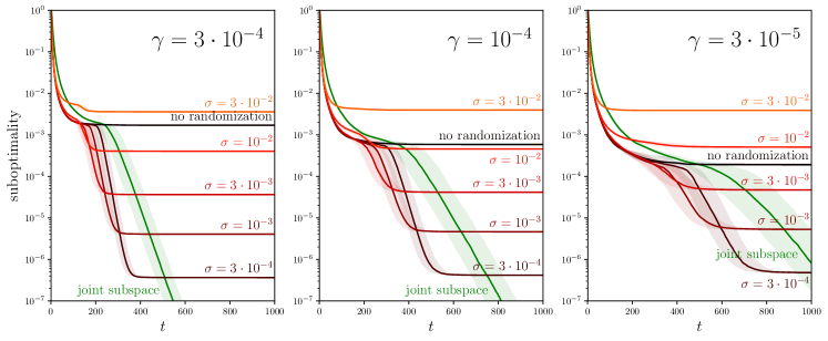
Figure 5: Optimality gap of Krylov subspace solutions on random cubic-regularization problems, versus subspace dimension $t$. Each plot shows result for problem instances with a different eigen-gap $\gamma=(\lambda_{\max}-\lambda_{\min})/(\lambda_{2}-\lambda_{\min})$, where $\lambda_{2}$ is the smallest eigenvalue larger than $\lambda_{\min}$. Each line represents median suboptimality, and shaded regions represent inter-quartile range. Different lines correspond to different randomization settings.

Computing Krylov subspace solutions

We use the Lanczos process to obtain a tridiagonal representation of $A$ as described in Section A. To obtain full optimization traces we solve equation (19) after every Lanczos iteration, warm-starting $\lambda$ with the solution from the previous step and the minimum eigenvalue of the current tridiagonal matrix. We use the Newton method described by Cartis et al. [11, Algorithm 6.1] to solve the equation (19) in the Krylov subspace. For the $\kappa<\infty$ experiment, we stop the process when $|\left\|{A_{\lambda}^{-1}b}\right\|-\lambda/\rho|<10^{-12}$ or after 25 tridiagonal system solves are computed. For the $\kappa=\infty$ experiment we allow up to 100 system solves.

Appendix G Proofs from Section 6

G.1 Proof of Lemma 6.1

Recalling the notation $A_{\star}=A+\rho\left\|{x_{\star}^{\mathsf{cr}}}\right\|I$ and that $(x_{\star}^{\mathsf{cr}})^{T}A_{\star}x_{\star}^{\mathsf{cr}}=-b^{T}x_{\star}^{\mathsf{cr}}$, the minimal value of $f_{A,b,\rho}$ admits the bound

$$f_{A,b,\rho}(x_{\star}^{\mathsf{cr}})=-\frac{1}{2}({x_{\star}^{\mathsf{cr}}})^{T}A_{\star}x_{\star}^{\mathsf{cr}}-\frac{\rho\left\|{x_{\star}^{\mathsf{cr}}}\right\|^{3}}{6}\leq-\frac{\rho\left\|{x_{\star}^{\mathsf{cr}}}\right\|^{3}}{6}.$$

Corollary 5.2 thus implies that the output of $x=\hyperref@@ii[func:SSP]{\textsc{Solve-CR}(A,b,\rho,\beta,\delta)}$ satisfies

$$f_{A,b,\rho}(x) \leq-\frac{1}{6}\rho\left\|{x_{\star}^{\mathsf{cr}}}\right\|^{3}+\frac{\beta\left\|{x_{\star}^{\mathsf{cr}}}\right\|^{2}}{T_{\textup{inner}}^{2}}\left[4+\frac{\mathbb{I}_{\{\lambda_{\min}<0\}}}{2}\log^{2}\left(\frac{4d}{\delta^{2}}\right)\right]$$

$$\leq-\frac{1}{6}\rho\left\|{x_{\star}^{\mathsf{cr}}}\right\|^{3}+\frac{1}{12}\rho r\left\|{x_{\star}^{\mathsf{cr}}}\right\|^{2},$$

where we substituted $T_{\textup{inner}}\geq\sqrt{\frac{12\beta}{\rho r}\left(4+\frac{1}{2}\log^{2}\frac{4d}{\delta^{2}}\right)}$, with probability at least $1-\delta$. Consequently, $\left\|{x_{\star}^{\mathsf{cr}}}\right\|\geq r$ implies $f_{A,b,\rho}(x)\leq-\frac{1}{12}\rho\left\|{x_{\star}^{\mathsf{cr}}}\right\|^{3}\leq-\frac{1}{12}\rho r^{3}$.

G.2 Proof of Lemma 6.2

Let $f(z)=\frac{1}{2}z^{T}(A+2\rho rI)z+b^{T}z$, let $x_{\star}=-(A+2\rho rI)^{-1}b$ be the minimizer of $f$, and let $x=\hyperref@@ii[func:SFSP]{\textsc{Solve-Quadratic}(A,b,\rho,\beta,\varepsilon_{\mathrm{g}})}$. Note that $x$ is the output of $T_{\textup{final}}$ conjugate gradient (CG) steps for minimizing $f$. That $\left\|{x}\right\|\leq\left\|{x_{\star}}\right\|$ holds as CG iterates have nondecreasing norm and converge to $x_{\star}$ [44, Theorem 2.1]. Moreover, bounds on $f(x)-f(x_{\star})$ follow from standard convergence analysis of CG; for convenience we simply apply the first bound of Corollary 4.2 with $\rho=0$, obtaining

$$f(x)-f(x_{\star})\leq 36[f(0)-f(x_{\star})]\exp\left\{-4T_{\textup{final}}\sqrt{\frac{\rho r}{\beta+2\rho r}}\right\}\leq\frac{\varepsilon_{\mathrm{g}}^{2}}{2(\beta+2\rho r)},$$

where we substituted $T_{\textup{final}}\geq\frac{1}{4}\sqrt{\frac{\beta+2\rho r}{\rho r}}\log\frac{36(\beta+2\rho r)^{2}r^{2}}{\varepsilon_{\mathrm{g}}^{2}}$ and $f(0)-f(x_{\star})=\frac{1}{2}x_{\star}^{T}(A+2\rho rI)x_{\star}\leq\frac{1}{2}(\beta+2\rho r)r^{2}$. Using also

$$\left\|{(A+2\rho rI)x+b}\right\|=\left\|{\nabla f(x)}\right\|\leq\sqrt{2(\beta+2\rho r)(f(x)-f(x_{\star}))},$$

we get $\left\|{(A+2\rho rI)x+b}\right\|\leq\varepsilon_{\mathrm{g}}$, whence the final bound $\left\|{Ax+b}\right\|\leq\varepsilon_{\mathrm{g}}+2\rho r^{2}$ follows by substituting $\left\|{x}\right\|\leq r$.

G.3 Proof of Proposition 6.1

The second result is inequality (17). For the first, we argue three facts: first, that the consequences of Lemma 6.1 hold in each call to Solve-CR; second, that when the algorithm terminates it returns an approximate second-order stationary point; and third, that the total number of Hessian-vector products is bounded. We begin with the first. The conclusions of Lemma 6.1 fail in iteration $k$ of Alg. 1 with probability at most $\delta/2k^{2}$, and so a union bound gives

$$\mathbb{P}(\mbox{any failure})\leq\sum_{k=1}^{\infty}\frac{\delta}{2k^{2}}<\delta.$$

We perform our analysis deterministically in the event that no failures occur.

To prove that the algorithm terminates with a second-order stationary point, let $K$ be the iteration at which Alg. 1 fails to make enough progress, that is, $g(y_{K})>g(y_{K-1})-\frac{1}{12}\rho r^{3}$. Let $\Delta^{\star}$ minimize model (16) at $y=y_{K-1}$, and let $\Delta_{\textup{final}}$ be the output of the call to Solve-Quadratic, so that $y_{\textup{final}}=y_{K-1}+\Delta_{\textup{final}}$ is the output of Find-SOSP. The fact that $g(y_{K})>g(y_{K-1})-\frac{1}{12}\rho r^{3}$ implies $\left\|{\Delta^{\star}}\right\|\leq r$ (Lemma 6.1), and since $\nabla^{2}g(y_{K-1})+\rho\left\|{\Delta^{\star}}\right\|I\succeq 0$ by Proposition 2.1, the condition $-\rho rI\preceq\nabla^{2}g(y_{K-1})\preceq\beta I$ of Lemma 6.2 holds for the call Solve-Quadratic. Similarly, Proposition 2.1 requires that $\left\|{(A+\rho\left\|{\Delta^{\star}}\right\|)^{\dagger}b}\right\|\leq\left\|{\Delta^{\star}}\right\|$ and consequently

$$\left\|{(A+2\rho rI)^{-1}b}\right\|\leq\left\|{(A+\rho\left\|{\Delta^{\star}}\right\|)^{\dagger}b}\right\|\leq\left\|{\Delta^{\star}}\right\|\leq r,$$

so that the second condition of Lemma 6.2 holds. Applying the lemma, we obtain

$$\left\|{\Delta_{\textup{final}}}\right\|\leq r~{}~{}\mbox{and}~{}~{}\left\|{\nabla^{2}g(y_{K-1})\Delta_{\textup{final}}+\nabla g(y_{K-1})}\right\|\leq\varepsilon_{\mathrm{g}}+2\rho r^{2}.$$

Now we demonstrate approximate stationarity. Using that $\nabla^{2}g$ is $2\rho$-Lipschitz continuous, the bounds $\nabla^{2}g(y_{K-1})\succeq-\rho rI$ and $\|{\Delta_{\textup{final}}}\|\leq r$, where $r=\sqrt{\epsilon/9\rho}$ imply

$$\nabla^{2}g(y_{\textup{final}})\succeq\nabla^{2}g(y_{k-1})-2\rho\left\|{\Delta_{\textup{final}}}\right\|I\succeq-3\rho rI=-\sqrt{\rho\epsilon}I.$$

To control $y_{\textup{final}}$, let $v=\nabla f_{\nabla^{2}g(y_{K-1}),\nabla g(y_{K-1})}(\Delta_{\textup{final}})=\nabla^{2}g(y_{K-1})\Delta_{\textup{final}}+\nabla g(y_{K-1})$, noting that $\left\|{v}\right\|\leq\varepsilon_{\mathrm{g}}+2\rho r^{2}$ as above. Moreover, the $2\rho$-Lipschitz continuity of $\nabla^{2}g$ implies that $\left\|{\nabla g(y_{\textup{final}})-v}\right\|\leq\rho\left\|{\Delta_{\textup{final}}}\right\|^{2}\leq\rho r^{2}$. Putting these two observations together and using $r=\sqrt{\epsilon/(9\rho)}$ and $\varepsilon_{\mathrm{g}}=2\epsilon/3$, we have the desired stationarity (15):

$$\left\|{\nabla g(y_{\textup{final}})}\right\|\leq\left\|{\nabla g(y_{\textup{final}})-v}\right\|+\left\|{v}\right\|\leq\varepsilon_{\mathrm{g}}+3\rho r^{2}=\varepsilon.$$

For the final component of the proposition, we bound the total number of Hessian-vector products the method requires. The total number of gradient computation and calls to Solve-CR is $T_{\textup{outer}}=K=O(1)\frac{\sqrt{\rho}(g(y_{0})-g_{\star})}{\epsilon^{3/2}}$. The number of Hessian-vector products in each call to Solve-CR is at most

$$\left\lceil{\sqrt{\frac{24\beta}{\rho r}\left(4+\frac{1}{2}\log^{2}\frac{16T_{\textup{outer}}^{4}d}{\delta^{2}}\right)}}\right\rceil=O(1)\frac{\beta^{1/2}}{\rho^{1/4}\epsilon^{1/4}}\log\left[\frac{d}{\delta^{2}}\cdot\frac{\sqrt{\rho}(g(y_{0})-g_{\star})}{\epsilon^{3/2}}\right],$$

where we have used $\epsilon\leq\min\{\beta^{2}/\rho,\rho^{1/3}(g(y_{0})-g_{\star})^{2/3}\}$. Similarly simplifying the number of Hessian-vector product evaluations in the call to Solve-Quadratic gives

$$\frac{1}{4}\sqrt{\frac{\beta+2\rho r}{\rho r}}\log\frac{36(\beta+2\rho r)^{2}r^{2}}{\varepsilon_{\mathrm{g}}^{2}}=O(1)\frac{\beta^{1/2}}{\rho^{1/4}\epsilon^{1/4}}\log\left[\frac{\beta^{1/2}}{\rho^{1/4}\epsilon^{1/4}}\right],$$

and multiplying the last two displays by $T_{\textup{outer}}\leq O(1)\frac{\sqrt{\rho}(g(y_{0})-g_{\star})}{\epsilon^{3/2}}$ implies the proposition.

References

- Agarwal et al. [2017] N. Agarwal, Z. Allen-Zhu, B. Bullins, E. Hazan, and T. Ma. Finding approximate local minima faster than gradient descent. In Proceedings of the Forty-Ninth Annual ACM Symposium on the Theory of Computing, 2017.
- Beck and Vaisbourd [2018] A. Beck and Y. Vaisbourd. Globally solving the trust region subproblem using simple first-order methods. SIAM Journal on Optimization, 28(3):1951–1967, 2018.
- Bianconcini et al. [2015] T. Bianconcini, G. Liuzzi, B. Morini, and M. Sciandrone. On the use of iterative methods in cubic regularization for unconstrained optimization. Computational Optimization and Applications, 60(1):35–57, 2015.
- Bottou et al. [2018] L. Bottou, F. Curtis, and J. Nocedal. Optimization methods for large-scale learning. SIAM Review, 60(2):223–311, 2018.
- Carmon and Duchi [2018] Y. Carmon and J. C. Duchi. Analysis of Krylov subspace solutions of regularized nonconvex quadratic problems. In Advances in Neural Information Processing Systems 31, 2018. URL https://arxiv.org/abs/1806.09222.
- Carmon and Duchi [2019] Y. Carmon and J. C. Duchi. Gradient descent finds the cubic-regularized nonconvex Newton step. SIAM Journal on Optimization, 29(3):2146–2178, 2019.
- Carmon et al. [2017] Y. Carmon, J. C. Duchi, O. Hinder, and A. Sidford. Convex until proven guilty: dimension-free acceleration of gradient descent on non-convex functions. In Proceedings of the 34th International Conference on Machine Learning, 2017.
- Carmon et al. [2018] Y. Carmon, J. C. Duchi, O. Hinder, and A. Sidford. Accelerated methods for non-convex optimization. SIAM Journal on Optimization, 28(2):1751–1772, 2018.
- Carmon et al. [2019] Y. Carmon, J. C. Duchi, O. Hinder, and A. Sidford. Lower bounds for finding stationary points I. Mathematical Programming, Series A, to appear, 2019.
- Cartis et al. [2011a] C. Cartis, N. I. Gould, and P. L. Toint. Adaptive cubic regularisation methods for unconstrained optimization. Part II: worst-case function-and derivative-evaluation complexity. Mathematical Programming, Series A, 130(2):295–319, 2011a.
- Cartis et al. [2011b] C. Cartis, N. I. M. Gould, and P. L. Toint. Adaptive cubic regularisation methods for unconstrained optimization. Part I: motivation, convergence and numerical results. Mathematical Programming, Series A, 127:245–295, 2011b.
- Coakley and Rokhlin [2013] E. S. Coakley and V. Rokhlin. A fast divide-and-conquer algorithm for computing the spectra of real symmetric tridiagonal matrices. Applied and Computational Harmonic Analysis, 34(3):379–414, 2013.
- Conn et al. [2000] A. R. Conn, N. I. M. Gould, and P. L. Toint. Trust Region Methods. MPS-SIAM Series on Optimization. SIAM, 2000.
- Cullum and Donath [1974] J. Cullum and W. E. Donath. A block Lanczos algorithm for computing the q algebraically largest eigenvalues and a corresponding eigenspace of large, sparse, real symmetric matrices. In 13th IEEE Conference on Decisions and Control, pages 505–509. IEEE, 1974.
- Ge et al. [2015] R. Ge, F. Huang, C. Jin, and Y. Yuan. Escaping from saddle points—online stochastic gradient for tensor decomposition. In Proceedings of the Twenty Eighth Annual Conference on Computational Learning Theory, 2015.
- Ge et al. [2016] R. Ge, J. D. Lee, and T. Ma. Matrix completion has no spurious local minimum. In Advances in Neural Information Processing Systems 29, 2016.
- Ge et al. [2017] R. Ge, C. Jin, and Y. Zheng. No spurious local minima in nonconvex low rank problems: A unified geometric analysis. In Proceedings of the 34th International Conference on Machine Learning, 2017.
- Golub and Loan [1989] G. Golub and C. V. Loan. Matrix Computations. John Hopkins University Press, 1989.
- Golub and Underwood [1977] G. H. Golub and R. Underwood. The block Lanczos method for computing eigenvalues. In Mathematical software, pages 361–377. Elsevier, 1977.
- Gould et al. [1999] N. I. M. Gould, S. Lucidi, M. Roma, and P. L. Toint. Solving the trust-region subproblem using the Lanczos method. SIAM Journal on Optimization, 9(2):504–525, 1999.
- Griewank [1981] A. Griewank. The modification of Newton’s method for unconstrained optimization by bounding cubic terms. Technical report, Technical report NA/12, 1981.
- Hardt et al. [2018] M. Hardt, T. Ma, and B. Recht. Gradient descent learns linear dynamical systems. Journal of Machine Learning Research, 19(1):1025–1068, 2018.
- Hazan and Koren [2016] E. Hazan and T. Koren. A linear-time algorithm for trust region problems. Mathematical Programming, Series A, 158(1):363–381, 2016.
- Hestenes and Stiefel [1952] M. Hestenes and E. Stiefel. Methods of conjugate gradients for solving linear systems. Journal of Research of the National Bureau of Standards, 49(6), 1952.
- Ho-Nguyen and Kılınc̨-Karzan [2017] N. Ho-Nguyen and F. Kılınc̨-Karzan. A second-order cone based approach for solving the trust-region subproblem and its variants. SIAM Journal on Optimization, 27(3):1485–1512, 2017.
- Kohler and Lucchi [2017] J. M. Kohler and A. Lucchi. Sub-sampled cubic regularization for non-convex optimization. In Proceedings of the 34th International Conference on Machine Learning, 2017.
- Kuczynski and Wozniakowski [1992] J. Kuczynski and H. Wozniakowski. Estimating the largest eigenvalue by the power and Lanczos algorithms with a random start. SIAM Journal on Matrix Analysis and Applications, 13(4):1094–1122, 1992.
- Li and Yuan [2017] Y. Li and Y. Yuan. Convergence analysis of two-layer neural networks with ReLU activation. In Advances in Neural Information Processing Systems 30, pages 597–607, 2017.
- Ma et al. [2019] C. Ma, K. Wang, Y. Chi, and Y. Chen. Implicit regularization in nonconvex statistical estimation: Gradient descent converges linearly for phase retrieval, matrix completion and blind deconvolution. Foundations of Computational Mathematics, to appear, 2019.
- Martens and Grosse [2015] J. Martens and R. Grosse. Optimizing neural networks with kronecker-factored approximate curvature. In Proceedings of the 32nd International Conference on Machine Learning, pages 2408–2417, 2015.
- Martínez [1994] J. M. Martínez. Local minimizers of quadratic functions on Euclidean balls and spheres. SIAM Journal on Optimization, 4(1):159–176, 1994.
- Murty and Kabadi [1987] K. Murty and S. Kabadi. Some NP-complete problems in quadratic and nonlinear programming. Mathematical Programming, 39:117–129, 1987.
- Nemirovski [1994] A. Nemirovski. Efficient methods in convex programming. Technion: The Israel Institute of Technology, 1994.
- Nemirovski and Yudin [1983] A. Nemirovski and D. Yudin. Problem Complexity and Method Efficiency in Optimization. Wiley, 1983.
- Nesterov [1983] Y. Nesterov. A method of solving a convex programming problem with convergence rate . Soviet Mathematics Doklady, 27(2):372–376, 1983.
- Nesterov [2004] Y. Nesterov. Introductory Lectures on Convex Optimization. Kluwer Academic Publishers, 2004.
- Nesterov and Polyak [2006] Y. Nesterov and B. Polyak. Cubic regularization of Newton method and its global performance. Mathematical Programming, Series A, 108:177–205, 2006.
- Nocedal and Wright [2006] J. Nocedal and S. J. Wright. Numerical Optimization. Springer, 2006.
- Pearlmutter [1994] B. A. Pearlmutter. Fast exact multiplication by the Hessian. Neural Computation, 6(1):147–160, 1994.
- Royer and Wright [2018] C. W. Royer and S. J. Wright. Complexity analysis of second-order line-search algorithms for smooth nonconvex optimization. SIAM Journal on Optimization, 28(2):1448–1477, 2018.
- Royer et al. [2019] C. W. Royer, M. O’Neill, and S. J. Wright. A Newton-CG algorithm with complexity guarantees for smooth unconstrained optimization. Mathematical Programming, Series A, 2019.
- Schraudolph [2002] N. N. Schraudolph. Fast curvature matrix-vector products for second-order gradient descent. Neural Computation, 14(7):1723–1738, 2002.
- Simchowitz et al. [2018] M. Simchowitz, A. E. Alaoui, and B. Recht. Tight query complexity lower bounds for PCA via finite sample deformed Wigner law. In Proceedings of the Fiftieth Annual ACM Symposium on the Theory of Computing, 2018.
- Steihaug [1983] T. Steihaug. The conjugate gradient method and trust regions in large scale optimization. SIAM Journal on Numerical Analysis, 20(3):626–637, 1983.
- Sun et al. [2018] J. Sun, Q. Qu, and J. Wright. A geometric analysis of phase retrieval. Foundations of Computational Mathematics, 18(5):1131–1198, 2018.
- Tao and An [1998] P. D. Tao and L. T. H. An. A D.C. optimization algorithm for solving the trust-region subproblem. SIAM Journal on Optimization, 8(2):476–505, 1998.
- Trefethen and Bau III [1997] L. N. Trefethen and D. Bau III. Numerical Linear Algebra. SIAM, 1997.
- Tripuraneni et al. [2018] N. Tripuraneni, M. Stern, C. Jin, J. Regier, and M. I. Jordan. Stochastic cubic regularization for fast nonconvex optimization. In Advances in Neural Information Processing Systems 31, 2018.
- Tseng [2008] P. Tseng. On accelerated proximal gradient methods for convex-concave optimization. 2008. URL http://www.mit.edu/~dimitrib/PTseng/papers/apgm.pdf.
- Weiser et al. [2007] M. Weiser, P. Deuflhard, and B. Erdmann. Affine conjugate adaptive Newton methods for nonlinear elastomechanics. Optimisation Methods and Software, 22(3):413–431, 2007.
- Xu et al. [2019] P. Xu, F. Roosta, and M. W. Mahoney. Newton-type methods for non-convex optimization under inexact Hessian information. Mathematical Programming, Series A, to appear, 2019.
- Zhang et al. [2017] L.-H. Zhang, C. Shen, and R.-C. Li. On the generalized Lanczos trust-region method. SIAM Journal on Optimization, 27(3):2110–2142, 2017.