Closure Properties for Private Classification and Online Prediction

Abstract

Let $\mathcal{H}$ be a class of boolean functions and consider a composed class $\mathcal{H}^{\prime}$ that is derived from $\mathcal{H}$ using some arbitrary aggregation rule (for example, $\mathcal{H}^{\prime}$ may be the class of all 3-wise majority-votes of functions in $\mathcal{H}$). We upper bound the Littlestone dimension of $\mathcal{H}^{\prime}$ in terms of that of $\mathcal{H}$. As a corollary, we derive closure properties for online learning and private PAC learning.

The derived bounds on the Littlestone dimension exhibit an undesirable exponential dependence. For private learning, we prove close to optimal bounds that circumvents this suboptimal dependency. The improved bounds on the sample complexity of private learning are derived algorithmically via transforming a private learner for the original class $\mathcal{H}$ to a private learner for the composed class $\mathcal{H}^{\prime}$. Using the same ideas we show that any (proper or improper) private algorithm that learns a class of functions $\mathcal{H}$ in the realizable case (i.e., when the examples are labeled by some function in the class) can be transformed to a private algorithm that learns the class $\mathcal{H}$ in the agnostic case.

1 Introduction

We study closure properties for learnability of binary-labeled hypothesis classes in two related settings: online learning and differentially private PAC learning.

Closure Properties for Online Learning.

Let $\mathcal{H}$ be a class of experts that can be online learned with vanishing regret. That is, there exists an algorithm $\mathcal{A}$ such that given any sequence of $T$ prediction tasks, the number of false predictions made by $\mathcal{A}$ is larger by at most $R(T)=o(T)$ than the number of false predictions made by the best expert in $\mathcal{H}$.

Consider a scenario where the sequence of tasks is such that every single expert in $\mathcal{H}$ predicts poorly on it, however there is a small unknown set of experts $h_{1},\ldots,h_{k}\in\mathcal{H}$ that can predict well by collaborating. More formally, there is an aggregation rule $G:\{0,1\}^{k}\to\{0,1\}$ such that the combined expert $G(h_{1},\ldots,h_{k})$ exhibits accurate predictions on a significant majority of the tasks. For example, a possible aggregation rule $G$ could be the majority-vote of the $k$ experts. Since we assume that the identities of the $k$ experts are not known, it is natural to consider the class $\mathcal{H}^{\prime}=\{G(h_{1},\ldots,h_{k}):h_{i}\in\mathcal{H}\},$ which consists of all possible $G$-aggregations of $k$ experts from $\mathcal{H}$. We study the following question:

Question 1.1.

Can the optimal regret with respect to $\mathcal{H}^{\prime}$ be bounded in terms of that of $\mathcal{H}$?

The Littlestone dimension is a combinatorial parameter that determines online learnability (Littlestone, 1987; Ben-David et al., 2009). In particular, $\mathcal{H}$ is online learnable if and only if it has a finite Littlestone dimension $d<\infty$, and the best possible regret $R(T)$ for online learning $\mathcal{H}$ satisfies

$$\Omega(\sqrt{dT})\leq R(T)\leq O(\sqrt{dT\log T}).$$ (1)

Furthermore, if it is known that if one of the experts never errs (a.k.a the realizable setting), then the optimal regret is exactly $d$. (The regret is called mistake-bound in this context.)

Thus, the above question boils down to asking whether the Littlestone dimension of $\mathcal{H}^{\prime}$ is bounded by a function of the Littlestone dimension of $\mathcal{H}$. One of the two main results in this work provides an affirmative answer to this question (Theorem 2.1).

We next discuss a variant of this question in the setting of Differentially Private (DP) learning. The two settings of online and DP-learning are intimately related (see, e.g., Bun et al. (2020); Abernethy et al. (2017); Joseph et al. (2019); Gonen et al. (2019)). In particular, both online learning and DP-learning are characterized by the finiteness of the Littlestone dimension (Littlestone, 1987; Ben-David et al., 2009; Bun et al., 2015; Alon et al., 2019; Bun et al., 2020).

Closure Properties for Differentially Private Learning.

Imagine the following medical scenario: consider a family $\mathcal{H}$ of viruses for which there is an algorithm $\mathcal{A}$ that can learn to diagnose any specific virus $h\in\mathcal{H}$ given enough labeled medical data. Further assume that $\mathcal{A}$ has the desired property of being differentially private learning algorithm as defined by (Kasiviswanathan et al., 2011); that is, it is a PAC learning algorithm in which the privacy of every patient whose data is used during training is guarded in the formal sense of differential privacy (Dwork et al., 2006b).

Assume that an outbreak of a deadly disease $h^{\prime}$ has occurred in several locations all over the world and that it is known that $h^{\prime}$ is caused by some relatively small, yet unknown group of viruses from $\mathcal{H}$. That is, our prior information is that there are unknown viruses $h_{1},\ldots,h_{k}\in\mathcal{H}$ for a relatively small $k$ such that $h^{\prime}=G(h_{1},\ldots,h_{k})$ for some rule $G$. For example, $G$ could be the OR function in which case $h^{\prime}$ occurs if and only if the patient is infected with at least one of the viruses $h_{1},\ldots,h_{k}$.

It would be highly beneficial if one could use the algorithm $\mathcal{A}$ to diagnose $h^{\prime}$ in an automated fashion. Moreover, doing it in a private manner could encourage health institutions in the different locations to contribute their patients’ data. This inspires the following question:

Question 1.2.

Can one use the algorithm $\mathcal{A}$ to privately learn to diagnose $h^{\prime}$? How does the sample complexity of this learning task scale as a function of $G$?

Differential Privacy, Online Learning, and the Littlestone Dimension.

Question 1.2 and Question 1.1 are equivalent in the sense that both online learning and DP-learning are characterized by the finiteness of the Littlestone dimension (Littlestone, 1987; Ben-David et al., 2009; Bun et al., 2015; Alon et al., 2019; Bun et al., 2020).

Note however that unlike the bounds relating the Littlestone dimension to online learning, which are tight up to logarithmic factors (see 1), the bounds relating the Littlestone dimension and DP-learning are very far from each other; specifically, if $d$ denotes the Littlestone dimension of $\mathcal{H}$ then the lower bound on the sample complexity of privately learning $\mathcal{H}$ scales with $\log^{*}d$ (Bun et al., 2015; Alon et al., 2019), while the best known upper bound scales with $\exp(d)$ (Bun et al., 2020).

Thus, while our solution to Question 1.1 yields an affirmative answer to Question 1.2, the implied quantitative bounds are far from being realistically satisfying. Specifically, every finite $\mathcal{H}$ is learnable with privacy using $O(\log|\mathcal{H}|)$ samples (Kasiviswanathan et al., 2011), and so if $\mathcal{H}$ is finite and not too large, the bounds implied by the Littlestone dimension are not meaningful. We therefore focus on deriving effective bounds for private learning, which is the content of Theorem 2.3 (see Theorem 7.1 for a precise statement).

Littlestone Classes.

It is natural to ask which natural hypothesis classes have bounded Littlestone dimension. First, it holds that $\mathrm{Ldim}(\mathcal{H})\leq\log\lvert\mathcal{H}\rvert$ for every $\mathcal{H}$, so for finite classes the Littlestone dimension scales rather gracefully with their size.

There are also natural infinite Littlestone classes: for example, let the domain $X=\mathbb{F}^{n}$ be an $n$-dimensional vector space over some field $\mathbb{F}$ and let $\mathcal{H}\subseteq\{0,1\}^{X}$ consist of all affine subspaces of $V$ of dimension $\leq d$. It can be shown here that $\mathrm{Ldim}(\mathcal{H})=d$. (For example, the class of all lines in $\mathbb{R}^{100}$ has Littlestone dimension $1$.) A bit more generally, any class of hypotheses that can be described by polynomial equalities of a bounded degree has bounded Littlestone dimension. (Observe that if one replaces “equalities” with “inequalities” then the Littlestone dimension may become unbounded, however the VC dimension remains bounded (e.g. Halfspaces).) We note in passing that this can be further generalized to classes that are definable in stable theories, which is a deep and well-explored notion in model theory. We refer the reader to Chase and Freitag (2019), Section 5.1 for such examples.

Organization.

Formal statement of our main results and description of our techniques appears in Section 2, specifically, a short overview of the proofs is given in Section 2.1. Definitions and background results are provided in Section 3. The complete proofs appear in the rest of the paper. Closure properties for Littlestone classes is proved in Section 4. The effective bounds for private learning are given in Section 5 and Sections 6 and 7. We note that each of these parts can be read independently of the other.

2 Main Results and Techniques

Let $G:\{0,1\}^{k}\to\{0,1\}$ be a boolean function and let $\mathcal{H}_{1},\ldots,\mathcal{H}_{k}\subseteq\{0,1\}^{X}$ be hypothesis classes. Denote by $G(\mathcal{H}_{1},\ldots,\mathcal{H}_{k})$ the following class $G(\mathcal{H}_{1},\ldots,\mathcal{H}_{k})=\{G(h_{1},\ldots,h_{k}):h_{i}\in\mathcal{H}_{i}\}.$ For example, if $G(x_{1},x_{2})=x_{1}\land x_{2}$ then $G(\mathcal{H}_{1},\mathcal{H}_{2})=\mathcal{H}_{1}\land\mathcal{H}_{2}=\{h_{1}\land h_{2}:h_{i}\in\mathcal{H}_{i}\}$ is the class of all pairwise intersections/conjunctions of a function from $\mathcal{H}_{1}$ and a function from $\mathcal{H}_{2}$.

Theorem 2.1 (A Closure Theorem for the Littlestone Dimension).

Let $G:\{0,1\}^{k}\to\{0,1\}$ be a boolean function, let $\mathcal{H}_{1},\ldots,\mathcal{H}_{k}\subseteq\{0,1\}^{X}$ be classes, and let $d\in\mathbb{N}$ such that $\mathrm{Ldim}(\mathcal{H}_{i})\leq d$ for every $i\leq k$. Then,

$$\mathrm{Ldim}(G(\mathcal{H}_{1},\ldots,\mathcal{H}_{k}))\leq\tilde{O}(2^{2k}k^{2}d),$$

where $\tilde{O}$ conceals polynomial factors in $\log k$ and $\log d$.

In particular, if $\mathrm{Ldim}(\mathcal{H}_{i})<\infty$ for all $i\leq d$ then $\mathrm{Ldim}(G(\mathcal{H}_{1},\ldots,\mathcal{H}_{k}))<\infty$. Consequently, if each of the $\mathcal{H}_{i}$’s is online learnable then $G(\mathcal{H}_{1},\ldots,\mathcal{H}_{k})$ is online learnable. We comment that if the aggregating function $G$ is simple then one can obtain better bounds. For example, if $G$ is a majority-vote, a $k$-wise OR, or a $k$-wise AND function then a bound of $\tilde{O}(k^{2}\cdot d)$ holds. (See Section 4.2.2.)

Another combinatorial parameter which arises in the relationship between online and DP learning is the threshold dimension: a sequence $x_{1},\ldots,x_{k}\in X$ is threshold-shattered by $\mathcal{H}$ if there are $h_{1},\ldots,h_{k}\in\mathcal{H}$ such that $h_{i}(x_{j})=1$ if and only if $i\leq j$ for all $i,j\leq k$. The threshold dimension, $T(\mathcal{H})$ is the maximum size of a sequence that is threshold-shattered by $\mathcal{H}$. The threshold dimension plays a key role in showing that DP learnable classes have a finite Littlestone dimension (Alon et al., 2019). A classical theorem by Shelah (1978) in model theory shows that the Littlestone and the threshold dimensions are exponentially related. In particular $\mathrm{Ldim}(\mathcal{H})<\infty$ if and only if $T(\mathcal{H})<\infty$. (See Theorem 3.2 in the preliminaries section.) We prove the following closure theorem in terms of the threshold dimension.

Theorem 2.2 (A Closure Theorem for the Threshold Dimension).

Let $G:\{0,1\}^{k}\to\{0,1\}$ be a boolean function, let $\mathcal{H}_{1},\ldots,\mathcal{H}_{k}\subseteq\{0,1\}^{X}$ be classes, and let $t\in\mathbb{N}$ such that $T(\mathcal{H}_{i})<t$ for every $i\leq k$. Then,

$$T\bigl{(}G(\mathcal{H}_{1},\ldots,\mathcal{H}_{k})\bigr{)}<2^{4k4^{k}\cdot t}.$$

Moreover, an exponential dependence in $t$ is necessary: for every $t\geq 6$ there exists a class $\mathcal{H}$ such that $T(\mathcal{H})\leq t$ and

$$T\Bigl{(}\{h_{1}\lor h_{2}:h_{1},h_{2}\in\mathcal{H}\}\Bigr{)}\geq 2^{\lfloor t/5\rfloor}.$$

Note that the bounds in Theorem 2.1 and Theorem 2.2 escalate rapidly with $k$ (the arity of $G$) and with $t$. It will be interesting to determine tight bounds.

By Alon et al. (2019); Bun et al. (2020), Theorem 2.1 also implies closure properties for DP-learnable classes. However, the quantitative bounds are even worse: not only do the bounds on the Littlestone dimension of $G(\mathcal{H}_{1},\ldots,\mathcal{H}_{k})$ escalate rapidly with $d$ and $k$, also the quantitative relationship between the Littlestone dimension and DP-learning sample complexity is very loose, and the best bounds exhibit a tower-like gap between the upper and lower bounds. For example, if the class of functions $\mathcal{H}$ is finite and its Littlestone dimension is $\omega(\log\log|\mathcal{H}|)$, then the bound of Theorem 2.1 is most likely to be much worse than the generic application of the exponential mechanism, whose sample complexity is the logarithm of the size of the class. We therefore explore the closure properties of differentially-private learning algorithms directly and derive the following bound.

Theorem 2.3 (A Closure Theorem for Private Learning (informal)).

Let $G:\{0,1\}^{k}\to\{0,1\}$ be a boolean function. Let $\mathcal{H}_{1},\ldots,\mathcal{H}_{k}\subseteq\{0,1\}^{X}$ be classes that are $(\varepsilon,\delta)$-differentially private and $(\alpha,\beta)$-accurate learnable with sample complexity $m_{i}$ respectively. Then, $G(\mathcal{H}_{1},\ldots,\mathcal{H}_{k})$ is $(\varepsilon,\delta)$-private and $(\alpha,\beta)$-accurate learnable with sample complexity

$$\tilde{O}\left(\sum_{i=1}^{k}m_{i}\right)\cdot\operatorname*{\mathrm{poly}}(k,1/\varepsilon,1/\alpha,\log(1/\beta)).$$

The exact quantitative satement of the results appears in Theorem 7.1. We remark that closure properties for pure differentially-private learning algorithms (i.e., when $\delta=0$) are implied by the characterization of (Beimel et al., 2019). Similarly, closure properties for non-private PAC learning are implied by the characterization of their sample complexity in terms of the VC dimension and by the Sauer-Shelah-Perles Lemma (Sauer, 1972). However, since there is no tight characterization of the sample complexity of approximate differentially-private learning algorithms (i.e., when $\delta>0$), we prove Theorem 2.3 algorithmically by constructing a (non-efficient) learning algorithm for $G(\mathcal{H}_{1},\ldots,\mathcal{H}_{k})$ from private learning algorithms for $\mathcal{H}_{1},\ldots,\mathcal{H}_{k}$.

Beimel et al. (2015) proved that any proper private learning algorithm in the realizable case can be transformed into an agnostic private learning algorithm, with only a mild increase in the sample complexity. We show that the same result holds even for improper private learning (i.e., when the private learning algorithm can return an arbitrary hypothesis).

Theorem 2.4 (Private Learning Implies Agnostic Private Learning).

For every $0<\alpha,\beta,\delta<1$, every $m\in{\mathbb{N}}$, and every concept class $\mathcal{H}$, if there exists a $(1,\delta)$-differentially private $(\alpha,\beta)$-accurate PAC learner for the hypothesis class $\mathcal{H}$ with sample complexity $m$, then there exists an $(O(1),O(\delta))$-differentially private $(O(\alpha),O(\beta+\delta n))$-accurate agnostic learner for $\mathcal{H}$ with sample complexity

$$n=O\Bigg{(}m+\frac{1}{\alpha^{2}}\left(\operatorname{\rm VC}(\mathcal{H})+\log\frac{1}{\beta}\right)\Bigg{)}.$$

Furthermore, if the original learner is proper, then the agnostic learner is proper.

We obtain this result by showing that a variant of the transformation of (Beimel et al., 2015) also works for the improper case; we do not know if the original transformation of (Beimel et al., 2015) also works for the improper case. Our analysis of the transformation for the improper case is more involved than the analysis for the proper case.

2.1 Technical Overview

2.1.1 Closure for Littlestone Dimension

Our proof of Theorem 2.1 exploits tools from online learning. It may be instructive to compare Theorem 2.1 with an analogous result for VC classes: a classical result by Dudley (1978) upper bounds the VC dimension of $G(\mathcal{H}_{1},\ldots,\mathcal{H}_{k})$ by $\tilde{O}(d_{1}+\cdots+d_{k})$, where $d_{i}$ is the VC dimension of $\mathcal{H}_{i}$. The argument uses the Sauer-Shelah-Perles Lemma (Sauer, 1972) to bound the growth-rate (a.k.a. shatter function) of $G(\mathcal{H}_{1},\ldots,\mathcal{H}_{k})$ by some $n^{d_{1}+\cdots+d_{k}}$: indeed, if we let $n=\operatorname{\rm VC}(G(\mathcal{H}_{1},\ldots,\mathcal{H}_{k})),$ then by the definition of the shatter function, $2^{n}\leq n^{d_{1}+\cdots+d_{k}}$, which implies that $n=\tilde{O}(d_{1}+\cdots+d_{k})$ as stated. It is worth noting that a notion of growth-rate as well as a corresponding variant of the Sauer-Shelah-Perles Lemma also exist for Littlestone classes (Bhaskar, 2017; Chase and Freitag, 2018). However we are not aware of a way of using it to prove Theorem 2.1.

We take a different approach. We first focus on the case where $G$ is a majority-vote. That is, the class $\mathcal{H}=G(\mathcal{H}_{1},\ldots,\mathcal{H}_{k})$ consists of all $k$-wise majority-votes of experts $h_{i}\in\mathcal{H}_{i}$. We bound the Littlestone dimension of $\mathcal{H}$ by exhibiting an online learning algorithm $A$ that learns $\mathcal{H}$ in the mistake-bound model with at most $\tilde{O}(k^{2}\cdot d)$ mistakes. The derivation of $A$ exploits fundamental tools from online learning such as the Weighted Majority Algorithm by Littlestone and Warmuth (1989) and Online Boosting (Chen et al., 2012; Beygelzimer et al., 2015; Brukhim et al., 2020).

Then, the bound for a general $G:\{0,1\}^{k}\to\{0,1\}$ is obtained by expressing $G$ as a formula which only uses majority-votes and negations gates. The exponential dependence in $k$ in the final bound is a consequence of the formula-size which can be exponential in $k$. We do not know whether this exponential dependence is necessary.

2.1.2 Closure for Threshold Dimension

Our proof of Theorem 2.2 is combinatorial. First, note that an inferior bound follows from Theorem 2.1, using the fact that the Littlestone and threshold dimensions are exponentially related (see Theorem 3.2). However this approach yields a super-exponential bound on $T(G(\mathcal{H}_{1},\ldots,\mathcal{H}_{k}))$.

The bound in Theorem 2.2 follows by arguing contra-positively that if $T(G(\mathcal{H}_{1},\ldots,\mathcal{H}_{k}))$ is large then $T(\mathcal{H}_{i})$ is also “largish” for some $i\leq k$. Specifically, if $T(G(\mathcal{H}_{1},\ldots,\mathcal{H}_{k}))\geq\exp(t\exp(k))$ then $T(\mathcal{H}_{i})\geq t$ for some $i\leq k$. This is shown using a Ramsey argument that asserts that any large enough sequence $x_{1},\ldots,x_{n}$ that is threshold-shattered by $G(\mathcal{H}_{1}\ldots\mathcal{H}_{k})$ must contain a relatively large subsequence that is threshold-shattered by one of the $\mathcal{H}_{i}$’s. Quantitatively, if $n\geq\exp(t\exp(k))$ then there must be a subsequence $x_{j_{1}},\ldots,x_{j_{t}}$ that is threshold-shattered by one of the $\mathcal{H}_{i}$’s.

This upper bounds $T(G(\mathcal{H}_{1},\ldots,\mathcal{H}_{k}))$ by some $\exp(t\exp(k))$, where $t=\max_{i}T(\mathcal{H}_{i})$. It is worth noting that, in contrast with Theorem 2.1, an exponential dependence here is inevitable: we prove in Theorem 2.2 that for any $t$ there exists a class $\mathcal{H}$ with $T(\mathcal{H})\leq t$ such that $T(\{h_{1}\lor h_{2}:h_{1},h_{2}\in\mathcal{H}\})\geq\exp(t)$. This lower bound is achieved by a randomized construction.

2.1.3 Private learning Implies Agnostic Private Learning

We start by describing the transformation of (Beimel et al., 2015) from a proper private learning algorithm of a class $\mathcal{H}$ to an agnostic proper private learning algorithm for $\mathcal{H}$. Assume that there is a private learning algorithm $\mathcal{A}$ for $\mathcal{H}$ with sample complexity $m$. The transformation takes a sample $S$ of size $O(m)$ and constructs all possible behaviors $H$ of functions in $\mathcal{H}$ on the points of the sample (ignoring the labels). By the Sauer-Shelah-Perles Lemma, the number of such behaviors is at most $\left(\frac{e|S|}{\operatorname{\rm VC}(\mathcal{H})}\right)^{\operatorname{\rm VC}(\mathcal{H})}$. Then, it finds using the exponential mechanism a behavior $h^{\prime}\in H$ that minimizes the empirical error on the sample. (The exponential mechanism is guaranteed to identify a behavior with small empirical error because the number of possible behaviors is relatively small.) Finally, the transformation relabeles the sample $S$ using $h^{\prime}$ and applies $\mathcal{A}$ on the relabeled sample. If $\mathcal{A}$ is a proper learning algorithm then, by standard VC arguments, the resulting algorithm is an agnostic algorithm for $\mathcal{H}$. The privacy guarantees of the resulting algorithm are more delicate, and it is only $O(1)$-differentially private, even if $\mathcal{A}$ is $\varepsilon$-differentially private for a small $\varepsilon$. (The difficulty in the privacy analysis is the set of behaviors $H$ is data-dependent. Therefore, the privacy guarantees of the resulting algorithms are not directly implied by those of the exponential mechanism, which assume that the set of possible outcomes is fixed and data-independent.)

When $\mathcal{A}$ is improper, we cannot use VC arguments to argue that the resulting algorithm is an agnostic learner. We rather use the generalization properties of differential privacy (proved in (Dwork et al., 2015; Bassily et al., 2016; Rogers et al., 2016; Feldman and Steinke, 2017; Nissim and Stemmer, 2017; Jung et al., 2020)): if a differentially private algorithm has a small empirical error on a sample chosen i.i.d. from some distribution, then it also has a small generalization error on the underlying distribution (even if the labeling hypothesis is chosen after seeing the sample). There are technical issues in applying these results in our case that require some modifications in the transformation.

2.1.4 Closure for Differentially Private Learning

We prove Theorem 2.3 by constructing a private algorithm $\mathcal{A}_{\rm ClosureLearn}$ for the class $G(\mathcal{H}_{1},\ldots,\mathcal{H}_{k})$ using private learning algorithms for the classes $\mathcal{H}_{1},\ldots,\mathcal{H}_{k}$. Algorithm $\mathcal{A}_{\rm ClosureLearn}$ uses the relabeling procedure (the one that we use to transform a private PAC learner into a private agnostic learner) in a new setting.

The input to $\mathcal{A}_{\rm ClosureLearn}$ is a sample labeled by some function in $G(\mathcal{H}_{1},\ldots,\mathcal{H}_{k})$. The algorithm finds hypotheses $h_{1},\ldots,h_{k}$ in steps, where in the $i$’th step, the algorithm finds a hypothesis $h_{i}$ such that $h_{1},\dots,h_{i}$ have a completion $c_{i+1},\dots,c_{k}$ to a hypothesis $G(h_{1},\dots,h_{i},c_{i+1},\dots,c_{k})$ with small error (assuming that $h_{1},\dots,h_{i-1}$ have a good completion).

Each step of $\mathcal{A}_{\rm ClosureLearn}$ is similar to the algorithm for agnostic learning described above. That is, in the $i$’th step, $\mathcal{A}_{\rm ClosureLearn}$ first relabels the input sample $S$ using some $h\in\mathcal{H}_{i}$ in a way that guarantees completion to a hypothesis with small empirical error. The relabeling $h$ is chosen using the exponential mechanism with an appropriate score function. The relabeled sample is then fed to the private algorithm for the class $\mathcal{H}_{i}$ to produce a hypothesis $h_{i}$ and then the algorithm proceeds to the next step $i+1$. As in the algorithm for agnostic learning, the proof that the hypothesis $G(h_{1},\ldots,h_{k})$ returned by the algorithm is easier when the private algorithms for $\mathcal{H}_{1},\ldots,\mathcal{H}_{k}$ are proper and it is more involved if they are improper.

3 Preliminaries

This section is organized as follows: Section 3.1 contains basic definitions and tools related to the Littlestone dimension and Section 3.2 contains basic definitions and tools related to private learning.

3.1 Preliminaries on the Littlestone Dimension

The Littlestone dimension is a combinatorial parameter that characterizes regret bounds in online learning (Littlestone, 1987; Ben-David et al., 2009). The definition of this parameter uses the notion of mistake-trees: these are binary decision trees whose internal nodes are labeled by elements of $X$. Any root-to-leaf path in a mistake tree can be described as a sequence of examples $(x_{1},y_{1}),\ldots,(x_{d},y_{d})$, where $x_{i}$ is the label of the $i$’th internal node in the path, and $y_{i}=$ if the $(i+1)$’th node in the path is the right child of the $i$’th node, and otherwise $y_{i}=0$. We say that a tree $T$ is shattered by $\mathcal{H}$ if for any root-to-leaf path $(x_{1},y_{1}),\ldots,(x_{d},y_{d})$ in $T$ there is $h\in\mathcal{H}$ such that $h(x_{i})=y_{i}$, for all $i\leq d$. The Littlestone dimension of $\mathcal{H}$, denoted by $\mathrm{Ldim}(\mathcal{H})$, is the depth of the largest complete tree that is shattered by $\mathcal{H}$.

Definition 3.1 (Subtree).

Let $T$ be labeled binary tree. We will use the following notion of a subtree $T^{\prime}$ of depth $h$ of $T$ by induction on $h$:

1. Any leaf of $T$ is a subtree of height $0$.

2. For $h\geq 1$ a subtree of height $h$ is obtained from an internal vertex of $T$ together with a subtree of height $h-1$ of the tree rooted at its left child and a subtree of height $h-1$ of the tree rooted at its right child.

Note that if $T$ is a labeled tree and it is shattered by the class $\mathcal{H}$, then any subtree $T^{\prime}$ of it with the same labeling of its internal vertices is shattered by the class $\mathcal{H}$.

Threshold Dimension.

A classical theorem of Shelah in model-theory connects bounds on 2-rank (Littlestone dimension) to the concept of thresholds: let $\mathcal{H}\subseteq\{0,1\}^{X}$ be a hypothesis class. We say that a sequence $x_{1},\ldots,x_{k}\in X$ is threshold-shattered by $\mathcal{H}$ if there are $h_{1},\ldots,h_{k}\in\mathcal{H}$ such that $h_{i}(x_{j})=1$ if and only if $i\leq j$ for all $i,j\leq k$. Define the threshold dimension, $T(\mathcal{H})$, as the maximum size of a sequence that is threshold-shattered by $\mathcal{H}$.

Theorem 3.2 (Littlestone Dimension versus Threshold Dimension (Shelah, 1978; Hodges, 1997)).

Let $\mathcal{H}$ be a hypothesis class, then:

$$T(\mathcal{H})\geq\lfloor\log\mathrm{Ldim}(\mathcal{H})\rfloor~{}~{}\text{ and }~{}~{}\mathrm{Ldim}(\mathcal{H})\geq\lfloor\log T(\mathcal{H})\rfloor.$$

3.2 Preliminaries on Private Learning

Differential Privacy.

Consider a database where each record contains information of an individual. An algorithm is said to preserve differential privacy if a change of a single record of the database (i.e., information of an individual) does not significantly change the output distribution of the algorithm. Intuitively, this means that the information inferred about an individual from the output of a differentially-private algorithm is similar to the information that would be inferred had the individual’s record been arbitrarily modified or removed. Formally:

Definition 3.3 (Differential privacy (Dwork et al., 2006b, a)).

A randomized algorithm $\mathcal{A}$ is $(\varepsilon,\delta)$-differentially private if for all neighboring databases $S_{1},S_{2}\in X^{m}$ (i.e., databases differing in one entry), and for all sets $\mathcal{F}$ of outputs,

$$\Pr[\mathcal{A}(S_{1})\in\mathcal{F}]\leq\exp(\varepsilon)\cdot\Pr[\mathcal{A}(S_{2})\in\mathcal{F}]+\delta,$$ (2)

where the probability is taken over the random coins of $\mathcal{A}$. When $\delta=0$ we omit it and say that $\mathcal{A}$ preserves pure $\varepsilon$-differential privacy. When $\delta>0$, we use the term approximate differential privacy , in which case $\delta$ is typically a negligible function of the database size $m$.

PAC Learning.

We next define the probably approximately correct (PAC) model of Valiant (1984). A hypothesis $c:X\rightarrow\{0,1\}$ is a predicate that labels examples taken from the domain $X$ by either 0 or 1. We sometime refer to a hypothesis as a concept. A hypothesis class $\mathcal{H}$ over $X$ is a set of hypotheses (predicates) mapping $X$ to $\{0,1\}$. A learning algorithm is given examples sampled according to an unknown probability distribution $\mathcal{P}$ over $X$, and labeled according to an unknown target concept $c\in\mathcal{H}$. The learning algorithm is successful when it outputs a hypothesis $h$ that approximates the target concept over samples from $\mathcal{P}$. More formally:

Definition 3.4.

The generalization error of a hypothesis $h:X\rightarrow\{0,1\}$ with respect to a concept $c$ and a distribution $\mathcal{P}$ over $X$ is defined as ${\rm error}_{\mathcal{P}}(c,h)=\Pr_{x\sim\mathcal{P}}[h(x)\neq c(x)].$ If ${\rm error}_{\mathcal{P}}(c,h)\leq\alpha$ we say that $h$ is $\alpha$-good for $c$ and $\mathcal{P}$.

Definition 3.5 (PAC Learning (Valiant, 1984)).

An algorithm $\mathcal{A}$ is an $(\alpha,\beta)$-accurate PAC learner for a hypothesis class $\mathcal{H}$ over $X$ if for all concepts $c\in\mathcal{H}$, all distributions $\mathcal{P}$ on $X$, given an input of $m$ samples $S=(z_{1},\ldots,z_{m})$, where $z_{i}=(x_{i},c(x_{i}))$ and each $x_{i}$ is drawn i.i.d. from $\mathcal{P}$, algorithm $\mathcal{A}$ outputs a hypothesis $h$ satisfying

$$\Pr[{\rm error}_{\mathcal{P}}(c,h)\leq\alpha]\geq 1-\beta,$$

where the probability is taken over the random choice of the examples in $S$ according to $\mathcal{P}$ and the random coins of the learner $\mathcal{A}$. If the output hypothesis $h$ always satisfies $h\in\mathcal{H}$ then $\mathcal{A}$ is called a proper PAC learner; otherwise, it is called an improper PAC learner.

Definition 3.6.

For an unlabeled sample $S=(x_{i})_{i=1}^{m}$, the empirical error of two concepts $c,h$ is ${\rm error}_{S}(c,h)=\frac{1}{m}|\{i:c(x_{i})\neq h(x_{i})\}|.$ For a labeled sample $S=(x_{i},y_{i})_{i=1}^{m}$, the empirical error of $h$ is ${\rm error}_{S}(h)=\frac{1}{m}|\{i:h(x_{i})\neq y_{i}\}|.$

The previous definition of PAC learning captures the realizable case, that is, the examples are drawn from some distribution and labeled according to some concept $c\in\mathcal{H}$. We next define agnostic learning, i.e., where there is a distribution over labeled examples and the goal is to find a hypothesis whose error is close to the error of the best hypothesis in $\mathcal{H}$ with respect to the distribution. Formally, for a distribution $\mu$ on $X\times\{0,1\}$ and a function $f:X\rightarrow\{0,1\}$ we define ${\rm error}_{\mu}(f)=\Pr_{(x,a)\sim\mu}[f(x)\neq a]$.

Definition 3.7 (Agnostic PAC Learning).

Algorithm $\mathcal{A}$ is an $(\alpha,\beta)$-accurate agnostic PAC learner for a hypothesis class $\mathcal{H}$ with sample complexity $m$ if for all distributions $\mu$ on $X\times\{0,1\}$, given an input of $m$ labeled samples $S=(z_{1},\ldots,z_{m})$, where each labeled example $z_{i}=(x_{i},a_{i})$ is drawn i.i.d. from $\mu$, algorithm $\mathcal{A}$ outputs a hypothesis $h\in\mathcal{H}$ satisfying

$$\Pr\left[\left\lvert{\rm error}_{\mu}(h)-\min_{c\in\mathcal{H}}\{{\rm error}_{\mu}(c)\}\right\rvert\leq\alpha\right]\geq 1-\beta,$$

where the probability is taken over the random choice of the examples in $S$ according to $\mu$ and the random coins of the learner $\mathcal{A}$. If the output hypothesis $h$ always satisfies $h\in\mathcal{H}$ then $\mathcal{A}$ is called a proper agnostic PAC learner; otherwise, it is called an improper agnostic PAC learner.

The following bound is due to (Vapnik and Chervonenkis, 1971; Blumer et al., 1989).

Theorem 3.8 (VC-Dimension Generalization Bound).

Let $\mathcal{H}$ and $\mathcal{P}$ be a concept class and a distribution over a domain $X$. Let $\alpha,\beta>0$, and

$$m\geq\frac{80}{\alpha}\left(\operatorname{\rm VC}(\mathcal{H})\ln\left(\frac{16}{\alpha}\right)+\ln\left(\frac{2}{\beta}\right)\right).$$

Suppose that we draw an unlabeled sample $S=(x_{i})_{i=1}^{m}$, where $x_{i}$ are drawn i.i.d. from $\mathcal{P}$. Then,

$$\Pr[\exists c,h\in\mathcal{H}\text{ s.t. }{\rm error}_{\mathcal{P}}(h,c)>\alpha\;\wedge\;{\rm error}_{S}(h)<\alpha/2]\leq\beta.$$

The next theorem, due to (Vapnik and Chervonenkis, 1971; Anthony and Bartlett, 2009; Anthony and Shawe-Taylor, 1993), handles (in particular) the agnostic case.

Theorem 3.9 (VC-Dimension Agnostic Generalization Bound).

There exists a constant $\gamma$ such that for every domain $X$, every concept class $\mathcal{H}$ over the domain $X$, and every distribution $\mu$ over the domain $X\times\{0,1\}$: For a sample $S=(x_{i},y_{i})_{i=1}^{m}$ where

$$m\geq\gamma\frac{\operatorname{\rm VC}(\mathcal{H})+\ln(\frac{1}{\beta})}{\alpha^{2}}$$

and $\{(x_{i},y_{i})\}$ are drawn i.i.d.  from $\mu$, it holds that

$$\Pr\Big{[}\exists\;h\in\mathcal{H}\text{ s.t. }\big{|}{\rm error}_{\mu}(h)-{\rm error}_{S}(h)\big{|}\geq\alpha\Big{]}\leq\beta.$$

Notice that in Theorem 3.9 the sample complexity is proportional to $\frac{1}{\alpha^{2}}$, as opposed to $\frac{1}{\alpha}$ in Theorem 3.8.

Private Learning.

Consider an algorithm $\mathcal{A}$ in the probably approximately correct (PAC) model of Valiant (1984). We say that $\mathcal{A}$ is a private learner if it also satisfies differential privacy w.r.t. its training data.

Definition 3.10 (Private PAC Learning (Kasiviswanathan et al., 2011)).

Let $\mathcal{A}$ be an algorithm that gets an input $S=(z_{1},\ldots,z_{m})$, where each $z_{i}$ is a labeled example. Algorithm $\mathcal{A}$ is an $(\varepsilon,\delta)$-differentially private $(\alpha,\beta)$-accurate PAC learner with sample complexity $m$ for a class $\mathcal{H}$ over $X$ if

Privacy. Algorithm $\mathcal{A}$ is $(\varepsilon,\delta)$-differentially private (as in Definition 3.3);

Utility. and Algorithm $\mathcal{A}$ is an $(\alpha,\beta)$-accurate PAC learner for $\mathcal{H}$ with sample complexity $m$ (as in Definition 3.5).

When $\delta=0$ (pure privacy) we omit it from the list of parameters.

Note that the utility requirement in the above definition is an average-case requirement, as the learner is only required to do well on typical samples. In contrast, the privacy requirement is a worst-case requirement that must hold for every pair of neighboring databases (no matter how they were generated).

The following definition and lemma are taken from Bun et al. (2015).

Definition 3.11 (Empirical Learner).

Algorithm $\mathcal{A}$ is an $(\alpha,\beta)$-accurate empirical learner for a class $\mathcal{H}$ over $X$ with sample complexity $m$ if for every $c\in\mathcal{H}$ and for every sample $S$ of size $m$ that is labeled by $c$, the algorithm $\mathcal{A}$ outputs a hypothesis $h\in H$ satisfying

$$\Pr[{\rm error}_{S}(c,h)\leq\alpha]\geq 1-\beta.$$

Lemma 3.12 (Bun et al. (2015)).

Suppose $\mathcal{A}$ is an $(\varepsilon,\delta)$-differentially private $(\alpha,\beta)$-accurate PAC learner for a concept class $\mathcal{H}$ with sample complexity $m$. Let $\mathcal{A}^{\prime}$ be an algorithm, whose input sample $S$ contains $9m$ randomly labeled examples. Further assume that $\mathcal{A}^{\prime}$ samples with repetitions $m$ labeled examples from $S$ and returns the output of $\mathcal{A}$ on these examples. Then, $\mathcal{A}^{\prime}$ is an $(\varepsilon,\delta)$-differentially private $(\alpha,\beta)$-accurate empirical learner for $\mathcal{H}$ with sample complexity $9m$. Clearly, if $\mathcal{A}$ is proper, then so is $\mathcal{A}^{\prime}$.

The Exponential Mechanism.

We next describe the exponential mechanism of McSherry and Talwar (2007). Let $X$ be a domain and $H$ a set of solutions. Given a score function $q:X^{*}\times H\rightarrow{\mathbb{N}}$, and a database $S\in X^{*}$, the goal is to chooses a solution $h\in H$ approximately minimizing $q(S,h)$. The mechanism chooses a solution probabilistically, where the probability mass that is assigned to each solution $h$ decreases exponentially with its score $q(S,h)$:

Algorithm 1 $\mathcal{A}_{\rm ExponentialMechanism}$

Input: parameter $\varepsilon$, finite solution set $H$, database $S\in X^{m}$, and a sensitivity 1 score function $q$ (i.e., $|q(D)-q(D^{\prime})|\leq 1$ for every neighboring $D,D^{\prime}\in X^{m}$).

1. Randomly choose $h\in H$ with probability $\frac{\exp\left(-\varepsilon\cdot q(S,h)/2\right)}{\sum_{f\in H}\exp\left(-\varepsilon\cdot q(S,f)/2\right)}.$

2. Output $h$.

Proposition 3.13 (Properties of the Exponential Mechanism).

(i) The exponential mechanism is $\varepsilon$-differentially private. (ii) Let $\hat{e}\triangleq\min_{f\in H}\{q(S,f)\}$ and $\Delta>0$. The exponential mechanism outputs a solution $h$ such that $q(S,h)\geq(\hat{e}+\Delta m)$ with probability at most $|H|\cdot\exp(-\varepsilon\Delta m/2)$.

Kasiviswanathan et al. (2011) showed that the exponential mechanism can be used as a generic private learner – when used with the score function $q(S,h)=|\{i:h(x_{i})\neq y_{i}\}|=m\cdot{\rm error}_{S}(h)$, the probability that the exponential mechanism outputs a hypothesis $h$ such that ${\rm error}_{S}(h)>\min_{f\in H}\{{\rm error}_{S}(f)\}+\Delta$ is at most $|H|\cdot\exp(-\varepsilon\Delta m/2)$. This results in a generic private proper-learner for every finite concept class $\mathcal{H}$, with sample complexity $O_{\alpha,\beta,\varepsilon}(\log|\mathcal{H}|)$.

Generalization Properties of Differentially Private Algorithms.

In this paper we use the fact that differential privacy implies generalization (Dwork et al., 2015; Bassily et al., 2016; Rogers et al., 2016; Feldman and Steinke, 2017; Nissim and Stemmer, 2017; Jung et al., 2020): differentially private learning algorithms satisfy that their empirical loss is typically close to their population loss. We use the following variant of this result, which is a multiplicative version that applies also to the case that $\varepsilon>1$ (as needed in this paper).

Theorem 3.14 (DP Generalization – Multiplicative version (Dwork et al., 2015; Bassily et al., 2016; Feldman and Steinke, 2017; Nissim and Stemmer, 2017)).

Let $\mathcal{A}$ be an $(\varepsilon,\delta)$-differentially private algorithm that operates on a database of $S\in X^{n}$ and outputs a predicate $\operatorname{\rm test}:X\rightarrow\{0,1\}$. Let $\mathcal{P}$ be a distribution over $X$ and $S$ be a database containing $n$ i.i.d.  elements from $\mathcal{P}$. Then,

$$\Pr_{\begin{subarray}{c}S\in_{\mbox{\tiny R}}X^{n},\\ \operatorname{\rm test}\leftarrow_{R}\mathcal{A}(S)\end{subarray}} \left[\operatorname*{\mathbb{E}}_{x\in_{\mathcal{P}}X}[\operatorname{\rm test}(x)]>e^{2\varepsilon}\left(\frac{\sum_{x\in S}\operatorname{\rm test}(x)}{n}+\frac{10}{\varepsilon n}\log\left(\frac{1}{\varepsilon\delta n}\right)\right)\right]<O\left(\frac{\varepsilon\delta n}{\log(\frac{1}{\varepsilon\delta n})}\right).$$

4 Closure of Littlestone Classes

In this section we study closure properties for Littlestone classes. We begin in Section 4.1 with a rather simple (and tight) analysis of the behavior of the Littlestone and Threshold dimension under unions. Then, in Section 4.2 we prove our main results in this part (Theorems 2.1 and 2.2) which bound the variability of the Littlestone and Thresholds dimension under arbitrary compositions.

4.1 Closure Under Unions

We begin with two basic bounds on the variability of the Littlestone/Threshold dimension under union. Note that here $\mathcal{H}_{1}\cup\mathcal{H}_{2}$ denotes the usual union: $\mathcal{H}_{1}\cup\mathcal{H}_{2}=\{h:h\in\mathcal{H}_{1}\text{ or }h\in\mathcal{H}_{2}\}$. These bounds are useful as they allows us to reduce a bound on the dimension of $G(\mathcal{H}_{1},\mathcal{H}_{2})$ for arbitrary $\mathcal{H}_{1},\mathcal{H}_{2}$ to the case where $\mathcal{H}_{1}=\mathcal{H}_{2}$ (because $G(\mathcal{H}_{1},\mathcal{H}_{2})\subseteq G(\mathcal{H},\mathcal{H})$ for $\mathcal{H}=\mathcal{H}_{1}\cup\mathcal{H}_{2}$).

Observation 4.1.

[Threshold Dimension Under Union] Let $\mathcal{H}_{1},\mathcal{H}_{2}\subseteq\{0,1\}^{X}$ be hypothesis classes with $T(\mathcal{H}_{i})=t_{i}$. Then,

$$T(\mathcal{H}_{1}\cup\mathcal{H}_{2})\leq t_{1}+t_{2}.$$

Moreover, this bound is tight: for every $t_{1},t_{2}$, there are classes $\mathcal{H}_{1},\mathcal{H}_{2}$ with Threshold dimension $t_{1},t_{2}$ respectively such that $T(\mathcal{H}_{1}\cup\mathcal{H}_{2})=t_{1}+t_{2}$.

Proof.

For the upper bound, observe that if $h_{1}\ldots h_{m}\in\mathcal{H}_{1}\cup\mathcal{H}_{2}$ threshold-shatters the sequence $x_{1}\ldots x_{m}$ then $\{h_{i}:h_{i}\in\mathcal{H}_{j}\}$ threshold-shatters $\{x_{i}:h_{i}\in\mathcal{H}_{j}\}$ for $j\in\{1,2\}$. For the lower bound, set $X=[t_{1}+t_{2}]$, $\mathcal{H}_{1}=\{h_{i}:i\leq t_{1}\}$, and $\mathcal{H}_{2}=\{h_{i}:t_{1}<i\leq t_{1}+t_{2}\}$, where $h_{i}(j)=1$ if and only if $i\leq j$. ∎

Proposition 4.2 (Littlestone Dimension Under Union).

Let $\mathcal{H}_{1},\mathcal{H}_{2}\subseteq\{0,1\}^{X}$ be hypothesis classes with $\mathrm{Ldim}(\mathcal{H}_{i})=d_{i}$. Then,

$$\mathrm{Ldim}(\mathcal{H}_{1}\cup\mathcal{H}_{2})\leq d_{1}+d_{2}+1.$$

Moreover, this bound is tight: for every $d_{1},d_{2}$, there are classes $\mathcal{H}_{1},\mathcal{H}_{2}$ with Littlestone dimension $d_{1},d_{2}$ respectively such that $\mathrm{Ldim}(\mathcal{H}_{1}\cup\mathcal{H}_{2})=d_{1}+d_{2}+1$.

Proof of 4.2.

There are several ways to prove this statement. One possibility is to use the realizable online mistake-bound setting (Littlestone, 1987) and argue that $\mathcal{H}_{1}\cup\mathcal{H}_{2}$ can be learned with at most $d_{1}+d_{2}+1$ mistakes in this setting. We present here an alternative inductive argument, which may be of independent interest. Towards this end, it is convenient to define the depth of the empty tree as $-1$, and that of a tree consisting of one vertex (leaf) as $0$.

Consider a shattered tree $T$ of depth $d=\mathrm{Ldim}(\mathcal{H}_{1}\cup\mathcal{H}_{2})$ with leaves labelled $\mathcal{H}_{1}$ and $\mathcal{H}_{2}$ in the obvious way. Recall the notion of a subtree in Definition 3.1, and let $x\leq\mathrm{Ldim}(\mathcal{H}_{1})$ be the maximum depth of a complete binary subtree all whose leaves are $\mathcal{H}_{1}$ leaves, and $y\leq\mathrm{Ldim}(\mathcal{H}_{2})$ the maximum depth of a subtree all whose leaves are $\mathcal{H}_{2}$-leaves. Similarly, let $x_{L},y_{L}$ denote the maximum depth of a $\mathcal{H}_{1}$-subtree and a $\mathcal{H}_{2}$-subtree in the tree rooted at the left child of the root of $T$, and let $x_{R},y_{R}$ be the same for the tree rooted at the right child.

It suffices to show that $x+y\geq d-1$: clearly $x\geq\max(x_{L},x_{R})$ and also $x\geq\min(x_{L},x_{R})+1$ thus $x\geq(x_{L}+x_{R})/2+1/2$. Similarly $y\geq(y_{L}+y_{R})/2+1/2$, hence

$$x+y\geq\frac{x_{L}+y_{L}}{2}+\frac{x_{R}+y_{R}}{2}+1$$

and this gives by induction on $d$ (starting with $d=0$ or $1$) that $x+y\geq d-1$ as required.

To see that this bound is tight, pick $n\geq d_{1}+d_{2}+1$ and set

$$\mathcal{H}_{1}=\Big{\{}h:[n]\to\{\pm 1\}\ :\sum_{i}h_{i}\leq d_{1}\Bigr{\}}~{}~{}\text{ and }~{}~{}\mathcal{H}_{1}=\Big{\{}h:[n]\to\{\pm 1\}\ :\sum_{i}h_{i}\geq n-d_{2}\Bigr{\}}.$$

One can verify that $\mathrm{Ldim}(\mathcal{H}_{i})=d_{i}$, for $i=1,2$ and that $\mathrm{Ldim}(\mathcal{H}_{1}\cup\mathcal{H}_{2})=d_{1}+d_{2}+1$, as required (in fact, even the VC dimension of $\mathcal{H}_{1}\cup\mathcal{H}_{2}$ is $d_{1}+d_{2}+1$). ∎

4.2 implies that $\mathrm{Ldim}(\cup_{i=1}^{k}\mathcal{H}_{i})=O(k\cdot d)$ provided that $\mathrm{Ldim}(\mathcal{H}_{i})\leq d$ for al $i$, and that this inequality can be tight when $k=2$. The following proposition shows that for a larger $k$ this bound can be significantly improved:

Proposition 4.3 (Littlestone Dimension Under Multiple Unions).

Let $\mathcal{H}_{1},\ldots,\mathcal{H}_{k}\subseteq\{0,1\}^{X}$ be hypothesis classes with $\mathrm{Ldim}(\mathcal{H}_{i})\leq d$. Then, for every $0<\varepsilon<1/2$,

$$\mathrm{Ldim}(\bigcup_{i=1}^{k}\mathcal{H}_{i}) \leq 3d+3\log k.$$

Moreover, this bound is tight up to a constant factor: for every $k$, there are classes $\mathcal{H}_{1},\ldots,\mathcal{H}_{k}$ with $\mathrm{Ldim}(\mathcal{H}_{i})\leq d$ such that $\mathrm{Ldim}(\cup_{i}\mathcal{H}_{i})\geq d+\lfloor\log k\rfloor$.

4.3 demonstrates a difference with the threshold dimension. Indeed, while the bound above scales logarithmically with $k$, in the case of the threshold dimension a linear dependence in $k$ is necessary: indeed, set $X=[k\cdot t]$, $\mathcal{H}_{i}=\{h_{j}:(i-1)\cdot t<ji\leq i\cdot t\}$, where $h_{i}(j)=1$ if and only if $i\leq j$. Thus, $\mathrm{Ldim}(\mathcal{H}_{i})=t$ for all $i$ and $\mathrm{Ldim}(\cup_{i=1}^{k}\mathcal{H}_{i})=k\cdot t>>t+\log k$.

Proof of 4.3.

We begin with the lower bound: pick any class $\mathcal{H}\subseteq\{0,1\}^{X}$ with Littlestone dimension $d$, and let $T$ be a tree of depth $d$ which is shattered by $\mathcal{H}$. Pick $\lfloor\log k\rfloor$ new points $z_{1},\ldots,z_{\lfloor\log k\rfloor}\notin X$, and extend the domain $X$ to $X^{\prime}=X\cup\{z_{1}\ldots,z_{\lfloor\log k\rfloor}\}$. Define $\mathcal{H}^{\prime}\subseteq\{0,1\}^{X^{\prime}}$ by extending each $h\in\mathcal{H}$ to the $z_{i}$’s in each of the $k^{\prime}=2^{\lfloor\log k\rfloor}$ possible ways. (So, each $h\in\mathcal{H}$ has $k^{\prime}$ copies in $\mathcal{H}^{\prime}$, one for each possible pattern on the $z_{i}$’s.) Thus, $\mathcal{H}^{\prime}$ is a union of $k^{\prime}$ copies of $\mathcal{H}$, one copy for each boolean pattern on the $z_{i}$’s. In particular, $\mathcal{H}^{\prime}$ is the union of $k^{\prime}$ classes with Littlestone dimension $d$. Also note that $\mathrm{Ldim}(\mathcal{H}^{\prime})\geq\lfloor\log k\rfloor+d$, as witnessed by the tree which is illustrated in Figure 1.

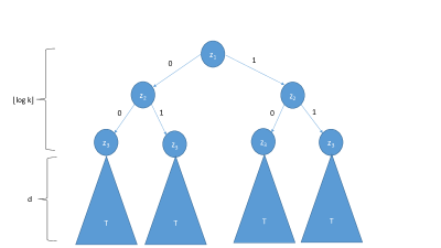
Figure 1: An illustration of the tree shattered by $\mathcal{H}^{\prime}$ in the construction in 4.3. In this illustration $\lfloor\log k\rfloor$ equals 3.

The upper bound is based on a multiplicative-weights argument. Recall that the Littlestone dimension equals the optimal number of mistakes performed by a deterministic online learner in the mistake-bound model (i.e. online learning when the sequence of input examples is labelled by some $h\in\mathcal{H}$). Thus, it suffices to demonstrate an online learner for $\cup_{i=1}^{k}\mathcal{H}_{i}$ which makes at most $3d+3\log k$ mistakes. Pick for every $\mathcal{H}_{i}$ an online learner $A_{i}$ which makes at most $d$ mistakes on input sequences consistent with $\mathcal{H}_{i}$. We set the online learning algorithm $A$ for $\mathcal{H}=\cup_{i=1}^{k}\mathcal{H}_{i}$ to be The Weighted Majority Algorithm by Littlestone and Warmuth (1989) with the $k$ experts being the algorithms $A_{1},\ldots,A_{k}$. Now, consider an input sequence $S=(x_{1},y_{1}),\ldots(x_{T},y_{T})$ consistent with $\mathcal{H}$. Thus, $S$ is consistent with $\mathcal{H}_{i}$ for some $i\leq k$ and therefore $A_{i}$ makes at most $d$ mistakes on it. Thus, by the multiplicative weights analysis (see e.g. Corollary 2.1 in Littlestone and Warmuth (1989)), the number of mistakes $A$ makes on $S$ is at most

$$\frac{\log k+d\log\frac{1}{\beta}}{\log\frac{2}{1+\beta}},$$

where $0\leq\beta<1$ is multiplicative factor which discounts the weights of wrong experts. The upper bound follows by setting $\beta=1/2$.

∎

4.2 Closure Under Composition

4.2.1 Threshold Dimension

Proof of Theorem 2.1.

We begin with the upper bound. Let $T(G(\mathcal{H}_{1},\ldots,\mathcal{H}_{k}))=n$. It suffices to show that if $n\geq 2^{4k4^{k}\cdot t}$ then there is $i\leq k$ such that $T(\mathcal{H}_{i})\geq t$. By assumption, there are $x_{1},x_{2}\ldots x_{n}\in X$ and functions $h_{ij}\in\mathcal{H}_{j}$, for $1\leq i\leq n,1\leq j\leq k$ such that

$$(\forall i,j\leq n):G(h_{i1},h_{i2},\ldots,h_{ik})(x_{j})=1\iff i\leq j.$$

Construct a coloring of the edges of the complete graph on $[n]$ by $4^{k}$ colors as follows: for each $1\leq p<q\leq n$, the color of the edge $\{p,q\}$ is given by the following ordered sequence of $2k$ bits:

$$\bigl{(} h_{p,1}(x_{q}),h_{p,2}(x_{q}),\ldots,h_{p,k}(x_{q}),$$

$$h_{q,1}(x_{p}),h_{q,2}(x_{p}),\ldots,h_{q,k}(x_{p})\bigr{)}.$$

By Ramsey Theorem (Ramsey, 1930), if $n\geq(4^{k})^{2t\cdot 4^{k}}=2^{4k4^{k}\cdot t}$ then there is a monochromatic set $A\subseteq[n]$ of size $\lvert A\rvert=2t$. Denote the elements of $A$ by

$$A=\{i_{1}<j_{1}<i_{2}<j_{2}<\ldots<i_{t}<j_{t}\},$$

and let $u=(u_{1}\ldots u_{k})$, $v=(v_{1}\ldots v_{k})$ such that the color of every pair in $A$ is

$$( v_{1},v_{2},\ldots,v_{k},$$

$$u_{1},u_{2},\ldots,u_{k}).$$

Thus, for every pair $p,q\leq d$ and every $r\leq k$:

$$h_{i_{p},r}(x_{j_{q}})=\begin{cases}v_{r}&p\leq q\\ u_{r}&p>q.\end{cases}$$

We claim that $u\neq v$: indeed, $x_{j_{1}},x_{j_{2}},x_{j_{3}},\ldots,x_{j_{t}}$ is threshold-shattered by the functions

$$G(h_{i_{1},1},h_{i_{1},2},\ldots,h_{i_{1},k}),G(h_{i_{2},1},h_{i_{2},2},\ldots,h_{i_{2},k}),\cdots G(h_{i_{d},1},h_{i_{d},2},\ldots,h_{i_{t},k}).$$

Thus,

$$p\leq q \implies G(v)=G(h_{i_{p},1}\ldots h_{i_{p},k})(x_{q})=1,$$

$$p>q \implies G(u)=G(h_{i_{p},1}\ldots h_{i_{p},k})(x_{q})=0.$$

Therefore, $v\in G^{-1}(0)$ and $u\in G^{-1}(1)$ and in particular $u\neq v$. Pick an index $r$ so that $u_{r}\neq v_{r}$. Therefore, for every $p,q\leq t$:

$$h_{i_{p},r}(x_{j_{q}})=\begin{cases}v_{r}&p\leq q\\ u_{r}&p>q,\end{cases}\text{and}~{}~{}~{}v_{r}\neq u_{r}.$$

This shows that either $x_{1}\ldots x_{t}$ is threshold shattered by $\mathcal{H}_{r}$ (if $v_{r}=1,u_{r}=0$), or $x_{t}\ldots x_{1}$ is thresholds shattered by $\mathcal{H}_{r}$ (if $v_{r}=0,u_{r}=1$); in either way, the threshold dimension of $\mathcal{H}_{r}$ is at least $t$. This completes the proof of the upper bound.

Lower Bound.

We next prove the lower bound. Let $m=2^{\lfloor t/5\rfloor}$, and construct $\mathcal{H}\subseteq\{0,1\}^{m}$ randomly as follows: $\mathcal{H}$ consists of $2m$ random functions

$$\mathcal{H}=\{f_{1}\ldots f_{m},g_{1}\ldots g_{m}\},$$

where for each $i$ set $f_{i}(j)=g_{j}(j)=0$ for $j>i$, and for $j\leq i$, pick uniformly at random one of $f_{i},g_{i}$, set it to be $1$ in position $j$ and set the other to be $0$ in position $j$. All of the above ${m-1\choose 2}$ random choices are done independently. By construction, $\{h_{1}\lor h_{2}:h_{1},h_{2}\in\mathcal{H}\}$ threshold-shatters the sequence $1,2\ldots,m$ with probability $1$ and hence has threshold dimension at least $m$. It suffices to show that with a positive probability it holds that

$$T(\mathcal{H})\leq 2k,$$ (3)

where $k=(2+\frac{1}{\log m})\log m=2\lfloor t/5\rfloor+1$. Indeed, $2k=4\lfloor t/5\rfloor+2\leq t$ whenever $t\geq 6$.

We set out to prove 3. Consider the following event:

$\mathcal{E}:=$ There exist no $x_{1},\ldots,x_{k}\in[m]$, $h_{1},\ldots h_{k}\in\mathcal{H}$ such that $h_{i}(x_{j})=1$ for all $i,j\leq k$.

Note that $\mathcal{E}$ implies that $T(\mathcal{H})\leq 2k$ and therefore it suffices to show that $\Pr[E]>0$. Towards this end we use a union bound: we define a family of “bad” events whose total sum of probabilities is less than one with the property that if none of the bad events occurs then $\mathcal{E}$ occurs. The bad events are defined as follows: for any pair of subsets $A,B\subseteq[m]$ of size $\lvert A\rvert=\lvert B\rvert=k$, let $\mathcal{B}_{A,B}$ denote the event

$\mathcal{B}_{A,B}:=$ “For every $i\in A$ there exists $r_{i}\in\{f_{i},g_{i}\}$ such that $r_{i}(j)=1$ for all $j\in B$.”

Note that indeed $\lnot\mathcal{E}$ implies $\mathcal{B}_{A,B}$ for some $A,B$ and thus it suffices to show that with a positive probability none of the $\mathcal{B}_{A.B}$ occurs. We claim that

$$\Pr[\mathcal{B}_{A,B}]\leq 2^{-k(k-1)}.$$

Indeed, for a fixed $i\in A$, the probability that one of $f_{i},g_{i}$ equals to $1$ on all $j\in B$ is at most $2^{-(k-1)}$. By independence, the probability that the latter simultaneously holds for every $i\in A$ is at most $2^{-k(k-1)}$. Thus, the probability that $\mathcal{B}_{A,B}$ occurs for at least one pair $A,B$ is at most

$${m\choose k}^{2}2^{-k(k-1)}<2^{2k\log m-k(k-1)}\leq 1,$$

where the last inequality holds because $k=(2+\frac{1}{\log m})\log m$.

∎

4.2.2 Littlestone Dimension

Proof of Theorem 2.1.

We will first show that for an odd $k$, the majority-vote $G=\mathsf{MAJ}_{k}$ satisfies

$$\mathrm{Ldim}(\mathsf{MAJ}_{k}(\mathcal{H}_{1}\ldots\mathcal{H}_{k}))\leq\tilde{O}(k^{2}\cdot d).$$ (4)

(Recall that $d=\max_{i}\mathrm{Ldim}(\mathcal{H}_{i})$.) Then, we use this to argue that for any $G$,

$$\mathrm{Ldim}(G(\mathcal{H}_{1}\ldots\mathcal{H}_{k}))\leq\tilde{O}(2^{2k}k^{2}d).$$ (5)

We start with proving 4. Let $\mathcal{H}=\cup_{i=1}^{k}\mathcal{H}_{i}$ and $\mathcal{H}_{k}=\mathsf{MAJ}_{k}(\mathcal{H},\ldots,\mathcal{H})$. Since $\mathsf{MAJ}_{k}(\mathcal{H}_{1},\ldots,\mathcal{H}_{k})\subseteq\mathcal{H}_{k}$, it suffices to show that $\mathrm{Ldim}(\mathcal{H}_{k})\leq\tilde{O}(k^{2}d)$. We use online boosting towards this end.

Online boosting (in the realizable setting) is an algorithmic framework which allows to transform a weak online learner for $\mathcal{H}$ with a non-trivial mistake-bound of $({1}/{2}-\gamma)T+R(T)$, where $R(T)=o(T)$ is a sublinear regret function, to a strong online learner with a vanishing mistake-bound of $O(R(T)/\gamma)$. Online boosting has been studied by several works (e.g. Chen et al. (2012); Beygelzimer et al. (2015); Brukhim et al. (2020)). We use here the variant given by Brukhim et al. (2020) (see Theorem 2 there).

Which weak learner to use? Recall that by Ben-David et al. (2009) (see Equation 1) there exists an agnostic online learning algorithm $W$ for $\mathcal{H}$ whose (expected) regret bound is

$$R(T)=O(\sqrt{\mathrm{Ldim}(\mathcal{H})T\log T}).$$

We claim that $W$ is a weak learner for $\mathcal{H}_{k}$ with mistake-bound

$$(1/2-1/k)\cdot T+R(T).$$ (6)

To prove this, it suffices to show that for every sequence of examples $(x_{1},y_{1})\ldots(x_{T},y_{T})$ which is consistent with $\mathcal{H}_{k}$ there exists $h\in\mathcal{H}$ which makes at most $(1/2-1/k)\cdot T$ mistakes on it. Indeed, let $h_{1}\ldots h_{k}$ such that $y_{t}=\mathsf{MAJ}_{k}(h_{1}(x_{t})\ldots h_{k}(x_{t}))$ for $t\leq T$. Thus, on every example $(x_{t},y_{t})$ at most $1/2-1/k$ fraction of the $h_{i}$’s make a mistake on it. By averaging, this implies that one of the $h_{i}$ makes at most $(1/2-1/k)T$ mistakes in total, and 6 follows.

Now, by applying online boosting with $W$ as a weak learner, we obtain an algorithm with a mistake-bound of at most

$$O\Bigl{(}\frac{R(T)}{1/k}\Bigr{)}=O\Bigl{(}k\sqrt{\mathrm{Ldim}(\mathcal{H})T\log T}\Bigr{)}.$$

Thus, since the Littlestone dimension characterizes the optimal mistake-bound, letting $D=\mathrm{Ldim}(\mathcal{H}_{k})$, we get that

$$(\forall T\geq D):D\leq O\Bigl{(}k\sqrt{\mathrm{Ldim}(\mathcal{H})T\log T}\Bigr{)},$$

and in particular $D\leq O\Bigl{(}k\sqrt{\mathrm{Ldim}(\mathcal{H})D\log D}\Bigr{)}$, which implies that

$$D \leq\tilde{O}(k^{2}\mathrm{Ldim}(\mathcal{H}))$$

$$\leq\tilde{O}k^{2}d+k^{2}\log k)$$ (4.3)

$$=\tilde{O}(k^{2}d),$$

and finishes the proof of 4.

We next set out to prove 5. The idea is to represent an arbitrary $G$ using a formula which only uses majority-votes and negations. Let $G:\{0,1\}^{k}\to\{0,1\}$ be an arbitrary boolean function. It is a basic fact that $G$ can be represented by a Disjunctive Normal Form (DNF) as follows:

$$G=\bigvee_{i=1}^{m}\Bigl{(}\bigwedge_{j=1}^{k}z_{i,j}\Bigr{)},$$

where each $z_{i,j}\in\{x_{j},\lnot x_{j}\}$, and $m\leq 2^{k}$. Now, note that

$$\bigwedge_{j=1}^{k}z_{i,j}=\mathsf{MAJ}_{2k-1}(z_{i,1},\ldots,z_{i,k},\underbrace{{\bf 0},\ldots,{\bf 0}}_{k-1}),$$

and similarly

$$\bigvee_{i=1}^{m}\Bigl{(}\bigwedge_{j=1}^{k}z_{i,j}\Bigr{)}=\mathsf{MAJ}_{2m-1}\Bigl{(}\bigwedge_{j=1}^{k}z_{1,j},\ldots,\bigwedge_{j=1}^{k}z_{m,j},\underbrace{{\bf 1},\ldots,{\bf 1}}_{m-1}\Bigr{)}.$$

Thus, $G(\mathcal{H}_{1},\ldots,\mathcal{H}_{k})$ can be written as $\mathsf{MAJ}_{2m-1}(\mathcal{H}_{1}^{\prime},\ldots\mathcal{H}_{2m-1}^{\prime})$, where for $i>m$, $\mathcal{H}_{i}^{\prime}=\{h_{0}\}$ is the class which contains the all-zero function $h_{0}$, and for $i\leq m$,

$$\mathcal{H}_{i}^{\prime}=\mathsf{MAJ}_{2k-1}(\mathcal{H}^{\prime\prime}_{i,1},\ldots,\mathcal{H}^{\prime\prime}_{i,2k-1})$$

such that each class $\mathcal{H}^{\prime\prime}_{i,j}$ is either $\mathcal{H}_{t}$ or its negation $\neg\mathcal{H}_{t}$ for some $t\leq k$, or $\mathcal{H}^{\prime\prime}_{i,j}$ is the class $\{h_{1}\}$ which contains the all-one function. We now apply 4 to conclude that $\mathrm{Ldim}(\mathcal{H}^{\prime}_{i})=\tilde{O}(k^{2}d)$ for all $i\leq m$, and that

$$\mathrm{Ldim}(G(\mathcal{H}_{1}\ldots\mathcal{H}_{k}))=\tilde{O}\bigl{(}m^{2}(k^{2}d)\bigr{)}=\tilde{O}(2^{2k}k^{2}d)$$

as required. ∎

5 Private Agnostic Learning and Closure of Private Learning

In this section we describe our private learning algorithm. We start by discussing a relabeling procedure (discussed in 2), explaining the difficulties in designing the procedure and how we overcome them. We then provide a formal description of the relabeling procedure in $\mathcal{A}_{\rm Relabel}$ and prove that it can be used to construct a private algorithm that produces hypothesis that has good generalization properties; this is done by presenting an algorithm $\mathcal{A}_{\rm RelabelAndLearn}$.

Let $\mathcal{H}$ be a hypothesis class, and suppose that we have a differentially private learning algorithm $\mathcal{A}$ for $\mathcal{H}$ for the realizable setting. That is, $\mathcal{A}$ is guaranteed to succeed in its learning task whenever it is given a labeled database that is consistent with some hypothesis in $\mathcal{H}$. Now suppose that we are given a database $S$ sampled from some distribution $\mathcal{P}$ on $X$ and labeled by some concept $c^{*}$ (not necessarily in $\mathcal{H}$). So, $S$ might not be consistent with any hypothesis in $\mathcal{H}$, and we cannot directly apply $\mathcal{A}$ on $S$. Heuristically, one might first relabel the database $S$ using some function from $\mathcal{H}$, and then apply $\mathcal{A}$ on the relabeled database. Can we argue that such a paradigm would satisfy differential privacy, or is it the case that the relabeling process “vaporises” the privacy guarantees of algorithm $\mathcal{A}$?

Building on a result of Beimel et al. (2015), we show that it is possible to relabel the database before applying algorithm $\mathcal{A}$ while maintaining differential privacy. As we mentioned in the introduction, the relabeling procedure of Beimel et al. (2015) instantiates the exponential mechanism in order to choose a hypothesis $h$ that is (almost) as close as possible to the original labels in $S$, uses this hypothesis to relabel the database, and applies the given differentially private algorithm $\mathcal{A}$ on the relabeled database to obtain an outcome $f$.

Now we want to argue that $f$ has low generalization error. We known (by the guarantees of the exponential mechanism) that the hypothesis $h$ with which we relabeled $S$ has a relatively small empirical error on $S$ (close to the lowest possible error). Via standard VC arguments, we also know that $h$ has a relatively small generalization error. Therefore, in order to show that the returned hypothesis $f$ has low generalization error, it suffices to show that ${\rm error}_{\mathcal{P}}(f,h)$ is small. This might seem trivial at first sight: Since as $\mathcal{A}$ is a PAC learner, and since it is applied on a database $S$ labeled by the hypothesis $h\in\mathcal{H}$, it must (w.h.p.) return a hypothesis $f$ with small error w.r.t. $h$. Is that really the case?

The difficulty with formalizing this argument is that $\mathcal{A}$ is only guaranteed to succeed in identifying a good hypothesis when it is applied on an i.i.d. sample from some underlying distribution. This is not true in our case. Specifically, we first sampled the database $S$ from the underlying distribution, then based on $S$, we identified the hypothesis $h$ and relabeled $S$ using $h$. For all we know, $\mathcal{A}$ might completely fail when executed on such a database (not sampled in an i.i.d. manner). Therefore, before applying $\mathcal{A}$ on the relabeled database, we subsample i.i.d. elements from it, and apply $\mathcal{A}$ on this newly sampled database. Now we know that $\mathcal{A}$ is applied on an i.i.d. sampled database, and so, by the utility guarantees of $\mathcal{A}$, the hypotheses $f$ and $h$ are close w.r.t. the underlying distribution. However, this subsampling step changes the distribution from which the inputs of $\mathcal{A}$ are coming from. This distribution is no longer $\mathcal{P}$ (the original distribution from which $S$ was sampled), rather it is the uniform distribution on the empirical sample $S$. This means that what we get from the utility guarantees of $\mathcal{A}$ is that ${\rm error}_{S}(f,h)$ is small. We need to show that ${\rm error}_{\mathcal{P}}(f,h)$ is small.

If $\mathcal{A}$ is a proper learner, then $f$ is itself in $\mathcal{H}$, and hence, using standard VC arguments, the fact that ${\rm error}_{S}(f,h)$ is small implies that ${\rm error}_{\mathcal{P}}(f,h)$ is small. However, if $\mathcal{A}$ is an improper learner, then this argument breaks because $f$ might come from a different hypothesis class with a much larger VC dimension.

To overcome this difficulty, we will instead relate ${\rm error}_{S}(f,h)$ and ${\rm error}_{\mathcal{P}}(f,h)$ using the generalization properties of differential privacy. These generalization properties state that if a predicate $t$ was identified using a differentially private algorithm, then (w.h.p.) the empirical average of this predicate and its expectation over the underlying distribution are close. More formally, we would like to consider the predicate $(h{\oplus}f)(x)=h(x)\oplus f(x)$, which would complete our mission because the empirical average of that predicate on $S$ is ${\rm error}_{S}(f,h)$, and its expectation over $\mathcal{P}$ is ${\rm error}_{\mathcal{P}}(f,h)$. However, while $f$ is indeed the outcome of a differentially private computation, $h$ is not, and we cannot directly apply the generalization properties of differential privacy to this predicate. Specifically, our relabeling procedure does not reveal the chosen hypothesis $h$.

We overcome this issue by introducing the following conceptual modification to the relabeling procedure. Let us think about the input database $S$ as two databases $S=D{\circ}T$. In the relabeling procedure we still relabel all of $S$ using $h$. We show that (a small variant of) this relabeling procedure still satisfies differential privacy w.r.t. $D$ even if the algorithm publicly releases the relabeled database $T$. This works in our favour because given the relabeled database $T$ we can identify a hypothesis $h^{\prime}\in\mathcal{H}$ that agrees with it, and by standard VC arguments we know that ${\rm error}_{\mathcal{P}}(h,h^{\prime})$ is small (since both $h,h^{\prime}$ come from $\mathcal{H}$). In addition, $h^{\prime}$ is computed by post-processing the relabeled database $T$ which we can view as the result of a private computation w.r.t. $D$. Therefore, we can now use the generalization properties of differential privacy to argue that ${\rm error}_{D}(f,h)\approx{\rm error}_{\mathcal{P}}(f,h)$, which would allow us to complete the proof. We remark that the conceptual modification of treating $S$ as two databases $S=D{\circ}T$ is crucial for our analysis. We do not know if the original relabeling procedure of Beimel et al. (2015) can be applied when $\mathcal{A}$ is an improper learner.

In Algorithm 2 we formally describe $\mathcal{A}_{\rm Relabel}$. We next provide an informal description of the algorithm. Let $\mathcal{H}$ be a hypothesis class, and let $q$ be a score function. Algorithm $\mathcal{A}_{\rm Relabel}$ takes two input databases $D,T\in(X\times\{0,1\})^{*}$, where the labels in $D$ and $T$ are arbitrary. The algorithm relabels $D$ and $T$ using a hypothesis $h\in\mathcal{H}$ with near optimal score $q(D,h)$. The output of this algorithm is the two relabeled databases $\tilde{D}$ and $\tilde{T}$. Observe that algorithm $\mathcal{A}_{\rm Relabel}$ is clearly not differentially private, since it outputs its input database (with different labels). Before formally presenting algorithm $\mathcal{A}_{\rm Relabel}$, we introduce the following definition.

Definition 5.1.

Let $X$ be a domain and let $\mathcal{H}$ be a class of functions over $X$. A function $q:(X\times\{0,1\})^{*}\times\mathcal{H}\rightarrow{\mathbb{R}}$ has matched-sensitivity $k$ if for every $S\in(X\times\{0,1\})^{*}$, every $(x,y),(x^{\prime}y^{\prime})\in X\times\{0,1\}$, and every $h,h^{\prime}\in\mathcal{H}$ that agree on every element of $S$ we have that

$$\left|q\left(S\cup\{(x,y)\},h\right)-q\left(S\cup\{(x^{\prime},y^{\prime})\},h^{\prime}\right)\right|\leq k.$$

In words, a score function $q$ has low matched-sensitivity if given “similar” databases it assigns “similar” scores to “similar” solutions. Note that if a function $q$ has matched-sensitivity 1, then in particular, it has (standard) sensitivity (at most) 1.

Example 5.2.

Let $\mathcal{H}$ be a concept class over $X$. Then, the score function $q(S,h)$ that takes a labeled database $S\in(X\times\{0,1\})^{*}$ and a concept $h\in H$ and returns the number of errors $h$ makes on $S$ has matched-sensitivity at most 1.

Algorithm 2 $\mathcal{A}_{\rm Relabel}$

Global parameters:

• $\mathcal{H}$ is a concept class over a domain $X$,

• $q:(X\times\{0,1\})^{*}\times\mathcal{H}\rightarrow{\mathbb{R}}$ is a score function with matched-sensitivity at most 1 (see Definition 5.1), which given a labeled database assigns scores to concepts from $\mathcal{H}$,

Inputs: Labeled databases $D,T\in(X\times\{0,1\})^{*}$. We denote $S=D{\circ}T$.

1. Let $P=\{p_{1},\ldots,p_{\ell}\}$ be the set of all unlabeled points appearing at least once in $S$.

2. Let $H=\Pi_{\mathcal{H}}(P)=\{h|_{P}:h\in\mathcal{H}\}$, where $h|_{P}$ denotes the restriction of $h$ to $P$ (i.e., $H$ contains all patterns of $\mathcal{H}$ when restricted to $P$).

3. Choose $h\in H$ using the exponential mechanism with privacy parameter $\varepsilon{=}1$, score function $q$, solution set $H$, and the database $D$.

4. Relabel $S$ using $h$, and denote the relabeled databases as $S^{h}=D^{h}{\circ}T^{h}$. That is, if $D=(x_{i},y_{i})_{i=1}^{d}$ then $D^{h}=(x_{i},h(x_{i}))_{i=1}^{d}$, and similarly with $T^{h}$.

5. Output $D^{h},T^{h}$.

We next present an algorithm $\mathcal{A}_{\rm RelabelAndLearn}$ and analyze its properties. This algorithm is an abstraction of parts of $\mathcal{A}_{\rm PrivateAgnostic}$ and $\mathcal{A}_{\rm ClosureLearn}$ and is used for unifying the proofs of privacy and correctness of these algorithms. We start with an informal description of algorithm $\mathcal{A}_{\rm RelabelAndLearn}$. The algorithm first applies the relabeling algorithm $\mathcal{A}_{\rm Relabel}$ and then applies a private algorithm to the relabeled database. For the analysis of our algorithms in the sequence, $\mathcal{A}_{\rm RelabelAndLearn}$ also publishes part of the relabeled database. We prove that $\mathcal{A}_{\rm RelabelAndLearn}$ guarantees differential privacy w.r.t. to the part of the database that it did not publish.

Algorithm 3 $\mathcal{A}_{\rm RelabelAndLearn}$

Global parameters:

• $\mathcal{H}$ is a concept class over a domain $X$,

• $q:(X\times\{0,1\})^{*}\times\mathcal{H}\rightarrow{\mathbb{R}}$ is a score function with matched-sensitivity at most 1, which given a labeled database assigns scores to concepts from $\mathcal{H}$,

• $\mathcal{A}$ is a an $(\varepsilon,\delta)$-differentially private algorithm.

Inputs: Labeled databases $D,V,W\in(X\times\{0,1\})^{*}$. We denote $S=D{\circ}V{\circ}W$.

1. Execute $\mathcal{A}_{\rm Relabel}(D,V{\circ}W)$ with score function $q$ and hypothesis class $\mathcal{H}$ to obtain relabeled databases $\tilde{D},\tilde{V},\tilde{W}$.

2. Let $\overline{h}$ be a hypothesis in $\mathcal{H}$ that is consistent with $\tilde{V}$.

3. Output $\mathcal{A}(S),\tilde{V},\overline{h}$.

In Lemma 5.3, we analyze the privacy properties of algorithm $\mathcal{A}_{\rm RelabelAndLearn}$.

Lemma 5.3.

Let $\mathcal{A}$ be an $(\varepsilon,\delta)$-differentially private algorithm and $q$ be a score function with matched-sensitivity 1. Then, for every $V$, algorithm

$$\mathcal{A}_{\rm RelabelAndLearn}^{V}(D,W)=\mathcal{A}_{\rm RelabelAndLearn}(D,V,W)$$

is $(\varepsilon+3,4e\delta)$-differentially private w.r.t. $D{\circ}W$. In particular, $\mathcal{A}(\mathcal{A}_{\rm Relabel}(D,T))$ is $(\varepsilon+3,4e\delta)$-differentially private.

Proof.

Fix a database $V$, and let $D_{1}{\circ}W_{1}$ and $D_{2}{\circ}W_{2}$ be two neighboring databases. We assume that $D_{1}{\circ}W_{1}$ and $D_{2}{\circ}W_{2}$ differ on their $D$ portion, so that $W_{1}=W_{2}=W$ and $D_{1}=D\cup\{(\mathsf{p}_{1},y_{1})\}$ and $D_{2}=D\cup\{(\mathsf{p}_{2},y_{2})\}$. The analysis for the other case is essentially identical. Consider the executions of $\mathcal{A}_{\rm Relabel}$ on $S_{1}=D_{1}{\circ}V{\circ}W$ and on $S_{2}=D_{2}{\circ}V{\circ}W$, and denote by $H_{1},P_{1}$ and by $H_{2},P_{2}$ the elements $H,P$ as they are in the executions of algorithm $\mathcal{A}_{\rm Relabel}$ on $S_{1}$ and on $S_{2}$.

Since $S_{1}$ and $S_{2}$ are neighbors, it follows that $|P_{1}\setminus P_{2}|\leq 1$ and $|P_{2}\setminus P_{1}|\leq 1$. Let $K=P_{1}\cap P_{2}$. Since every pattern in $\Pi_{\mathcal{H}}(K)$ has at most two extensions in $\Pi_{\mathcal{H}}(H_{t})$, we get that for every $t\in\{1,2\}$.

$$|\Pi_{\mathcal{H}}(K)|\leq|\Pi_{\mathcal{H}}(P_{t})|\leq 2|\Pi_{\mathcal{H}}(K)|.$$

Thus, $|H_{1}|\leq 2|H_{2}|$ and similarly $|H_{2}|\leq 2|H_{1}|$.

More specifically, for every $t\in\{1,2\}$ and every pattern $h\in\Pi_{C}(K)$ there are either one or two (but not more) patterns in $H_{t}$ that agree with $h$ on $K$. We denote these one or two patterns by $h_{t}^{(0)}$ and $h_{t}^{(1)}$, which may be identical if only one unique pattern exists. By the fact that $q$ has matched-sensitivity at most 1, for every $t_{1},t_{2}\in\{1,2\}$ and every $b_{1},b_{2}\in\{0,1\}$ we have that

$$|q(D_{1},h^{(b_{1})}_{t_{1}})-q(D_{2},h^{(b_{1})}_{t_{2}})|=|q(D\cup\{(\mathsf{p}_{1},y_{1})\},h_{1})-q(D\cup\{(\mathsf{p}_{2},y_{2})\},h_{2})|\leq 1,$$

where the last inequality is because $h^{(b_{1})}_{t_{1}}$ and $h^{(b_{2})}_{t_{2}}$ agree on every point in $D$ and because $q$ has matched-sensitivity at most 1.

For every $h\in\Pi_{\mathcal{H}}(K)$ and $t\in\{1,2\}$, let $w_{t,h}$ be the probability that the exponential mechanism chooses either $h^{(0)}_{t}$ or $h^{(1)}_{t}$ in Step (3) of the execution of $\mathcal{A}_{\rm Relabel}$ on $S_{i}$. We get that for every $h\in\Pi_{C}(K)$,

$$w_{1,h} \leq \frac{\exp(\frac{1}{2}\cdot q(D_{1},h^{(0)}_{1}))+\exp(\frac{1}{2}\cdot q(D_{1},h^{(1)}_{1}))}{\sum_{f\in\Pi_{\mathcal{H}}(P_{1})}{\exp(\frac{1}{2}\cdot q(D_{1},f))}}$$

$$\leq \frac{\exp(\frac{1}{2}\cdot q(D_{1},h^{(0)}_{1}))+\exp(\frac{1}{2}\cdot q(D_{1},h^{(1)}_{1}))}{\sum_{f\in\Pi_{\mathcal{H}}(K)}{\exp(\frac{1}{2}\cdot q(D_{1},f^{(0)}_{1}))}}$$

$$\leq \frac{\exp(\frac{1}{2}\cdot[q(D_{2},h^{(0)}_{2})+1])+\exp(\frac{1}{2}\cdot[q(D_{2},h^{(1)}_{2})+1])}{\frac{1}{2}\sum\limits_{f\in\Pi_{\mathcal{H}}(K)}\left(\exp(\frac{1}{2}[q(D_{2},h^{(0)}_{2})-1])+\exp(\frac{1}{2}[q(D_{2},h^{(1)}_{2})-1])\right)}$$

$$\leq 2e\cdot\frac{\exp(\frac{1}{2}\cdot q(D_{2},h^{(0)}_{2}))+\exp(\frac{1}{2}\cdot q(D_{2},h^{(1)}_{2}))}{\sum_{f\in\Pi_{\mathcal{H}}(P_{2})}{\exp(\frac{1}{2}\cdot q(D_{2},f))}}$$

$$\leq 4e\cdot w_{2,h}.$$

We are now ready to conclude the proof. For every $h\in\Pi_{\mathcal{H}}(K)$, let $I_{t}$ be the event that the exponential mechanism chooses in Step (3) of the execution on $S_{t}$ either $h^{(0)}_{t}$ or $h^{(1)}_{t}$ and $h_{t}$ be the random variable denoting the pattern that the exponential mechanism chooses in Step (3) of the execution on $S_{t}$ conditioned on the event $I_{t}$. Observe that $S^{h_{0}}$ and $S^{h_{1}}$ are distributions on neighboring databases; thus, applying the differentially private $\mathcal{A}$ on them satisfies differential privacy, i.e., for every possible sets of outputs $F$ of $\mathcal{A}$:

$$\Pr\left[\mathcal{A}\left(S_{1}^{h_{1}}\right)\in F\right]\\ \leq e^{\varepsilon}\Pr\left[\mathcal{A}\left(S_{2}^{h_{2}}\right)\in F\right]+\delta.$$

Recall that algorithm $\mathcal{A}_{\rm RelabelAndLearn}$ returns three outcomes: the relabeled database $V^{h}$, hypothesis $\overline{h}$ that is consistent with $V^{h}$, and the output of algorithm $\mathcal{A}$. As $\overline{h}$ is computed from $V^{h}$, we can consider it as post-processing and ignore it, and assume for the the privacy analysis that $\mathcal{A}_{\rm RelabelAndLearn}$ only has two outputs: $V^{h}$ and the output of algorithm $\mathcal{A}$. Also recall that the database $V$ is fixed, and observe that once the hypothesis $h$ is fixed (in Step (3) of algorithm $\mathcal{A}_{\rm Relabel}$), the relabeled database $V^{h}$ is also fixed. Furthermore, for every $h\in\Pi_{\mathcal{H}}(K)$ we have that $V^{h^{(0)}_{t}}=V^{h^{(1)}_{t}}$, since $h^{(0)}_{t}$ and $h^{(1)}_{t}$ agree on all of $V$.

Let $F\subseteq(X\times\{0,1\})^{*}\times R$ be a set of possible outcomes for algorithm $\mathcal{A}_{\rm RelabelAndLearn}$, where $R$ is the range of algorithm $\mathcal{A}$. For every $h$ we denote

$$F_{h}=\left\{r\in R:(V^{h},r)\in F\right\}.$$

Observe that for every $h\in\Pi_{C}(K)$ we have that

$$F_{h^{(0)}_{1}}=F_{h^{(1)}_{1}}=F_{h^{(1)}_{2}}=F_{h^{(2)}_{2}}=F_{h},$$

because $h^{(0)}_{1},h^{(1)}_{1},h^{(0)}_{2},h^{(1)}_{2}$ agree on all points in $V$. We calculate,

$$\Pr[\mathcal{A}_{\rm RelabelAndLearn}\left(S_{1}\right)\in F] =\sum_{h\in\Pi_{\mathcal{H}}(K)}w_{1,h}\cdot\Pr\left[\mathcal{A}_{\rm RelabelAndLearn}\left(S_{1}\right)\in F\Big{|}I_{t}\right]$$

$$=\sum_{h\in\Pi_{\mathcal{H}}(K)}w_{1,h}\cdot\Pr\left[\mathcal{A}\left(S_{1}^{h_{1}}\right)\in F_{h_{1}}\right]$$

$$\leq\sum_{h\in\Pi_{\mathcal{H}}(K)}4e\;w_{2,h}\cdot\left(e^{\varepsilon}\Pr\left[\mathcal{A}\left(S_{2}^{h_{2}}\right)\in F_{h_{2}}\right]+\delta\right)$$

$$\leq e^{\varepsilon+3}\cdot\Pr[\mathcal{B}\left(S_{2}\right)\in F]+4e\delta.$$

∎

The next claim proves that $\mathcal{A}_{\rm Relabel}$ returns a hypothesis whose score is close to the hypothesis with smallest score in the class $\mathcal{H}$.

Claim 5.4.

Fix $\alpha$ and $\beta$, and let $S=D{\circ}T\in(X\times\{0,1\})^{*}$ be a labeled database such that

$$|D|\geq\frac{2}{\alpha}\ln\left(\frac{1}{\beta}\right)+\frac{2\operatorname{\rm VC}(\mathcal{H})}{\alpha}\ln\left(\frac{e|S|}{\operatorname{\rm VC}(\mathcal{H})}\right).$$

Consider the execution of $\mathcal{A}_{\rm Relabel}$ on $S$, and let $h$ denote the hypothesis chosen on Step (3). With probability at least $(1-\beta)$ we have that $q(D,h)\leq\min_{c\in\mathcal{H}}\{q(D,c)\}+\alpha|D|$. In particular, assuming that $|D|\geq|S|/2$, it suffices that

$$|D|\geq\frac{4}{\alpha}\ln\left(\frac{1}{\beta}\right)+\frac{10\operatorname{\rm VC}(\mathcal{H})}{\alpha}\ln\left(\frac{20e}{\alpha}\right).$$

Proof.

Note that by Sauer-Shelah-Perles lemma,

$$|H| = |\Pi_{\mathcal{H}}(P)|\leq\left(\frac{e|P|}{\operatorname{\rm VC}(\mathcal{H})}\right)^{\operatorname{\rm VC}(\mathcal{H})}\leq\left(\frac{e|S|}{\operatorname{\rm VC}(\mathcal{H})}\right)^{\operatorname{\rm VC}(\mathcal{H})}.$$

As $H$ contains all patterns of $\mathcal{H}$ restricted to $S$, the set $H$ contains a pattern $f^{*}$ s.t. $q(D,f^{*})=\min_{c\in\mathcal{H}}\{q(D,c)\}$. Hence, Proposition 3.13 (properties of the exponential mechanism) ensures that the probability of the exponential mechanism choosing an $h$ s.t. $q(D,h)>\min_{c\in\mathcal{H}}\{q(D,c)\}+\alpha$ is at most

$$|H|\cdot\exp(-\frac{\alpha|D|}{2})\leq\left(\frac{e|S|}{\operatorname{\rm VC}(\mathcal{H})}\right)^{\operatorname{\rm VC}(\mathcal{H})}\cdot\exp(-\frac{\alpha|D|}{2}),$$

which is at most $\beta$ whenever $|D|\geq\frac{2}{\alpha}\ln(\frac{1}{\beta})+\frac{2\operatorname{\rm VC}(\mathcal{H})}{\alpha}\ln\left(\frac{e|S|}{\operatorname{\rm VC}(\mathcal{H})}\right)$. ∎

Let $f$ denote the hypothesis returned by $\mathcal{A}$ and let $h$ be a hypothesis consistent with the pattern chosen on Step (3) of $\mathcal{A}_{\rm Relabel}$. The next lemma relates the generalization error ${\rm error}_{\mathcal{P}}(f,h)$ to the empirical error ${\rm error}_{D}(f,h)$.

Lemma 5.5.

Fix $\alpha$ and $\beta$, and let $\mu$ be a distribution on $X\times\{0,1\}$ and $\mathcal{P}$ be the marginal distribution on unlabeled examples from $X$. Furthermore, let $S=D{\circ}V{\circ}W\in(X\times\{0,1\})^{*}$ be database sampled i.i.d. from $\mu$ such that

$$|V|\geq O\left(\frac{\operatorname{\rm VC}(\mathcal{H})\ln\left(\frac{1}{\alpha}\right)+\ln\left(\frac{1}{\beta}\right)}{\alpha}\right),$$

and

$$|D|\geq O\left(\frac{\operatorname{\rm VC}(\mathcal{H})+\ln\left(\frac{1}{\beta}\right)}{\alpha^{2}}\right).$$

Consider the execution of $\mathcal{A}_{\rm RelabelAndLearn}$ on $S$, let $h\in\mathcal{H}$ be a hypothesis consistent with the pattern chosen on Step (3) of $\mathcal{A}_{\rm Relabel}$ and assume that $\mathcal{A}$ outputs some hypothesis $f$. With probability at least $1-O(\beta+\delta|D|)$ we have that

$${\rm error}_{\mathcal{P}}(f,h)\leq O({\rm error}_{D}(f,h)+\alpha).$$

Proof.

Let $\overline{h}$ be the third output of $\mathcal{A}_{\rm RelabelAndLearn}$, i.e., a hypothesis from $\mathcal{H}$ that is consistent with $V^{h}$. Since $\overline{h}$ and $h$ agree on $V$ and $|V|$ is big enough, by Theorem 3.8, with probability at least $1-\beta$ (over sampling $V$),

$${\rm error}_{\mathcal{P}}(\overline{h},h)\leq\alpha.$$ (7)

Since $|D|$ is big enough, by Theorem 3.9 (applied to $\mathcal{H}\oplus\mathcal{H}$ and the distribution $\mu$ that samples $x$ according to $\mathcal{P}$ and labels it with $0$), with probability at least $1-\beta$,

$${\rm error}_{D}(\overline{h},h)\leq{\rm error}_{\mathcal{P}}(\overline{h},h)+\alpha\leq 2\alpha.$$ (8)

We will now use the generalization properties of differential privacy to argue that ${\rm error}_{\mathcal{P}}(f,h)$ is small. By Lemma 5.3, algorithm $\mathcal{A}_{\rm RelabelAndLearn}$ is $(O(1),O(\delta))$-differentially private w.r.t. the database $D$. In addition, by post-processing the outcomes of $\mathcal{A}_{\rm RelabelAndLearn}$ (the hypotheses $f$ and $\overline{h}$) we can define the following predicate $\operatorname{\rm test}:X\times\{0,1\}\rightarrow\{0,1\}$ where $\operatorname{\rm test}(x,y)=1$ if $\overline{h}(x)\neq f(x)$, and $\operatorname{\rm test}(x,y)=0$ otherwise. Now observe that

$${\rm error}_{\mathcal{P}}(f,\overline{h}) =\Pr_{x\sim\mathcal{P}}[\overline{h}(x)\neq f(x)]=\operatorname*{\mathbb{E}}_{x\sim\mathcal{P}}[{\mathbbm{1}}\{\overline{h}(x)\neq f(x)\}]=\operatorname*{\mathbb{E}}_{(x,y)\sim\mu}[\operatorname{\rm test}(x,y)].$$ (9)

Similarly,

$${\rm error}_{D}\left(f,\overline{h}\right)=\frac{1}{|D|}\sum_{(x,y)\in D}{\mathbbm{1}}\left\{\overline{h}(x)\neq f(x)\right\}=\frac{1}{|D|}\sum_{(x,y)\in D}\operatorname{\rm test}(x,y).$$ (10)

Recall that $\operatorname{\rm test}$ is the result of a private computation on the database $D$ (obtained as a post-processing of the outcomes of $\mathcal{A}_{\rm RelabelAndLearn}$). Also observe that since $\mathcal{A}_{\rm RelabelAndLearn}$ is $(O(1),O(\delta))$-differentially private, it is in particular, $\left(O(1),O\left(\delta+\frac{\beta}{|D|}\right)\right)$-differentially private for every choice of $\beta$ and $|D|$. Hence, assuming $|D|\geq O\left(\frac{1}{\alpha}\log\frac{1}{\beta}\right)$, Theorem 3.14 (the generalization properties of differential privacy) states that with probability at least $1-O(\delta|D|+\beta)$,

$$\operatorname*{\mathbb{E}}_{(x,y)\sim\mu}[\operatorname{\rm test}(x,y)] \leq O\left(\frac{1}{|D|}\sum_{(x,y)\in D}\operatorname{\rm test}(x,y)+\frac{1}{|D|}\log\left(\frac{1}{\delta|D|+\beta}\right)\right)$$

$$\leq O\left(\frac{1}{|D|}\sum_{(x,y)\in D}\operatorname{\rm test}(x,y)+\frac{1}{|D|}\log\left(\frac{1}{\beta}\right)\right)$$

$$\leq O\left(\frac{1}{|D|}\sum_{(x,y)\in D}\operatorname{\rm test}(x,y)+\alpha\right).$$ (11)

So, by 9, 10, and Section 5, with probability at least $1-O(\beta+\delta|D|)$

$${\rm error}_{\mathcal{P}}(f,\overline{h}) \leq O({\rm error}_{D}(f,\overline{h})+\alpha).$$ (12)

Thus, the next inequality, which concludes the proof, holds with probability $1-O(\beta+\delta|D|)$.

$${\rm error}_{\mathcal{P}}(f,h) ={\rm error}_{\mathcal{P}}(f,\overline{h})+{\rm error}_{\mathcal{P}}(\overline{h},h)$$

$$\leq O({\rm error}_{D}(f,\overline{h})+\alpha)$$ (by 7 and 12)

$$\leq O({\rm error}_{D}(f,h)+{\rm error}_{D}(h,\overline{h})+\alpha)$$

$$\leq O({\rm error}_{D}(f,h)+\alpha)$$ (by 8).

∎

6 Private PAC Implies Private Agnostic PAC

In this section we show that private learning implies private agnostic learning (with essentially the same sample complexity) even for improper learning algorithms. Algorithm $\mathcal{A}_{\rm PrivateAgnostic}$, the agnostic algorithm for a class $\mathcal{H}$, first applies algorithm $\mathcal{A}_{\rm Relabel}$ on the data and relabels the sample using a hypothesis in $\mathcal{H}$ that has close to minimal empirical error, and then uses the private learning algorithm (after sub-sampling) to learn the relabeled database.

Algorithm 4 $\mathcal{A}_{\rm PrivateAgnostic}$

Inputs: A labeled sample $S\in(X\times\{0,1\})^{m}$.
Auxiliary algorithm: A private learner $\mathcal{A}$ for the concept class $\mathcal{H}$.

1. Partition $S$ into $S=D{\circ}T$, where $|D|=|T|=|S|/2$.

2. Execute $\mathcal{A}_{\rm Relabel}$ with input $D,T$ and score function $q(D,h)=|D|\cdot{\rm error}_{D}(h)$ to obtain relabeled databases $\tilde{D},\tilde{T}$.

3. Execute a private empirical learner on $\tilde{D}$: Choose $|D|/9$ samples with replacements from $\tilde{D}$. Denote the resulting database by $Q$ and let $f\leftarrow\mathcal{A}(Q)$.

4. Return $f$.

Theorem 6.1 (Theorem 2.4 Restated).

Let $0<\alpha,\beta,\delta<1$, $m\in{\mathbb{N}}$, and $\mathcal{A}$ be a $(1,\delta)$-differentially private $(\alpha,\beta)$-accurate PAC learner for $\mathcal{H}$ with sample complexity $m$. Then, $\mathcal{A}_{\rm PrivateAgnostic}$ is an $(O(1),O(\delta))$-differentially private $(O(\alpha),O(\beta+\delta n))$-accurate agnostic learner for $\mathcal{H}$ with sample complexity

$$n=O\left(m+\frac{1}{\alpha^{2}}\left(\operatorname{\rm VC}(\mathcal{H})+\log\frac{1}{\beta}\right)\right).$$

Proof.

The privacy properties of the algorithm are straightforward. Specifically, by Lemma 3.12, Step (3) the algorithm (applying $\mathcal{A}$ on a subsample from $\tilde{D}$) satisfies $(O(1),O(\delta))$-differential privacy. Algorithm $\mathcal{A}_{\rm PrivateAgnostic}$ is, therefore, $(O(1),O(\delta))$-differentially private by Lemma 5.3. In particular, if $\mathcal{A}$ is $(1,0)$-differentially private then $\mathcal{A}_{\rm PrivateAgnostic}$ is $(O(1),0)$-differentially private.

As for the utility analysis, fix a target distribution $\mu$ over $X\times\{0,1\}$, and denote

$$\Delta=\min_{c\in\mathcal{H}}\{{\rm error}_{\mu}(c)\}.$$

Also let $\mathcal{P}$ denote the marginal distribution on unlabeled examples from $X$. Let $S$ be a sample containing $n$ i.i.d. samples from $\mu$, and denote $S=D{\circ}T$ where $|D|=|T|=|S|/2$. By Theorem 3.9 (the agnostic VC generalization bound), assuming that $|S|\geq O\left(\frac{1}{\alpha^{2}}\left(\operatorname{\rm VC}(\mathcal{H})+\ln\frac{1}{\beta}\right)\right)$, with probability at least $1-\beta$ (over sampling $S$), the following event occur.

1. $\forall c\in\mathcal{H}$ we have $\left|{\rm error}_{\mu}(c)-{\rm error}_{D}(c)\right|\leq\alpha$.

We continue with the analysis assuming that this event occurs, and show that (w.h.p.) the hypothesis $f$ returned by the algorithm has low generalization error. Consider the execution of $\mathcal{A}_{\rm PrivateAgnostic}$ on $S$. In Step (2) we apply algorithm $\mathcal{A}_{\rm Relabel}$ to obtain the relabeled databases $\tilde{D},\tilde{T}$. Let $h\in\mathcal{H}$ be a hypothesis extending the pattern used by algorithm $\mathcal{A}_{\rm Relabel}$ to relabel these databases. By Claim 5.4, assuming that $|D|$ is big enough, with probability at least $1-\beta$ it holds that

$${\rm error}_{D}(h)\leq\min_{c\in\mathcal{H}}\{{\rm error}_{D}(c)\}+\alpha.$$ (13)

In this case, by Event $E_{1}$ we have that

$${\rm error}_{\mu}(h)\leq{\rm error}_{D}(h)+\alpha\leq\min_{c\in\mathcal{H}}\{{\rm error}_{D}(c)\}+2\alpha\leq\min_{c\in\mathcal{H}}\{{\rm error}_{\mu}(c)\}+3\alpha=\Delta+3\alpha.$$ (14)

Recall that $\mathcal{A}$ is executed on the database $Q$ containing $|\tilde{D}|/9$ i.i.d. samples from $\tilde{D}$. By Lemma 3.12, with probability at least $1-\beta$, the hypothesis $f$ chosen in Step (3) satisfies

$${\rm error}_{D}(f,h)={\rm error}_{\tilde{D}}(f)\leq\alpha.$$ (15)

By Lemma 5.5 and 15 with probability at least $1-O(\beta+|D|\delta)$

$${\rm error}_{\mathcal{P}}(f,h)\leq O({\rm error}_{D}(f,h)+\alpha)\leq O(\alpha).$$ (16)

Finally, by 14 and 16

$${\rm error}_{\mu}(f) \leq{\rm error}_{\mathcal{P}}(f,h)+{\rm error}_{\mu}(h)\leq\Delta+O(\alpha).$$

∎

7 Closure of Private Learning

In this section we prove Theorem 7.1 – if $\mathcal{H}_{1},\dots,\mathcal{H}_{k}$ are privately learnable, then $G(\mathcal{H}_{1},\dots,\mathcal{H}_{k})$ is privately learnable.

Theorem 7.1 (Closure Theorem for Private Learning).

Let $G:\{0,1\}^{k}\to\{0,1\}$ be a boolean function and $\mathcal{H}_{1},\ldots,\mathcal{H}_{k}\subseteq\{0,1\}^{X}$ be classes that are $(\varepsilon,\delta)$-differentially private and $(\alpha,\beta)$-accurate learnable by a possibly improper learning algorithms with sample complexity $m_{i}(\alpha,\beta,\varepsilon,\delta)$ respectively. Then, $G(\mathcal{H}_{1},\ldots,\mathcal{H}_{k})$ is $(O(1),O(\delta))$-private and $(O(\alpha),O(\beta+\delta m))$-accurate learnable with sample complexity

$$m=O\left(\frac{k^{3}\operatorname{\rm VC}(G(\mathcal{H}_{1},\ldots,\mathcal{H}_{k}))+k^{2}\ln\left(\frac{k}{\beta}\right)}{\alpha^{2}}+\sum_{i=1}^{k}m_{i}\Bigl{(}\frac{\alpha}{k},\frac{\beta}{k},1,\delta\Bigr{)}\right).$$

To prove Theorem 7.1, we present $\mathcal{A}_{\rm ClosureLearn}$ – a generic transformation of private learning algorithms $\mathcal{A}_{1},$ $\dots,\mathcal{A}_{k}$ for the classes $\mathcal{H}_{1},\dots,\mathcal{H}_{k}$ respectively to a private learner for $G(\mathcal{H}_{1},\dots,\mathcal{H}_{k})$. This transformation could be applied to proper as well as improper learners, and to a learners that preserves pure or approximate privacy. Given a labeled sample $S$ of size $N$, algorithm $\mathcal{A}_{\rm ClosureLearn}$ finds hypotheses $h_{1},\ldots,h_{k}$ in steps, where in the $i$’th step, the algorithm finds a hypothesis $h_{i}$ such that $h_{1},\dots,h_{i}$ have a completion $c_{i+1},\dots,c_{k}$ to a hypothesis $G(h_{1},\dots,h_{i},c_{i+1}$, $\dots,c_{k})$ with small error (assuming that $h_{1},\dots,h_{i-1}$ have a good completion). In the $i$’th step, $\mathcal{A}_{\rm ClosureLearn}$ relabels the input sample $S$ so that the relabeled sample is realizable by $\mathcal{H}_{i}$. The relabeling $h$ is chosen using $\mathcal{A}_{\rm Relabel}$ in a way that guarantees completion to a hypothesis with small empirical error. That is, using an appropriate score-function in $\mathcal{A}_{\rm Relabel}$ (i.e., in the exponential mechanism), it is guaranteed that for the hypotheses $h_{1},\dots,h_{i-1}$ computed in the previous steps there are some $c_{i+1}\in\mathcal{H}_{i},\dots,c_{k}\in\mathcal{H}_{k}$ such that the function $G(h_{1},\dots,h_{i-1},h,c_{i+1},\dots,c_{k})$ has a small loss with respect to the original sample $S$. The relabeled sample is fed (after subsampling) to the private algorithm $\mathcal{A}_{i}$ to produce a hypothesis $h_{i}$ and then the algorithm proceeds to the next step $i+1$.

Algorithm 5 $\mathcal{A}_{\rm ClosureLearn}$

Input: A labeled sample $S\in(X\times\{0,1\})^{N}$, where $N$ will be fixed later.
Auxiliary Algorithms: Private learners $\mathcal{A}_{1},\dots,\mathcal{A}_{k}$ for the class $\mathcal{H}_{1},\dots,\mathcal{H}_{k}$ respectively.

1. Partition $S$ into $k$ parts $S=S_{1}{\circ}S_{2}{\circ}\cdots{\circ}S_{k}$ – the size of the $S_{i}$ will be determined later.

2. For every $i\in[k]$:

   1. Partition $S_{i}$ into $S_{i}=D_{i}\circ T_{i}$, where $|D_{i}|=|T_{i}|=|S_{i}|/2$.

   2. Execute $\mathcal{A}_{\rm Relabel}$ with input $D,T$, hypothesis class $\mathcal{H}_{i}$, and score function

      $$q(S_{i},z)=|S_{i}|\cdot\min_{c_{i+1}\in\mathcal{H}_{i+1},\ldots,c_{k}\in\mathcal{H}_{k}}{\rm error}_{S_{i}}(G(h_{1},\ldots,h_{i-1},h,c_{i+1},\ldots,c_{k})),$$ (17)

      to obtain relabeled databases $\tilde{D_{i}},\tilde{T_{i}}$.

   3. Execute a private empirical learner on $\tilde{D_{i}}$:

      1. Choose $|D_{i}|/9$ samples with replacements from $\tilde{D_{i}}$. Denote the resulting database by $Q$.

      2. Execute the private learner $\mathcal{A}_{i}$ on the sample $Q$ with accuracy parameters $(\alpha/k,\beta/k)$ and privacy parameters $(\varepsilon=1,\delta)$. Let $h_{i}$ be its output.

3. Output $c=G(h_{1},\dots,h_{k})$.

In Lemma 7.2, we analyze the privacy guarantees of $\mathcal{A}_{\rm ClosureLearn}$.

Lemma 7.2.

Let $\varepsilon<1$ and assume the algorithms $\mathcal{A}_{1},\dots,\mathcal{A}_{k}$ are $(1,\delta)$-private. Then, $\mathcal{A}_{\rm ClosureLearn}$ is $(\varepsilon,O(\delta))$-differentially private.

Proof.

Fix $i\in[k]$ and consider the $i$’th step of the algorithm. By Lemma 3.12, Step (2c) of algorithm $\mathcal{A}_{\rm ClosureLearn}$ (i.e., sub-sampling with replacement and executing a $(1,\delta)$-private algorithm) is $(1,\delta)$-differentially private. Thus, by Lemma 5.3, Steps (2b)–(2c) of algorithm $\mathcal{A}_{\rm ClosureLearn}$ are $(O(1),O(\delta))$-differentially private. Since each step is executed on a disjoint set of examples, $\mathcal{A}_{\rm ClosureLearn}$ is $(O(1),O(\delta))$-differentially private. ∎

In the next lemma we prove that $\mathcal{A}_{\rm ClosureLearn}$ is an accurate learner for the class $G(\mathcal{H}1,\dots,\mathcal{H}_{k})$.

Lemma 7.3.

Assume that $\mathcal{A}_{1},\ldots,\mathcal{A}_{t}$ are $(1,\delta)$-differentially private $(\alpha/k,\beta/k)$-accurate (possibly improper) learning algorithms for $\mathcal{H}_{1},\ldots,\mathcal{H}_{k}$ with sample complexity $m_{i}(\alpha/k,\beta/k,1,\delta)$. If at each iteration $i$

$$|S_{i}|\geq O\left(\frac{k^{2}\operatorname{\rm VC}(G(\mathcal{H}_{1},\ldots,\mathcal{H}_{k}))+k\ln\left(\frac{k}{\beta}\right)}{\alpha^{2}}+m_{i}\Bigl{(}\frac{\alpha}{k},\frac{\beta}{k},1,\delta\Bigr{)}\right),$$

then with probability at least $1-O(\beta+k\delta|S_{i}|)$ we have that ${\rm error}_{\mathcal{P}}(c)\leq O(\alpha)$, where $c$ is the hypothesis returned by $\mathcal{A}_{\rm ClosureLearn}$ on $S$.

Proof.

Let $h_{1},\ldots,h_{k}$ be the hypotheses that $\mathcal{A}_{\rm ClosureLearn}$ computes in Step (2c). We prove by induction that for every $i\in[k]$ with probability at least $1-\frac{O(i)\cdot\beta}{k}+O(i\cdot\delta|S_{i}|)$ there exist $c_{i+1}\in\mathcal{H}_{i+1},\ldots,c_{k}\in\mathcal{H}_{k}$ such that

$${\rm error}_{\mathcal{P}}(G(h_{1},\ldots,h_{i},c_{i+1},\ldots,c_{k})\leq\frac{O(i)\cdot\alpha}{k}.$$ (18)

The induction basis for $i=0$ is implied by the fact that the examples are labeled by some $G(c_{1},\ldots,c_{k})$ from $G(\mathcal{H}_{1},\dots,\mathcal{H}_{k})$. For the induction step, assume that there are $c_{i}\in\mathcal{H}_{i},\ldots,c_{k}\in\mathcal{H}_{k}$ such that

$${\rm error}_{\mathcal{P}}\Bigl{(}G(h_{1},\ldots,h_{i-1},c_{i},c_{i+1},\ldots,c_{k})\Bigr{)}\leq\frac{O(i-1)\cdot\alpha}{k}.$$

We need to prove that with probability at least $1-\frac{O(1)\cdot\beta}{k}-O(\delta|S_{i}|)$ there are $c^{\prime}_{i+1}\in\mathcal{H}_{i+1},\ldots,c^{\prime}_{k}\in\mathcal{H}_{k}$ such that

$${\rm error}_{\mathcal{P}}(G(h_{1},\ldots,h_{i-1},h_{i},c^{\prime}_{i+1},\ldots,c^{\prime}_{k}))\leq\frac{O(i)\cdot\alpha}{k}.$$

Recall that each example in $S$, and hence in $S_{i}$, is chosen i.i.d.  from the distribution in $\mathcal{P}$. Since

$$|S_{i}|\geq O\left(\frac{k^{2}\operatorname{\rm VC}(G(\mathcal{H}_{1},\ldots,\mathcal{H}_{k}))+\ln\left(\frac{k}{\beta}\right)}{\alpha^{2}}\right),$$ (19)

by Theorem 3.9 applied to $G(\mathcal{H}_{1},\ldots,\mathcal{H}_{k})\oplus G(\mathcal{H}_{1},\ldots,\mathcal{H}_{k})$, with probability at least $1-\frac{\beta}{k}$ (over the sampling of $S_{i}$) the following event occurs:

1. $\forall c\in G(\mathcal{H}_{1},\ldots,\mathcal{H}_{k})$ we have $\left|{\rm error}_{\mathcal{P}}(c)-{\rm error}_{S_{i}}(c)\right|\leq\frac{\alpha}{k}$.

We continue proving the induction step assuming that $E_{1}$ occurs. The proof of the induction step is as follows:

Since $E_{1}$ occurs:

$${\rm error}_{S_{i}} (G(h_{1},\ldots,h_{i-1},c_{i},c_{i+1},\ldots,c_{k}))$$

$$\leq{\rm error}_{\mathcal{P}}(G(h_{1},\ldots,h_{i-1},c_{i},c_{i+1},\ldots,c_{k}))+\frac{\alpha}{k}$$

$$\leq\frac{(O(i-1)+1)\alpha}{k}.$$ (20)

By the definition of $H$, there is $h=h_{\rm opt}\in H$ that agrees with $c_{i}$ on $S_{i}$, and therefore

$$q(S_{i},h_{\rm opt})\leq|S_{i}|\frac{(O(i-1)+1)\alpha}{k}.$$

By Claim 5.4, if

$$\rvert S_{i}\rvert\geq O\left(\frac{k}{\alpha}\ln\left(\frac{k}{\beta}\right)+\frac{k\operatorname{\rm VC}(|\mathcal{H}_{i}|)}{\alpha}\ln\left(\frac{k}{\alpha}\right)\right),$$ (21)

then with probability at least $1-\frac{\beta}{k}$, the exponential mechanism returns $h\in H$ such that

$$q(S_{i},h)\leq q(S_{i},h_{\rm opt})+|S_{i}|\frac{\alpha}{k}\leq|S_{i}|\frac{(O(i-1)+2)\alpha}{k}.$$

We assume that the above event occurs, thus, the latter implies that there are $c^{\prime}_{i+1},\dots,c^{\prime}_{k}$ such that

$${\rm error}_{S_{i}}(G(h_{1},\ldots,h_{i-1},h,c^{\prime}_{i+1},\ldots,c^{\prime}_{k}))\leq\frac{(O(i-1)+2)\alpha}{k}.$$ (22)

Since $E_{1}$ occurs, by 22,

$${\rm error}_{\mathcal{P}}(G(h_{1},\dots,h_{i-1},h,c^{\prime}_{i+1},\dots,c^{\prime}_{k})) \leq\frac{\alpha}{k}+{\rm error}_{S_{i}}(G(h_{1},\dots,h_{i-1},h,c^{\prime}_{i+1},\dots,c^{\prime}_{k}))$$

$$\leq\frac{(O(i-1)+3)\alpha}{k}.$$ (23)

Since

$$\lvert D^{h}_{i}\rvert\geq 9m_{i}\Bigl{(}\frac{\alpha}{k},\frac{\beta}{k},1,\delta\Bigr{)},$$ (24)

Lemma 3.12 implies that Step (2c) of $\mathcal{A}_{\rm ClosureLearn}$ is an $(\frac{\alpha}{k},\frac{\beta}{k})$ empirical learner and, therefore, with probability at least $1-\frac{\beta}{k}$

$${\rm error}_{D_{i}}(h,h_{i})={\rm error}_{D_{i}^{h}}(h_{i})\leq\frac{\alpha}{k}.$$ (25)

Again, we assume in the rest of the proof that the above event occurs. By Lemma 5.5, since

$$|D_{i}|=\frac{|S_{i}|}{2}\geq O\left(\frac{k^{2}(\operatorname{\rm VC}(\mathcal{H}_{i})+\ln\left(\frac{k}{\beta}\right))}{\alpha^{2}}\right)$$ (26)

with probability at least $1-\frac{O(\beta)}{k}-O(\delta|D_{i}|)$

$${\rm error}_{\mathcal{P}}(h,h_{i}) \leq O\left({\rm error}_{D_{i}}(h,h_{i})+\frac{\alpha}{k}\right).$$

Thus, by 25, with probability at least $1-\frac{O(\beta)}{k}$

$${\rm error}_{\mathcal{P}}(h,h_{i}) \leq O\left(\frac{(O(i-1)+O(1))\alpha}{k}\right).$$ (27)

The latter, combined with Section 7, implies the induction step: with probability at least $1-\frac{O(\beta)}{k}-O(\delta|D_{i}|)$

$${\rm error}_{\mathcal{P}} (G(h_{1},\dots,h_{i-1},h_{i},c^{\prime}_{i+1},\dots,c^{\prime}_{k}))$$

$$\leq{\rm error}_{\mathcal{P}}(G(h_{1},\dots,h_{i-1},h,c^{\prime}_{i+1},\dots,c^{\prime}_{k}))+{\rm error}_{\mathcal{P}}(h,h_{i})$$

$$\leq\frac{(O(i-1)+O(1))\alpha}{k}=\frac{O(i)\cdot\alpha}{k}.$$

By 19, 21, 24, and 26, the sample complexity $|S_{i}|$ the $i$’th step is

$$O\left(\frac{k^{2}\operatorname{\rm VC}(G(\mathcal{H}_{1},\ldots,\mathcal{H}_{k}))+\ln\left(\frac{k}{\beta}\right)}{\alpha^{2}}+\frac{k}{\alpha}\ln\left(\frac{k}{\beta}\right)+m_{i}\Bigl{(}\frac{\alpha}{k},\frac{\beta}{k},1,\delta\Bigr{)}+\frac{k^{2}(\operatorname{\rm VC}(\mathcal{H}_{i})+\ln\left(\frac{k}{\beta}\right))}{\alpha^{2}}\right)$$

$$=O\left(\frac{k^{2}\operatorname{\rm VC}(G(\mathcal{H}_{1},\ldots,\mathcal{H}_{k}))+k\ln\left(\frac{k}{\beta}\right)}{\alpha^{2}}+m_{i}\Bigl{(}\frac{\alpha}{k},\frac{\beta}{k},1,\delta\Bigr{)}\right)$$

To conclude, by a union bound, $\mathcal{A}_{\rm ClosureLearn}$ returns, with probability at least $1-O(\beta+\delta\sum_{i=1}^{k}|S_{i}|)$, a hypothesis $G(h_{1},\dots,h_{k})$ with error less than $O(\alpha)$ with respect to the distribution $\mathcal{P}$. ∎

Proof of Theorem 7.1.

Proof.

Theorem 7.1 follows from Lemmas 7.2 and 7.3. Specifically, by Lemma 7.3, to prove that $\mathcal{A}_{\rm ClosureLearn}$ is $(O(\alpha),O(\beta+\delta m))$-accurate it suffices that

$$\sum_{i=1}^{k}|S_{i}|\geq\sum_{i=1}^{k}O\Biggl{(}\frac{k^{2}\operatorname{\rm VC}(G(\mathcal{H}_{1},\dots,\mathcal{H}_{k}))+k\log(\frac{k}{\beta})}{\alpha^{2}}+m_{i}\Bigl{(}\frac{\alpha}{k},\frac{\beta}{k},1,\delta\Bigr{)}\Biggl{)}.$$

By Lemma 7.2, $\mathcal{A}_{\rm ClosureLearn}$ is $(O(1),O(\delta))$-differentially private. ∎

Remark 7.4.

Since each $\mathcal{A}_{i}$ is an $(\alpha,\beta)$-accurate learning algorithm for the class $\mathcal{H}_{1}$,

$$m_{i}\left(\frac{\alpha}{k},\frac{\beta}{k},1,\delta\right)=\Omega\left(\frac{k\operatorname{\rm VC}(\mathcal{H}_{i})}{\alpha}\right).$$

Furthermore, by the Sauer-Shelah-Perles Lemma, $\operatorname{\rm VC}(G(\mathcal{H}_{1},\dots,\mathcal{H}_{k})=\tilde{O}(\sum_{i=1}^{k}\operatorname{\rm VC}(\mathcal{H}_{i})).$ Thus, the sample complexity of $\mathcal{A}_{\rm ClosureLearn}$ is

$$\tilde{O}\left(\sum_{i=1}^{k}m_{i}\left(\frac{\alpha}{k},\frac{\beta}{k},1,\delta\right)\right)\cdot\operatorname*{\mathrm{poly}}(k,1/\alpha,\log(1/\beta)).$$

For constant $k,\alpha,\beta$ this is nearly tight. By using sub-sampling (see e.g., Kasiviswanathan et al. (2011); Beimel et al. (2014)), we can achieve $(\varepsilon,O(\delta))$-differential privacy by increasing the sample complexity by a factor of $O(1/\varepsilon)$. Furthermore, by using private boosting Dwork et al. (2010), one can start with a private algorithm that is, for example, $(1/4,\beta)$ accurate and get a private algorithm that is $(\alpha,\beta)$ by increasing the sample complexity by a factor of $O(1/\alpha)$, and by simple technique, one can boost $\beta$ by increasing the sample complexity by a factor of $O(\log(1/\beta))$. Thus, we get an $(\varepsilon,O(\delta))$-differentially private $(\alpha,\beta)$-accurate learner for $G(\mathcal{H}_{1},\dots,\mathcal{H}_{k})$ whose sample complexity is

$$\frac{\tilde{O}\left(\sum_{i=1}^{k}m_{i}\left(1/4,1/2,1,\delta\right)\right)}{\varepsilon}\cdot\operatorname*{\mathrm{poly}}(k,1/\alpha,\log(1/\beta)).$$

References

- Abernethy et al. [2017] Jacob D. Abernethy, Chansoo Lee, Audra McMillan, and Ambuj Tewari. Online learning via differential privacy. CoRR, abs/1711.10019, 2017. URL http://arxiv.org/abs/1711.10019.
- Alon et al. [2019] Noga Alon, Roi Livni, Maryanthe Malliaris, and Shay Moran. Private PAC learning implies finite Littlestone dimension. In Proceedings of the 51st Annual ACM Symposium on the Theory of Computing, STOC ’19, New York, NY, USA, 2019. ACM.
- Anthony and Shawe-Taylor [1993] Martin Anthony and John Shawe-Taylor. A result of Vapnik with applications. Discrete Applied Mathematics, 47(3):207–217, 1993.
- Anthony and Bartlett [2009] Matin Anthony and Peter L. Bartlett. Neural Network Learning: Theoretical Foundations. Cambridge University Press, 2009. ISBN 9780521118620. URL http://books.google.co.il/books?id=UH6XRoEQ4h8C.
- Bassily et al. [2016] Raef Bassily, Kobbi Nissim, Adam Smith, Thomas Steinke, Uri Stemmer, and Jonathan Ullman. Algorithmic stability for adaptive data analysis. In Proceedings of the 48th Annual ACM Symposium on the Theory of Computing, STOC ’16, pages 1046–1059, New York, NY, USA, 2016. ACM.
- Beimel et al. [2014] Amos Beimel, Hai Brenner, Shiva Prasad Kasiviswanathan, and Kobbi Nissim. Bounds on the sample complexity for private learning and private data release. Machine Learning, 94(3):401–437, 2014.
- Beimel et al. [2015] Amos Beimel, Kobbi Nissim, and Uri Stemmer. Learning privately with labeled and unlabeled examples. In Proceedings of the 26th Annual ACM-SIAM Symposium on Discrete Algorithms, SODA ’15, pages 461–477, Philadelphia, PA, USA, 2015. SIAM.
- Beimel et al. [2019] Amos Beimel, Kobbi Nissim, and Uri Stemmer. Characterizing the sample complexity of pure private learners. Journal of Machine Learning Research, 20(146):1–33, 2019. URL http://jmlr.org/papers/v20/18-269.html.
- Ben-David et al. [2009] Shai Ben-David, Dávid Pál, and Shai Shalev-Shwartz. Agnostic online learning. In COLT 2009 – The 22nd Conference on Learning Theory, 2009. URL http://www.cs.mcgill.ca/%7Ecolt2009/papers/032.pdf#page=1.
- Beygelzimer et al. [2015] Alina Beygelzimer, Satyen Kale, and Haipeng Luo. Optimal and adaptive algorithms for online boosting. In International Conference on Machine Learning, pages 2323–2331, 2015.
- Bhaskar [2017] Siddharth Bhaskar. Thicket density. Technical Report arXiv:1702.03956, ArXiV, 2017.
- Blumer et al. [1989] Anselm Blumer, Andrzej Ehrenfeucht, David Haussler, and Manfred K. Warmuth. Learnability and the Vapnik-Chervonenkis dimension. Journal of the ACM, 36(4):929–965, 1989.
- Brukhim et al. [2020] Nataly Brukhim, Xinyi Chen, Elad Hazan, and Shay Moran. Online agnostic boosting via regret minimization. CoRR, abs/2003.01150, 2020.
- Bun et al. [2015] Mark Bun, Kobbi Nissim, Uri Stemmer, and Salil Vadhan. Differentially private release and learning of threshold functions. In Proceedings of the 56th Annual IEEE Symposium on Foundations of Computer Science, FOCS ’15, pages 634–649, Washington, DC, USA, 2015. IEEE Computer Society.
- Bun et al. [2020] Mark Bun, Roi Livni, and Shay Moran. An equivalence between private classification and online prediction. CoRR, abs/2003.00563, 2020. URL https://arxiv.org/abs/2003.00563.
- Chase and Freitag [2018] Hunter Chase and James Freitag. Model theory and combinatorics of banned sequences, 2018.
- Chase and Freitag [2019] Hunter Chase and James Freitag. Model theory and machine learning. The Bulletin of Symbolic Logic, 25(03):319–332, Feb 2019. ISSN 1943-5894. doi: 10.1017/bsl.2018.71. URL http://dx.doi.org/10.1017/bsl.2018.71.
- Chen et al. [2012] Shang-Tse Chen, Hsuan-Tien Lin, and Chi-Jen Lu. An online boosting algorithm with theoretical justifications. In Proceedings of the 29th International Coference on International Conference on Machine Learning, ICML’12, page 1873–1880, Madison, WI, USA, 2012. Omnipress. ISBN 9781450312851.
- Dudley [1978] R. M. Dudley. Central limit theorems for empirical measures. Ann. Probab., 6(6):899–929, 12 1978. doi: 10.1214/aop/1176995384. URL https://doi.org/10.1214/aop/1176995384.
- Dwork et al. [2006a] Cynthia Dwork, Krishnaram Kenthapadi, Frank McSherry, Ilya Mironov, and Moni Naor. Our data, ourselves: Privacy via distributed noise generation. In Proceedings of the 24th Annual International Conference on the Theory and Applications of Cryptographic Techniques, EUROCRYPT ’06, pages 486–503, Berlin, Heidelberg, 2006a. Springer.
- Dwork et al. [2006b] Cynthia Dwork, Frank McSherry, Kobbi Nissim, and Adam Smith. Calibrating noise to sensitivity in private data analysis. In Proceedings of the 3rd Conference on Theory of Cryptography, TCC ’06, pages 265–284, Berlin, Heidelberg, 2006b. Springer.
- Dwork et al. [2010] Cynthia Dwork, Guy N. Rothblum, and Salil Vadhan. Boosting and differential privacy. In Proceedings of the 51st Annual IEEE Symposium on Foundations of Computer Science, FOCS ’10, pages 51–60, Washington, DC, USA, 2010. IEEE Computer Society.
- Dwork et al. [2015] Cynthia Dwork, Vitaly Feldman, Moritz Hardt, Toniann Pitassi, Omer Reingold, and Aaron Roth. The reusable holdout: Preserving validity in adaptive data analysis. Science, 349(6248):636–638, 2015.
- Feldman and Steinke [2017] Vitaly Feldman and Thomas Steinke. Generalization for adaptively-chosen estimators via stable median. In Satyen Kale and Ohad Shamir, editors, Proceedings of the 30th Conference on Learning Theory, COLT 2017, Amsterdam, The Netherlands, 7-10 July 2017, volume 65 of Proceedings of Machine Learning Research, pages 728–757. PMLR, 2017. URL http://proceedings.mlr.press/v65/feldman17a.html.
- Gonen et al. [2019] Alon Gonen, Elad Hazan, and Shay Moran. Private learning implies online learning: An efficient reduction. NeurIPS, 2019.
- Greenwood and Gleason [1955] R. E. Greenwood and A. M. Gleason. Combinatorial relations and chromatic graphs. Canadian Journal of Mathematics, 7:1–7, 1955. doi: 10.4153/CJM-1955-001-4.
- Hodges [1997] Wilfrid Hodges. A Shorter Model Theory. Cambridge University Press, New York, NY, USA, 1997. ISBN 0-521-58713-1.
- Joseph et al. [2019] Matthew Joseph, Jieming Mao, Seth Neel, and Aaron Roth. The role of interactivity in local differential privacy. In FOCS, 2019.
- Jung et al. [2020] Christopher Jung, Katrina Ligett, Seth Neel, Aaron Roth, Saeed Sharifi-Malvajerdi, and Moshe Shenfeld. A new analysis of differential privacy’s generalization guarantees. In Thomas Vidick, editor, 11th Innovations in Theoretical Computer Science Conference, ITCS 2020, January 12-14, 2020, Seattle, Washington, USA, volume 151 of LIPIcs, pages 31:1–31:17. Schloss Dagstuhl - Leibniz-Zentrum für Informatik, 2020. doi: 10.4230/LIPIcs.ITCS.2020.31. URL https://doi.org/10.4230/LIPIcs.ITCS.2020.31.
- Kaplan et al. [2019] Haim Kaplan, Katrina Ligett, Yishay Mansour, Moni Naor, and Uri Stemmer. Privately learning thresholds: Closing the exponential gap, 2019.