Sharp Composition Bounds for Gaussian Differential Privacy via Edgeworth Expansion

Qinqing Zheng Department of Statistics. Email: zhengqinqing@gmail.com.    Jinshuo Dong Graduate Group in Applied Mathematics and Computational Science. Email: jinshuo@sas.upenn.edu.    Qi Long Department of Biostatistics, Epidemiology and Informatics. Email: qlong@pennmedicine.upenn.edu.    Weijie J. Su Department of Statistics. Email: suw@wharton.upenn.edu.
Abstract

Datasets containing sensitive information are often sequentially analyzed by many algorithms. This raises a fundamental question in differential privacy regarding how the overall privacy bound degrades under composition. To address this question, we introduce a family of analytical and sharp privacy bounds under composition using the Edgeworth expansion in the framework of the recently proposed f𝑓f-differential privacy. In contrast to the existing composition theorems using the central limit theorem, our new privacy bounds under composition gain improved tightness by leveraging the refined approximation accuracy of the Edgeworth expansion. Our approach is easy to implement and computationally efficient for any number of compositions. The superiority of these new bounds is confirmed by an asymptotic error analysis and an application to quantifying the overall privacy guarantees of noisy stochastic gradient descent used in training private deep neural networks.

University of Pennsylvania


February 27, 2020

1 Introduction

Machine learning, data mining, and statistical analysis are widely applied to various applications impacting our daily lives. While we celebrate the benefits brought by these applications, to an alarming degree, the algorithms are accessing datasets containing sensitive information such as individual behaviors on the web and health records. By simply tweaking the datasets and leveraging the output of algorithms, it is possible for an adversary to learn information about and even identify certain individuals [FJR15, SSSS17]. In particular, privacy concerns become even more acute when the same dataset is probed by a sequence of algorithms. With knowledge of the dataset from the prior algorithms’ output, an adversary can adaptively analyze the dataset to cause additional privacy loss at each round. This reality raises one of the most fundamental problems in the area of private data analysis:

How can we accurately and efficiently quantify the cumulative
privacy loss under composition of private algorithms?

To address this important problem, one has to start with a formal privacy definition. To date, the most popular statistical privacy definition is (ϵ,δ)italic-ϵ𝛿(\epsilon,\delta)-differential privacy (DP) [DKM+06, DMNS06], with numerous deployments in both industrial applications and academic research [EPK14, ACG+16, PAE+16, DKY17, App17, Abo18]. Informally, this privacy definition requires an unnoticeable change in a (randomized) algorithm’s output due to the replacement of any individual in the dataset. More concretely, letting ϵ0italic-ϵ0\epsilon\geq 0 and 0δ10𝛿10\leq\delta\leq 1, an algorithm M𝑀M is (ε,δ)𝜀𝛿(\varepsilon,\delta)-differentially private if for any pair of neighboring datasets S𝑆S, Ssuperscript𝑆S^{\prime} (in the sense that S𝑆S and Ssuperscript𝑆S^{\prime} differs in only one individual) and any event E𝐸E,

(M(S)E)eε(M(S)E)+δ.𝑀𝑆𝐸superscript𝑒𝜀𝑀superscript𝑆𝐸𝛿\operatorname{\mathbb{P}}(M(S)\in E)\leq e^{\varepsilon}\operatorname{\mathbb{P}}(M(S^{\prime})\in E)+\delta. (1.1)

Unfortunately, this privacy definition comes with a drawback when handling composition. Explicitly, (ϵ,δ)italic-ϵ𝛿(\epsilon,\delta)-DP is not closed under composition in the sense that the overall privacy bound of a sequence of (at least two) (ϵ,δ)italic-ϵ𝛿(\epsilon,\delta)-DP algorithms cannot be precisely described by a single pair of the parameters ϵ,δitalic-ϵ𝛿\epsilon,\delta [KOV17]. Although the precise bound can be collectively represented by infinitely many pairs of ϵ,δitalic-ϵ𝛿\epsilon,\delta, [MV16] shows that it is computationally hard to find such a pair of privacy parameters.

The need for a better treatment of composition has triggered a surge of interest in proposing generalizations of (ϵ,δ)italic-ϵ𝛿(\epsilon,\delta)-DP, including divergence-based relaxations [DR16, BS16, Mir17, BDRS18] and, more recently, a hypothesis testing-based extension termed f𝑓f-differential privacy (f𝑓f-DP) [DRS19]. This privacy definition leverages the hypothesis testing interpretation of differential privacy, and characterizes the privacy guarantee using the trade-off between type I and type II errors given by the associated hypothesis testing problem. As an advantage over the divergence-based privacy definitions, among others, f𝑓f-DP allows for a concise and sharp argument for privacy amplification by subsampling. More significantly, f𝑓f-DP is accompanied with a technique powered by the central limit theorem (CLT) for analyzing privacy bounds under composition of a large number of private algorithms. Loosely speaking, the overall privacy bound asymptotically converges to the trade-off function defined by testing between two normal distributions. This class of trade-off functions gives rise to Gaussian differential privacy (GDP), a subfamily of f𝑓f-DP guarantees.

In deploying differential privacy, however, the number of private algorithms under composition may be moderate or small (see such applications in private sparse linear regression [KST12] and personalized online advertising [LO11]). In this regime, the CLT phenomenon does not kick in and, as such, the composition bounds developed using CLT can be inaccurate [DRS19, BDLS19]. To address this practically important problem, in this paper we develop sharp and analytical composition bounds in f𝑓f-DP without assuming a larger number of algorithms, by leveraging the Edgeworth expansion [Hal13]. The Edgeworth expansion is a technique for approximating probability distributions in terms of their cumulants. Compared with the CLT approach, in our setting, this technique enables a significant reduction of approximation errors for composition theorems.

In short, our Edgeworth expansion-powered privacy bounds have a number of appealing properties, which will be shown in this paper through both theoretical analysis and numerical examples.

  • The Edgeworth expansion is a more general approach that subsumes the CLT-based approximation. Moreover, our new privacy bounds tighten the composition bounds that are developed in the prior art [DRS19, BDLS19].

  • Our method is easy to implement and computationally efficient. In the case where all trade-off functions are identical under composition, the computational cost is constant regardless of the number of private algorithms. This case is not uncommon and can be found, for example, in the privacy analysis of noisy stochastic gradient descent (SGD) used in training deep neural networks.

The remainder of the paper is organized as follows. Section 2 reviews the f𝑓f-DP framework. Section 3 introduces our methods based on the Edgeworth expansion. Section 4 provides a two-parameter interpretation of the Edgeworth approximation-based privacy guarantees. Finally, we present experimental results to demonstrate the superiority of our approach in Section 5.

2 Preliminaries on f𝑓f-Differential Privacy

Let a randomized algorithm M𝑀M take a dataset S𝑆S as input. Leveraging the output of this algorithm, differential privacy seeks to measure the difficulty of identifying the presence or absence of any individual in S𝑆S. The (ε,δ)𝜀𝛿(\varepsilon,\delta)-DP definition offers such a measure using the probabilities that M𝑀M gives the same outcome for two neighboring datasets S𝑆S and Ssuperscript𝑆S^{\prime}. A more concrete description is as follows. Let P𝑃P and Q𝑄Q denote the probability distribution of M(S)𝑀𝑆M(S) and M(S)𝑀superscript𝑆M(S^{\prime}), respectively. To breach the privacy, in essence, an adversary performs the following hypothesis testing problem:

H0:outputPvsH1:outputQ.:subscript𝐻0similar-tooutput𝑃vssubscript𝐻1:similar-tooutput𝑄H_{0}:\text{output}\,\sim P\;\;\text{vs}\;\;H_{1}:\text{output}\,\sim Q.

The privacy guarantee of M𝑀M boils down to the extent to which the adversary can tell the two distributions apart. In the case of (ϵ,δ)italic-ϵ𝛿(\epsilon,\delta)-DP, the privacy guarantee is expressed via 1.1. The relationship between differential privacy and hypothesis testing is first studied in [WZ10, KOV17, LHC+19, BBG+19]. More recently, [DRS19] proposes to use the trade-off between type I and type II errors of the optimal likelihood ratio tests at level ranging from 0 to 1 as a measure of the privacy guarantee. Note that the optimal tests are given by the Neyman–Pearson lemma, and can be thought of as the most powerful adversary.

Trade-off function.

Let ϕitalic-ϕ\phi be a rejection rule for testing against H0subscript𝐻0H_{0} against H1subscript𝐻1H_{1}. The type I and type II error of ϕitalic-ϕ\phi are 𝔼P(ϕ)subscript𝔼𝑃italic-ϕ\operatorname{\mathbb{E}}_{P}(\phi) and 1𝔼Q(ϕ)1subscript𝔼𝑄italic-ϕ1-\operatorname{\mathbb{E}}_{Q}(\phi), respectively. The trade-off function T:[0,1][0,1]:𝑇0101T:[0,1]\rightarrow[0,1] between the two probability distributions P𝑃P and Q𝑄Q is defined as

T(P,Q)(α)=infϕ{1𝔼Q(ϕ):𝔼P(ϕ)α}.𝑇𝑃𝑄𝛼subscriptinfimumitalic-ϕconditional-set1subscript𝔼𝑄italic-ϕsubscript𝔼𝑃italic-ϕ𝛼T(P,Q)(\alpha)=\inf_{\phi}\left\{1-\operatorname{\mathbb{E}}_{Q}(\phi):\operatorname{\mathbb{E}}_{P}(\phi)\leq\alpha\right\}.

That is, T[P,Q](α)𝑇𝑃𝑄𝛼T[P,Q](\alpha) equals the minimum type II error that one can achieve at significance level α𝛼\alpha. A larger trade-off function corresponds to a more difficult hypothesis testing problem, thereby implying more privacy of the associated private algorithm. When the two distributions are the same, the perfect privacy is achieved and the corresponding trade-off function is T(P,P)(α)=1α𝑇𝑃𝑃𝛼1𝛼T(P,P)(\alpha)=1-\alpha. In the sequel, we denote this function by Id(α)Id𝛼\text{Id}(\alpha). With the definition of trade-off functions in place, [DRS19] introduces the following privacy definition (we say fg𝑓𝑔f\geq g if f(α)g(α)𝑓𝛼𝑔𝛼f(\alpha)\geq g(\alpha) for all 0α10𝛼10\leq\alpha\leq 1):

Definition 2.1.

Let f𝑓f be a trade-off function. An algorithm M𝑀M is f𝑓f-differentially private if T(M(S),M(S))f𝑇𝑀𝑆𝑀superscript𝑆𝑓T(M(S),M(S^{\prime}))\geq f for any pair of neighboring datasets S𝑆S and Ssuperscript𝑆S^{\prime}.

While the definition above considers a general trade-off function, it is worthwhile noting that f𝑓f can always be assumed to be symmetric. Letting f1(α):=inf{0t1:f(t)α}assignsuperscript𝑓1𝛼infimumconditional-set0𝑡1𝑓𝑡𝛼f^{-1}(\alpha):=\inf\{0\leq t\leq 1:f(t)\leq\alpha\} (note that f1=T(Q,P)superscript𝑓1𝑇𝑄𝑃f^{-1}=T(Q,P) if f=T(P,Q)𝑓𝑇𝑃𝑄f=T(P,Q)), a trade-off function f𝑓f is said to be symmetric if f=f1𝑓superscript𝑓1f=f^{-1}. Due to the symmetry of the two neighboring datasets in the privacy definition, an f𝑓f-DP algorithm must be max{f,f1}𝑓superscript𝑓1\max\{f,f^{-1}\}-DP. Compared to f𝑓f, the new trade-off function max{f,f1}𝑓superscript𝑓1\max\{f,f^{-1}\} is symmetric and gives a greater or equal privacy guarantee. For the special case where the lower bound in Definition 2.1 is a trade-off function between two Gaussian distributions, we say that the algorithm has Gaussian differential privacy (GDP):

Definition 2.2.

Let Gμ:=T(𝒩(0,1),𝒩(μ,1))Φ(Φ1(1α)μ)assignsubscript𝐺𝜇𝑇𝒩01𝒩𝜇1ΦsuperscriptΦ11𝛼𝜇G_{\mu}:=T(\mathcal{N}(0,1),\mathcal{N}(\mu,1))\equiv\Phi(\Phi^{-1}(1-\alpha)-\mu) for some μ0𝜇0\mu\geq 0, where ΦΦ\Phi denotes the cumulative distribution function (CDF) of the standard normal distribution. An algorithm M𝑀M gives μ𝜇\mu-GDP if T(M(S),M(S))Gμ𝑇𝑀𝑆𝑀superscript𝑆subscript𝐺𝜇T(M(S),M(S^{\prime}))\geq G_{\mu} for any pair of neighboring datasets S𝑆S and Ssuperscript𝑆S^{\prime}.

Refer to caption
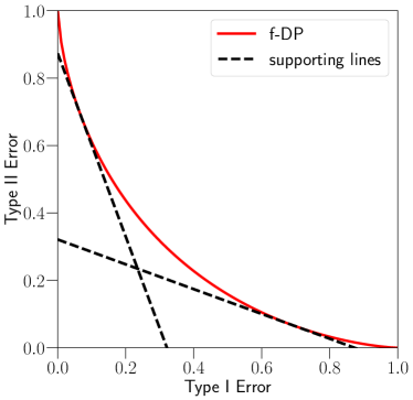
Figure 2.1: An example of a trade-off function and two supporting lines induced by the associated (ε,δ(ε))𝜀𝛿𝜀(\varepsilon,\delta(\varepsilon))-DP guarantees. These lines have slopes e±εsuperscript𝑒plus-or-minus𝜀-e^{\pm\varepsilon}, respectively, and intercepts 1δ1𝛿1-\delta.

Duality to (ε,δ)𝜀𝛿(\varepsilon,\delta)-DP.

The f𝑓f-DP framework has a dual relationship with (ε,δ)𝜀𝛿(\varepsilon,\delta)-DP in the sense that f𝑓f-DP is equivalent to an infinite collection of (ε,δ)𝜀𝛿(\varepsilon,\delta)-DP guarantees via the convex conjugate of f𝑓f. One can view f𝑓f-DP as the primal representation of privacy, and accordingly, its dual representation is the collection of (ε,δ)𝜀𝛿(\varepsilon,\delta)-DP guarantees. In this paper, the Edgeworth approximation addresses f𝑓f-DP from the primal perspective. However, it is also instructive to check the dual presentation. The following propositions introduce how to convert the primal to the dual, and vice versa. Geometrically, each associated (ε,δ)𝜀𝛿(\varepsilon,\delta)-DP guarantee defines two symmetric supporting linear functions to f𝑓f (assuming f𝑓f is symmetric). See Figure 2.1.

Proposition 2.3 (Primal to Dual).

For a symmetric trade-off function f𝑓f, let f::superscript𝑓f^{*}:\mathbb{R}\rightarrow\mathbb{R} be its convex conjugate function f(y)=sup0x1yxf(x)superscript𝑓𝑦subscriptsupremum0𝑥1𝑦𝑥𝑓𝑥f^{*}(y)=\sup_{0\leq x\leq 1}yx-f(x). A mechanism is f𝑓f-DP if and only if it is (ε,δ(ε))𝜀𝛿𝜀(\varepsilon,\delta(\varepsilon))-DP for all ε0𝜀0\varepsilon\geq 0 with δ(ε)=1+f(eε)𝛿𝜀1superscript𝑓superscript𝑒𝜀\delta(\varepsilon)=1+f^{*}(-e^{\varepsilon}).

Proposition 2.4 (Dual to Primal).

Let I𝐼I be an arbitrary index set such that each iI𝑖𝐼i\in I is associated with εi[0,)subscript𝜀𝑖0\varepsilon_{i}\in[0,\infty) and δi[0,1]subscript𝛿𝑖01\delta_{i}\in[0,1]. A mechanism is (εi,δi)subscript𝜀𝑖subscript𝛿𝑖(\varepsilon_{i},\delta_{i})-DP for all iI𝑖𝐼i\in I if and only if it is f𝑓f-DP with f=supiIfεi,δi𝑓subscriptsupremum𝑖𝐼subscript𝑓subscript𝜀𝑖subscript𝛿𝑖f=\sup_{i\in I}f_{\varepsilon_{i},\delta_{i}}, where fε,δ(α)=max{0,1δeεα,eε(1δα)}subscript𝑓𝜀𝛿𝛼01𝛿superscript𝑒𝜀𝛼superscript𝑒𝜀1𝛿𝛼f_{\varepsilon,\delta}(\alpha)=\max\left\{0,1-\delta-e^{\varepsilon}\alpha,e^{-\varepsilon}(1-\delta-\alpha)\right\} is the trade-off function corresponding to (ϵ,δ)italic-ϵ𝛿(\epsilon,\delta)-DP.

Next, we introduce how f𝑓f-DP guarantees degrade under composition. With regard to composition, SGD offers an important benchmark for testing a privacy definition. As a popular optimizer for training deep neural networks, SGD outputs a series of models that are generated from the composition of many gradient descent updates. Furthermore, each step of update is computed from a subsampled mini-batch of data points. While composition degrades the privacy, in contrast, subsampling amplifies the privacy as individuals uncollected in the mini-batch have perfect privacy. Quantifying these two operations under the f𝑓f-DP framework is crucial for analyzing the privacy guarantee of deep learning models trained by noisy SGD.

Composition.

Let f1=T(P1,Q1)subscript𝑓1𝑇subscript𝑃1subscript𝑄1f_{1}=T(P_{1},Q_{1}) and f2=T(P2,Q2)subscript𝑓2𝑇subscript𝑃2subscript𝑄2f_{2}=T(P_{2},Q_{2}), [DRS19] defines a binary operator tensor-product\otimes on trade-off functions such that f1f2=T(P1×P2,Q1×Q2)tensor-productsubscript𝑓1subscript𝑓2𝑇subscript𝑃1subscript𝑃2subscript𝑄1subscript𝑄2f_{1}\otimes f_{2}=T(P_{1}\times P_{2},Q_{1}\times Q_{2}), where P1×P2subscript𝑃1subscript𝑃2P_{1}\times P_{2} is the distribution product. This operator is commutative and associative. The composition primitive refers to an algorithm M𝑀M that consists of n𝑛n algorithms M1,,Mnsubscript𝑀1subscript𝑀𝑛M_{1},\ldots,M_{n}, where Misubscript𝑀𝑖M_{i} observes both the input dataset and output from all previous algorithms111In this paper, n𝑛n denotes the number of private algorithms under composition, as opposed to the number of individuals in the dataset. This is to be consistent with the literature on central limit theorems.. In [DRS19], it is shown that if Misubscript𝑀𝑖M_{i} is fisubscript𝑓𝑖f_{i}-DP for 1in1𝑖𝑛1\leq i\leq n, then the composed algorithm M𝑀M is f1fntensor-productsubscript𝑓1subscript𝑓𝑛f_{1}\otimes\cdots\otimes f_{n}-DP. The authors further identify a central limit theorem-type phenomenon of the overall privacy loss under composition. Loosely speaking, the privacy guarantee asymptotically converges to GDP in the sense that f1fnGμtensor-productsubscript𝑓1subscript𝑓𝑛subscript𝐺𝜇f_{1}\otimes\cdots\otimes f_{n}\rightarrow G_{\mu} as n𝑛n\rightarrow\infty under certain conditions. The privacy parameter μ𝜇\mu depends on the trade-off functions f1,,fnsubscript𝑓1subscript𝑓𝑛f_{1},\ldots,f_{n}.

Subsampling.

Consider the operator SamplepsubscriptSample𝑝\texttt{Sample}_{p} that includes each individual in the dataset with probability p𝑝p independently. Let MSamplep𝑀subscriptSample𝑝M\circ\texttt{Sample}_{p} denote the algorithm where M𝑀M is applied to the subsampled dataset. In the subsampling theorem for f𝑓f-DP, [DRS19] proves that if M𝑀M is f𝑓f-DP, then MSamplep(S)𝑀subscriptSample𝑝𝑆M\circ\texttt{Sample}_{p}(S) is f~~𝑓\tilde{f}-DP if f~fp~𝑓subscript𝑓𝑝\tilde{f}\leq f_{p} and f~fp1~𝑓superscriptsubscript𝑓𝑝1\tilde{f}\leq f_{p}^{-1}, where fp=pf+(1p)Idsubscript𝑓𝑝𝑝𝑓1𝑝Idf_{p}=pf+(1-p)\text{Id}. As such, we can take f~=min{fp,fp1}~𝑓subscript𝑓𝑝superscriptsubscript𝑓𝑝1\tilde{f}=\min\{f_{p},f_{p}^{-1}\}, which is not convex in general however. This issue can be resolved by using min{fp,fp1}\min\{f_{p},f_{p}^{-1}\}^{**} in place of min{fp,fp1}subscript𝑓𝑝superscriptsubscript𝑓𝑝1\min\{f_{p},f_{p}^{-1}\}, where fsuperscript𝑓absentf^{**} denotes the double conjugate of f𝑓f. Indeed, [DRS19] shows that the subsampled algorithm is min{fp,fp1}\min\left\{f_{p},f_{p}^{-1}\right\}^{**}-DP.

Noisy SGD.

Let Mσsubscript𝑀𝜎M_{\sigma} denote the noisy gradient descent update, where σ𝜎\sigma is the scale of the Gaussian noise added to the gradient. The noisy SGD update can essentially be represented as Mσsamplepsubscript𝑀𝜎subscriptsample𝑝M_{\sigma}\circ\text{sample}_{p}. Exploiting the above results for composition and subsampling, [BDLS19] shows that MσSamplepsubscript𝑀𝜎subscriptSample𝑝M_{\sigma}\circ\text{Sample}_{p} is min{h,h1}superscript1\min\{h,h^{-1}\}-DP, where h=pG1/σ+(1p)Id𝑝subscript𝐺1𝜎1𝑝Idh=pG_{1/\sigma}+(1-p)\text{Id}. Recognizing that noisy SGD with n𝑛n iterations is the n𝑛n-fold composition of MσSamplep(S)subscript𝑀𝜎subscriptSample𝑝𝑆M_{\sigma}\circ\text{Sample}_{p}(S), the overall privacy lower bound is min{g,g1}𝑔superscript𝑔1\min\{g,g^{-1}\}-DP, where g=hn=(pG1/σ+(1p)Id)n𝑔superscripttensor-productabsent𝑛superscript𝑝subscript𝐺1𝜎1𝑝Idtensor-productabsent𝑛g=h^{\otimes n}=(pG_{1/\sigma}+(1-p)\text{Id})^{\otimes n}. To evaluate the composition bound, [BDLS19] uses a central limit theorem-type result in the asymptotic regime where pn𝑝𝑛p\sqrt{n} converges to a positive constant as n𝑛n\rightarrow\infty: in this regime, one can show gGpn(e1/σ21)𝑔subscript𝐺𝑝𝑛superscript𝑒1superscript𝜎21g\rightarrow G_{p\sqrt{n(e^{1/\sigma^{2}}-1)}} and consequently min{g,g1}Gpn(e1/σ21)\min\left\{g,g^{-1}\right\}^{**}\rightarrow G_{p\sqrt{n(e^{1/\sigma^{2}}-1)}} as well.

3 Edgeworth Approximation

In this section, we introduce the Edgeworth expansion-based approach to computing the privacy bound under composition. The development of this approach builds on [DRS19], with two crucial modifications.

Consider the hypothesis testing problem H0:𝒙P1××Pn:subscript𝐻0similar-to𝒙subscript𝑃1subscript𝑃𝑛H_{0}:\bm{x}\sim P_{1}\times\cdots\times P_{n} vs H1:𝒙Q1××Qn:subscript𝐻1similar-to𝒙subscript𝑄1subscript𝑄𝑛H_{1}:\bm{x}\sim Q_{1}\times\cdots\times Q_{n}. Let P𝑃P denote the distribution P1××Pnsubscript𝑃1subscript𝑃𝑛P_{1}\times\cdots\times P_{n}, and pi()subscript𝑝𝑖p_{i}(\cdot) denote the probability density functions of Pisubscript𝑃𝑖P_{i}. Correspondingly, we define Q𝑄Q and qisubscript𝑞𝑖q_{i} in the same way. Letting Li()=logqi()pi()subscript𝐿𝑖subscript𝑞𝑖subscript𝑝𝑖\displaystyle L_{i}(\cdot)=\log\frac{q_{i}(\cdot)}{p_{i}(\cdot)}, the likelihood ratio test statistic is given by Tn(𝒙)=logi=1nqi(xi)i=1npi(xi)=i=1nLi(xi).subscript𝑇𝑛𝒙superscriptsubscriptproduct𝑖1𝑛subscript𝑞𝑖subscript𝑥𝑖superscriptsubscriptproduct𝑖1𝑛subscript𝑝𝑖subscript𝑥𝑖superscriptsubscript𝑖1𝑛subscript𝐿𝑖subscript𝑥𝑖\displaystyle T_{n}(\bm{x})=\log\dfrac{\prod_{i=1}^{n}q_{i}(x_{i})}{\prod_{i=1}^{n}p_{i}(x_{i})}=\sum_{i=1}^{n}L_{i}(x_{i}). The Neyman–Pearson lemma states that the most powerful test at a given significance level α𝛼\alpha must be a thresholding function of Tn(𝒙)subscript𝑇𝑛𝒙T_{n}(\bm{x}). As a result, the optimal rejection rule would reject H0subscript𝐻0H_{0} if Tn(𝒙)>ηsubscript𝑇𝑛𝒙𝜂T_{n}(\bm{x})>\eta, where η𝜂\eta is determined by α𝛼\alpha. An equivalent rule is to apply thresholding to the standardized statistic: H0subscript𝐻0H_{0} is rejected if

Tn(𝒙)𝔼P[Tn(𝒙)]𝕍arP[Tn(𝒙)]>h(α),subscript𝑇𝑛𝒙subscript𝔼𝑃delimited-[]subscript𝑇𝑛𝒙𝕍subscriptar𝑃delimited-[]subscript𝑇𝑛𝒙𝛼\frac{T_{n}(\bm{x})-\mathbb{E}_{P}[T_{n}(\bm{x})]}{\sqrt{\mathbb{V}\text{ar}_{P}[T_{n}(\bm{x})]}}>h(\alpha), (3.1)

where the threshold hh is determined by α𝛼\alpha.

In the sequel, for notational simplicity we shall use Tnsubscript𝑇𝑛T_{n} to denote Tn(𝒙)subscript𝑇𝑛𝒙T_{n}(\bm{x}), though it is a function of 𝒙𝒙\bm{x}. Let Fn()subscript𝐹𝑛F_{n}(\cdot) be the CDF of Tn𝔼P[Tn]𝕍arP[Tn]subscript𝑇𝑛subscript𝔼𝑃delimited-[]subscript𝑇𝑛𝕍subscriptar𝑃delimited-[]subscript𝑇𝑛\dfrac{T_{n}-\mathbb{E}_{P}[T_{n}]}{\sqrt{\mathbb{V}\text{ar}_{P}[T_{n}]}} when 𝒙𝒙\bm{x} is drawn from P𝑃P. That is, Fn(h)=p(Tn𝔼P[Tn]𝕍arP[Tn]h).subscript𝐹𝑛subscript𝑝subscript𝑇𝑛subscript𝔼𝑃delimited-[]subscript𝑇𝑛𝕍subscriptar𝑃delimited-[]subscript𝑇𝑛F_{n}(h)=\operatorname{\mathbb{P}}_{p}\left(\frac{T_{n}-\mathbb{E}_{P}[T_{n}]}{\sqrt{\mathbb{V}\text{ar}_{P}[T_{n}]}}\leq h\right). By the Lyapunov CLT, the standardized statistic Tn𝔼P[Tn]𝕍arP[Tn]subscript𝑇𝑛subscript𝔼𝑃delimited-[]subscript𝑇𝑛𝕍subscriptar𝑃delimited-[]subscript𝑇𝑛\frac{T_{n}-\mathbb{E}_{P}[T_{n}]}{\sqrt{\mathbb{V}\text{ar}_{P}[T_{n}]}} converges in distribution to the standard normal random variable. In other words, it holds that

Tn𝔼P[Tn]𝕍arP[Tn]𝑑𝒩(0,1),Fn()Φ()formulae-sequence𝑑subscript𝑇𝑛subscript𝔼𝑃delimited-[]subscript𝑇𝑛𝕍subscriptar𝑃delimited-[]subscript𝑇𝑛𝒩01subscript𝐹𝑛Φ\frac{T_{n}-\mathbb{E}_{P}[T_{n}]}{\sqrt{\mathbb{V}\text{ar}_{P}[T_{n}]}}\xrightarrow{d}\mathcal{N}(0,1),\hskip 15.0ptF_{n}(\cdot)\rightarrow\Phi(\cdot)

as n𝑛n\rightarrow\infty. Likewise, we write F~n(h)=Q(Tn𝔼Q[Tn]𝕍arQ[Tn]h)subscript~𝐹𝑛subscript𝑄subscript𝑇𝑛subscript𝔼𝑄delimited-[]subscript𝑇𝑛𝕍subscriptar𝑄delimited-[]subscript𝑇𝑛\widetilde{F}_{n}(h)=\operatorname{\mathbb{P}}_{Q}\left(\frac{T_{n}-\mathbb{E}_{Q}[T_{n}]}{\sqrt{\mathbb{V}\text{ar}_{Q}[T_{n}]}}\leq h\right) with 𝒙Qsimilar-to𝒙𝑄\bm{x}\sim Q and get

Tn𝔼Q[Tn]𝕍arQ[Tn]𝑑𝒩(0,1),F~n()Φ().formulae-sequence𝑑subscript𝑇𝑛subscript𝔼𝑄delimited-[]subscript𝑇𝑛𝕍subscriptar𝑄delimited-[]subscript𝑇𝑛𝒩01subscript~𝐹𝑛Φ\frac{T_{n}-\mathbb{E}_{Q}[T_{n}]}{\sqrt{\mathbb{V}\text{ar}_{Q}[T_{n}]}}\xrightarrow{d}\mathcal{N}(0,1),\hskip 15.0pt\widetilde{F}_{n}(\cdot)\rightarrow\Phi(\cdot).

With these notations in place, one can write the type I error of the rejection rule (3.1) as

α=P(Tn𝔼P[Tn]𝕍arP[Tn]>h)=1Fn(h).𝛼subscript𝑃subscript𝑇𝑛subscript𝔼𝑃delimited-[]subscript𝑇𝑛𝕍subscriptar𝑃delimited-[]subscript𝑇𝑛1subscript𝐹𝑛\alpha=\operatorname{\mathbb{P}}_{P}\bigg{(}\frac{T_{n}-\mathbb{E}_{P}[T_{n}]}{\sqrt{\mathbb{V}\text{ar}_{P}[T_{n}]}}>h\bigg{)}=1-F_{n}(h). (3.2)

The type II error of this test, which is f(α)𝑓𝛼f(\alpha) by definition, is given by

f(α)𝑓𝛼\displaystyle f(\alpha) =\displaystyle= Q(Tn𝔼P[Tn]𝕍arP[Tn]h)subscript𝑄subscript𝑇𝑛subscript𝔼𝑃delimited-[]subscript𝑇𝑛𝕍subscriptar𝑃delimited-[]subscript𝑇𝑛\displaystyle\operatorname{\mathbb{P}}_{Q}\bigg{(}\frac{T_{n}-\mathbb{E}_{P}[T_{n}]}{\sqrt{\mathbb{V}\text{ar}_{P}[T_{n}]}}\leq h\bigg{)}
=\displaystyle= Q(Tn𝔼Q[Tn]𝕍arP[Tn]h𝔼Q[Tn]𝔼P[Tn]𝕍arP[Tn]).subscript𝑄subscript𝑇𝑛subscript𝔼𝑄delimited-[]subscript𝑇𝑛𝕍subscriptar𝑃delimited-[]subscript𝑇𝑛subscript𝔼𝑄delimited-[]subscript𝑇𝑛subscript𝔼𝑃delimited-[]subscript𝑇𝑛𝕍subscriptar𝑃delimited-[]subscript𝑇𝑛\displaystyle\operatorname{\mathbb{P}}_{Q}\bigg{(}\frac{T_{n}-\mathbb{E}_{Q}[T_{n}]}{\sqrt{\mathbb{V}\text{ar}_{P}[T_{n}]}}\leq h-\frac{\mathbb{E}_{Q}[T_{n}]-\mathbb{E}_{P}[T_{n}]}{\sqrt{\mathbb{V}\text{ar}_{P}[T_{n}]}}\bigg{)}.

In [DRS19], the authors assume that f𝑓f is symmetric and therefore derive the identity 𝕍arQ(Tn)=𝕍arP(Tn)𝕍subscriptar𝑄subscript𝑇𝑛𝕍subscriptar𝑃subscript𝑇𝑛\mathbb{V}\text{ar}_{Q}(T_{n})=\mathbb{V}\text{ar}_{P}(T_{n}). As a consequence, f(α)𝑓𝛼f(\alpha) can be written as F~n(hμn)subscript~𝐹𝑛subscript𝜇𝑛\widetilde{F}_{n}(h-\mu_{n}), where μn=(𝔼Q[Tn]𝔼P[Tn])/𝕍arQ[Tn]subscript𝜇𝑛subscript𝔼𝑄delimited-[]subscript𝑇𝑛subscript𝔼𝑃delimited-[]subscript𝑇𝑛𝕍subscriptar𝑄delimited-[]subscript𝑇𝑛\mu_{n}=(\mathbb{E}_{Q}[T_{n}]-\mathbb{E}_{P}[T_{n}])/\sqrt{\mathbb{V}\text{ar}_{Q}[T_{n}]}. Taken together, the equations above give rise to f(α)=F~n(Fn1(1α)μn)𝑓𝛼subscript~𝐹𝑛subscriptsuperscript𝐹1𝑛1𝛼subscript𝜇𝑛f(\alpha)=\widetilde{F}_{n}(F^{-1}_{n}(1-\alpha)-\mu_{n}). Leveraging this expression of f𝑓f, [DRS19] proves a CLT-type asymptotic convergence result under certain conditions:

f(α)Gμ(α)=Φ(Φ1(1α)μ)𝑓𝛼subscript𝐺𝜇𝛼ΦsuperscriptΦ11𝛼𝜇f(\alpha)\rightarrow G_{\mu}(\alpha)=\Phi(\Phi^{-1}(1-\alpha)-\mu) (3.3)

as n𝑛n\rightarrow\infty, where μ𝜇\mu is the limit of μnsubscript𝜇𝑛\mu_{n}.

Now, we discard the symmetry assumption and just rewrite

f(α)=𝑓𝛼absent\displaystyle f(\alpha)= Q(Tn𝔼P[Tn]𝕍arP[Tn]h)subscript𝑄subscript𝑇𝑛subscript𝔼𝑃delimited-[]subscript𝑇𝑛𝕍subscriptar𝑃delimited-[]subscript𝑇𝑛\displaystyle\hskip 3.0pt\operatorname{\mathbb{P}}_{Q}\bigg{(}\frac{T_{n}-\mathbb{E}_{P}[T_{n}]}{\sqrt{\mathbb{V}\text{ar}_{P}[T_{n}]}}\leq h\bigg{)} (3.4)
=\displaystyle= Q(Tn𝔼Q[Tn]𝕍arP[Tn]h𝔼Q[Tn]𝔼P[Tn]𝕍arP[Tn])subscript𝑄subscript𝑇𝑛subscript𝔼𝑄delimited-[]subscript𝑇𝑛𝕍subscriptar𝑃delimited-[]subscript𝑇𝑛subscript𝔼𝑄delimited-[]subscript𝑇𝑛subscript𝔼𝑃delimited-[]subscript𝑇𝑛𝕍subscriptar𝑃delimited-[]subscript𝑇𝑛\displaystyle\hskip 3.0pt\operatorname{\mathbb{P}}_{Q}\bigg{(}\frac{T_{n}-\mathbb{E}_{Q}[T_{n}]}{\sqrt{\mathbb{V}\text{ar}_{P}[T_{n}]}}\leq h-\frac{\mathbb{E}_{Q}[T_{n}]-\mathbb{E}_{P}[T_{n}]}{\sqrt{\mathbb{V}\text{ar}_{P}[T_{n}]}}\bigg{)}
=\displaystyle= Q(Tn𝔼Q[Tn]𝕍arQ[Tn][h𝔼Q[Tn]𝔼P[Tn]𝕍arP[Tn]]𝕍arP[Tn]𝕍arQ[Tn])subscript𝑄subscript𝑇𝑛subscript𝔼𝑄delimited-[]subscript𝑇𝑛𝕍subscriptar𝑄delimited-[]subscript𝑇𝑛delimited-[]subscript𝔼𝑄delimited-[]subscript𝑇𝑛subscript𝔼𝑃delimited-[]subscript𝑇𝑛𝕍subscriptar𝑃delimited-[]subscript𝑇𝑛𝕍subscriptar𝑃delimited-[]subscript𝑇𝑛𝕍subscriptar𝑄delimited-[]subscript𝑇𝑛\displaystyle\hskip 3.0pt\operatorname{\mathbb{P}}_{Q}\bigg{(}\frac{T_{n}-\mathbb{E}_{Q}[T_{n}]}{\sqrt{\mathbb{V}\text{ar}_{Q}[T_{n}]}}\leq\bigg{[}h-\frac{\mathbb{E}_{Q}[T_{n}]-\mathbb{E}_{P}[T_{n}]}{\sqrt{\mathbb{V}\text{ar}_{P}[T_{n}]}}\bigg{]}\sqrt{\frac{\mathbb{V}\text{ar}_{P}[T_{n}]}{\mathbb{V}\text{ar}_{Q}[T_{n}]}}\bigg{)}
=\displaystyle= F~n((hμn)𝕍arP[Tn]𝕍arQ[Tn]).subscript~𝐹𝑛subscript𝜇𝑛𝕍subscriptar𝑃delimited-[]subscript𝑇𝑛𝕍subscriptar𝑄delimited-[]subscript𝑇𝑛\displaystyle\hskip 3.0pt\widetilde{F}_{n}\bigg{(}(h-\mu_{n})\sqrt{\frac{\mathbb{V}\text{ar}_{P}[T_{n}]}{\mathbb{V}\text{ar}_{Q}[T_{n}]}}\bigg{)}.

Plugging Equation 3.2 into 3.4, we obtain

f(α)=F~n((Fn1(1α)μn)𝕍arP[Tn]𝕍arQ[Tn]).𝑓𝛼subscript~𝐹𝑛subscriptsuperscript𝐹1𝑛1𝛼subscript𝜇𝑛𝕍subscriptar𝑃delimited-[]subscript𝑇𝑛𝕍subscriptar𝑄delimited-[]subscript𝑇𝑛f(\alpha)=\widetilde{F}_{n}\bigg{(}\left(F^{-1}_{n}(1-\alpha)-\mu_{n}\right)\sqrt{\frac{\mathbb{V}\text{ar}_{P}[T_{n}]}{\mathbb{V}\text{ar}_{Q}[T_{n}]}}\bigg{)}. (3.5)

In the special case f𝑓f is symmetric, the factor 𝕍arP[Tn]𝕍arQ[Tn]𝕍subscriptar𝑃delimited-[]subscript𝑇𝑛𝕍subscriptar𝑄delimited-[]subscript𝑇𝑛\sqrt{\frac{\mathbb{V}\text{ar}_{P}[T_{n}]}{\mathbb{V}\text{ar}_{Q}[T_{n}]}} is equal to one and we recover the result in [DRS19].

To obtain the composition bound, the exact computing of Equation 3.5 is not trivial. In Section 5.1 we present a numerical method to compute it directly; however, this method is computationally daunting and could not scale to a large number of compositions. The CLT estimator (Equation 3.3) can be computed quickly, however it can be loose for a small or moderate number of compositions. More importantly, in practice, we observe that the CLT estimator does not handle the composition of asymmetric trade-off functions well. To address these issues, we propose a two-sided approximation method, where the Edgeworth expansion is applied to both Fnsubscript𝐹𝑛F_{n} and F~nsubscript~𝐹𝑛\widetilde{F}_{n} in Equation 3.5. Our method leads to more accurate description of f(α)𝑓𝛼f(\alpha), as justified in Section 5.

3.1 Technical Details

In Equation 3.5, we need to evaluate F~nsubscript~𝐹𝑛\widetilde{F}_{n} and Fn1superscriptsubscript𝐹𝑛1F_{n}^{-1}. Our methods for addressing each of them are described below.

Approximate F~nsubscript~𝐹𝑛\widetilde{F}_{n}.

Assume 𝒙Qsimilar-to𝒙𝑄\bm{x}\sim Q. Denote

XQ=Tn𝔼Q[Tn]𝕍arQ(Tn)=i=1n(Liμi)i=1nσi2,subscript𝑋𝑄subscript𝑇𝑛subscript𝔼𝑄delimited-[]subscript𝑇𝑛𝕍subscriptar𝑄subscript𝑇𝑛superscriptsubscript𝑖1𝑛subscript𝐿𝑖subscript𝜇𝑖superscriptsubscript𝑖1𝑛subscriptsuperscript𝜎2𝑖X_{Q}=\frac{T_{n}-\mathbb{E}_{Q}[T_{n}]}{\sqrt{\mathbb{V}\text{ar}_{Q}(T_{n})}}=\frac{\sum_{i=1}^{n}(L_{i}-\mu_{i})}{\sqrt{\sum_{i=1}^{n}\sigma^{2}_{i}}}, (3.6)

where μisubscript𝜇𝑖\mu_{i} and σi2superscriptsubscript𝜎𝑖2\sigma_{i}^{2} are the mean and variance of Lisubscript𝐿𝑖L_{i} under distribution Qisubscript𝑄𝑖Q_{i}. Recall F~nsubscript~𝐹𝑛\widetilde{F}_{n} is the CDF of XQsubscript𝑋𝑄X_{Q}, and we can apply the Edgeworth expansion to approximate F~nsubscript~𝐹𝑛\widetilde{F}_{n} directly, following the techniques introduced in [Hal13]. It provides a family of series that approximate F~nsubscript~𝐹𝑛\widetilde{F}_{n} in terms of the cumulants of XQsubscript𝑋𝑄X_{Q}, which can be derived from the cumulants of Lisubscript𝐿𝑖L_{i}s under distribution Qisubscript𝑄𝑖Q_{i}s. See Definition 3.1 for the notion of cumulant and Appendix B for how to compute them.

Definition 3.1.

For a random variable X𝑋X, let K(t)𝐾𝑡K(t) be the natural logarithm of the moment-generating function of X𝑋X: K(t)=log𝔼(etX)𝐾𝑡𝔼superscript𝑒𝑡𝑋K(t)=\log\operatorname{\mathbb{E}}\left(e^{tX}\right). The cumulants of X𝑋X, denoted by κ0,,κr,subscript𝜅0subscript𝜅𝑟\kappa_{0},\ldots,\kappa_{r},\ldots for integer r>0𝑟0r>0, are the coefficients in the Taylor expansion of K(t)𝐾𝑡K(t) about the origin: K(t)=log𝔼(etX)=r=0κrtr/r!.𝐾𝑡𝔼superscript𝑒𝑡𝑋superscriptsubscript𝑟0subscript𝜅𝑟superscript𝑡𝑟𝑟K(t)=\log\operatorname{\mathbb{E}}\left(e^{tX}\right)=\sum_{r=0}^{\infty}\kappa_{r}t^{r}/r!.

The key idea of the Edgeworth approximation is to write the characteristic function of the distribution of XQsubscript𝑋𝑄X_{Q} as the following form:

χn(t)=(1+j=1Pj(it)nj/2)exp(t2/2),subscript𝜒𝑛𝑡1superscriptsubscript𝑗1subscript𝑃𝑗𝑖𝑡superscript𝑛𝑗2superscript𝑡22\chi_{n}(t)=\bigg{(}1+\sum_{j=1}^{\infty}{\frac{P_{j}(it)}{n^{j/2}}}\bigg{)}\exp(-t^{2}/2),

where Pjsubscript𝑃𝑗P_{j} is a polynomial with degree 3j3𝑗3j, and then truncate the series up to a fixed number of terms. The corresponding CDF approximation is obtained by the inverse Fourier transform of the truncated series. The Edgeworth approximation of degree j𝑗j amounts to truncating the above series up to terms of order nj2superscript𝑛𝑗2n^{-\frac{j}{2}}.

Let κ~r(Li)subscript~𝜅𝑟subscript𝐿𝑖\tilde{\kappa}_{r}(L_{i}) be the r𝑟r-th cumulant of Lisubscript𝐿𝑖L_{i} under Qisubscript𝑄𝑖Q_{i}, and 𝜿~r=i=1nκ~r(Li)subscriptbold-~𝜿𝑟superscriptsubscript𝑖1𝑛subscript~𝜅𝑟subscript𝐿𝑖\bm{\tilde{\kappa}}_{r}=\sum_{i=1}^{n}\tilde{\kappa}_{r}(L_{i}). Let σn=i=1nσi2subscript𝜎𝑛superscriptsubscript𝑖1𝑛subscriptsuperscript𝜎2𝑖\sigma_{n}=\sqrt{\sum_{i=1}^{n}\sigma^{2}_{i}}. Denoted by F~𝙴𝚆(h)subscript~𝐹𝙴𝚆\widetilde{F}_{\mathtt{EW}}(h) 222We note that F~𝙴𝚆(h)subscript~𝐹𝙴𝚆\widetilde{F}_{\mathtt{EW}}(h) is not guaranteed to be a valid CDF in general, however it is a numerical approximation to Fn(h)subscript𝐹𝑛F_{n}(h) with improved error bounds compared to the CLT approximation., the degree-222 Edgeworth approximation of F~n(h)subscript~𝐹𝑛\widetilde{F}_{n}(h) is given by

F~𝙴𝚆(h)=Φ(h)σn316𝜿~3(h21)ϕ(h)T1subscript~𝐹𝙴𝚆Φsuperscriptsuperscriptsubscript𝜎𝑛316subscriptbold-~𝜿3superscript21italic-ϕsubscript𝑇1\displaystyle\widetilde{F}_{\mathtt{EW}}(h)=\Phi(h)-\overbrace{\sigma_{n}^{-3}\cdot\frac{1}{6}\bm{\tilde{\kappa}}_{3}(h^{2}-1)\phi(h)}^{T_{1}} (3.7)
(σn424𝜿~4(h33h)+σn672𝜿~32(h510h3+15h))ϕ(h)T2.superscriptsuperscriptsubscript𝜎𝑛424subscriptbold-~𝜿4superscript33superscriptsubscript𝜎𝑛672superscriptsubscriptbold-~𝜿32superscript510superscript315italic-ϕsubscript𝑇2\displaystyle-\overbrace{\left(\frac{\sigma_{n}^{-4}}{24}\bm{\tilde{\kappa}}_{4}(h^{3}-3h)+\frac{\sigma_{n}^{-6}}{72}\bm{\tilde{\kappa}}_{3}^{2}(h^{5}-10h^{3}+15h)\right)\phi(h)}^{T_{2}}.

The term T1subscript𝑇1T_{1} is of order n12superscript𝑛12n^{-\frac{1}{2}} and T2subscript𝑇2T_{2} is of order n1superscript𝑛1n^{-1}. See Appendix A for detailed derivations. Our framework covers the CLT approximation introduced in [DRS19]. The CLT approximation is equivalent to the degree-00 Edgeworth approximation, whose approximation error of order n12superscript𝑛12n^{-\frac{1}{2}}.

Approximate Fn1subscriptsuperscript𝐹1𝑛F^{-1}_{n}.

Refer to caption
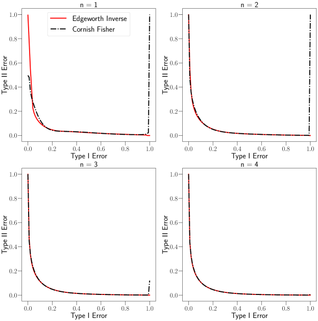
Figure 3.1: Comparison of f(α)𝑓𝛼f(\alpha) obtained when approximating Fn1()subscriptsuperscript𝐹1𝑛F^{-1}_{n}(\cdot) using Method (i) and (ii). The approximation of F~n()subscript~𝐹𝑛\widetilde{F}_{n}(\cdot) is fixed as in Equation 3.7.

In Equation 3.5 we need to compute the Fn1(1α)subscriptsuperscript𝐹1𝑛1𝛼F^{-1}_{n}(1-\alpha). This is the 1α1𝛼1-\alpha quantile of the distribution of Tn(𝒙)𝔼P[Tn(𝒙)]𝕍arP[Tn(𝒙)]subscript𝑇𝑛𝒙subscript𝔼𝑃delimited-[]subscript𝑇𝑛𝒙𝕍subscriptar𝑃delimited-[]subscript𝑇𝑛𝒙\frac{T_{n}(\bm{x})-\mathbb{E}_{P}[T_{n}(\bm{x})]}{\sqrt{\mathbb{V}\text{ar}_{P}[T_{n}(\bm{x})]}}, where 𝒙𝒙\bm{x} is P𝑃P distributed. We consider two approaches to deal with it.

Method (i): First compute the degree-222 Edgeworth approximation F𝙴𝚆()subscript𝐹𝙴𝚆F_{\mathtt{EW}}(\cdot) of Fn()subscript𝐹𝑛F_{n}(\cdot):

F𝙴𝚆(h)=subscript𝐹𝙴𝚆absent\displaystyle F_{\mathtt{EW}}(h)= Φ(h)σn316𝜿3(h21)ϕ(h)Φsuperscriptsubscript𝜎𝑛316subscript𝜿3superscript21italic-ϕ\displaystyle\Phi(h)-\sigma_{n}^{-3}\cdot\frac{1}{6}\bm{\kappa}_{3}(h^{2}-1)\phi(h) (3.8)
σn4124𝜿4(h33h)ϕ(h)superscriptsubscript𝜎𝑛4124subscript𝜿4superscript33italic-ϕ\displaystyle-\sigma_{n}^{-4}\cdot\frac{1}{24}\bm{\kappa}_{4}(h^{3}-3h)\phi(h)
σn6172𝜿32(h510h3+15h)ϕ(h),superscriptsubscript𝜎𝑛6172superscriptsubscript𝜿32superscript510superscript315italic-ϕ\displaystyle-\sigma_{n}^{-6}\cdot\frac{1}{72}\bm{\kappa}_{3}^{2}(h^{5}-10h^{3}+15h)\phi(h),

where 𝜿r=i=1nκr(Li)subscript𝜿𝑟superscriptsubscript𝑖1𝑛subscript𝜅𝑟subscript𝐿𝑖\bm{\kappa}_{r}=\sum_{i=1}^{n}\kappa_{r}(L_{i}) and κr(Li)subscript𝜅𝑟subscript𝐿𝑖\kappa_{r}(L_{i}) is the r𝑟r-th cumulant of Lisubscript𝐿𝑖L_{i} under Pisubscript𝑃𝑖P_{i}. Next, numerically solve equation F𝙴𝚆(h)1α=0subscript𝐹𝙴𝚆1𝛼0F_{\mathtt{EW}}(h)-1-\alpha=0.

Method (ii): Apply the closely related Cornish-Fisher Expansion [CF38, FC60], an asymptotic expansion used to approximate the quantiles of a probability distribution based on its cumulants, to approximate Fn1()subscriptsuperscript𝐹1𝑛F^{-1}_{n}(\cdot) directly. Let z=Φ1(1α)𝑧superscriptΦ11𝛼z=\Phi^{-1}(1-\alpha) be the 1α1𝛼1-\alpha quantile of the standard normal distribution. The degree-2 Cornish-Fisher approximation of the 1α1𝛼1-\alpha quantile of Tn𝔼P[Tn]𝕍arP(Tn)subscript𝑇𝑛subscript𝔼𝑃delimited-[]subscript𝑇𝑛𝕍subscriptar𝑃subscript𝑇𝑛\frac{T_{n}-\mathbb{E}_{P}[T_{n}]}{\sqrt{\mathbb{V}\text{ar}_{P}(T_{n})}} is given by

Fn1(1α)z+σn316𝜿3(z21)subscriptsuperscript𝐹1𝑛1𝛼𝑧superscriptsubscript𝜎𝑛316subscript𝜿3superscript𝑧21\displaystyle F^{-1}_{n}(1-\alpha)\approx z+\sigma_{n}^{-3}\frac{1}{6}\bm{\kappa}_{3}(z^{2}-1) (3.9)
+σn4124𝜿4(z33z)σn6136𝜿32(2z35z).superscriptsubscript𝜎𝑛4124subscript𝜿4superscript𝑧33𝑧superscriptsubscript𝜎𝑛6136superscriptsubscript𝜿322superscript𝑧35𝑧\displaystyle\hskip 10.0pt+\sigma_{n}^{-4}\frac{1}{24}\bm{\kappa}_{4}(z^{3}-3z)-\sigma_{n}^{-6}\frac{1}{36}\bm{\kappa}_{3}^{2}(2z^{3}-5z).

Both approaches have pros and cons. The Cornish-Fisher approximation has closed form solution, yet Figure 3.1 shows that it is unstable at the boundary when the number of compositions is small. For our experiments in Section 5, we use the numerical inverse approach throughout all the runs.

3.2 Error Analysis

Here we provide an error bound for approximating the overall privacy level f𝑓f using Edgeworth expansion. For simplicity, we assume that f𝑓f is symmetric and the log-likelihood ratios Lisubscript𝐿𝑖L_{i}’s are iid distributed with the common distribution having sufficiently light tails for the convergence of the Edgeworth expansion, under both P𝑃P and Q𝑄Q.

The Edgeworth expansion of degree 2 satisfies both Fn(h)F𝙴𝚆(h)=O(n32)subscript𝐹𝑛subscript𝐹𝙴𝚆𝑂superscript𝑛32F_{n}(h)-F_{\mathtt{EW}}(h)=O(n^{-\frac{3}{2}}) and F~n(h)F~𝙴𝚆(h)=O(n32)subscript~𝐹𝑛subscript~𝐹𝙴𝚆𝑂superscript𝑛32\widetilde{F}_{n}(h)-\widetilde{F}_{\mathtt{EW}}(h)=O(n^{-\frac{3}{2}}). Conversely, the inverse satisfies Fn1(α)F𝙴𝚆1(α)=O(n32)superscriptsubscript𝐹𝑛1𝛼superscriptsubscript𝐹𝙴𝚆1𝛼𝑂superscript𝑛32F_{n}^{-1}(\alpha)-F_{\mathtt{EW}}^{-1}(\alpha)=O(n^{-\frac{3}{2}}) and F~n1(α)F~𝙴𝚆1(α)=O(n32)superscriptsubscript~𝐹𝑛1𝛼superscriptsubscript~𝐹𝙴𝚆1𝛼𝑂superscript𝑛32\widetilde{F}_{n}^{-1}(\alpha)-\widetilde{F}_{\mathtt{EW}}^{-1}(\alpha)=O(n^{-\frac{3}{2}}) for α𝛼\alpha that is bounded away from 0 and 1. Making use of these approximation bounds, we get

f𝙴𝚆(α)subscript𝑓𝙴𝚆𝛼\displaystyle f_{\mathtt{EW}}(\alpha) =F~𝙴𝚆(F𝙴𝚆1(1α)μ)absentsubscript~𝐹𝙴𝚆subscriptsuperscript𝐹1𝙴𝚆1𝛼𝜇\displaystyle=\tilde{F}_{\mathtt{EW}}(F^{-1}_{\mathtt{EW}}(1-\alpha)-\mu)
=F~𝙴𝚆(Fn1(1α)+O(n32)μ)absentsubscript~𝐹𝙴𝚆subscriptsuperscript𝐹1𝑛1𝛼𝑂superscript𝑛32𝜇\displaystyle=\tilde{F}_{\mathtt{EW}}(F^{-1}_{n}(1-\alpha)+O(n^{-\frac{3}{2}})-\mu)
=F~n(Fn1(1α)+O(n32)μ)+O(n32)absentsubscript~𝐹𝑛subscriptsuperscript𝐹1𝑛1𝛼𝑂superscript𝑛32𝜇𝑂superscript𝑛32\displaystyle=\tilde{F}_{n}(F^{-1}_{n}(1-\alpha)+O(n^{-\frac{3}{2}})-\mu)+O(n^{-\frac{3}{2}})
=f(α)+O(n32).absent𝑓𝛼𝑂superscript𝑛32\displaystyle=f(\alpha)+O(n^{-\frac{3}{2}}).

As a caveat, we remark that the analysis above does not extend the error bound O(n32)𝑂superscript𝑛32O(n^{-\frac{3}{2}}) to a type I error that is close to 0 or 1. The result states that the approximation error of using the Edgeworth expansion quickly tends to 0 at the rate of O(n32)𝑂superscript𝑛32O(n^{-\frac{3}{2}}). This error rate can be improved at the expense of a higher order expansion of the Edgeworth series. For comparison, our analysis can be carried over to show that the approximation error of using CLT is O(n12)𝑂superscript𝑛12O(n^{-\frac{1}{2}}).

3.3 Computational Cost

The computational cost of the Edgeworth approximation can be broken down as follows. We first need to compute the cumulants of Lisubscript𝐿𝑖L_{i} under Pisubscript𝑃𝑖P_{i} and Qisubscript𝑄𝑖Q_{i} up to a certain order, for i=1,,n𝑖1𝑛i=1,\ldots,n. Next, we need to compute F𝙴𝚆1(1α)subscriptsuperscript𝐹1𝙴𝚆1𝛼F^{-1}_{\mathtt{EW}}(1-\alpha). The Cornish-Fisher approximation (Equation 3.9) costs constant time. If we choose to compute the inverse numerically, we need to evaluate Equation 3.8 then solve a one-dimensional root-finding problem. The former has a constant cost, and the latter can be extremely efficiently computed by various types of iterative methods, for which we can consider the cost as constant too. Finally, it costs constant time to evaluate F~𝙴𝚆()subscript~𝐹𝙴𝚆\widetilde{F}_{\mathtt{EW}}(\cdot) using Equation 3.7. Therefore, the only cost that might scale with the number of compositions n𝑛n is the computation of cumulants. However, in many applications including computing the privacy bound for noisy SGD, all the Lisubscript𝐿𝑖L_{i}s are iid distributed. Under such condition, we only need to compute the cumulants once. The total cost is thus a constant independent of n𝑛n. This is verified by the runtime comparison in Section 5.

4 A Two-Parameter Privacy Interpreter

Let M1subscript𝑀1M_{1} and M2subscript𝑀2M_{2} be two private algorithms that are associated with trade-off functions f1subscript𝑓1f_{1} and f2subscript𝑓2f_{2}, respectively. The algorithm M2subscript𝑀2M_{2} will be more private than M1subscript𝑀1M_{1} if f2subscript𝑓2f_{2} upper bounds f1subscript𝑓1f_{1}. For the family of Gaussian differentially private algorithms, this property can be reflected by the parameter μ0𝜇0\mu\geq 0 directly, where a smaller value of μ𝜇\mu manifests a more private algorithm.

Here we provide a two-parameter description (μ,γ)superscript𝜇𝛾(\mu^{*},\gamma) for the Edgeworth approximation, through which the privacy guarantee between two different approximations can be directly compared.

Given an approximation f𝙴𝚆subscript𝑓𝙴𝚆f_{\mathtt{EW}}, let αsuperscript𝛼\alpha^{*} be its fixed point such that f𝙴𝚆(α)=αsubscript𝑓𝙴𝚆superscript𝛼superscript𝛼f_{\mathtt{EW}}(\alpha^{*})=\alpha^{*}. Let μsuperscript𝜇\mu^{*} be the parameter of GDP for which Gμsubscript𝐺superscript𝜇G_{\mu^{*}} admits the same fixed point as f𝙴𝚆subscript𝑓𝙴𝚆f_{\mathtt{EW}}: Gμ(α)=αsubscript𝐺superscript𝜇superscript𝛼superscript𝛼G_{\mu^{*}}(\alpha^{*})=\alpha^{*}. Such μsuperscript𝜇\mu^{*} can be computed in closed form:

μ=Φ1(1α)Φ1(α).superscript𝜇superscriptΦ11superscript𝛼superscriptΦ1superscript𝛼\mu^{*}=\Phi^{-1}(1-\alpha^{*})-\Phi^{-1}(\alpha^{*}).

Let γ=01f𝙴𝚆(α)𝑑α𝛾superscriptsubscript01subscript𝑓𝙴𝚆𝛼differential-d𝛼\gamma=\int_{0}^{1}f_{\mathtt{EW}}(\alpha)d\alpha be the area under the curve of f𝙴𝚆subscript𝑓𝙴𝚆f_{\mathtt{EW}}.

Two symmetric Edgeworth approximations333If f𝑓f is asymmetric, we can always symmetrize it by taking min{f,f1}\min\left\{f,f^{-1}\right\}^{**}. f𝙴𝚆(1)superscriptsubscript𝑓𝙴𝚆1f_{\mathtt{EW}}^{(1)} and f𝙴𝚆(2)superscriptsubscript𝑓𝙴𝚆2f_{\mathtt{EW}}^{(2)} can be compared in the sense that f𝙴𝚆(2)superscriptsubscript𝑓𝙴𝚆2f_{\mathtt{EW}}^{(2)} is more private than f𝙴𝚆(1)superscriptsubscript𝑓𝙴𝚆1f_{\mathtt{EW}}^{(1)} if their associated parameters (μ(1),γ(1))superscriptsuperscript𝜇1superscript𝛾1({\mu^{*}}^{(1)},\gamma^{(1)}) and (μ(2),γ(2))superscriptsuperscript𝜇2superscript𝛾2({\mu^{*}}^{(2)},\gamma^{(2)}) satisfy the following condition:

μ(2)<μ(1)andγ(2)>γ(1).superscriptsuperscript𝜇2expectationsuperscriptsuperscript𝜇1andsuperscript𝛾2superscript𝛾1{\mu^{*}}^{(2)}<{\mu^{*}}^{(1)}\;\text{and}\;\gamma^{(2)}>\gamma^{(1)}.
Refer to caption
Refer to caption
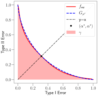
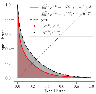
Figure 4.1: Left: An illustration of the (μ,γ)superscript𝜇𝛾(\mu^{*},\gamma) parameterization. Right: f𝙴𝚆(2)subscriptsuperscript𝑓2𝙴𝚆f^{(2)}_{\mathtt{EW}} is more private than f𝙴𝚆(1)subscriptsuperscript𝑓1𝙴𝚆f^{(1)}_{\mathtt{EW}}.

The left panel of Figure 4.1 provides the geometric interpretation of the above parameterization. The Edgeworth approximation f𝙴𝚆subscript𝑓𝙴𝚆f_{\mathtt{EW}}, the CLT approximation Gμsubscript𝐺superscript𝜇G_{\mu^{*}}, and the line y=x𝑦𝑥y=x intersect at the point (α,α)superscript𝛼superscript𝛼(\alpha^{*},\alpha^{*}).

The right panel compares two Edgeworth approximations f𝙴𝚆(1)subscriptsuperscript𝑓1𝙴𝚆f^{(1)}_{\mathtt{EW}} and f𝙴𝚆(2)subscriptsuperscript𝑓2𝙴𝚆f^{(2)}_{\mathtt{EW}}. It is easy to see that in this case f𝙴𝚆(2)subscriptsuperscript𝑓2𝙴𝚆f^{(2)}_{\mathtt{EW}} upper bounds f𝙴𝚆(1)subscriptsuperscript𝑓1𝙴𝚆f^{(1)}_{\mathtt{EW}} and thus it is more private than f𝙴𝚆(1)subscriptsuperscript𝑓1𝙴𝚆f^{(1)}_{\mathtt{EW}}. There are two important properties. First, its intersection with the line y=x𝑦𝑥y=x is further away from the original point than f𝙴𝚆(1)subscriptsuperscript𝑓1𝙴𝚆f^{(1)}_{\mathtt{EW}}. Consider the geometric interpretation shown in the left panel. This implies that μ(2)<μ(1)superscriptsuperscript𝜇2superscriptsuperscript𝜇1{\mu^{*}}^{(2)}<{\mu^{*}}^{(1)}. Second, the approximation f𝙴𝚆(2)subscriptsuperscript𝑓2𝙴𝚆f^{(2)}_{\mathtt{EW}} also has a larger area under the curve than f𝙴𝚆(1)subscriptsuperscript𝑓1𝙴𝚆f^{(1)}_{\mathtt{EW}}, which is essentially γ(2)>γ(1)superscript𝛾2superscript𝛾1\gamma^{(2)}>\gamma^{(1)}.

This parameterization defines a partial order over the set {(μ,γ):μ0, 0γ12}conditional-set𝜇𝛾formulae-sequence𝜇0 0𝛾12\left\{(\mu,\gamma):\;\mu\geq 0,\,0\leq\gamma\leq\frac{1}{2}\right\}444The perfect privacy is attained when the trade-off function is Id(α)=1αId𝛼1𝛼\text{Id}(\alpha)=1-\alpha, whose area under the curve is 1212\frac{1}{2}.. It is also applicable to general trade-off functions.

5 Experiments

In this section, we present numerical experiments to compare the Edgeworth approximation and the CLT approximation. Before we proceed, we introduce a numerical method to directly compute the true composition bound in Section 5.1. This method is not scalable and hence merely serves as a reference for our comparison. We use the Edgeworth approximation of degree 222 for all the experiments. In the sequel, we refer to those methods as Edgeworth, CLT, and Numerical, respectively. All the methods are implemented in Python555The code is available at https://github.com/enosair/gdp-edgeworth. and all the experiments are carried out on a MacBook with 2.5GHz processor and 16GB memory.

5.1 A Numerical Method

Consider the problem of computing fnsuperscript𝑓tensor-productabsent𝑛f^{\otimes n} numerically. We know that we can find P,Q𝑃𝑄P,Q such that f=T(P,Q)𝑓𝑇𝑃𝑄f=T(P,Q) and fn=T(Pn,Qn)superscript𝑓tensor-productabsent𝑛𝑇superscript𝑃𝑛superscript𝑄𝑛f^{\otimes n}=T(P^{n},Q^{n}). However, computing T(Pn,Qn)𝑇superscript𝑃𝑛superscript𝑄𝑛T(P^{n},Q^{n}) directly involves high-dimensional testing, which can be challenging. We show this difficulty can be avoided by going from the primal representation to the dual representation. Let (ε,δk(ε))𝜀subscript𝛿𝑘𝜀(\varepsilon,\delta_{k}(\varepsilon)) be the dual representation associated with fksuperscript𝑓tensor-productabsent𝑘f^{\otimes k}. The method contains three steps to obtain δn(ε)subscript𝛿𝑛𝜀\delta_{n}(\varepsilon) for fnsuperscript𝑓tensor-productabsent𝑛f^{\otimes n}.

  1. 1.

    Convert f𝑓f to δ1(ε)subscript𝛿1𝜀\delta_{1}(\varepsilon). This step can be done implicitly via P𝑃P and Q𝑄Q, see Lemma 5.1.

  2. 2.

    Iteratively compute δk+1(ε)subscript𝛿𝑘1𝜀\delta_{k+1}(\varepsilon) from δk(ε)subscript𝛿𝑘𝜀\delta_{k}(\varepsilon) using Lemma 5.2.

  3. 3.

    Convert δn(ε)subscript𝛿𝑛𝜀\delta_{n}(\varepsilon) to fnsuperscript𝑓tensor-productabsent𝑛f^{\otimes n} using Proposition 2.4.

Next, we explain how to compute δk+1(ε)subscript𝛿𝑘1𝜀\delta_{k+1}(\varepsilon) from δk(ε)subscript𝛿𝑘𝜀\delta_{k}(\varepsilon). First, we need a lemma that relates δ1(ε)subscript𝛿1𝜀\delta_{1}(\varepsilon) with P,Q𝑃𝑄P,Q.

Lemma 5.1.

Suppose f=T(P,Q)𝑓𝑇𝑃𝑄f=T(P,Q) and P,Q𝑃𝑄P,Q have densities p,q𝑝𝑞p,q with respect to a dominating measure μ𝜇\mu. Then the dual representation δ1(ε)=1+f(eε)subscript𝛿1𝜀1superscript𝑓superscripte𝜀\delta_{1}(\varepsilon)=1+f^{*}(-\mathrm{e}^{\varepsilon}) satisfies δ1(ε)=(qeεp)+dμ.subscript𝛿1𝜀subscript𝑞superscripte𝜀𝑝differential-d𝜇\displaystyle\delta_{1}(\varepsilon)=\int(q-\mathrm{e}^{\varepsilon}p)_{+}\mathrm{d}\mu.

Suppose we are given f1=T(P1,Q1),f2=T(P2,Q2)formulae-sequencesubscript𝑓1𝑇subscript𝑃1subscript𝑄1subscript𝑓2𝑇subscript𝑃2subscript𝑄2f_{1}=T(P_{1},Q_{1}),f_{2}=T(P_{2},Q_{2}). Let δ1,δ2subscript𝛿1subscript𝛿2\delta_{1},\delta_{2} and δsubscript𝛿tensor-product\delta_{\otimes} be the dual representations of f1,f2subscript𝑓1subscript𝑓2f_{1},f_{2} and f1f2tensor-productsubscript𝑓1subscript𝑓2f_{1}\otimes f_{2} respectively. The following lemma shows how to evaluate δsubscript𝛿tensor-product\delta_{\otimes} from δ1subscript𝛿1\delta_{1} and δ2subscript𝛿2\delta_{2}. To simplify notations, we assume Pi,Qisubscript𝑃𝑖subscript𝑄𝑖P_{i},Q_{i} are distributions on the real line and have corresponding densities pi,qisubscript𝑝𝑖subscript𝑞𝑖p_{i},q_{i} for i=1,2𝑖12i=1,2 with respect to Lebesgue measure. Generalization to abstract measurable space is straightforward.

Lemma 5.2.

Let L2(y)=logq2(y)p2(y)subscript𝐿2𝑦subscript𝑞2𝑦subscript𝑝2𝑦L_{2}(y)=\log\frac{q_{2}(y)}{p_{2}(y)}. Then δ(ε)=δ1(εL2(y))q2(y)dy.subscript𝛿tensor-product𝜀subscriptsubscript𝛿1𝜀subscript𝐿2𝑦subscript𝑞2𝑦differential-d𝑦\displaystyle\delta_{\otimes}(\varepsilon)=\int_{\mathbb{R}}\delta_{1}\big{(}\varepsilon-L_{2}(y)\big{)}q_{2}(y)\mathrm{d}y.

In particular, it yields a recursive formula to compute fnsuperscript𝑓tensor-productabsent𝑛f^{\otimes n} when f=T(P,Q)𝑓𝑇𝑃𝑄f=T(P,Q). Again we assume P,Q𝑃𝑄P,Q has densities p,q𝑝𝑞p,q on the real line. Let L(x)=logq(x)p(x)𝐿𝑥𝑞𝑥𝑝𝑥L(x)=\log\tfrac{q(x)}{p(x)}. We have

δ0(ε)subscript𝛿0𝜀\displaystyle\delta_{0}(\varepsilon) =max{1eε,0}absent1superscripte𝜀0\displaystyle=\max\{1-\mathrm{e}^{\varepsilon},0\}
δk+1(ε)subscript𝛿𝑘1𝜀\displaystyle\delta_{k+1}(\varepsilon) =δk(εL(x))dxabsentsubscript𝛿𝑘𝜀𝐿𝑥differential-d𝑥\displaystyle=\int\delta_{k}\big{(}\varepsilon-L(x)\big{)}\mathrm{d}x
fn(α)superscript𝑓tensor-productabsent𝑛𝛼\displaystyle f^{\otimes n}(\alpha) =supε1δn(ε)eεα.absentsubscriptsupremum𝜀1subscript𝛿𝑛𝜀superscripte𝜀𝛼\displaystyle=\sup_{\varepsilon\in\mathbb{R}}1-\delta_{n}(\varepsilon)-\mathrm{e}^{\varepsilon}\alpha.

We remark here that if f𝑓f is asymmetric, then the dual involves negative ε𝜀\varepsilon, which is why the conversion to fnsuperscript𝑓tensor-productabsent𝑛f^{\otimes n} involves the whole real line. The proof of the above lemmas is deferred to Appendix D.

In practice, it is more efficient to store δnsubscript𝛿𝑛\delta_{n} in the memory than to perform the computation on the fly, so we need to discretize the domain and store the function value on this grid. Consider an abstract grid {εj}j=1Nsuperscriptsubscriptsubscript𝜀𝑗𝑗1𝑁\{\varepsilon_{j}\}_{j=1}^{N}\subseteq\mathbb{R}, the recursion goes as follows:

δ0(εj)subscript𝛿0subscript𝜀𝑗\displaystyle\delta_{0}(\varepsilon_{j}) =max{1eεj,0},j=1,,Nformulae-sequenceabsent1superscriptesubscript𝜀𝑗0𝑗1𝑁\displaystyle=\max\{1-\mathrm{e}^{\varepsilon_{j}},0\},j=1,\ldots,N
δk+1(εj)subscript𝛿𝑘1subscript𝜀𝑗\displaystyle\delta_{k+1}(\varepsilon_{j}) =δk(εjL(x))dx,j=1,,Nformulae-sequenceabsentsubscript𝛿𝑘subscript𝜀𝑗𝐿𝑥differential-d𝑥𝑗1𝑁\displaystyle=\int\delta_{k}\big{(}\lfloor\varepsilon_{j}-L(x)\rfloor\big{)}\mathrm{d}x,j=1,\ldots,N
fn(α)superscript𝑓tensor-productabsent𝑛𝛼\displaystyle f^{\otimes n}(\alpha) =sup1jN1δn(εj)eεjα.absentsubscriptsupremum1𝑗𝑁1subscript𝛿𝑛subscript𝜀𝑗superscriptesubscript𝜀𝑗𝛼\displaystyle=\sup_{1\leqslant j\leqslant N}1-\delta_{n}(\varepsilon_{j})-\mathrm{e}^{\varepsilon_{j}}\alpha.

where εjL(x)=max{εl:εlεjL(x)}subscript𝜀𝑗𝐿𝑥:subscript𝜀𝑙subscript𝜀𝑙subscript𝜀𝑗𝐿𝑥\lfloor\varepsilon_{j}-L(x)\rfloor=\max\{\varepsilon_{l}:\varepsilon_{l}\leqslant\varepsilon_{j}-L(x)\}. This rounding step can be replaced by an interpolation as well.

The major challenge in making this numerical method practical for computing composition product of trade-off functions is that it is slow in computation as it involves nN𝑛𝑁nN numerical integrations.

5.2 A Moderate Number of Compositions

Section 3 shows that the approximation error of Edgeworth is O(n32)𝑂superscript𝑛32O(n^{-\frac{3}{2}}), and for CLT the error is O(n12)𝑂superscript𝑛12O(n^{-\frac{1}{2}}). We thus expect for small or moderate values of n𝑛n, Edgeworth will produce non-negligible outperformance to CLT. To verify this, we investigate their performance on a toy problem for testing order-n𝑛n compositions of Laplace distributions666 The density function of Lap(θ,b)Lap𝜃𝑏\texttt{Lap}(\theta,b) is 12bexp(|xθ|/b)12𝑏𝑥𝜃𝑏\frac{1}{2b}\exp(-\left|x-\theta\right|/b). : P=Lap(0,1)n𝑃Lapsuperscript01tensor-productabsent𝑛P=\texttt{Lap}(0,1)^{\otimes n} vs Q=Lap(θ,1)n𝑄Lapsuperscript𝜃1tensor-productabsent𝑛Q=\texttt{Lap}(\theta,1)^{\otimes n}.

Refer to caption
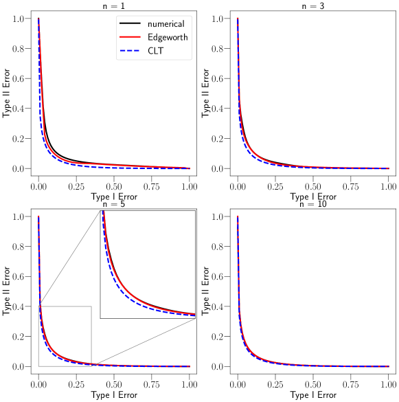
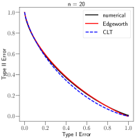
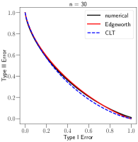
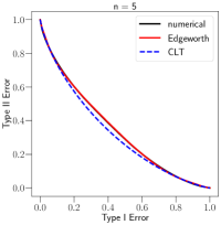
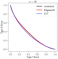
Figure 5.1: The estimated trade-off functions for testing Lap(0,1)nLapsuperscript01tensor-productabsent𝑛\texttt{Lap}(0,1)^{\otimes n} vs Lap(3/n,1)nLapsuperscript3𝑛1tensor-productabsent𝑛\texttt{Lap}(3/\sqrt{n},1)^{\otimes n}.
Refer to caption
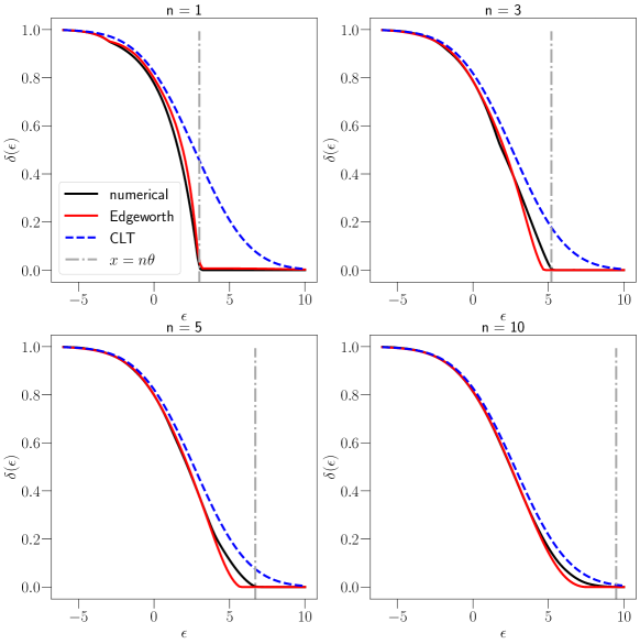
Figure 5.2: The associated (ε,δ(ε))𝜀𝛿𝜀(\varepsilon,\delta(\varepsilon))-DP of the estimated trade-off functions for testing Lap(0,1)nLapsuperscript01tensor-productabsent𝑛\texttt{Lap}(0,1)^{\otimes n} vs Lap(3/n,1)nLapsuperscript3𝑛1tensor-productabsent𝑛\texttt{Lap}(3/\sqrt{n},1)^{\otimes n}.

We let the number of compositions n𝑛n vary from 111 to 101010. Since the privacy guarantee decays as n𝑛n increases and the resulting curves would be very close to the axes, we set θ=3/n𝜃3𝑛\theta=3/\sqrt{n} for the sake of better visibility. Figure 5.1 plots the estimated trade-off functions for four representative cases n=1,3,5,10𝑛13510n=1,3,5,10. For each of the methods, we also compute the associated (ε,δ)𝜀𝛿(\varepsilon,\delta)-DP (see Proposition 2.3) and plot δ𝛿\delta as a function of ε𝜀\varepsilon in Figure 5.2. From both the primal and dual views, Edgeworth coincides better with Numerical in all the cases. When the number of compositions is 10, even though the difference between Edgeworth and CLT is small in the primal visualization (Figure 5.1), the (ε,δ)𝜀𝛿(\varepsilon,\delta) presentation still clearly distinguishes them. In addition, due to the heavy tail of the Laplace distribution, we shall have T({Lap(0,1)}n,{Lap(θ,1)}n)fε,0𝑇superscriptLap01tensor-productabsent𝑛superscriptLap𝜃1tensor-productabsent𝑛subscript𝑓𝜀0T(\left\{\texttt{Lap}(0,1)\right\}^{\otimes n},\left\{\texttt{Lap}(\theta,1)\right\}^{\otimes n})\geq f_{\varepsilon,0} for εnθ𝜀𝑛𝜃\varepsilon\geq n\theta (see Definition 2.4 for the exact form of fε,δsubscript𝑓𝜀𝛿f_{\varepsilon,\delta}). Therefore, the ground truth has the property that δ(ε)=0𝛿𝜀0\delta(\varepsilon)=0 for εnθ𝜀𝑛𝜃\varepsilon\geq n\theta. Figure 5.2 shows that Edgeworth also outperforms CLT for predicting this changing point.

n=2𝑛2n=2 n=4𝑛4n=4 n=6𝑛6n=6 n=8𝑛8n=8 n=10𝑛10n=10
CLT 0.0004 0.0004 0.0004 0.0004 0.0005
Edgeworth 0.2347 0.2341 0.2391 0.2222 0.2234
Numerical 3.6834 7.3361 12.055 16.729 21.3575
Table 1: Runtime for estimating the trade-off function for testing Lap(0,1)nLapsuperscript01tensor-productabsent𝑛\texttt{Lap}(0,1)^{\otimes n} vs Lap(3/n,1)nLapsuperscript3𝑛1tensor-productabsent𝑛\texttt{Lap}(3/\sqrt{n},1)^{\otimes n}.

Table 1 reports the runtime of the above experiment. CLT takes constant computing time at the scale of 1e-4 second. Due to the homogeneity of the component distributions under composition, the runtime of Edgeworth is also invariant of the composition number, which is at the scale of 0.1 second. Numerical is computationally heavy. Its runtime is much larger and grows linearly as the number of compositions.
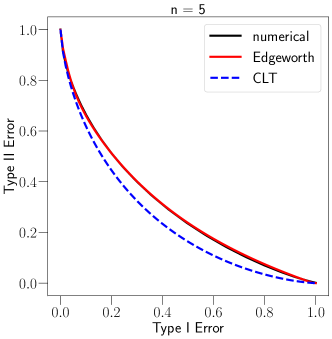
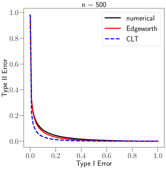
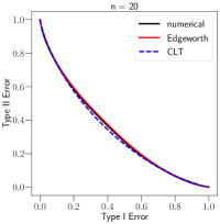
Refer to caption
Refer to caption
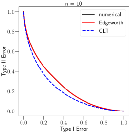
Figure 5.3: The estimation of 0.5/n14(G1+Id)n0.5superscript𝑛14superscriptsubscript𝐺1Idtensor-productabsent𝑛0.5/n^{\frac{1}{4}}(G_{1}+\text{Id})^{\otimes n}.

5.3 Privacy Guarantees for Noisy SGD
Refer to caption
Refer to caption
Refer to caption
Refer to caption
Refer to caption
Refer to caption
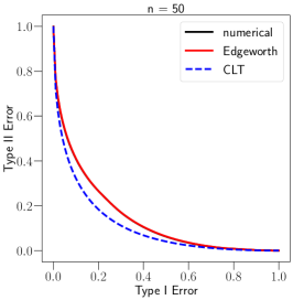
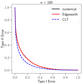
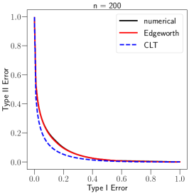
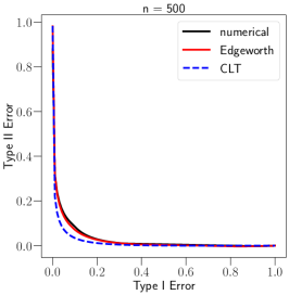
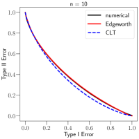
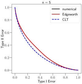
Figure 5.4: The estimation of the privacy bound for n𝑛n-step noisy SGD. The sampling rate is p=0.5/n14𝑝0.5superscript𝑛14p=0.5/n^{\frac{1}{4}} and the noise scale is σ=1𝜎1\sigma=1.

We inspect the performance of Edgeworth and CLT on estimating the privacy guarantee for n𝑛n-step noisy SGD. As introduced in Section 2, the privacy bound is of form min{g,g1}\min\left\{g,g^{-1}\right\}^{**} where g=(pG1/σ+(1p)Id)n𝑔superscript𝑝subscript𝐺1𝜎1𝑝Idtensor-productabsent𝑛g=(pG_{1/\sigma}+(1-p)\text{Id})^{\otimes n}, and the CLT estimation is Gμsubscript𝐺𝜇G_{\mu} with μ=pn(e1/σ21)𝜇𝑝𝑛superscript𝑒1superscript𝜎21\mu=p\sqrt{n(e^{1/\sigma^{2}}-1)}. For Edgeworth, note that pG1/σ+(1p)Id𝑝subscript𝐺1𝜎1𝑝IdpG_{1/\sigma}+(1-p)\text{Id} is the trade-off function of testing the standard normal distribution 𝒩(0,1)𝒩01\mathcal{N}(0,1) versus the mixture model p𝒩(1σ,1)+(1p)𝒩(0,1)𝑝𝒩1𝜎11𝑝𝒩01p\mathcal{N}(\frac{1}{\sigma},1)+(1-p)\mathcal{N}(0,1) (see Appendix C for the proof). It follows that g=T(𝒩(0,1)n,{p𝒩(1/σ,1)+(1p)𝒩(0,1)}n)𝑔𝑇𝒩superscript01tensor-productabsent𝑛superscript𝑝𝒩1𝜎11𝑝𝒩01tensor-productabsent𝑛g=T(\mathcal{N}(0,1)^{\otimes n},\left\{p\mathcal{N}(1/\sigma,1)+(1-p)\mathcal{N}(0,1)\right\}^{\otimes n}). As a result, Edgeworth can be applied by exploiting the cumulants of 𝒩(0,1)𝒩01\mathcal{N}(0,1) and p𝒩(1/σ,1)+(1p)𝒩(0,1)𝑝𝒩1𝜎11𝑝𝒩01p\mathcal{N}(1/\sigma,1)+(1-p)\mathcal{N}(0,1).

n=1𝑛1n=1 n=50𝑛50n=50 n=100𝑛100n=100 n=200𝑛200n=200 n=500𝑛500n=500
CLT 0.0004 0.0004 0.0003 0.0003 0.0003
Edgeworth 0.2504 0.2198 0.2087 0.2257 0.3048
Numerical 35.7 2138.9 4980.7 7784.8 14212.1
Table 2: Runtime for computing 0.5/n14(G1+Id)n0.5superscript𝑛14superscriptsubscript𝐺1Idtensor-productabsent𝑛0.5/n^{\frac{1}{4}}(G_{1}+\text{Id})^{\otimes n}.

Here we present the result when p=0.5/n14𝑝0.5superscript𝑛14p=0.5/n^{\frac{1}{4}}. Since the convergence of CLT requires the assumption pnν>0𝑝𝑛𝜈0p\sqrt{n}\rightarrow\nu>0 [BDLS19], this is the regime that the performance of CLT does not have theoretical guarantees, and we shall see in the following experiment that CLT significantly deviates Numerical. Nevertheless, even in this case, Edgeworth enjoys a nearly perfect match with Numerical. We also investigated the case p=0.5/n12𝑝0.5superscript𝑛12p=0.5/n^{-\frac{1}{2}}, where the convergence of CLT is guaranteed. In this regime, we shall see that Edgeworth still outperforms CLT. The results are deferred to Appendix E.2.

We let n𝑛n vary from 1 to 500. The noise scale σ𝜎\sigma is set to 1. Figure 5.3 presents the estimated g𝑔g for two representative cases n=5𝑛5n=5 and n=500𝑛500n=500. Figure 5.4 shows the final estimation after symmetrization, for a few selected values of n𝑛n. Obviously, Edgeworth is very close to Numerical for all the cases. Unlike the previous experiment, where CLT performs reasonably well when n𝑛n reaches 10, here the difference between CLT and the other two remains large even when n=500𝑛500n=500.

Table 2 presents the runtime comparison. Clearly, Numerical is not scalable. It takes more than two hours to compute 500 compositions, whereas CLT and Edgeworth can be computed within one second. The runtime of Numerical has grown three orders of magnitude from n=1𝑛1n=1 to n=500𝑛500n=500, yet the runtime of CLT and Edgeworth remains constant for all the runs.

Acknowledgments

We are grateful to Yicong Jiang for stimulating discussions in the early stages of this work. This work was supported in part by NSF through CAREER DMS-1847415, CCF-1763314, and CCF-1934876, the Wharton Dean’s Research Fund, and NIH through R01GM124111.

References

  • [Abo18] John M Abowd. The us census bureau adopts differential privacy. In Proceedings of the 24th ACM SIGKDD International Conference on Knowledge Discovery & Data Mining, pages 2867–2867, 2018.
  • [ACG+16] Martin Abadi, Andy Chu, Ian Goodfellow, H Brendan McMahan, Ilya Mironov, Kunal Talwar, and Li Zhang. Deep learning with differential privacy. In Proceedings of the 2016 ACM SIGSAC Conference on Computer and Communications Security, pages 308–318, 2016.
  • [App17] D Apple. Learning with privacy at scale. Apple Machine Learning Journal, 1(8), 2017.
  • [BBG+19] Borja Balle, Gilles Barthe, Marco Gaboardi, Justin Hsu, and Tetsuya Sato. Hypothesis testing interpretations and renyi differential privacy. arXiv preprint arXiv:1905.09982, 2019.
  • [BDLS19] Zhiqi Bu, Jinshuo Dong, Qi Long, and Weijie J Su. Deep learning with Gaussian differential privacy. arXiv preprint arXiv:1911.11607, 2019.
  • [BDRS18] Mark Bun, Cynthia Dwork, Guy N Rothblum, and Thomas Steinke. Composable and versatile privacy via truncated cdp. In Proceedings of the 50th Annual ACM SIGACT Symposium on Theory of Computing, pages 74–86, 2018.
  • [BS16] Mark Bun and Thomas Steinke. Concentrated differential privacy: Simplifications, extensions, and lower bounds. In Theory of Cryptography Conference, pages 635–658. Springer, 2016.
  • [CF38] Edmund A Cornish and Ronald A Fisher. Moments and cumulants in the specification of distributions. Revue de l’Institut international de Statistique, pages 307–320, 1938.
  • [DKM+06] Cynthia Dwork, Krishnaram Kenthapadi, Frank McSherry, Ilya Mironov, and Moni Naor. Our data, ourselves: Privacy via distributed noise generation. In Proceedings of the 24th Annual International Conference on The Theory and Applications of Cryptographic Techniques, EUROCRYPT’06, pages 486–503, Berlin, Heidelberg, 2006. Springer-Verlag.
  • [DKY17] Bolin Ding, Janardhan Kulkarni, and Sergey Yekhanin. Collecting telemetry data privately. In Advances in Neural Information Processing Systems, pages 3571–3580, 2017.
  • [DMNS06] Cynthia Dwork, Frank McSherry, Kobbi Nissim, and Adam Smith. Calibrating noise to sensitivity in private data analysis. In Proceedings of the Third Conference on Theory of Cryptography, TCC’06, pages 265–284, Berlin, Heidelberg, 2006. Springer-Verlag.
  • [DR16] Cynthia Dwork and Guy N Rothblum. Concentrated differential privacy. arXiv preprint arXiv:1603.01887, 2016.
  • [DRS19] Jinshuo Dong, Aaron Roth, and Weijie J Su. Gaussian differential privacy. arXiv preprint arXiv:1905.02383, 2019.
  • [EPK14] Úlfar Erlingsson, Vasyl Pihur, and Aleksandra Korolova. Rappor: Randomized aggregatable privacy-preserving ordinal response. In Proceedings of the 2014 ACM SIGSAC conference on computer and communications security, pages 1054–1067, 2014.
  • [FC60] Sir Ronald A Fisher and EA Cornish. The percentile points of distributions having known cumulants. Technometrics, 2(2):209–225, 1960.
  • [FJR15] Matt Fredrikson, Somesh Jha, and Thomas Ristenpart. Model inversion attacks that exploit confidence information and basic countermeasures. In Proceedings of the 22nd ACM SIGSAC Conference on Computer and Communications Security, pages 1322–1333, 2015.
  • [Hal13] Peter Hall. The bootstrap and Edgeworth expansion. Springer Science & Business Media, 2013.
  • [KOV17] Peter Kairouz, Sewoong Oh, and Pramod Viswanath. The composition theorem for differential privacy. IEEE Transactions on Information Theory, 63(6):4037–4049, 2017.
  • [KST12] Daniel Kifer, Adam Smith, and Abhradeep Thakurta. Private convex empirical risk minimization and high-dimensional regression. In Conference on Learning Theory, pages 25–1, 2012.
  • [LHC+19] Changchang Liu, Xi He, Thee Chanyaswad, Shiqiang Wang, and Prateek Mittal. Investigating statistical privacy frameworks from the perspective of hypothesis testing. Proceedings on Privacy Enhancing Technologies, 2019(3):233–254, 2019.
  • [LO11] Yehuda Lindell and Eran Omri. A practical application of differential privacy to personalized online advertising. IACR Cryptology EPrint Archive, 2011:152, 2011.
  • [Mir17] Ilya Mironov. Rényi differential privacy. In 2017 IEEE 30th Computer Security Foundations Symposium (CSF), pages 263–275. IEEE, 2017.
  • [MV16] Jack Murtagh and Salil Vadhan. The complexity of computing the optimal composition of differential privacy. In Theory of Cryptography Conference, pages 157–175. Springer, 2016.
  • [PAE+16] Nicolas Papernot, Martín Abadi, Ulfar Erlingsson, Ian Goodfellow, and Kunal Talwar. Semi-supervised knowledge transfer for deep learning from private training data. In Proceedings of the 5th International Conference on Learning Representations, 2016.
  • [SSSS17] Reza Shokri, Marco Stronati, Congzheng Song, and Vitaly Shmatikov. Membership inference attacks against machine learning models. In 2017 IEEE Symposium on Security and Privacy (SP), pages 3–18. IEEE, 2017.
  • [WZ10] Larry Wasserman and Shuheng Zhou. A statistical framework for differential privacy. Journal of the American Statistical Association, 105(489):375–389, 2010.

Appendix A The Edgeworth Approximation

We can apply Edgeworth expansion to approximate F~nsubscript~𝐹𝑛\widetilde{F}_{n} directly, following the techniques introduced in [Hal13]. Let us assume 𝒙Qsimilar-to𝒙𝑄\bm{x}\sim Q. Denote

XQ=Tn𝔼Q[Tn]𝕍arQ(Tn)=i=1n(Liμi)i=1nσi2,subscript𝑋𝑄subscript𝑇𝑛subscript𝔼𝑄delimited-[]subscript𝑇𝑛𝕍subscriptar𝑄subscript𝑇𝑛superscriptsubscript𝑖1𝑛subscript𝐿𝑖subscript𝜇𝑖superscriptsubscript𝑖1𝑛subscriptsuperscript𝜎2𝑖X_{Q}=\frac{T_{n}-\mathbb{E}_{Q}[T_{n}]}{\sqrt{\mathbb{V}\text{ar}_{Q}(T_{n})}}=\frac{\sum_{i=1}^{n}(L_{i}-\mu_{i})}{\sqrt{\sum_{i=1}^{n}\sigma^{2}_{i}}}, (A.1)

where μisubscript𝜇𝑖\mu_{i} and σi2superscriptsubscript𝜎𝑖2\sigma_{i}^{2} are the mean and variance of Lisubscript𝐿𝑖L_{i} under the distribution Qisubscript𝑄𝑖Q_{i}. The characteristic function of XQsubscript𝑋𝑄X_{Q} is

χn(t)=exp(i=1κ~r(XQ)(it)rr!),subscript𝜒𝑛𝑡superscriptsubscript𝑖1subscript~𝜅𝑟subscript𝑋𝑄superscript𝑖𝑡𝑟𝑟\chi_{n}(t)=\exp\left(\sum_{i=1}^{\infty}\tilde{\kappa}_{r}(X_{Q})\frac{(it)^{r}}{r!}\right),

where κ~r(XQ)subscript~𝜅𝑟subscript𝑋𝑄\tilde{\kappa}_{r}(X_{Q}) is the r𝑟r-th cumulant of XQsubscript𝑋𝑄X_{Q}. Details of how to compute the cumulants are summarized in Appendix B. Let σn=i=1nσi2subscript𝜎𝑛superscriptsubscript𝑖1𝑛subscriptsuperscript𝜎2𝑖\sigma_{n}=\sqrt{\sum_{i=1}^{n}\sigma^{2}_{i}}. Particularly we have

κ~1(XQ)subscript~𝜅1subscript𝑋𝑄\displaystyle\tilde{\kappa}_{1}(X_{Q}) =𝔼Q(XQ)=0,absentsubscript𝔼𝑄subscript𝑋𝑄0\displaystyle=\mathbb{E}_{Q}(X_{Q})=0, (A.2)
κ~2(XQ)subscript~𝜅2subscript𝑋𝑄\displaystyle\tilde{\kappa}_{2}(X_{Q}) =𝕍arQ(XQ)=1,absent𝕍subscriptar𝑄subscript𝑋𝑄1\displaystyle=\mathbb{V}\text{ar}_{Q}(X_{Q})=1,
\displaystyle\vdots
κ~r(XQ)subscript~𝜅𝑟subscript𝑋𝑄\displaystyle\tilde{\kappa}_{r}(X_{Q}) =κ~r(σn1i=1n(Liμi))absentsubscript~𝜅𝑟superscriptsubscript𝜎𝑛1superscriptsubscript𝑖1𝑛subscript𝐿𝑖subscript𝜇𝑖\displaystyle=\tilde{\kappa}_{r}\left(\sigma_{n}^{-1}\sum_{i=1}^{n}(L_{i}-\mu_{i})\right)
=σnri=1nκ~r(Li),r>2.formulae-sequenceabsentsuperscriptsubscript𝜎𝑛𝑟superscriptsubscript𝑖1𝑛subscript~𝜅𝑟subscript𝐿𝑖for-all𝑟2\displaystyle=\sigma_{n}^{-r}\sum_{i=1}^{n}\tilde{\kappa}_{r}(L_{i}),\;\;\forall r>2.

We will denote the sum of n𝑛n cumulants by 𝜿~r=i=1nκ~r(Li)subscriptbold-~𝜿𝑟superscriptsubscript𝑖1𝑛subscript~𝜅𝑟subscript𝐿𝑖\bm{\tilde{\kappa}}_{r}=\sum_{i=1}^{n}\tilde{\kappa}_{r}(L_{i}). Under the series expansion of the exponential function, we will have

χn(t)=subscript𝜒𝑛𝑡absent\displaystyle\chi_{n}(t)= exp(t22)exp(r=3σnrr!𝜿~r(it)r)superscript𝑡22superscriptsubscript𝑟3superscriptsubscript𝜎𝑛𝑟𝑟subscriptbold-~𝜿𝑟superscript𝑖𝑡𝑟\displaystyle\exp\left(-\frac{t^{2}}{2}\right)\exp\left(\sum_{r=3}^{\infty}\frac{\sigma_{n}^{-r}}{r!}\bm{\tilde{\kappa}}_{r}(it)^{r}\right) (A.3)
\displaystyle\approx exp(t22)exp(r=3,4σnrr!𝜿~r(it)r)superscript𝑡22subscript𝑟34superscriptsubscript𝜎𝑛𝑟𝑟subscriptbold-~𝜿𝑟superscript𝑖𝑡𝑟\displaystyle\exp\left(-\frac{t^{2}}{2}\right)\exp\left(\sum_{r=3,4}\frac{\sigma_{n}^{-r}}{r!}\bm{\tilde{\kappa}}_{r}(it)^{r}\right)
\displaystyle\approx exp(t22)(1+σn316𝜿~3(it)3r1(it)\displaystyle\exp\left(-\frac{t^{2}}{2}\right)\bigg{(}1+\sigma_{n}^{-3}\cdot\overbrace{\frac{1}{6}\bm{\tilde{\kappa}}_{3}(it)^{3}}^{r_{1}(it)}
+σn4124𝜿~4(it)4r2(it)+σn6172𝜿~32(it)6r3(it)).\displaystyle+\sigma_{n}^{-4}\cdot\overbrace{\frac{1}{24}\bm{\tilde{\kappa}}_{4}(it)^{4}}^{r_{2}(it)}+\sigma_{n}^{-6}\cdot\overbrace{\frac{1}{72}\bm{\tilde{\kappa}}_{3}^{2}(it)^{6}}^{r_{3}(it)}\bigg{)}.

Since χn(t)=eith𝑑F~n(h)subscript𝜒𝑛𝑡superscript𝑒𝑖𝑡differential-dsubscript~𝐹𝑛\chi_{n}(t)=\int e^{ith}d\widetilde{F}_{n}(h) and et2/2=eith𝑑Φ(h)superscript𝑒superscript𝑡22superscript𝑒𝑖𝑡differential-dΦe^{-t^{2}/2}=\int e^{ith}d\Phi(h), we can obtain the corresponding “inverse” expansion:

F~n(h)Φ(h)+σn3R1(h)+σn4R2(h)+σn6R3(h),subscript~𝐹𝑛Φsuperscriptsubscript𝜎𝑛3subscript𝑅1superscriptsubscript𝜎𝑛4subscript𝑅2superscriptsubscript𝜎𝑛6subscript𝑅3\widetilde{F}_{n}(h)\approx\Phi(h)+\sigma_{n}^{-3}\cdot R_{1}(h)+\sigma_{n}^{-4}\cdot R_{2}(h)+\sigma_{n}^{-6}\cdot R_{3}(h), (A.4)

and Rj(h)subscript𝑅𝑗R_{j}(h) is a function whose Fourier-Stieljes transform equals rj(it)et2/2subscript𝑟𝑗𝑖𝑡superscript𝑒superscript𝑡22r_{j}(it)e^{-t^{2}/2}:

eith𝑑Rj(h)=rj(it)et2/2.superscriptsubscriptsuperscript𝑒𝑖𝑡differential-dsubscript𝑅𝑗subscript𝑟𝑗𝑖𝑡superscript𝑒superscript𝑡22\int_{-\infty}^{\infty}e^{ith}dR_{j}(h)=r_{j}(it)e^{-t^{2}/2}.

Let D𝐷D denote the differential operator d/dh𝑑𝑑d/dh. We have

et2/2=(it)jeithd{DjΦ(h)}superscript𝑒superscript𝑡22superscript𝑖𝑡𝑗superscriptsubscriptsuperscript𝑒𝑖𝑡𝑑superscript𝐷𝑗Φe^{-t^{2}/2}=(-it)^{-j}\int_{-\infty}^{\infty}e^{ith}d\left\{D^{j}\Phi(h)\right\}

and hence

eithd{(D)jΦ(h)}=(it)jet2/2.superscriptsubscriptsuperscript𝑒𝑖𝑡𝑑superscript𝐷𝑗Φsuperscript𝑖𝑡𝑗superscript𝑒superscript𝑡22\int_{-\infty}^{\infty}e^{ith}d\left\{(-D)^{j}\Phi(h)\right\}=(it)^{j}e^{-t^{2}/2}.

Let us interpret rj(D)subscript𝑟𝑗𝐷r_{j}(-D) as a polynomial in D𝐷D, we then obtain

eithd{rj(D)Φ(h)}=rj(it)et2/2.superscriptsubscriptsuperscript𝑒𝑖𝑡𝑑subscript𝑟𝑗𝐷Φsubscript𝑟𝑗𝑖𝑡superscript𝑒superscript𝑡22\int_{-\infty}^{\infty}e^{ith}d\left\{r_{j}(-D)\Phi(h)\right\}=r_{j}(it)e^{-t^{2}/2}.

Consequently,

Rj(h)=rj(D)ϕ(h).subscript𝑅𝑗subscript𝑟𝑗𝐷italic-ϕR_{j}(h)=r_{j}(-D)\phi(h). (A.5)

It is well known that for j1𝑗1j\geq 1,

(D)jΦ(h)=Hej1(h)ϕ(h)superscript𝐷𝑗Φ𝐻subscript𝑒𝑗1italic-ϕ(-D)^{j}\Phi(h)=-He_{j-1}(h)\phi(h) (A.6)

and Hej𝐻subscript𝑒𝑗He_{j}s are the Hermite polynomials:

He0(h)𝐻subscript𝑒0\displaystyle He_{0}(h) =1,absent1\displaystyle=1,\;\; (A.7)
He1(h)𝐻subscript𝑒1\displaystyle He_{1}(h) =h,absent\displaystyle=h,\;\;
He2(h)𝐻subscript𝑒2\displaystyle He_{2}(h) =h21,absentsuperscript21\displaystyle=h^{2}-1,
He3(h)𝐻subscript𝑒3\displaystyle He_{3}(h) =h33h,absentsuperscript33\displaystyle=h^{3}-3h,\;\;
He4(h)𝐻subscript𝑒4\displaystyle He_{4}(h) =h46h2+3,absentsuperscript46superscript23\displaystyle=h^{4}-6h^{2}+3,
He5(h)𝐻subscript𝑒5\displaystyle He_{5}(h) =h510h3+15h,absentsuperscript510superscript315\displaystyle=h^{5}-10h^{3}+15h,\;\;
He6(h)𝐻subscript𝑒6\displaystyle He_{6}(h) =h615h4+45h215,absentsuperscript615superscript445superscript215\displaystyle=h^{6}-15h^{4}+45h^{2}-15,
He7(h)𝐻subscript𝑒7\displaystyle He_{7}(h) =h721h5+105h3,absentsuperscript721superscript5105superscript3\displaystyle=h^{7}-21h^{5}+105h^{3},
\displaystyle\ldots

Combine equations A.4, A.5, A.6 and A.7 we can deduce the final result:

F~n(h)subscript~𝐹𝑛\displaystyle\widetilde{F}_{n}(h) \displaystyle\approx Φ(h)+σn316𝜿~3(h21)ϕ(h)\displaystyle\Phi(h)+\sigma_{n}^{-3}\cdot-\frac{1}{6}\bm{\tilde{\kappa}}_{3}(h^{2}-1)\phi(h) (A.8)
+σn4124𝜿~4(h33h)ϕ(h)\displaystyle+\sigma_{n}^{-4}\cdot-\frac{1}{24}\bm{\tilde{\kappa}}_{4}(h^{3}-3h)\phi(h)
+σn6172𝜿~32(h510h3+15h)ϕ(h).\displaystyle+\sigma_{n}^{-6}\cdot-\frac{1}{72}\bm{\tilde{\kappa}}_{3}^{2}(h^{5}-10h^{3}+15h)\phi(h).

In A.3, the truncation happens in both the second and third line. In the second line, we truncated terms where r5𝑟5r\geq 5. In the following line, we apply the series expansion to the exponential function, and we stopped after taking t1:=σn316𝜿~3(it)3assignsubscript𝑡1subscriptsuperscript𝜎3𝑛16subscriptbold-~𝜿3superscript𝑖𝑡3t_{1}:=\sigma^{-3}_{n}\cdot\frac{1}{6}\bm{\tilde{\kappa}}_{3}(it)^{3}, t2:=σn4124𝜿~4(it)4assignsubscript𝑡2subscriptsuperscript𝜎4𝑛124subscriptbold-~𝜿4superscript𝑖𝑡4t_{2}:=\sigma^{-4}_{n}\cdot\frac{1}{24}\bm{\tilde{\kappa}}_{4}(it)^{4} and the square of t1subscript𝑡1t_{1}.

The error stems from truncating r5𝑟5r\geq 5 terms in the second line will be dominated by 1120σn5𝜿~5(it)51120superscriptsubscript𝜎𝑛5subscriptbold-~𝜿5superscript𝑖𝑡5\dfrac{1}{120}\sigma_{n}^{-5}\bm{\tilde{\kappa}}_{5}(it)^{5} in the series expansion. The error stems from truncating the expansion of r=3,4𝑟34r=3,4 terms in the following line will be dominated by the square of t2subscript𝑡2t_{2}: σn81576𝜿~42(it)8subscriptsuperscript𝜎8𝑛1576subscriptsuperscriptbold-~𝜿24superscript𝑖𝑡8\sigma^{-8}_{n}\cdot\frac{1}{576}\bm{\tilde{\kappa}}^{2}_{4}(it)^{8}.

Since all Lisubscript𝐿𝑖L_{i}’s are identically distributed, the cumulants of L1,Lnsubscript𝐿1subscript𝐿𝑛L_{1},\ldots L_{n} take the same value for any fixed order. Therefore, σ1==σn=σsubscript𝜎1subscript𝜎𝑛𝜎\sigma_{1}=\cdots=\sigma_{n}=\sigma and κ~r=κ~r(L1)==κ~r(Ln)subscript~𝜅𝑟subscript~𝜅𝑟subscript𝐿1subscript~𝜅𝑟subscript𝐿𝑛\tilde{\kappa}_{r}=\tilde{\kappa}_{r}(L_{1})=\cdots=\tilde{\kappa}_{r}(L_{n}). As a consequence, we have σn=nσsubscript𝜎𝑛𝑛𝜎\sigma_{n}=\sqrt{n}\sigma and 𝜿~r=nκ~rsubscriptbold-~𝜿𝑟𝑛subscript~𝜅𝑟\bm{\tilde{\kappa}}_{r}=n\tilde{\kappa}_{r}. This leads to

σn3𝜿~3(it)3n1/2(it)3,similar-tosubscriptsuperscript𝜎3𝑛subscriptbold-~𝜿3superscript𝑖𝑡3superscript𝑛12superscript𝑖𝑡3\displaystyle\sigma^{-3}_{n}\cdot\bm{\tilde{\kappa}}_{3}(it)^{3}\sim n^{-1/2}(it)^{3}, (A.9)
σn4𝜿~4(it)4n1(it)4,similar-tosubscriptsuperscript𝜎4𝑛subscriptbold-~𝜿4superscript𝑖𝑡4superscript𝑛1superscript𝑖𝑡4\displaystyle\sigma^{-4}_{n}\cdot\bm{\tilde{\kappa}}_{4}(it)^{4}\sim n^{-1}(it)^{4},
σn6𝜿~32(it)6n1(it)6,similar-tosubscriptsuperscript𝜎6𝑛subscriptsuperscriptbold-~𝜿23superscript𝑖𝑡6superscript𝑛1superscript𝑖𝑡6\displaystyle\sigma^{-6}_{n}\cdot\bm{\tilde{\kappa}}^{2}_{3}(it)^{6}\sim n^{-1}(it)^{6},
σn8𝜿~42(it)8n2(it)8,similar-tosubscriptsuperscript𝜎8𝑛subscriptsuperscriptbold-~𝜿24superscript𝑖𝑡8superscript𝑛2superscript𝑖𝑡8\displaystyle\sigma^{-8}_{n}\cdot\bm{\tilde{\kappa}}^{2}_{4}(it)^{8}\sim n^{-2}(it)^{8},
σn5𝜿~5(it)5n3/2(it)5.similar-tosubscriptsuperscript𝜎5𝑛subscriptbold-~𝜿5superscript𝑖𝑡5superscript𝑛32superscript𝑖𝑡5\displaystyle\sigma^{-5}_{n}\cdot\bm{\tilde{\kappa}}_{5}(it)^{5}\sim n^{-3/2}(it)^{5}.

Hence the error for approximating χn(t)subscript𝜒𝑛𝑡\chi_{n}(t) is upper bounded by O(n2(it)8+n3/2(it)5)𝑂superscript𝑛2superscript𝑖𝑡8superscript𝑛32superscript𝑖𝑡5O\left(n^{-2}(it)^{8}+n^{-3/2}(it)^{5}\right). Next, we connect the characteristic function to CDF F~n(h)subscript~𝐹𝑛\widetilde{F}_{n}(h). From equations A.5 and A.6, we know the error term will be transformed into O(n2He7(h)+n3/2He4(h))𝑂superscript𝑛2𝐻subscript𝑒7superscript𝑛32𝐻subscript𝑒4O\left(n^{-2}He_{7}(h)+n^{-3/2}He_{4}(h)\right) as approximating F~n(h)subscript~𝐹𝑛\widetilde{F}_{n}(h), which is O(n2h7+n3/2h3)𝑂superscript𝑛2superscript7superscript𝑛32superscript3O\left(n^{-2}h^{7}+n^{-3/2}h^{3}\right).

Appendix B Computing Cumulants From Moments

The cumulants of a random variable X𝑋X are defined using the cumulant-generating function K(t)𝐾𝑡K(t). It is the natural logarithm of the moment-generating function:

K(t)=log𝔼(etX),𝐾𝑡𝔼superscript𝑒𝑡𝑋K(t)=\log\operatorname{\mathbb{E}}\left(e^{tX}\right),

and the cumulants are the coefficients in the Taylor expansion of K(t)𝐾𝑡K(t) about the origin:

K(t)=log𝔼(etX)=r=0κrtr/r!.𝐾𝑡𝔼superscript𝑒𝑡𝑋superscriptsubscript𝑟0subscript𝜅𝑟superscript𝑡𝑟𝑟K(t)=\log\operatorname{\mathbb{E}}\left(e^{tX}\right)=\sum_{r=0}^{\infty}\kappa_{r}t^{r}/r!.

For any integer r0𝑟0r\geq 0, the r𝑟r-th order non-central moment of X𝑋X is μr=𝔼(Xr)subscript𝜇𝑟𝔼superscript𝑋𝑟\mu_{r}=\operatorname{\mathbb{E}}(X^{r}). Recall the Taylor expansion of the moment-generating function M(t)𝑀𝑡M(t) about the origin

M(t)=𝔼(etX)=r=0μrtr/r!=exp(K(t)).𝑀𝑡𝔼superscript𝑒𝑡𝑋superscriptsubscript𝑟0subscript𝜇𝑟superscript𝑡𝑟𝑟𝐾𝑡M(t)=\operatorname{\mathbb{E}}\left(e^{tX}\right)=\sum_{r=0}^{\infty}\mu_{r}t^{r}/r!=\exp\left(K(t)\right).

The cumulants can be recovered in terms of the moments and vice versa. In general,

κr=k=1r(1)k1(k1)!Br,k(μ1,,μrk+1)subscript𝜅𝑟superscriptsubscript𝑘1𝑟superscript1𝑘1𝑘1subscript𝐵𝑟𝑘subscript𝜇1subscript𝜇𝑟𝑘1\kappa_{r}=\sum_{k=1}^{r}(-1)^{k-1}(k-1)!B_{r,k}(\mu_{1},\ldots,\mu_{r-k+1})

where Bn,ksubscript𝐵𝑛𝑘B_{n,k} are Bell polynomials. The relationship between the first few cumulants and moments is as the following:

κ0=0,subscript𝜅00\displaystyle\kappa_{0}=0,
κ1=μ1,subscript𝜅1subscript𝜇1\displaystyle\kappa_{1}=\mu_{1},
κ2=μ2μ12,subscript𝜅2subscript𝜇2superscriptsubscript𝜇12\displaystyle\kappa_{2}=\mu_{2}-\mu_{1}^{2},
κ3=μ33μ2μ1+2μ13,subscript𝜅3subscript𝜇33subscript𝜇2subscript𝜇12subscriptsuperscript𝜇31\displaystyle\kappa_{3}=\mu_{3}-3\mu_{2}\mu_{1}+2\mu^{3}_{1},
κ4=μ44μ3μ13μ22+12μ2μ126μ14.subscript𝜅4subscript𝜇44subscript𝜇3subscript𝜇13subscriptsuperscript𝜇2212subscript𝜇2superscriptsubscript𝜇126subscriptsuperscript𝜇41\displaystyle\kappa_{4}=\mu_{4}-4\mu_{3}\mu_{1}-3\mu^{2}_{2}+12\mu_{2}\mu_{1}^{2}-6\mu^{4}_{1}.

Appendix C 𝒩(0,1)𝒩01\mathcal{N}(0,1) vs p𝒩(μ,1)+(1p)𝒩(0,1))p\mathcal{N}(\mu,1)+(1-p)\mathcal{N}(0,1))

Let P𝑃P be the standard normal distribution 𝒩(0,1)𝒩01\mathcal{N}(0,1) and Q𝑄Q be a mixture model p𝒩(μ,1)+(1p)𝒩(0,1)𝑝𝒩𝜇11𝑝𝒩01p\mathcal{N}(\mu,1)+(1-p)\mathcal{N}(0,1) with μ0𝜇0\mu\geqslant 0. We now show that

Lemma C.1.
T(P,Q)=pGμ+(1p)Id.𝑇𝑃𝑄𝑝subscript𝐺𝜇1𝑝IdT(P,Q)=pG_{\mu}+(1-p)\mathrm{Id}.
Proof.

The likelihood ratio between Q𝑄Q and P𝑃P is

pe12(xμ)2+12x2+1p=peμx12μ2+1p.𝑝superscripte12superscript𝑥𝜇212superscript𝑥21𝑝𝑝superscripte𝜇𝑥12superscript𝜇21𝑝p\mathrm{e}^{-\frac{1}{2}(x-\mu)^{2}+\frac{1}{2}x^{2}}+1-p=p\mathrm{e}^{\mu x-\frac{1}{2}\mu^{2}}+1-p.

Since μ0𝜇0\mu\geqslant 0, likelihood ratio tests are thresholding, i.e., {x:x>h}conditional-set𝑥𝑥\{x:x>h\}. The type I and type II errors are

α𝛼\displaystyle\alpha =P{x:x>h}=1Φ(h),absent𝑃conditional-set𝑥𝑥1Φ\displaystyle=P\{x:x>h\}=1-\Phi(h),
β𝛽\displaystyle\beta =Q{x:xh}absent𝑄conditional-set𝑥𝑥\displaystyle=Q\{x:x\leqslant h\}
=p𝔼x𝒩(μ,1)[1{x:xh}]+(1p)𝔼x𝒩(0,1)[1{x:xh}]absent𝑝subscript𝔼similar-to𝑥𝒩𝜇1subscript1conditional-set𝑥𝑥1𝑝subscript𝔼similar-to𝑥𝒩01subscript1conditional-set𝑥𝑥\displaystyle=p\operatorname{\mathbb{E}}_{x\sim\mathcal{N}(\mu,1)}[1_{\{x:x\leqslant h\}}]+(1-p)\operatorname{\mathbb{E}}_{x\sim\mathcal{N}(0,1)}[1_{\{x:x\leqslant h\}}]
=pΦ(hμ)+(1p)Φ(h).absent𝑝Φ𝜇1𝑝Φ\displaystyle=p\Phi(h-\mu)+(1-p)\Phi(h).

Inverting the first formula, we have h=Φ1(1α)superscriptΦ11𝛼h=\Phi^{-1}(1-\alpha). So

β=pΦ(hμ)+(1p)Φ(h)=pΦ(Φ1(1α)μ)+(1p)(1α)𝛽𝑝Φ𝜇1𝑝Φ𝑝ΦsuperscriptΦ11𝛼𝜇1𝑝1𝛼\beta=p\Phi(h-\mu)+(1-p)\Phi(h)=p\Phi(\Phi^{-1}(1-\alpha)-\mu)+(1-p)(1-\alpha)

Making use of the known expression Gμ(α)=Φ(Φ1(1α)μ)subscript𝐺𝜇𝛼ΦsuperscriptΦ11𝛼𝜇G_{\mu}(\alpha)=\Phi\big{(}\Phi^{-1}(1-\alpha)-\mu\big{)} and Id(α)=1αId𝛼1𝛼\mathrm{Id}(\alpha)=1-\alpha, we have

T(P,Q)(α)=β=pGμ(α)+(1p)Id(α).𝑇𝑃𝑄𝛼𝛽𝑝subscript𝐺𝜇𝛼1𝑝Id𝛼T(P,Q)(\alpha)=\beta=pG_{\mu}(\alpha)+(1-p)\mathrm{Id}(\alpha).

Appendix D Details of the Numerical Method

D.1 Proof of Lemma 5.1

Proof.

By definition of convex conjugacy, δδ1(ε)𝛿subscript𝛿1𝜀\delta\geqslant\delta_{1}(\varepsilon) if and only if f(x)1δeεx𝑓𝑥1𝛿superscripte𝜀𝑥f(x)\geqslant 1-\delta-\mathrm{e}^{\varepsilon}x for all x[0,1]𝑥01x\in[0,1]. Since f=T(P,Q)𝑓𝑇𝑃𝑄f=T(P,Q) characterizes optimal testing rules, f(x)1δeεx𝑓𝑥1𝛿superscripte𝜀𝑥f(x)\geqslant 1-\delta-\mathrm{e}^{\varepsilon}x for any x[0,1]𝑥01x\in[0,1] if and only if for any event E𝐸E, Q[E]eεP[E]+δ𝑄delimited-[]𝐸superscripte𝜀𝑃delimited-[]𝐸𝛿Q[E]\leqslant\mathrm{e}^{\varepsilon}P[E]+\delta. That is,

δ1(ε)subscript𝛿1𝜀\displaystyle\delta_{1}(\varepsilon) =min{δ:Q[E]eεP[E]+δ,E}absent:𝛿𝑄delimited-[]𝐸superscripte𝜀𝑃delimited-[]𝐸𝛿for-all𝐸\displaystyle=\min\{\delta:Q[E]\leqslant\mathrm{e}^{\varepsilon}P[E]+\delta,\forall E\}
=maxEQ[E]eεP[E]absentsubscript𝐸𝑄delimited-[]𝐸superscripte𝜀𝑃delimited-[]𝐸\displaystyle=\max_{E}Q[E]-\mathrm{e}^{\varepsilon}P[E]
=maxEE[q(x)eεp(x)]dμ(x).absentsubscript𝐸subscript𝐸delimited-[]𝑞𝑥superscripte𝜀𝑝𝑥differential-d𝜇𝑥\displaystyle=\max_{E}\int_{E}\big{[}q(x)-\mathrm{e}^{\varepsilon}p(x)\big{]}\mathrm{d}\mu(x).

Obviously, the maximum is attained at the event that the integrand being non-negative. That is, E={x:q(x)eεp(x)0}𝐸conditional-set𝑥𝑞𝑥superscripte𝜀𝑝𝑥0E=\{x:q(x)-\mathrm{e}^{\varepsilon}p(x)\geqslant 0\}. Therefore,

δ1(ε)=(qeεp)+dμ.subscript𝛿1𝜀subscript𝑞superscripte𝜀𝑝differential-d𝜇\delta_{1}(\varepsilon)=\int\big{(}q-\mathrm{e}^{\varepsilon}p\big{)}_{+}\mathrm{d}\mu.

D.2 Proof of Lemma 5.2

Proof.

By definition of tensor-product\otimes and Lemma 5.1, we have

δ(ε)subscript𝛿tensor-product𝜀\displaystyle\delta_{\otimes}(\varepsilon) =1+(f1f2)(eε)absent1superscripttensor-productsubscript𝑓1subscript𝑓2superscripte𝜀\displaystyle=1+(f_{1}\otimes f_{2})^{*}(-\mathrm{e}^{\varepsilon})
=1+(T(P1×P2,Q1×Q2))(eε)absent1superscript𝑇subscript𝑃1subscript𝑃2subscript𝑄1subscript𝑄2superscripte𝜀\displaystyle=1+\big{(}T(P_{1}\times P_{2},Q_{1}\times Q_{2})\big{)}^{*}(-\mathrm{e}^{\varepsilon}) (Def of )\displaystyle(\text{Def of }\otimes)
=(q1(x)q2(y)eεp1(x)p2(y))+dxdyabsentdouble-integralsubscriptsubscript𝑞1𝑥subscript𝑞2𝑦superscripte𝜀subscript𝑝1𝑥subscript𝑝2𝑦differential-d𝑥differential-d𝑦\displaystyle=\iint\big{(}q_{1}(x)q_{2}(y)-\mathrm{e}^{\varepsilon}p_{1}(x)p_{2}(y)\big{)}_{+}\mathrm{d}x\mathrm{d}y (Lemma 5.1)Lemma 5.1\displaystyle(\text{Lemma }\ref{lem:delta_1})
=q2(y)(q1(x)eεp1(x)p2(y)q2(y))+dxdyabsentdouble-integralsubscript𝑞2𝑦subscriptsubscript𝑞1𝑥superscripte𝜀subscript𝑝1𝑥subscript𝑝2𝑦subscript𝑞2𝑦differential-d𝑥differential-d𝑦\displaystyle=\iint q_{2}(y)\cdot\Big{(}q_{1}(x)-\mathrm{e}^{\varepsilon}p_{1}(x)\cdot\tfrac{p_{2}(y)}{q_{2}(y)}\Big{)}_{+}\mathrm{d}x\mathrm{d}y (q2(y)0)subscript𝑞2𝑦0\displaystyle(q_{2}(y)\geqslant 0)
=q2(y)(q1(x)eεL2(y)p1(x))+dxdyabsentdouble-integralsubscript𝑞2𝑦subscriptsubscript𝑞1𝑥superscripte𝜀subscript𝐿2𝑦subscript𝑝1𝑥differential-d𝑥differential-d𝑦\displaystyle=\iint q_{2}(y)\cdot\Big{(}q_{1}(x)-\mathrm{e}^{\varepsilon-L_{2}(y)}p_{1}(x)\Big{)}_{+}\mathrm{d}x\mathrm{d}y (Def of L2)Def of subscript𝐿2\displaystyle(\text{Def of }L_{2})
=q2(y)[(q1(x)eεL2(y)p1(x))+dx]dyabsentsubscript𝑞2𝑦delimited-[]subscriptsubscript𝑞1𝑥superscripte𝜀subscript𝐿2𝑦subscript𝑝1𝑥differential-d𝑥differential-d𝑦\displaystyle=\int q_{2}(y)\cdot\Big{[}\int\big{(}q_{1}(x)-\mathrm{e}^{\varepsilon-L_{2}(y)}p_{1}(x)\big{)}_{+}\mathrm{d}x\Big{]}\mathrm{d}y (Fubini)Fubini\displaystyle(\text{Fubini})
=q2(y)δ1(εL2(y))dy.absentsubscript𝑞2𝑦subscript𝛿1𝜀subscript𝐿2𝑦differential-d𝑦\displaystyle=\int q_{2}(y)\cdot\delta_{1}\big{(}\varepsilon-L_{2}(y)\big{)}\mathrm{d}y. (Lemma 5.1 on δ1)Lemma 5.1 on subscript𝛿1\displaystyle(\text{Lemma }\ref{lem:delta_1}\text{ on }\delta_{1})

Appendix E Privacy Guarantees for Noisy SGD with Sampling Rate p=0.5n𝑝0.5𝑛p=\frac{0.5}{\sqrt{n}}
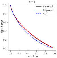
Refer to caption
Refer to caption
Refer to caption
Refer to caption
Figure E.1: The estimation of 0.5/n12(G1+Id)n0.5superscript𝑛12superscriptsubscript𝐺1Idtensor-productabsent𝑛0.5/n^{\frac{1}{2}}(G_{1}+\text{Id})^{\otimes n}.
Refer to caption
Refer to caption
Refer to caption
Refer to caption
Figure E.2: The estimation of the privacy bound for n𝑛n-step noisy SGD. The sampling rate is p=0.5/n12𝑝0.5superscript𝑛12p=0.5/n^{\frac{1}{2}} and the noise scale is σ=1𝜎1\sigma=1.

In Section 5.3 we present the result when the sampling rate p=0.5/n14𝑝0.5superscript𝑛14p=0.5/n^{\frac{1}{4}}. Since the convergence of CLT requires the assumption pnν>0𝑝𝑛𝜈0p\sqrt{n}\rightarrow\nu>0 [BDLS19], that is a regime where the performance of CLT does not have theoretical guarantees. Here we present the results when p=0.5/n12𝑝0.5superscript𝑛12p=0.5/n^{\frac{1}{2}}, where the convergence of CLT is guaranteed. However, we still observe that Edgeworth outperforms CLT. See Figure E.2 and E.2 for the comparison.