Least Squares Estimation of a Quasiconvex Regression Function

Abstract

We develop a new approach for the estimation of a multivariate function based on the economic axioms of quasiconvexity (and monotonicity). On the computational side, we prove the existence of the quasiconvex constrained least squares estimator (LSE) and provide a characterization of the function space to compute the LSE via a mixed integer quadratic programme. On the theoretical side, we provide finite sample risk bounds for the LSE via a sharp oracle inequality. Our results allow for errors to depend on the covariates and to have only two finite moments. We illustrate the superior performance of the LSE against some competing estimators via simulation. Finally, we use the LSE to estimate the production function for the Japanese plywood industry and the cost function for hospitals across the US.

1 Introduction

Production analysis has been an indispensable tool for economists, managers, and engineers in evaluating a firm’s performance. Reliable estimates of production functions are of great importance because they can assist in accurate decision making. In this context, regression models enable us to identify relationships among resources and products.

Consider a production process that uses $d$ different resources to produce a single product or output, $Y\in\mathbb{R}$. The resources consumed are called the inputs, and we denote their quantity by $\boldsymbol{X}\in\mathbb{R}^{d}$. We consider the following regression model

$$Y=\varphi(\boldsymbol{X})+\varepsilon,$$ (1)

where the random variable $\varepsilon$ satisfies $\mathbb{E}(\varepsilon|\boldsymbol{X})=0$ and $\mathbb{E}(\varepsilon^{2}|\boldsymbol{X})<\infty$ for almost every $\boldsymbol{X}$. Given $n$ i.i.d. observations $\{(\boldsymbol{X}_{j},Y_{j})\}_{j=1}^{n}$ from the regression model (1), the goal of the paper is to estimate the unknown production function $\varphi:\mathbb{R}^{d}\to\mathbb{R}$, subject to some basic shape constraints imposed by economic axioms.

Production functions are linked to cost functions through a dual relationship,so axioms that hold for production functions imply similar axioms for cost functions (Shephard,, 1953; Diewert,, 1982). We will thus frame our discussion of axiomatic properties primarily in terms of production functions, recognizing that through duality, similar axioms are required for cost functions. Microeconomic theory often implies qualitative assumptions on production functions, and the most prominent of those assumptions is the monotonicity axiom (Varian,, 1992, page 6), which says that an increase in input resources should lead to no less output. This argument is common and reasonable for establishments facing competition, see e.g., Beattie et al., (1985, Pages 10–11) and Chambers, (1988). Formally, the monotonicity axiom implies that

$$\text{if }\boldsymbol{X}_{1}\leq\boldsymbol{X}_{2},\text{ then }{\varphi(\boldsymbol{X}_{1})\leq\varphi(\boldsymbol{X}_{2})},$$ (2)

where for two vectors $\boldsymbol{a}:=(a_{1},\ldots,a_{d}),\boldsymbol{b}:=(b_{1},\ldots,b_{d})\in\mathbb{R}^{d}$, we say $\boldsymbol{a}\leq\boldsymbol{b}$ if $a_{i}\leq b_{i}$ for all $i\in\{1,\ldots,d\}$.

For a given output level $y,$ define the input requirement set $V(y)\subset\mathbb{R}^{d}$ as the set of all input vectors $\boldsymbol{x}$ that produce at least $y$ units of output, i.e. $V(y):=\{\boldsymbol{x}:\varphi(\boldsymbol{x})\geq y\}.$ Another prominent assumption about the production function is that the input requirement set $V(y)$ is convex for every $y\in\mathbb{R}$, i.e.

$$\text{if }\boldsymbol{x}_{1},\boldsymbol{x}_{2}\in V(y),\text{ then }\lambda\boldsymbol{x}_{1}+(1-\lambda)\boldsymbol{x}_{2}\in V(y)\text{ for all }\lambda\in[0,1].$$ (3)

The economic motivation for this assumption is based on the fact that for most production technologies there are optimal proportions in which inputs should be used and that deviations from the optimal proportion by decreasing the level of one input, such as capital, will require more than a proportional increase in another input, such as labor (Johnson and Jiang,, 2018). Furthermore Varian, (1992, Page 82) argues that even if the production technology does not justify convexity, if the prices for inputs are positive, then operating in a nonconvex region of the input requirement set would be economically inefficient and should be avoided.

Estimates of production and cost functions are widely used in policy decisions. Thus estimation of these functions has received wide attention and a variety of estimators have been proposed; see e.g., the monographs Tirole, (1988) and Jorgenson, (2000). Nonparametric smoothing methods (such as the Nadaraya-Watson or smoothing/regression splines estimators) avoid the potential for functional misspecification and flexibly capture the nuances of the data. However, they are often difficult to interpret economically, require choice of tuning parameters whose values are hard to justify, and do not satisfy the basic axioms (2) and (3). While parametric estimators (such as Cobb-Douglas (Varian,, 1992, Page 4) and translog estimators (Berndt and Christensen,, 1973)) will satisfy the above economic axioms, they are likely to be misspecified because there is rarely a contextual motivation for the parametric specification selected.

In between these two extremes lie many shape constrained estimators. Semiparametric shape constrained models such as the monotone or convex single index models (Kuchibhotla et al.,, 2021; Balabdaoui et al., 2019a, ; Balabdaoui et al., 2019b, ) model the observation $Y$ as a univariate monotone or convex transform of a linear transformation of the covariates, rather than a multivariate shape-constrained transform of the entire set of covariates, which may not be realistic for many practical applications. Moreover, these shape-constrained single-index models are not guaranteed to satisfy assumptions (2) and (3), and consequently, cannot be applied to our framework. Several nonparametric methods for estimating multivariate monotone functions Wu et al., (2015); Chernozhukov et al., (2009); Chatterjee et al., (2015); Han et al., (2019); Deng and Zhang, (2020) involving constrained/penalized nonparametric least squares, rearrangement, and block estimators have been developed in the last few years. These estimators satisfy (2) but do not have convex input requirement sets. The monotonic and concave estimators in  Seijo and Sen, (2011); Kuosmanen, (2008); Lim and Glynn, (2012); Blanchet et al., (2019) and the recently proposed $S$-shape estimator (Yagi et al.,, 2017) will satisfy (2) and (3). However, these estimators are based on further restrictive and unjustified assumptions about the production function, which are not necessary in our framework. Monotonicity and convex input requirement sets arise naturally in many real life examples, and existing estimators can be unsatisfactory; see Section 7 for more details on the Japanese production data. In most such examples the existing shape constrained estimators do not adequately incorporate the known shape of the nonparametric function (e.g., the monotonic estimators) or impose additional stronger conditions (e.g., the monotonic and concave or $S$-shape estimators) This motivates us to propose an estimator that satisfies two most basic assumptions about production functions (2) and (3) without enforcing any additional structure.

Quasiconcave functions are defined as functions for which all upper level sets are convex. Thus a function satisfies both (2) and (3) if and only if it is quasiconcave and increasing. Note that, there is a very natural correspondence between quasiconcave, increasing functions and quasiconvex, decreasing functions, namely, if $f$ is a quasiconcave, increasing function, then $-f$ is quasiconvex and decreasing. In this paper, we focus on the estimation of quasiconvex and decreasing functions, and propose a least squares estimator that is guaranteed to be quasiconvex and decreasing. To be specific, given observations $\{(\boldsymbol{X}_{i},Y_{i})\in\mathbb{R}^{d}\times\mathbb{R}\}_{i=1}^{n}$ from the regression model in (1), we study the following least squares estimator (LSE):

$$\widehat{\varphi}_{n}\in\operatorname*{arg\,min}1_{\psi\in\mathcal{C}}{\sum_{k=1}^{n}{(Y_{k}-\psi(\boldsymbol{X}_{k}))}^{2}},$$ (4)

where

$$\mathcal{C}:=\big{\{}\psi:\mathbb{R}^{d}\to\mathbb{R}\,\big{|}\,\psi~{}\textrm{is quasiconvex and decreasing}\big{\}}.$$ (5)

An advantage of the above LSE is that it is tuning parameter free and thus avoids fitting issues related to tuning parameter selection for other nonparametric estimators.

Sections 1–3 focus on the quasiconvex and decreasing LSE. If one aims to find the quasiconcave and increasing LSE then she needs to solve the problem (4) with $\{(\boldsymbol{X}_{i},-Y_{i})\}_{i=1}^{n}$ in place of $\{(\boldsymbol{X}_{i},Y_{i})\}_{i=1}^{n}$. The final estimator is then simply the negative of the above LSE. The development of the estimator without the additional monotonicity assumption is almost identical and is described in Section 4.

1.1 Our contributions

In this paper, we characterize the least-squares constraint space for multivariate, decreasing, and quasiconvex functions, and use this characterization to develop a mixed-integer quadratic optimization (MIQO) algorithm for computing the LSE, which is implemented in the R package  QuasiLSE (Mukherjee and Patra,, 2021). We also proposed a sample-splitting based algorithm to reduce the computational cost of the LSE. To the best of our knowledge, this is the first work studying the quasiconvex and decreasing LSE (4). We also provide finite-sample risk bound (via a sharp oracle inequality) for the LSE under a very general heteroscedastic model. Moreover, we show that the quasiconvex LSE is minimax rate optimal when $d\geq 4$. Finally, the performance of the LSE is illustrated through simulations and analysis of two real datasets, namely the Japanese plywood production data and the US hospital cost data.

To the best of our knowledge, the only other estimator in the nonparametric regression framework that satisfies (2) and (3) without any additional assumptions is proposed in Chen et al., (2018). Chen et al., (2018) propose a functional operator that can modify any existing estimator and enforce the shape constraint of quasiconvexity and monotonicity. Their procedure is very general and they show that “shape-enforced point estimates are closer to the target function than the original point estimates.” However, their approach is ex post and the performance of the shape enforced estimator is directly related to the initial estimator (such as the kernel or splines based estimators), the performance of which, in turn, will often depend on the smoothness assumption on the true regression function and tuning parameters. Thus the improvement due to the operator is only relative to the performance of the initial estimator. Furthermore, the estimator in Chen et al., (2018) does not have a clear interpretation as a minimizer of any loss function. However, it is worth noting that there are settings under which the Chen et al., (2018) estimator will perform better than the LSE as well as settings under which the opposite is true; see Section 6 for further discussion.

1.2 Organization

Our exposition is organized as follows. In Section 2, we introduce some preliminary notations and definitions that will be used throughout the paper. In Sections 3 and 4, we establish existence and almost sure uniqueness of the LSE and provide an algorithm to compute the LSE for the quasiconvex and monotone LSE and the quasiconvex only LSE, respectively. In Section 5, we provide a finite sample risk bound for the quasiconvex (and monotone) LSE. In Section 6, we compare the performance of our quasiconvex and increasing LSE with that of the Nadaraya-Watson estimator, the estimator due to Chen et al., (2018), and other existing shape constrained estimators through simulations. In Section 7, we apply our techniques to a real production dataset. The paper ends with Section 8, where we give a brief discussion and provide some exciting future directions.

All the sections, lemmas, definition, and remarks in the supplementary file have the prefix “S.” In Section A of the supplementary, we describe the cost data on US hospitals and show that a quasiconcave and increasing regression leads to valuable insights. The proofs of the results in the main paper can be found in Sections C–J of the supplement.

2 Notations and definitions

In this section, we introduce some notations and definitions that will be used throughout the rest of the paper. We use bold letters to denote vectors, matrices, and tensors. The $d$-dimensional vector with all entries equal to zero will be denoted by $\mathbf{0}_{d}$. For any positive integer $m$, we will denote the set $\{1,2,\ldots,m\}$ by $[m]$. For a function $\psi:\mathbb{R}^{d}\to\mathbb{R}$ and $\alpha\in\mathbb{R}$, the $\alpha$-lower level set of $\psi$ is defined as:

$$S_{\alpha}(\psi):=\psi^{-1}((-\infty,\alpha])=\{\boldsymbol{x}\in\mathbb{R}^{d}:\psi(\boldsymbol{x})\leq\alpha\}~{}.$$

For $\boldsymbol{X}\in\mathbb{R}^{d}$ and a set $A\subseteq\mathbb{R}^{d}$, the upper orthants of $\boldsymbol{X}$ and $A$ are defined as

$$\boldsymbol{X}^{\dagger}:=\{\boldsymbol{Y}\in\mathbb{R}^{d}:\boldsymbol{X}\leq\boldsymbol{Y}\}\qquad\text{and}\qquad A^{\dagger}:=\cup_{\boldsymbol{X}\in A}\boldsymbol{X}^{\dagger},$$ (6)

where $\boldsymbol{X}\leq\boldsymbol{Y}$ denotes that $X_{i}\leq Y_{i}$ for all $i\in[d]$; see Figure 1 for an illustration. The convex hull of a set $A\subseteq\mathbb{R}^{d}$ is denoted by $\mathrm{Cv}(A)$, and is defined as the intersection of all convex subsets $C$ of $\mathbb{R}^{d}$ such that $A\subseteq C$. For notational convenience, we will use $\mathrm{Cv}^{\dagger}(A)$ to denote the upper orthant of $\mathrm{Cv}(A)$. Throughout the paper, $\|\cdot\|$ will stand for the Euclidean norm of a vector.

Below, we define the central objects of importance in this paper, namely quasiconvex and decreasing functions with multivariate entries.

Definition 2.1

A function $\psi:\mathbb{R}^{d}\to\mathbb{R}$ is said to be quasiconvex, if

$$\psi\left(\lambda\boldsymbol{X}+(1-\lambda)\boldsymbol{Y}\right)\leq\max\left\{\psi(\boldsymbol{X}),\psi(\boldsymbol{Y})\right\}\text{ for all }\boldsymbol{X},\boldsymbol{Y}\in\mathbb{R}^{d}\text{ and }\lambda\in[0,1],$$

and decreasing, if $\psi(\boldsymbol{X})\geq\psi(\boldsymbol{Y})$ for all $\boldsymbol{X}\leq\boldsymbol{Y}\in\mathbb{R}^{d}$.

The following alternative definition will turn out to be more useful in many of our proofs.

Definition 2.2

A function $\psi:\mathbb{R}^{d}\to\mathbb{R}$ is quasiconvex if $S_{\alpha}(\psi)$ is a convex set for all $\alpha\in\mathbb{R}$, and is quasiconvex and decreasing if $~{}\mathrm{Cv}^{\dagger}\left(S_{\alpha}(\psi)\right)=S_{\alpha}(\psi)$ for all $\alpha\in\mathbb{R}$.

Figure 1: The set $\mathrm{Cv}(\{\boldsymbol{X}_{i}:1\leq i\leq 15\})$ in $\mathbb{R}^{2}$ is shaded gray. The set $\mathrm{Cv}^{\dagger}(\{\boldsymbol{X}_{i}:1\leq i\leq 15\})$ in $\mathbb{R}^{2}$ is the union of areas shaded blue and gray.

3 The quasiconvex-decreasing regression problem

The goal of this section is to estimate the unknown function $\varphi$ under the assumption that it is quasiconvex and decreasing function. In (4), we proposed the tuning parameter free least squares estimator $\widehat{\varphi}_{n}$ based on the data $\{(\boldsymbol{X}_{i},Y_{i})\}_{i=1}^{n}$. The first observation is that the seemingly infinite dimensional optimization problem (4) can be reduced to a finite dimensional optimization problem by observing that the loss function in (4) depends on $\psi$ only through its values at $\boldsymbol{X}_{1},\ldots,\boldsymbol{X}_{n}$. Letting $\widehat{\boldsymbol{\theta}}=(\widehat{\varphi}_{n}(\boldsymbol{X}_{1}),\ldots,\widehat{\varphi}_{n}(\boldsymbol{X}_{n})),$ we have:

$$\widehat{\boldsymbol{\theta}}\in\operatorname*{arg\,min}1_{\boldsymbol{\theta}\in\mathcal{Q}}\hskip 5.69046pt\sum_{k=1}^{n}{(Y_{k}-\theta_{k})^{2}}$$ (7)

where

$$\mathcal{Q}:=\big{\{}(\psi(\boldsymbol{X}_{1}),\ldots,\psi(\boldsymbol{X}_{n}))\in\mathbb{R}^{n}:\psi\in\mathcal{C}\big{\}},$$ (8)

for $\mathcal{C}$ defined in (5). Some immediate and natural questions arise: (i) does $\widehat{\boldsymbol{\theta}}$ exist?; (ii) is $\widehat{\boldsymbol{\theta}}$ unique?; and (iii) how can we compute $\widehat{\boldsymbol{\theta}}$? We answer the questions (i) and (ii) in the affirmative in Section 3.1 and provide a way to compute $\widehat{\boldsymbol{\theta}}$ in Section 3.2.

Observe that, $\widehat{\boldsymbol{\theta}}$ is only the first step in estimating $\varphi.$ There are indeed many quasiconvex and decreasing functions satisfying $\widehat{\varphi}_{n}(\boldsymbol{X}_{i})=\widehat{\theta}_{i}$ for all $i=1,\ldots,n$. Any such function can act as a least squares estimator. In this paper, however, we use a simple piecewise constant version defined on the whole of $\mathbb{R}^{d}$. The function can be computed from $\widehat{\boldsymbol{\theta}}$ in an inductive way. We describe the process now. First arrange the elements of $\widehat{\boldsymbol{\theta}}$ in an increasing order $\widehat{\theta}_{(1)}\leq\widehat{\theta}_{(2)}\leq\ldots\leq\widehat{\theta}_{(n)}$, and suppose that $\boldsymbol{X}_{(i)}$ is the data point corresponding to the estimate $\widehat{\theta}_{(i)}$. Set $\widehat{\varphi}_{n}(\boldsymbol{X})=\widehat{\theta}_{(1)}$ for all $\boldsymbol{X}\in\boldsymbol{X}_{(1)}^{\dagger}.$ Now, assume inductively, that $\widehat{\varphi}_{n}$ has been defined on $\mathrm{Cv}^{\dagger}(\{\boldsymbol{X}_{(1)},\ldots,\boldsymbol{X}_{(m-1)}\})$ for some $1<m\leq n$. For all $\boldsymbol{X}\in\mathrm{Cv}^{\dagger}(\{\boldsymbol{X}_{(1)},\ldots,\boldsymbol{X}_{(m)}\})\setminus\mathrm{Cv}^{\dagger}(\{\boldsymbol{X}_{(1)},\ldots,\boldsymbol{X}_{(m-1)}\})$, we define

$$\widehat{\varphi}_{n}(\boldsymbol{X})=\widehat{\theta}_{(m)}.$$ (9)

This completes the definition of $\widehat{\varphi}_{n}$ on $\mathrm{Cv}^{\dagger}(\{\boldsymbol{X}_{(1)},\ldots,\boldsymbol{X}_{(n)}\})=\mathrm{Cv}^{\dagger}(\{\boldsymbol{X}_{1},\ldots,\boldsymbol{X}_{n}\}).$ Finally, we define $\widehat{\varphi}_{n}(\boldsymbol{X})=\widehat{\theta}_{(n)}$ for all $\boldsymbol{X}\notin\mathrm{Cv}^{\dagger}(\{\boldsymbol{X}_{1},\ldots,\boldsymbol{X}_{n}\})$. The rather delicate issue of defining the ordered entries $\widehat{\theta}_{(i)}$ in case of the presence of ties in the entries of $\widehat{\boldsymbol{\theta}}$, is addressed rigorously in the proof of Lemma 3.2.

Remark 3.1 (Interpolation)

We believe that it might be possible to find a piecewise linear or even smooth interpolation of $\widehat{\theta}_{(m)}$ that satisfies the quasiconvexity (and monotonicity) constraint. However, we couldn’t formulate such a procedure. The main difficulty with this approach is that, the boundary smoothing (at boundaries of the convex upper hulls) must be carried out in such a way, that the smoothed function is still quasiconvex and monotone. In this sense, the piecewise constant interpolation is the only practical option for us. From a theoretical perspective, we will show in Section 5 that our main theoretical results hold for any interpolation of $\widehat{\theta}_{(m)}$, and that the asymptotic behavior of the estimator does not depend on the interpolation technique used.

3.1 Primary characterization, existence, and uniqueness

In this section, we provide a characterization of the constraint space $\mathcal{Q}$. This primary characterization will help us prove the existence of the LSE. A secondary characterization of $\mathcal{Q}$ (given in Section 3.2) will be crucial for the computation of the LSE.

Let $\mathcal{X}:=\{\boldsymbol{X}_{1},\ldots,\boldsymbol{X}_{n}\}$ and let $\mathcal{L}(\mathcal{X})$ be defined as:

$$\mathcal{L}(\mathcal{X})\coloneqq\big{\{}(i,S):i\in[n],\,S\subseteq[n],\text{ and }\boldsymbol{X}_{i}\in\mathrm{Cv}^{\dagger}\big{(}\{\boldsymbol{X}_{j}:j\in S\}\big{)}\big{\}}.$$ (10)

Lemma 3.2 (Primary characterization)

$$\mathcal{Q}=\Big{\{}\boldsymbol{z}\in\mathbb{R}^{n}:z_{i}\leq\max_{j\in S}z_{j}~{}\textrm{for all}~{}(i,S)\in\mathcal{L}(\mathcal{X})\Big{\}}.$$ (11)

The above characterization of $\mathcal{Q}$ (proved in Section D of the supplement) will play a key role in proving the existence and uniqueness of $\widehat{\boldsymbol{\theta}}$; see Theorem 3.3 below. Furthermore, it will later help us develop a method for its computation (see Section 3.2). A crucial difference between other shape constraints such as monotonicity (Brunk,, 1969; Zhang,, 2002) and convexity (Seijo and Sen,, 2011; Kuosmanen,, 2008), and quasiconvexity, is that the set $\mathcal{Q}$ is not convex. Consequently, a minimizer for (7) may not be unique. However, in the result below (proved in Section E of the supplement) we show that $\widehat{\boldsymbol{\theta}}$ is unique almost surely if $Y$ has a density with respect to the Lebesgue measure on $\mathbb{R}.$

Figure 2: Figure for Example 3.4. Both the points $(0,.5,.5)$ and $(.5,.5,0)$ are projections of $(0,1,0)$ on $\mathcal{Q}$. The blue plane has equation $z_{1}=z_{2}$ and the red plane has equation $z_{2}=z_{3}$.

Theorem 3.3 (Existence and uniqueness)

The optimization problem (7) has a minimizer $\widehat{\boldsymbol{\theta}}$ in $\mathcal{Q}$. Moreover, if $\,Y\,$has a density with respect to the Lebesgue measure on $\mathbb{R}$, then $\widehat{\boldsymbol{\theta}}$ is unique with probability $1$.

Example 3.4 (Non-uniqueness of minimizer)

Since the constraint space $\mathcal{Q}$ is not convex, there are points lying outside $\mathcal{Q}$ that have two different projections on $\mathcal{Q}$. Consequently a minimizer of (7) may not be unique. For example, take $n=3$, $d=2$, $\boldsymbol{X}_{1}=(1,0),\boldsymbol{X}_{2}=(0.75,0.75)$, and $\boldsymbol{X}_{3}=(0,1)$. It follows from Lemma 3.2 that $\mathcal{Q}=\{\boldsymbol{z}\in\mathbb{R}^{3}:z_{2}\leq z_{1}\vee z_{3}\}$. One can easily check that both the points $(0.5,0.5,0)$ and $(0,0.5,0.5)$ are projections of the point $\boldsymbol{u}:=(0,1,0)$ on $\mathcal{Q}$ (see Figure 2). However as shown in the second part of the proof of Theorem 3.3, this happens only when $u$ is in a set of Lebesgue measure zero. This example is interesting from another aspect too. Since $\boldsymbol{u}\notin\mathcal{Q}$, no function $f:\mathbb{R}^{2}\to\mathbb{R}$ passing through $(\boldsymbol{X}_{1},u_{1}),(\boldsymbol{X}_{2},u_{2})$ and $(\boldsymbol{X}_{3},u_{3})$ (i.e. $f(\boldsymbol{X}_{i})=u_{i}$ for $i=1,2,3$), is both quasiconvex and decreasing. However, one can construct functions $f_{1}:\mathbb{R}^{2}\to\mathbb{R}$ and $f_{2}:\mathbb{R}^{2}\to\mathbb{R}$ passing through $(\boldsymbol{X}_{1},u_{1}),(\boldsymbol{X}_{2},u_{2})$ and $(\boldsymbol{X}_{3},u_{3})$, such that $f_{1}$ is quasiconvex and $f_{2}$ is decreasing. This shows that the constraint space $\mathcal{Q}$ for the “quasiconvex and decreasing" regression problem is not equal to, but a proper subset of the intersection of the constraint spaces for the quasiconvex regression and the decreasing regression problems.

The proof of Theorem 3.3 reveals that as long as the error $\varepsilon$ has a density with respect to the Lebesgue measure on $\mathbb{R}$, the LSE over any set $K\subseteq\mathbb{R}^{n}$ (not only $\mathcal{Q}$) is unique with probability $1$. However, this is not true if $\varepsilon$ does not have a continuous distribution. As an example, consider the setup in the previous paragraph, and assume that the distribution of $\varepsilon$ assigns positive mass to the points $r-\varphi(\boldsymbol{X}_{1})$ and $r-\varphi(\boldsymbol{X}_{3})$ for some real number $r$, where $\varphi$ is the true function. Then, the random vector $\boldsymbol{Y}:=(Y_{1},Y_{2},Y_{3})$ lies on the line $z_{1}=z_{3}=r$ with positive probability, and hence, as long as the support of $\varepsilon$ is unbounded above (to make sure that $\varepsilon_{2}$ can take arbitrarily large values, so that $Y_{2}>r$ with positive probability), $\boldsymbol{Y}$ has two different projections on the set $\mathcal{Q}$ with positive probability.

Data: $\boldsymbol{z},\boldsymbol{X}_{1},\ldots,\boldsymbol{X}_{n}$

Result: out = 1 denotes $\boldsymbol{z}\in\mathcal{Q}$, out = 0 denotes $\boldsymbol{z}\notin\mathcal{Q}$

1 $i=1$;

2 $\mathrm{out}=1$;

3 while $i\leq n$ and $\mathrm{out}=1$ do

4       set $S=\{j\in[n]:z_{j}<z_{i}\}$;

5       if $\boldsymbol{X}_{i}\in\mathrm{Cv}^{\dagger}(\{\boldsymbol{X}_{j}:j\in S\})$ then

6             $\mathrm{out}=0$;

7            

8      else

9             $i=i+1$;

10            

11      

Algorithm 1 Checking whether a given point $\boldsymbol{z}$ belongs to $\mathcal{Q}$.

We now use the characterization of $\mathcal{Q}$ in Lemma 3.2 to construct an algorithm to check if a given point in $\mathbb{R}^{n}$ is in the feasible region. Algorithm 1 below determines whether a set of $n$ real values are realizations of a quasiconvex and decreasing function on the data points. It may seem at first that, in order to apply Lemma 3.2 for this purpose, we need to go through each of the $n$ data points $X_{1},\ldots,X_{n}$ and for each of the data points go through the $2^{n}$ subsets $S$ of $[n]$ and pull out all cases such that $\boldsymbol{X}_{i}\in\mathrm{Cv}^{\dagger}\left(\{\boldsymbol{X}_{j}:j\in S\}\right)$ to check whether $z_{i}\leq\max_{j\in S}z_{j}$ in each of these cases. In the following algorithm, we show that this is not the case. In fact, we need to check only $n$ subsets of $[n]$; see step 4 of Algorithm 1.

A short proof of the validity of Algorithm 1 is given in Section F of the supplement. The if statements in Algorithm 1 involves checking the condition whether a given point $\boldsymbol{p}\in\mathbb{R}^{n}$ belongs to the upper orthant of the convex hull of some other points $\boldsymbol{p}_{1},\ldots,\boldsymbol{p}_{m}\in\mathbb{R}^{n}$. This can be done efficiently by checking whether the following linear program (LP) has a feasible solution:

|l| λ, v0 λ_1,…,λ_m≥0,  v ∈0_d^†,  ∑_i=1^m λ_i=1,  ∑_i=1^m λ_i p_i= p- v.

where $\boldsymbol{\lambda}:=(\lambda_{1},\ldots,\lambda_{m})$. Thus, Algorithm 1 has a complexity that is linear in the sample size $n$, modulo performing the $O(n)$-many linear programs (1), and hence, is computationally efficient. One can alternatively use built-in software functions to check whether a multivariate point belongs to the convex hull of others, which will likely make the process even more efficient. See Chazelle, (1993) for a deterministic algorithm for computing the convex hull of $n$ points in $\mathbb{R}^{d}$ which has computational complexity $O(n\log n+n^{\lfloor d/2\rfloor})$.

3.2 Secondary characterization and computation of the LSE

Although Lemma 3.2 can be used to (efficiently) check if a vector is a feasible solution for the program in (7), this characterization of $\mathcal{Q}$ is not computationally amenable to be used as a constraint in the quadratic program in (7). With this purpose in mind, we give a secondary characterization of $\mathcal{Q}$. In this section, we will reduce (7) to a mixed-integer quadratic optimization (MIQO) problem.

Lemma 3.5 (Secondary characterization)

A vector $\boldsymbol{z}\in\mathcal{Q}$ if and only if there exist vectors $\boldsymbol{\xi}_{1},\ldots,\boldsymbol{\xi}_{n}\in\mathbf{0}_{d}^{\dagger}$ such that

$$\boldsymbol{\xi}_{j}^{\top}(\boldsymbol{X}_{i}-\boldsymbol{X}_{j})>0\text{ for every }i,j\text{ such that }z_{i}<z_{j}.$$

By Lemma 3.5, $\boldsymbol{z}\in\mathcal{Q}$ if and only if the following LP (with variables $\boldsymbol{\xi}_{1},\ldots,\boldsymbol{\xi}_{n}$) has a feasible solution:

$$\min~{}0\quad\textrm{subject to}\;\;\boldsymbol{\xi}_{1},\ldots,\boldsymbol{\xi}_{n}\in\mathbf{0}_{d}^{\dagger}\text{ and }\boldsymbol{\xi}_{j}^{\top}(\boldsymbol{X}_{i}-\boldsymbol{X}_{j})>0,~{}\text{whenever}~{}z_{i}<z_{j}.$$ (12)

Thus, Lemma 3.5 enables us to rewrite the quadratic optimization problem in (7):

|l| z, Ξ∑_k=1^n (Y_k - z_k)^2 ξ_1,…,ξ_n∈0_d^† ξ_j^⊤(X_i - X_j)> 0, for every  (i, j) such that z_i < z_j,

where $\boldsymbol{z}=(z_{1},\ldots,z_{n})$ and $\boldsymbol{\Xi}:=(\boldsymbol{\xi}_{1},\ldots,\boldsymbol{\xi}_{n})$. We would like to emphasize that, the set of constraints also depends on $z_{1},\ldots,z_{n}.$ The optimization problem (3.5) cannot be solved in its exact form because of the presence of implication constraints that include the variables of optimization (i.e., $z_{1},\ldots,z_{n}$). However, the implication constraint

$$z_{i}<z_{j}\implies\boldsymbol{\xi}_{j}^{\top}(\boldsymbol{X}_{i}-\boldsymbol{X}_{j})>0,$$ (13)

in (3.5), can easily be framed as the following logical constraint

$$z_{j}-z_{i}\leq 0\quad\texttt{or}\quad\boldsymbol{\xi}_{j}^{\top}(\boldsymbol{X}_{i}-\boldsymbol{X}_{j})>0.$$ (14)

Now note that, the or constraint in (14) can be converted into a standard constraint by introducing binary variables $u_{ij}$. To elaborate, let us consider the following logical constraints:

$$\begin{split}z_{j}-z_{i}&\leq Mu_{ij},\\ \boldsymbol{\xi}_{j}^{\top}(\boldsymbol{X}_{i}-\boldsymbol{X}_{j})&>M(u_{ij}-1),\end{split}$$ (15)

where $u_{ij}\in\{0,1\}$ and $M$ is an arbitrarily large number. If $u_{ij}=0$, then the first constraint in (15) reads $z_{j}-z_{i}\leq 0$ and the second constraint becomes essentially unconstrained, since $M$ is large. On the other hand, if $u_{ij}=1$, then the first constraint in (15) becomes essentially unconstrained, while the second constraint reads $\boldsymbol{\xi}_{j}^{\top}(\boldsymbol{X}_{i}-\boldsymbol{X}_{j})>0$. The above discussion is formalized in Lemma 3.6 below and proved in Section H of the supplement.

Lemma 3.6

Let

$$\begin{split}\mathcal{R}_{M}:=\Big{\{}\big{(}\boldsymbol{z}^{\top},\boldsymbol{\xi}_{1}^{\top},&\ldots,\boldsymbol{\xi}_{n}^{\top},((u_{ij}))_{i\neq j}\big{)}\in\mathbb{R}^{n}\times[0,\infty)^{nd}\times\{0,1\}^{n^{2}-n}:\\ &z_{j}-z_{i}\leq Mu_{ij},~{}\boldsymbol{\xi}_{j}^{\top}(\boldsymbol{X}_{j}-\boldsymbol{X}_{i})>M(u_{ij}-1)~{}\forall~{}i\neq j\in[n]\Big{\}}\end{split}$$ (16)

and let $\Pi_{n}$ denote the projection function onto the first $n$ coordinates of a vector. Then, $\Pi_{n}(\mathcal{R}_{M})\uparrow\mathcal{Q}$ as $M\rightarrow\infty$. In fact, there exists $M_{0}\geq 1$ such that $\Pi_{n}(\mathcal{R}_{M})=\mathcal{Q}$ for all $M>M_{0}$. Finally, the minimizer of (3.6) matches $\widehat{\boldsymbol{\theta}}$ (the minimizer of (7)) for large enough $M.$

Thus the optimization problem (7) and (3.5) can be framed as the following mixed-integer quadratic program: |l| z, Ξ,u∑_k=1^n (Y_k - z_k)^2 z_j - z_i≤M u_ij,∀  i≠j ∈[n] ξ_j^⊤(X_i - X_j)> M(u_ij-1), ∀  i≠j ∈[n] u_i,j∈{0,1}, ∀  i≠j ∈[n] ξ_1,…,ξ_n∈0_d^†, where $\boldsymbol{z}:=(z_{1},\ldots,z_{n})$, $\boldsymbol{\Xi}:=(\boldsymbol{\xi}_{1},\ldots,\boldsymbol{\xi}_{n})$ and $\mathbf{u}:=((u_{ij}))_{1\leq i\neq j\leq n}$. The above MIQO is implemented in the R package QuasiLSE (Mukherjee and Patra,, 2021); with a slight computational modification to account for the strict inequality in the second constraint above.

It is important to note that there is a strict inequality in the constraint $\boldsymbol{\xi}_{j}^{\top}(\boldsymbol{X}_{j}-\boldsymbol{X}_{i})>M(u_{ij}-1)$ in (3.6). It would be incorrect to use ‘$\geq$’ instead of ‘$>$’, since in that case, $z_{i}=Y_{i}$, $\boldsymbol{\xi}_{i}=\mathbf{0}_{d}$ for all $i$, and $u_{ij}=1$ for all $i\neq j$ would be a feasible solution of (3.6), which makes the optimal objective $0$. However, in case a closed constraint formulation is necessary, one can take a very small positive quantity $\epsilon$, and work with the slightly stricter (but closed) constraints $\boldsymbol{\xi}_{j}^{\top}(\boldsymbol{X}_{j}-\boldsymbol{X}_{i})\geq M(u_{ij}-1)+\epsilon$. As long as $\epsilon>0$, smaller the value of $\epsilon$ one takes, closer are the optimum objective values of the new and the original problems. This is what we do in our implementation of the above MIQO in the R package QuasiLSE (Mukherjee and Patra,, 2021).

3.3 A note on the quasiconvex and increasing LSE

Suppose now that $\varphi$ is known to be quasiconvex and increasing. All the above discussions and results will go through with only minor modifications. Let

$$\mathcal{Q}^{\prime}:=\{(\psi(\boldsymbol{X}_{1}),\ldots,\psi(\boldsymbol{X}_{n}))\in\mathbb{R}^{n}:\psi~{}\textrm{is quasiconvex and increasing}\}.$$

In this case, we define the set $\mathcal{L}^{\prime}(\mathcal{X})$ as:

$$\mathcal{L}^{\prime}(\mathcal{X})\coloneqq\big{\{}(i,S):i\in[n],\,S\subseteq[n],\text{ and }\boldsymbol{X}_{i}\in\mathrm{Cv}_{\dagger}\big{(}\{\boldsymbol{X}_{j}:j\in S\}\big{)}\big{\}},$$ (17)

where for any $\boldsymbol{X}\in\mathbb{R}^{d}$ and $A\subset\mathbb{R}^{d}$, $\boldsymbol{X}_{\dagger}$ and $A_{\dagger}$ denote their lower orthants and are defined as

$$\boldsymbol{X}_{\dagger}:=\{\boldsymbol{Y}\in\mathbb{R}^{d}:\boldsymbol{Y}\leq\boldsymbol{X}\}\qquad\text{and}\qquad A_{\dagger}:=\cup_{\boldsymbol{X}\in A}\boldsymbol{X}_{\dagger},$$ (18)

respectively. The primary characterization of the set $\mathcal{Q}^{\prime}$ becomes

$$\mathcal{Q}^{\prime}=\Big{\{}\boldsymbol{z}\in\mathbb{R}^{n}:z_{i}\leq\max_{j\in S}z_{j}~{}\textrm{for all}~{}(i,S)\in\mathcal{L}^{\prime}(\mathcal{X})\Big{\}}.$$ (19)

Needless to say that the only change in Algorithm 1 for checking whether a given point $\boldsymbol{z}\in\mathcal{Q}^{\prime}$, would be to replace the upper orthants of the convex hulls by their lower orthants. For the secondary characterization of $\mathcal{Q}^{\prime}$, the only change in the statement of Lemma 3.5 would be $\boldsymbol{\xi}_{1},\ldots,\boldsymbol{\xi}_{n}\leq\mathbf{0}_{d}$.

4 The quasiconvex regression problem

It is natural to ask what happens if the function $\varphi$ in (1) is assumed to be quasiconvex only (not necessarily decreasing or increasing). The LSE in this scenario is:

$$\widetilde{\boldsymbol{\theta}}\in\operatorname*{arg\,min}1_{\boldsymbol{z}\in\widetilde{\mathcal{Q}}}\hskip 5.69046pt\sum_{k=1}^{n}{(Y_{k}-z_{k})^{2}}$$ (20)

where $\widetilde{\mathcal{Q}}:=\{(\psi(\boldsymbol{X}_{1}),\ldots,\psi(\boldsymbol{X}_{n}))\,|\,\psi:\mathbb{R}^{d}\to\mathbb{R}~{}\textrm{is quasiconvex}\}.$

Theorem 4.1 (Existence and uniqueness)

The optimization problem (20) has a minimizer $\widetilde{\boldsymbol{\theta}}$ in $\widetilde{\mathcal{Q}}$. Moreover, if $\,Y\,$has a density with respect to the Lebesgue measure on $\mathbb{R}$, then $\widetilde{\boldsymbol{\theta}}$ is unique with probability $1$.

It turns out that the primary and secondary characterizations of the space $\widetilde{\mathcal{Q}}$ are very similar to those of $\mathcal{Q}$. If we define $\widetilde{\mathcal{L}}(\mathcal{X})$ as the set of all tuples $(i,S)$ with $i\in[n]$ and $S\subseteq[n]$, such that $\boldsymbol{X}_{i}\in\mathrm{Cv}(\{\boldsymbol{X}_{j}:j\in S\})$, then we have the following primary characterization of $\widetilde{\mathcal{Q}}$:

Lemma 4.2 (Primary characterization)

$$\widetilde{\mathcal{Q}}=\left\{\boldsymbol{z}\in\mathbb{R}^{n}:z_{i}\leq\max_{j\in S}z_{j}~{}\textrm{for all}~{}(i,S)\in\widetilde{\mathcal{L}}(\mathcal{X})\right\}.$$

For the secondary characterization of $\widetilde{\mathcal{Q}}$, all that we need to do, is drop the nonnegativity assumptions on the vectors $\boldsymbol{\xi}_{1},\ldots,\boldsymbol{\xi}_{n}$ from the statement of Lemma 3.5. Formally, we have

Lemma 4.3 (Secondary characterization)

$\boldsymbol{z}\in\widetilde{\mathcal{Q}}$ if and only if there exist vectors $\boldsymbol{\xi}_{1},\ldots,\boldsymbol{\xi}_{n}\in\mathbb{R}^{d}$ such that

$$\boldsymbol{\xi}_{j}^{\top}(\boldsymbol{X}_{i}-\boldsymbol{X}_{j})>0\text{ for every }i,j\text{ such that }z_{i}<z_{j}.$$

The proofs of Theorem 4.1, Lemma 4.2, and Lemma 4.3 are identical to the proofs of Theorem 3.3, Lemma 3.2, and Lemma 3.5, respectively, so we skip them. Further, the optimization problem (20) can also be framed as the mixed-integer quadratic program similar to (3.6), the only change being that now $\boldsymbol{\xi}_{1},\ldots,\boldsymbol{\xi}_{n}$ are unconstrained. The code to compute $\widetilde{\boldsymbol{\theta}}$ is made available in the R package QuasiLSE (Mukherjee and Patra,, 2021).

5 Asymptotic properties of the LSE

The LSEs obtained from problem (7) or (20) are almost surely unique but is not consistent without any restriction on the design $\mathcal{X}$. Probably the simplest example is to take $\mathcal{X}\subset\{\boldsymbol{x}\in\mathbb{R}^{d}:\boldsymbol{x}\leq\mathbf{0}_{d}~{}\textrm{and}~{}\|\boldsymbol{x}\|=1\}$ and assume that all elements of $\mathcal{X}$ are distinct. In this case, one can verify that $(i,S)\notin\mathcal{L}(\mathcal{X})$ if $i\notin S$, and hence, by the primary characterization of $\mathcal{Q}$ in Lemma 3.2, $\mathcal{Q}=\mathbb{R}^{n}$. The problem (7) is thus unconstrained, the minimum is attained at $\widehat{\boldsymbol{\theta}}=\boldsymbol{Y}$, and the estimator is not consistent. The above example shows the need to impose additional structure on the design points in order to have consistency. The optimization problem (20) has a similar property.

We will now provide risk upper bounds for the two LSEs under the standard nonparametric regression setup described in (1). We stress that we do not assume independence between $\varepsilon$ and $\boldsymbol{X}$. Let $P_{\boldsymbol{X}}$ denote the distribution of $\boldsymbol{X}$ and let $P$ denote the joint distribution of $\boldsymbol{X}$ and $Y$. Let $\mathcal{H}_{d,\Gamma}$ be any arbitrary subset of the set of all quasiconvex functions on $\mathbb{R}^{d}$ bounded by $\Gamma$. For example, $\mathcal{H}_{d,\Gamma}$ may denote the set of all quasiconvex and decreasing functions on $\mathbb{R}^{d}$ bounded by $\Gamma$ or it may denote the set of all quasiconvex functions on $\mathbb{R}^{d}$ bounded by $\Gamma$ (with out any additional monotonicity assumption). The least squares estimate (LSE) of $\varphi$ in the class $\mathcal{H}_{d,\Gamma}$ is defined as:

$$\widehat{\varphi}:=\operatorname*{arg\,min}1_{g\in\mathcal{H}_{d,\Gamma}}\sum_{i=1}^{n}\left(Y_{i}-g(\boldsymbol{X}_{i})\right)^{2},$$

where $\widehat{\varphi}$ is piecewise constant function defined as in (9). The following result, proved in Section I of the supplement, provides an upper bound on

$$\mathcal{R}_{L_{2}^{2}(P)}(\widehat{\varphi},\varphi):=\int_{\mathbb{R}^{d}}\left(\widehat{\varphi}(\boldsymbol{x})-\varphi(\boldsymbol{x})\right)^{2}~{}\mathrm{d}P_{\boldsymbol{X}}(\boldsymbol{x}),$$

the $L_{2}^{2}(P)$ risk of the LSE $\widehat{\varphi}$ in estimating $\varphi.$

Theorem 5.1

Assume that $d\geq 2$ and $(\varepsilon_{1},\boldsymbol{X}_{1}),\ldots,(\varepsilon_{n},\boldsymbol{X}_{n})$ are i.i.d. Suppose that $\varepsilon$ has a continuous density with respect to the Lebesgue measure on $\mathbb{R}.$ Let $f$ denote the density of $\boldsymbol{X}$ with respect to the Lebesgue measure on $\mathbb{R}^{d}$, and suppose that

$$f(\boldsymbol{x})\leq C_{f}(1+\|\boldsymbol{x}\|)^{-r}\quad\text{ for some }\quad r>(d^{2}+1)/(d-1).$$ (21)

Further, suppose $\|\mathbb{E}(\varepsilon|\boldsymbol{X})\|_{\infty}$, $\mathrm{var}(\varepsilon)$, and $\|\varphi\|_{\infty}$ are finite. Then

$$\mathbb{E}\mathcal{R}_{L_{2}^{2}(P)}(\widehat{\varphi},\varphi)\leq\mathcal{R}_{L_{2}^{2}(P)}({\varphi},\mathcal{H}_{d,\Gamma})+C_{d}C_{f}\Gamma(\Gamma+C_{\varepsilon}+C_{\varphi})\times\begin{cases}n^{-1/2}&\text{ when }d=2,\\ n^{-1/2}\log n&\text{ when }d=3,\\ n^{-2/(d+1)}&\text{ when }d\geq 4,\end{cases}$$ (22)

where

$$\mathcal{R}_{L_{2}^{2}(P)}({\varphi},\mathcal{H}_{d,\Gamma})=\inf_{g\in\mathcal{H}_{d,\Gamma}}\mathbb{E}\left({\varphi}(\boldsymbol{X})-g(\boldsymbol{X})\right)^{2},$$

and $C_{\varepsilon}$, $C_{\varphi}$, $C_{f}$, and $C_{d}$ depend only on $\|\mathbb{E}(\varepsilon|X)\|_{\infty}+\mathrm{var}(\varepsilon)$, $\|\varphi\|_{\infty}$, $f,$ and $d,$ respectively.

The risk bound in (22) is finite sample. A bound of this type is often called an oracle inequality and describes the “bias-variance” or the “approximation-estimation” trade-off for the shape constrained LSE when estimating $\varphi$. If the model is well specified, i.e., $\varphi\in\mathcal{H}_{d,\Gamma},$ then $\mathcal{R}_{L_{2}^{2}(P)}({\varphi},\mathcal{H}_{d,\Gamma})=0$. Also, the “bias" ("approximation”) in (22) is zero and the “variance” (“estimation”) term determines the estimation error of $\widehat{\varphi}.$ The leading constant for the “bias” term in (22) is 1. Such oracle inequalities have been called “exact” or “sharp” in the literature; Lecué and Mendelson, (2012); Bellec, (2018). Sharp oracle inequalities are more “valuable” from the statistical point of view as they can be used to provide both prediction and estimation risk bounds (Lecué and Mendelson,, 2012, Chapter 3.4). Also, note that although the risk bound is in expectation, using standard concentration inequalities it can be extended to a high probability bound for $\mathcal{R}_{L_{2}^{2}(P)}(\widehat{\varphi},\varphi)$ as well.

Theorem 5.1 holds for any function that lies in $\mathcal{H}_{d,\Gamma}$ and interpolates the points $\{(\boldsymbol{X}_{i},\widehat{\varphi}(\boldsymbol{X}_{i}))_{i=1}^{n}\}$. We focus on the piecewise constant interpolation $\widehat{\varphi}$ in this paper, as it is the only computable/practical interpolation of $\{(\boldsymbol{X}_{i},\widehat{\varphi}(\boldsymbol{X}_{i}))_{i=1}^{n}\}$ that is guaranteed to maintain quasiconvexity; see Remark 3.1.

If $\mathcal{H}_{d,\Gamma}$ is the class of quasiconvex and isotonic functions bounded by $\Gamma$, and $\varphi\in\mathcal{H}_{d,\Gamma}$ (i.e., the model is well specified), then Theorem 5.1 implies that incorporating the additional constraint of quasiconvexity in the LSE leads to a significantly faster rate of convergence. The quasiconvex and isotonic LSE converges at a $n^{-2/(d+1)}$ rate with respect to $L_{2}^{2}(P)$ risk, while the (only) isotonic LSE converges at only a $n^{-1/d}$ rate, a significantly slower rate; Han et al., (2019, Theorem 3.6).

The theoretical results in this section are given in the context of bounded regression functions. The bound $(\Gamma)$ on functions in $\mathcal{H}_{d,\Gamma}$ can be thought of as a tuning parameter. However, in real-world applications such a bound is often known; e.g., in the context of the Japanese plywood production data presented in Section 7, there are natural upper-bounds on the maximum possible production value of a factory. We would also like to point out that the characterizing results in Section 3 can be easily modified to apply to the bounded LSE setting of this section, by simply adding an additional linear constraint $\|\boldsymbol{z}\|_{\infty}\leq\Gamma$ in the MIQO 3.5.

Although the bound ($\Gamma$) on the regression function is known beforehand in many real examples, a natural question is what should one do when there is no known estimate of the bound $\Gamma$. In that case, we suggest minimizing the square error loss over $\mathcal{H}_{d,\infty}$. At first glance it might seem that in this scenario, the bound in (22) leads to a trivial upper bound, but that is not the case. In Lemma C.3 of the supplementary, we show that

$$\operatorname*{arg\,min}1_{g\in\mathcal{H}_{d,\infty}}\sum_{i=1}^{n}\left(Y_{i}-g(\boldsymbol{X}_{i})\right)^{2}\equiv\operatorname*{arg\,min}1_{g\in\mathcal{H}_{d,\max_{i\in[n]}|Y_{i}|}}\sum_{i=1}^{n}\left(Y_{i}-g(\boldsymbol{X}_{i})\right)^{2}.$$

Thus in case there is no known bound on $\Gamma$, we can find the LSE over $\mathcal{H}_{d,\infty}$ by fixing $\Gamma=\max_{i\in[n]}|Y_{i}|$. Moreover, if there exist finite $q\geq 2$ and $\mathbb{K}_{q}<\infty$ such that $\mathbb{E}(|\varepsilon|^{q})\leq\mathbb{K}_{q}^{q}$, then it is easy to see that $\Gamma\leq C_{K_{q}}n^{1/q}+\|\varphi\|_{\infty}$ with high probability (w.h.p). Thus, we have

$$\operatorname*{arg\,min}1_{g\in\mathcal{H}_{d,\infty}}\sum_{i=1}^{n}\left(Y_{i}-g(\boldsymbol{X}_{i})\right)^{2}\equiv\operatorname*{arg\,min}1_{g\in\mathcal{H}_{d,(C_{K_{q}}n^{1/q}+\|\varphi\|_{\infty})}}\sum_{i=1}^{n}\left(Y_{i}-g(\boldsymbol{X}_{i})\right)^{2}\qquad\text{w.h.p.}$$

Hence, Theorem 5.1 implies that

$$\mathbb{E}\mathcal{R}_{L_{2}^{2}(P)}(\widehat{\varphi},\varphi)\leq\mathcal{R}_{L_{2}^{2}(P)}({\varphi},\mathcal{H}_{d,Cn^{1/q}})+Cn^{2/q}\begin{cases}n^{-1/2}&\text{ when }d=2,\\ n^{-1/2}\log n&\text{ when }d=3,\\ n^{-2/(d+1)}&\text{ when }d\geq 4,\end{cases}$$ (23)

with high probability for sufficiently large $n$. If $\varepsilon$ is sub-Gaussian or sub-exponential, then $\Gamma\leq C\log n$ with high probability and hence $n^{1/q}$ in (23) can be replaced by $\log n.$

Remark 5.2 (Assumptions in Theorem 5.1)

The assumptions in Theorem 5.1 are quite mild. The covariates are not required to be bounded; common continuous distributions such as sub-Gaussian or log-concave distributions satisfy (21) for every $d\geq 2$. The only assumption on $\varphi$ (the true conditional mean) is that it is bounded, i.e., $\|\varphi\|_{\infty}<\infty$. For example, Theorem 5.1 allows for mis-specification and does not require $\varphi$ to be quasiconvex and/or monotone. The assumptions also allow for heteroscedastic errors, i.e., errors that can depend on the covariates arbitrarily. This is a significant improvement over the assumption of independence between $\varepsilon$ and $\boldsymbol{X}$ in most of the shape constrained literature. Theorem 5.1 requires the errors to have only 2 finite moments as opposed to sub-Gaussianity of the error distributions required in most works; Zhang, (2002), Mendelson, (2016), Han and Wellner, (2019); Han, (2021), and Kuchibhotla and Patra, (2021) being a few notable exceptions.

5.1 Minimax Optimality

In this section, we will show that the bound in Theorem 5.1 is tight when $d\geq 4$, and is achieved, for example, when the underlying distribution $P_{\boldsymbol{X}}$ is uniform on the $d$-dimensional Euclidean ball $B_{d}(0,1)$. We will do this by comparing the quasiconvex regression to that of the bounded convex regression.

Han and Wellner, (2016) proved the following lower bound for the bounded convex regression problem when $P_{\boldsymbol{X}}$ is the uniform measure on $B_{d}:=B_{d}(0,1)$ and $d\geq 4:$

$$\inf_{\widetilde{\varphi}}\sup_{\varphi\in\mathcal{C}_{d,\Gamma}}\mathcal{R}_{L_{2}^{2}(\mathrm{Unif}(B_{d}))}(\widetilde{\varphi},\varphi)=\Theta_{d,\Gamma}\left(n^{-{2}/{(d+1)}}\right),$$ (24)

where $\mathcal{C}_{d,\Gamma}$ denotes the set of convex functions on $B_{d}$, bounded by $\Gamma$ and the infimum is over all estimators of $\varphi$. Let $\mathcal{G}_{d,\Gamma}$ denote the set of all quasiconvex functions on $B_{d}$, bounded by $\Gamma$. Since $\mathcal{G}_{d,\Gamma}\supset\mathcal{C}_{d,\Gamma}$, Theorem 5.1 and (24) implies:

Proposition 5.3

Let $\mathcal{G}_{d,\Gamma}$ denote the set of all quasiconvex functions on $B_{d}$, bounded by $\Gamma$. Then for $d\geq 4$,

$$\inf_{\widetilde{\varphi}}\sup_{\varphi\in\mathcal{G}_{d,\Gamma}}\mathcal{R}_{L_{2}^{2}(\mathrm{Unif}(B_{d}))}(\widetilde{\varphi},\varphi)=\Omega_{d,\Gamma}\left(n^{-{2}/{(d+1)}}\right).$$

Consequently, for every $d\geq 4$,

$$\inf_{\widetilde{\varphi}}\sup_{P}\sup_{\varphi\in\mathcal{G}_{d,\Gamma}}\mathcal{R}_{L_{2}^{2}(P)}(\widetilde{\varphi},\varphi)=\Theta_{d,\Gamma}\left(n^{-{2}/{(d+1)}}\right),$$

where the supremum is over all distributions $P$ that satisfy the assumption of Theorem 5.1 and the infimum is over all estimators of $\varphi.$

The above result is remarkable because it shows that the quasiconvex and convex regression problems have the same minimax rate when $d\geq 4$. In this case, even though quasiconvexity is a significantly weaker assumption than convexity, the rate of recovery is surprisingly the same under both of these assumptions.

6 Simulation study

In this section, we illustrate the finite sample performance of the quasiconvex and increasing LSE using synthetic data. The most widely used estimator in the nonparametric regression setting of (1) is the Nadaraya-Watson estimator. However, the kernel estimator is not guaranteed to be either quasiconvex or increasing. Chen et al., (2018) propose a functional operator that can enforce quasiconcavity and monotonicity ex post on any estimator when the domain of the covariates is a rectangle; see Chen et al., (2018, Remark 2). Just as in Chen et al., (2018), we use the Nadaraya-Watson estimator as the initial estimator and compute the shape enforced estimator that is both quasiconvex and increasing. In this section, we compare the performance of the quasiconvex and monotone LSE with the: (1) Nadaraya-Watson estimator (NW); (2) shape enforced version of the Nadaraya-Watson estimator (ChenEtAl); (3) bivariate convex LSE (Cvx); (4) bivariate monotonic LSE (Iso); and (5) the penalized isotonic regression spline estimator proposed in Meyer, (2013) (IsoPen). The Nadaraya-Watson estimator requires a choice for the bandwidth parameter; we use the cross-validated choice for its bandwidth (Li and Racine,, 2007, Page 66). For the penalty parameter for IsoPen, we use the default choice in the R package isotonic.pen; Meyer, (2014). Following the discussion after Theorem 5.1, for the LSE, we fix $\Gamma=\max_{i\in[n]}|Y_{i}|$. The R code for computing ChenEtAl was kindly provided to us via private communication by Scott Kostyshak. In the following two subsections, we consider two simulation settings: (1) well-specified setting i.e., where the conditional mean function is quasiconvex and increasing; and (2) mis-specified setting i.e., where the conditional mean function is increasing but not quasiconvex.

6.1 Well-specified setting

We now describe the well-specified regression setup. As a first step, we have $n$ i.i.d. observations from the model

$$Y=\psi(\boldsymbol{X})+\varepsilon,\quad\text{where}\quad\psi(\boldsymbol{x}):=\lfloor\|\boldsymbol{x}\|_{2}^{2}\rfloor,\quad\varepsilon\sim N(0,\sigma^{2}),\quad\boldsymbol{X}\sim\text{Uniform }[0,1]^{d}.$$ (25)

Note that the function $\psi$ is both increasing and quasiconvex, but it is not continuous and not convex. We use $\psi$ as the basis for all the functions considered in this section. For the first modification, we introduce a “smoothness” parameter $\xi$ which can vary between $0$ and $1$, with $\xi=1$ denoting a completely smooth function, and $\xi=0$ recovering the piecewise constant function $\psi$. To be precise, we define a smoothing function $s_{\xi}:[0,1]\mapsto\mathbb{R}$ as:

$$s_{\xi}(t):=\frac{t-(1-\xi)}{\xi}\mathbf{1}\{t\geq 1-\xi\}~{}.$$

The next step is to modify the function $\psi(\boldsymbol{x}):=\lfloor\|\boldsymbol{x}\|_{2}^{2}\rfloor$ by the following “smoothed" version:

$$\psi_{\xi}(\boldsymbol{x}):=\lfloor\|\boldsymbol{x}\|_{2}^{2}\rfloor+s_{\xi}\left(\|\boldsymbol{x}\|_{2}^{2}-\lfloor\|\boldsymbol{x}\|_{2}^{2}\rfloor\right).$$ (26)

Note that

$$\psi_{0}(\boldsymbol{x})=\psi(\boldsymbol{x})=\lfloor\|\boldsymbol{x}\|_{2}^{2}\rfloor\quad\textrm{and}\quad\psi_{1}(\boldsymbol{x})=\|\boldsymbol{x}\|_{2}^{2}~{}.$$

Once again, all the functions $\{\psi_{\xi}\}_{\xi\in[0,1]}$ are increasing and quasiconvex. But only $\psi_{1}$ is convex.

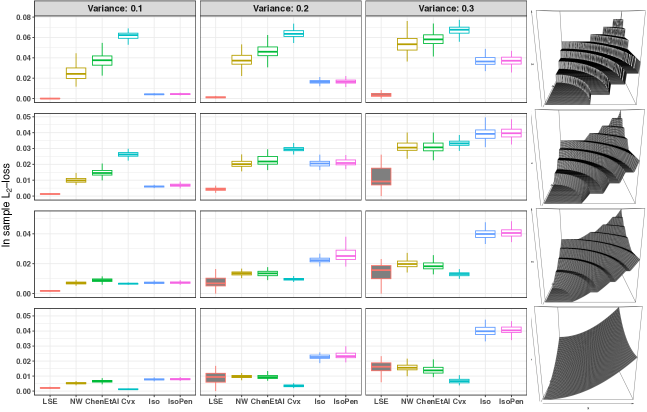
Figure 3: Box plots comparing the performance of our quasiconvex and monotone estimator with other competing estimators in (25) when $n=400$ and $d=2$. The smoothness parameter $\xi$ increases along $0.01,0.34,0.67,1$ as one goes down the rows and error variance increases along $0.1,0.2,0.3$ as one goes from left to right. The rightmost column plots the true conditional mean $\psi_{\xi}$ as $\xi$ increases. The box plots summarize results over 100 replications.

In Figure 3, we show box plots for $\sum_{i=1}^{n}(\widetilde{\varphi}(\boldsymbol{X}_{i})-\varphi(\boldsymbol{X}_{i}))^{2}$ (in sample $L_{2}$-loss) comparing the performance of our quasiconvex and monotone LSE with the other four competing estimators when $d=2$ in (25) with (26). As we go from left to right, the noise variance increases from $0.1$ to $0.3$ in increments of $0.1$. The smoothness parameter $\xi$ increases from $0.01$ to $1$ in increments of $0.33$ as we go from top to bottom in Figure 3. The sample size in each case is taken to be $400$, and the box plots are created over $100$ replications. In each of the settings, the proposed LSE performs significantly better than monotonicity (only) based estimators (Iso and IsoPen). When the true conditional mean is convex, Cvx has the best performance (unsurprisingly). When the true conditional mean function is piecewise constant or the noise variance is low, the LSE has much better performance when compared to shape enforced estimator ChenEtAl. However when the true conditional mean function is smooth (bottom row) and the noise variance is high then both the LSE and the shape enforced estimator ChenEtAl have comparable performance. A similar relationship between the shape enforced operator based on rearrangement and isotonic LSE is observed in the case of univariate monotone regression (Chernozhukov et al.,, 2009, Section 2.4).

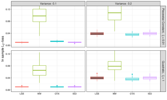
Figure 4: Box plots comparing the in sample $L_{2}(P)$-loss of our proposed LSE with the 3 competing estimators when the true conditional mean function is as defined in (26), with $n=100$, and $d=4$. The box plots summarize results over 100 replications.

Figure 4 deals with (25) when $d=4$. It compares the performance of our quasiconvex and monotone LSE with that of the convexity constrained LSE. The plot provides numerical justification for the optimality of the quasiconvex LSE established in Section 5.1. The sample size is taken to be $100$ and the error variances are allowed to be $0.1$ and $0.2$. In all of the cases in Figure 4, the proposed LSE performs well and its average $L_{2}$ error is close to that of the convex LSE. This is especially remarkable when $\xi=1$, as then the true conditional mean function is convex and convex LSE is minimax optimal in this setting. This reaffirms the remarkable behavior of the quasiconvex LSE that it performs as well as the convex LSE when $d\geq 4$, even when the true conditional mean function is convex.

6.2 Misspecified setting

We also consider regression setup where the true mean is not quasiconvex. We do this by perturbing the functions $\psi_{\xi}$ (defined in (26)) slightly, so that the resulting true conditional mean function is not quasiconvex. To be specific, in Figure 5, we consider the following perturbed version of $\psi_{\xi}$:

$${\psi}^{\dagger}_{\xi}(\boldsymbol{x})=\begin{cases}\lfloor\|\boldsymbol{x}\|_{2}^{2}\rfloor+1&\quad\text{if}~{}\boldsymbol{x}\geq r(\boldsymbol{x}),\\ \psi_{\xi}(\boldsymbol{x})&\quad\text{otherwise},\end{cases}$$ (27)

where

$$r(\boldsymbol{x}):=\begin{cases}\sqrt{\lfloor\|\boldsymbol{x}\|_{2}^{2}\rfloor/2}&\quad\text{if}~{}\|\boldsymbol{x}\|_{2}^{2}\geq 1,\\ \frac{1}{2\sqrt{2}}\left(\sqrt{\lceil\|\boldsymbol{x}\|_{2}^{2}\rceil}+\sqrt{\lfloor\|\boldsymbol{x}\|_{2}^{2}\rfloor}\right)&\quad\text{otherwise}\\ \end{cases}$$

The perturbed function ${\psi}^{\dagger}_{\xi}$ introduces small “bumps” in each step of the piecewise constant function $\psi_{\varepsilon}$ in such a way, that the function is no longer quasiconvex (it continues to be monotone); see the rightmost panel in Figure 5. In each of the $100$ replications the sample size is set to be $400$. As expected, the two monotonicity based estimators outperform all the other estimators in this setting. The proposed quasiconvex and monotone LSE performs reasonably well when compared to the shape enforced estimator ChenEtAl and the convex LSE. The Nadaraya-Watson estimator performs better than both (but worse than the monotonicity based estimators), since it does not assume any shape constraint, and hence is not affected by misspecification from quasiconvexity.

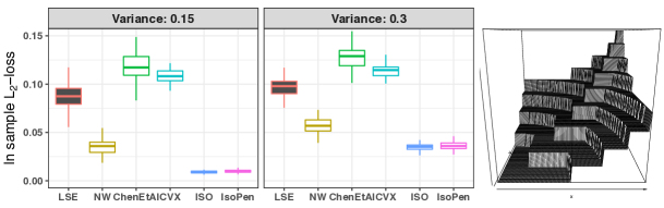
Figure 5: Box plots comparing the performance of the proposed LSE with other competing estimators in the mis-specified setting (27). The sample size is set at $400$ and the number of replications is taken to be 100.

Remark 6.1

Another possible competitor may be tilting based estimators which are viable and important estimators when enforcing various shape constraints. However, currently tilting based estimators can only enforce monotonicity and convex shapes. Du et al., (2013) discuss the enforcement of quasiconcavity only in passing and without any technical details. The codes to compute tilting estimator under monotonicity or convexity were kindly provided to us by Jeffery Racine. However, we did not include them in our simulation due to various technical problems faced by the R package quadprog.

6.3 Numerical Studies under General Covariate Distributions

In Section 6.1, we assumed that the covariates are distributed Uniformly. To better understand the behavior of the LSE under a more complex covariate distribution, we consider:

$$\boldsymbol{X}:=(\psi\cos\eta,\psi\sin\eta)\text{, where}~{}\psi\sim\text{Unif}\,[0,2.5]\text{ and }\eta\sim\text{Unif}\,[0.05,\pi/2-0.05]$$ (28)

This above distribution was used in Yagi et al., (2017) and Olesen and Ruggiero, (2014) to better replicate real data distribution observed in practice. The conditional mean functions considered is the same as the ones in Section 6.1, and we consider the same 4 estimators as in Section 6.1 and compare their performance. The results are summarized in Figure 6.

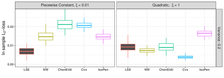
Figure 6: Box plots comparing the in sample $L_{2}(P)$-loss of our proposed LSE with the 4 competing estimators when the true conditional mean function is as defined in (26) and covariate distribution as defined in (28), with $n=400$, and $d=2$. The box plots summarize results over 100 replications.

6.4 Approximate LSE for Large Sample Sizes via Sample Splitting and Minkowski Averaging

While the MIQO formulation (3.6) allows one to compute the LSE for the first time, due to the number of constraints in the computation of the LSE, the memory requirement for the proposed MIQO can make it prohibitive when sample sizes are large ($\gg 500$). In this section, we propose a sample splitting based method to enable approximate computation of the quasiconvex LSE. The sample splitting procedure allows for parallelization of the computation allowing for arbitrarily large sample size. The first step is to split the sample into $K$ splits, one then computes the quasiconvex LSE by applying the MIQO algorithm in Section 3.2 on each of these splits, to compute estimators $\widehat{\varphi}^{(1)},\ldots,\widehat{\varphi}^{(K)}$. The final estimator is then obtained by an aggregation of the above $K$ estimators. In case of the standard non-parametric regression, one can aggregate the estimators by taking a simple pointwise average of the regression function estimates. However, in our case, we need to aggregate the estimators in a way that the resulting estimator is also quasiconvex. Simple averaging doesn’t preserve quasiconvexity as the sum of two quasiconvex functions is not necessarily quasiconvex Volle, (1998). We propose to aggregate the $K$ estimators via the following modified version of infimal convolution (Volle,, 1998) (or level averaging Traoré and Volle, (1996)). We define the aggregate function as:

$$x\mapsto\widehat{\varphi}(\boldsymbol{x}):=\inf\big{\{}\vee_{i=1}^{K}\widehat{\varphi}^{(i)}(\boldsymbol{x}_{i}):K^{-1}\sum_{i=1}^{K}\boldsymbol{x}_{i}=\boldsymbol{x}\big{\}}.$$ (29)

In Lemma C.4 (Section C of the supplement), we show that for every $\alpha\in\mathbb{R}$,

$$\widehat{\varphi}^{-1}((-\infty,\alpha])=\frac{1}{K}\sum_{i=1}^{K}\widehat{\varphi}^{(i)~{}-1}((-\infty,\alpha]),$$

where for sets $A$ and $B$ and $\alpha\in[0,1]$, we define their Minkowski average as: $\alpha A+(1-\alpha)B:=\{\alpha a+(1-\alpha)b:a\in A,b\in B\}.$ The quasiconvexity of $\widehat{\varphi}$ follows immediately from the fact that Minkowski sums (and averages) of convex sets are convex (Krein and Smulian,, 1940). Finally, one can easily show that the $\widehat{\varphi}$ is consistent for $\varphi$ under assumptions discussed in Section 5.

We have added this new estimator to our existing R package QuasiLSE (Mukherjee and Patra,, 2021). We now provide a small simulation to show that the above aggregation works well in practice for larger sample sizes. We implement the new algorithm on a data consisting of $2,000$ bi-variate samples simulated from $\mathrm{Uniform}[0.5,1.5]^{2}$. The regression functions are exactly same as those in Section 6.1, and we fix the error variance at $0.2$, whereas the smoothness parameter $\xi$ is fixed at $0.34$. The entire sample is split into $5$ equal parts, followed by applying the MIQO algorithm (3.6) on each of these splits, and combining the resulting estimators by Minkowski averaging to get the final estimator, plotted in Fig 7 and 8. We see that the Minknowski-aggregated LSE approximates the true function surface very well.

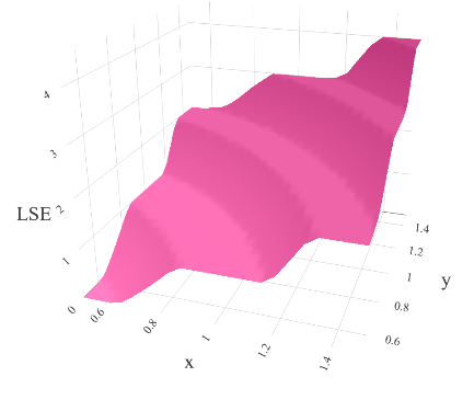
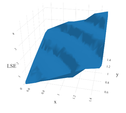
Figure 7: The left panel shows the true function surface and the right panel shows the Minkowski-aggregated LSE surface.

Figure 8: Simultaneous plot showing the true function surface and the Minkowski-aggregated LSE surface. The pink surface denotes the true function, the blue surface denotes the LSE estimate obtained by aggregation through Minkowski averaging.

7 Analysis of the Japanese plywood production data

Foster et al., (2008) studied the production surface in the US plywood industry. Their goal was to predict the value added by a company based on two input variables: Total Employees and Assets. In this section, we consider the production data of $78$ Japanese mid to large plywood factories for the year 2007. To provide a preliminary study of the production surface, in Figure 9, we plot the least squares Cobb-Douglas and the shape enforced (quasiconcave and increasing function) version of the Nadaraya-Watson estimator for the data. The least squares Cobb-Douglas estimate satisfies the economic assumptions of monotonicity and convex input requirement set. Furthermore, this parametric estimator suggests that output for the factories in the data increases by more than the proportional change in inputs. This, however, is inconsistent with the common understanding of microeconomic theory, as the production data contains a mixture of young and mature factories (List and Zhou,, 2007; Haltiwanger et al.,, 2016). “Young” factories generally exhibit increasing returns to scale, while “mature” factories exhibit decreasing returns to scale; see Arrow, (1971) and as there is a mix of young and mature factories in the data, other shape constrained estimators such as concave or $S$-shape estimators will impose additional unjustified structure on the estimator.

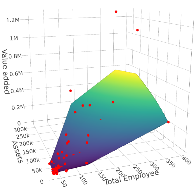
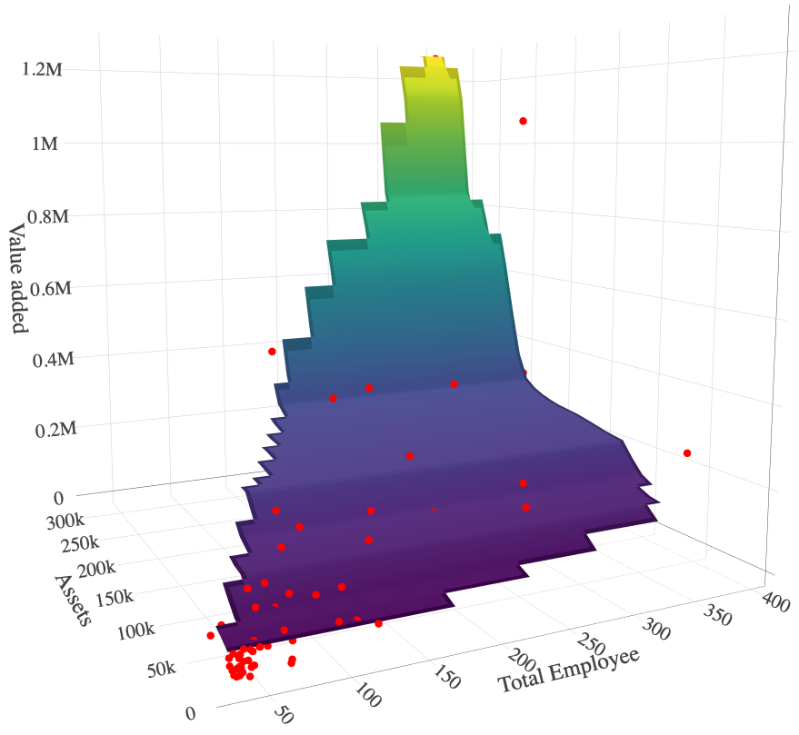
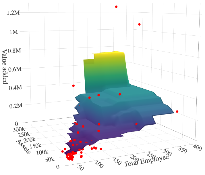
Figure 9: Production surface estimates for the Japanese plywood industry for the year 2007; Left panel: least squares Cobb-Douglas estimate; Middle panel: shape enforced version (ChenEtAl) of the Nadaraya-Watson estimate with bandwidth chosen through least squares cross validation (Li and Racine,, 2007, Page 69) using the np package in R (Hayfield and Racine,, 2008); Right panel: the penalized isotonic regression spline estimator proposed in Meyer, (2013).

We now elaborate on the Japanese production data introduced above, and apply the developed methodology to estimate the production and cost functions. The Japanese plywood data is part of a larger dataset collected by the Japanese Ministry of Economy, Trade, and Industry. The dataset contains production data for various Japanese industries. Japanese industry data is considered to be of high quality for the following reasons: (1) Japan has a large and developed manufacturing industry; (2) Japanese economy was stable during the data collection period; (3) The work practices of the Japanese census are known to be set at very high standards. The above factors result in a high-quality dataset compared to many other countries (Japan’s Ministry of Economy, Trade, and Industry,, 2010). In this paper, we study the 2007 cross-sectional dataset. Foster et al., (2008) argue that plywood production data is particularly suitable for production function estimation using cross establishment data, as plywood establishments produce physically homogeneous products. As discussed above, the least squares Cobb-Douglas estimator fails to properly fit the data. The data contains both young and mature establishments as measured by the establishment date. Young and mature establishments are likely to have different returns to scale. However, the Cobb-Douglas estimator can only have either increasing or decreasing returns to scale. Furthermore, as all the establishments operate on a narrow cone of input ratios, the model assumption of $S$-shape is also too restrictive for this data.

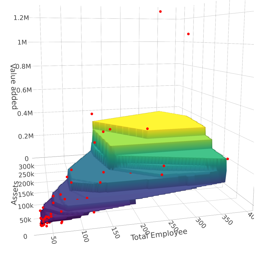
Figure 10: Plot for the Japanese plywood production data from 2007: Left panel – contour plot for the upper level sets for the estimate of the production function; Right Panel – plot of the estimated production function on the convex hull of the observed input variables.

The left panel of Figure 10 shows the input requirement sets for $\widehat{\varphi}_{n}$ and the right panel shows the surface plot of the production function. Notice that as value-added increases, the establishments become more capital intensive. This illustrates the typical pattern of capital deepening as production expands (Kumar and Russell,, 2002). We also observe that establishments are operating at different scales of production throughout the domain of the production function. Our proposed estimator captures the characteristics of the data as flexibly as possible while maintaining the fundamental axioms of monotonicity and quasiconcavity. To further understand the predictive performance of the various estimators discussed in Section 6, we estimate the out-of-sample prediction error by randomly and repeatedly partitioning the data ($100$ times) into 80%/20% training/test splits. The average test error of the competing estimators relative to the LSE is: 1.07 (NW), 1.09 (ChenEtAl), and 1.11 (Iso); the LSE has a relative error of 1 and a lower number is better.

Remark 7.1 (Additional real data example)

In Section A of the supplementary file, we analyze the data of the cost function for hospitals across the US using the 2007 Annual Survey Database from the American Hospital Association studied in Layer et al., (2020). We show that just as in the case of the Japanese production data, existing estimators either overfit or do not adequately incorporate the known shape of the nonparametric function when estimating the cost function.

8 Future work

Several interesting future directions of work follow. The optimal rates of convergence are not known for $d\leq 3$. We plan to study this in the near future. Even though the MIQO developed in Section 3.2 is new, the R package QuasiLSE (Mukherjee and Patra,, 2021) uses CPLEX/gurobi (two off-the-shelf programs) to compute the minimizer. The memory requirement for the proposed MIQO can make it prohibitive when sample sizes are large ($\gg 500$). However, there have been recent developments (see e.g., Dedieu et al., (2020)) that provide approximate solutions to mixed-integer programs. We are currently working towards developing an approximate algorithm that will be computationally less expensive.

9 Acknowledgement

Somabha Mukherjee (SM) and Rohit Kumar Patra (RKP) contributed equally to this work. Hiroshi Morita provided the Japanese plywood production data used in the paper. RKP is the senior statistics author and a bulk of the work was done when SM was a PhD student at the University of Pennsylvania. We thank Arun K. Kuchibhotla and Bodhisattva Sen for their helpful discussions throughout the preparation of the manuscript. We also thank the Joint Editor, the Associate Editor, and the two anonymous referees for their careful reading and constructive comments that led to a much improved paper.

Supplement to “Least Squares Estimation of a Quasiconvex Regression Function”

Summary.  In Section A, we estimate the cost variation across hospitals in the US to illustrate the usefulness of the proposed estimator. Section B reviews some basic concepts and definitions from economics, with the aim of providing a background behind the assumptions for the shapes of the production and cost functions. In Section C, we prove some technical results, that are used throughout the paper. The proofs of Lemma 3.2, Theorem 3.3, Lemma 3.5, and Lemma 3.6 are given in Sections D, E, G, and H, respectively. The validity of Algorithm 1 is established in Section F.

Appendix A Analysis of Hospital cost data

In this section, we analyze the cost variation across hospitals in the US. The analyzed data is from the American Hospital Association’s Annual Survey Database for 2007. The reported cost includes payroll, employee benefits, infrastructure depreciation, interest, supply, and other expenses. For every patient at each of the hospitals, all procedures received are recorded via the International Classification of Diseases, Ninth Revision, Clinical Modification (ICD9-CM) codes (Zuckerman et al.,, 1994). Following Pope and Johnson, (2013) and Layer et al., (2020), we map the codes into four categories of procedures, specifically “Minor Diagnostic,” “Minor Therapeutic,” “Major Diagnostic,” and “Major Therapeutic”. Finally, we add up the number of procedures in each of the categories (for every hospital) to construct the hospital specific output variables.

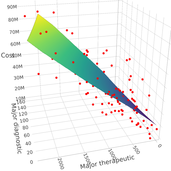
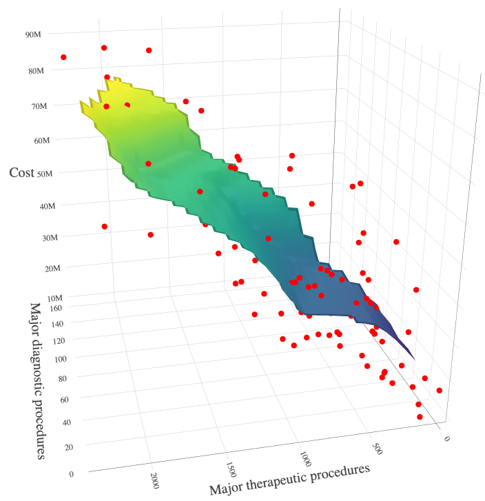
Figure 11: Cost function estimates for the Hospital data on the convex hull of the data for the year 2007. The number of Minor therapeutic and diagnostic procedures are held constant around their median values. Left panel: fit based on a quadratic regression model (without interaction); Right panel: Nadaraya-Watson estimator corrected by ChenEtAl with bandwidth chosen by least squares cross validation using the np package in R.

After some preliminary cleaning up of the data, there are 523 hospitals in our dataset. Layer et al., (2020) conclude that the above four regressors are statistically significant for predicting the cost of the hospitals. However, to keep the results interpretable and be able to plot the cost function, we fix two of the four variables around their median and estimate the two dimensional cost function assuming the two constrained variables to be constant, i.e., we demonstrate the cost function estimator on a “slice” of the data. We consider two different slices of the data. In the first slice, we consider hospitals for which the number of both Minor Therapeutic and Diagnostic procedures are between their respective second and third quartiles; see Figures 11 and 12. The second and third quartiles are chosen so that we have a reasonable amount of the hospitals in the data slice. The estimates in Figures 11 and 12 are based on data from $92$ hospitals. The second slice reverses the role of major and minor procedures and Figure 13 is based on $73$ hospitals.

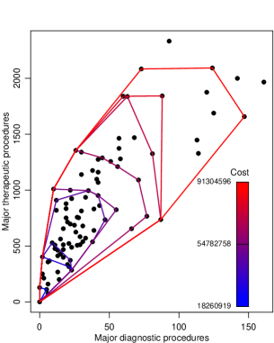
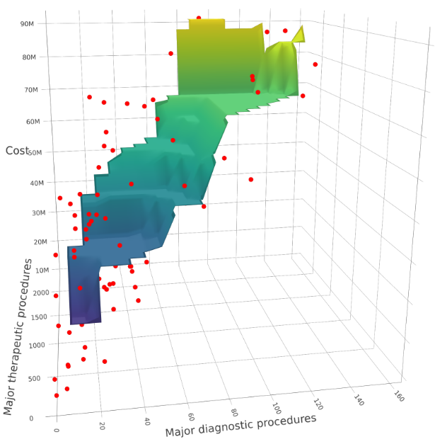
Figure 12: Estimated cost functions when regressing the operating cost of hospitals across the US on the number of major diagnostic and therapeutic procedures, while keeping the number of minor procedures fixed around their median. Left panel: contour plot for the lower level sets for the estimated cost function; Right panel: estimated cost function on the convex hull of the output variables.

In Figure 11, we plot the estimated cost functions using: (1) the fit based on a quadratic model without the interaction term (left panel); and (2) the Nadaraya-Watson estimator with cross-validated choice of the tuning parameter (right panel). A quadratic model (without the cross-product terms) is often used in productivity and efficiency analysis of healthcare data; see e.g., Färe et al., (2010), Layer et al., (2020), and Ferrier et al., (2018). However, in Figure 11, we see that the quadratic cost estimate shows very little substitutability between major therapeutic and major diagnostic procedures in contrast to the nonparametric estimator. On the other hand, the Nadaraya-Watson estimator overfits the data and does not maintain the monotonic structure implied by the standard axioms of the cost function, Shephard, (1970). In Figures 12 and 13, we fit a quasiconvex and increasing function to the two slices of the data. The quasiconvex and increasing LSE is able to estimate a function that characterizes the trade-off between the two outputs for any given cost level, while still maintaining the monotonic structure, implying increasing costs for increasing production, consistent with the basic axioms of production. To further understand the predictive performance of the various estimators discussed in Section 6, we estimate the out-of-sample prediction error by randomly and repeatedly partitioning $100$ times the data into 80%/20% training/test splits. The average test error of the competing estimators relative to the LSE for predicting Major therapeutic and diagnostic procedures is: 0.97 (NW), 0.94 (ChenEtAl), and 3.45 (Iso); and predicting Major therapeutic and diagnostic procedures is: 1.01 (NW), 0.98 (ChenEtAl), and 2.70 (Iso), the LSE has a relative error of 1 and a lower number is better.

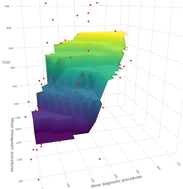
Figure 13: Estimated cost functions when regressing the operating cost of hospitals across the US on the number of minor diagnostic and therapeutic procedures, while keeping the number of major procedures fixed around their median. Left panel: contour plot for the lower level sets of the estimated cost function; Right panel: estimated cost function on the convex hull of the output variables.

Appendix B Economic background and terminologies

In this section, we review some key concepts and definitions from economics. The goal is to provide a basic background behind the assumptions for the characteristics and shapes of the production and cost functions.

Definition B.1 (Return to scale)

A production function $f$ is said to exhibit constant returns to scale, if $f(\lambda\bm{x})=\lambda f(\mathbf{x})$ for all inputs $\bm{x}$ and all $\lambda>0$, increasing returns to scale, if $f(\lambda\bm{x})>\lambda f(\bm{x})$ for all inputs $\mathbf{x}$ and all $\lambda>1$, and decreasing returns to scale, if $f(\lambda\bm{x})<\lambda f(\bm{x})$ for all inputs $\bm{x}$ and all $\lambda>1$ (see (Varian,, 2010, Section 18.10)).

Definition B.2 (Cobb-Douglas production function)

The Cobb-Douglas production function is defined as $F(X_{1},X_{2})=AX_{1}^{\alpha}X_{2}^{\beta}$, where $\alpha,\beta>0$ are the output elasticities of the inputs $X_{1}$ and $X_{2}$, respectively (see (Varian,, 2010, Section 18.3)).

Remark B.3

The Cobb-Douglas production function exhibits constant returns to scale if and only if $\alpha+\beta=1$, increasing returns to scale if and only if $\alpha+\beta>1$, and decreasing returns to scale if and only if $\alpha+\beta<1$.

Appendix C Some technical results

First we introduce some notations and definitions that will be used throughout the rest of the supplement. For a subset $A\in\mathbb{R}^{d}$, $\overline{A}$ denotes the closure of $A$ with respect the Euclidean topology. For two $\otimes_{i=1}^{k}n_{i}$-tensors $\bm{A}$ and $\bm{B}$, the Frobenius inner product of $\bm{A}$ and $\bm{B}$ is defined as:

$$\langle\bm{A},\bm{B}\rangle_{F}:=\sum_{i_{1}=1}^{n_{1}}\ldots\sum_{i_{k}=1}^{n_{k}}A_{i_{1}\ldots i_{k}}B_{i_{1}\ldots i_{k}}\quad\text{and}\quad\|\bm{A}\|_{F}:=\sqrt{\langle\bm{A},\bm{A}\rangle_{F}}.$$ (30)

This section contains some technical lemmas that will be used later.

Lemma C.1

For a convex set $S\subseteq\mathbb{R}^{d}$, the set $S^{\dagger}$ is convex.

Proof C.1.

Take $\bm{Y},\bm{Z}\in S^{\dagger}$ and $\lambda\in[0,1]$. Then, there exist $\bm{W},\bm{X}\in S$, such that $\bm{W}\preccurlyeq\bm{Y}$ and $\bm{X}\preccurlyeq\bm{Z}$. Hence, $\lambda\bm{W}+(1-\lambda)\bm{X}\preccurlyeq\lambda\bm{Y}+(1-\lambda)\bm{Z}$. Now, convexity of the set $S$ implies that $\lambda\bm{W}+(1-\lambda)\bm{X}\in S$, and hence, $\lambda\bm{Y}+(1-\lambda)\bm{Z}\in S^{\dagger}$.

Lemma C.2

For a compact set $S\subseteq\mathbb{R}^{d}$, the set $S^{\dagger}$ is closed.

Proof C.2.

For two sets $S_{1}$ and $S_{2}\subseteq\mathbb{R}^{d}$, if we define $S_{1}+S_{2}:=\{\bm{s}_{1}+\bm{s}_{2}:\bm{s}_{1}\in S_{1},\bm{s}_{2}\in S_{2}\}$, then note that $S^{\dagger}=S+\mathbf{0}_{d}^{\dagger}$. Now, $S$ being compact and $\mathbf{0}_{d}^{\dagger}$ being closed, the result follows.

Lemma C.3

If $\;\widehat{\boldsymbol{\theta}}:=\arg\min_{\boldsymbol{\theta}\in\mathcal{Q}}\|\bm{Y}-\boldsymbol{\theta}\|$, then $\|\widehat{\boldsymbol{\theta}}\|_{\infty}\leq\|\bm{Y}\|_{\infty}$.

Proof C.3.

Suppose, towards a contradiction, that $\|\widehat{\boldsymbol{\theta}}\|_{\infty}>\|\bm{Y}\|_{\infty}$. Define $\boldsymbol{\theta}^{\prime}=(\theta_{1}^{\prime},\ldots,\theta_{n}^{\prime})$ by $\theta_{i}^{\prime}:=\widehat{\theta}_{i}\mathbbm{1}\{|\widehat{\theta}_{i}|\leq\|\bm{Y}\|_{\infty}\}+\mathrm{sgn}(\widehat{\theta_{i}})\|\bm{Y}\|_{\infty}\mathbbm{1}\{|\widehat{\theta}_{i}|>\|\bm{Y}\|_{\infty}\}$. Then, we have:

$$\|\bm{Y}-\boldsymbol{\theta}^{\prime}\|^{2}$$

$$= \sum_{i\,:\,|\widehat{\theta}_{i}|\leq\|\bm{Y}\|_{\infty}}(Y_{i}-\widehat{\theta}_{i})^{2}+\sum_{i\,:\,\widehat{\theta}_{i}>\|\bm{Y}\|_{\infty}}(Y_{i}-\|\bm{Y}\|_{\infty})^{2}+\sum_{i\,:\,\widehat{\theta}_{i}<-\|\bm{Y}\|_{\infty}}(Y_{i}+\|\bm{Y}\|_{\infty})^{2}$$

$$< \sum_{i\,:\,|\widehat{\theta}_{i}|\leq\|\bm{Y}\|_{\infty}}(Y_{i}-\widehat{\theta}_{i})^{2}+\sum_{i\,:\,\widehat{\theta}_{i}>\|\bm{Y}\|_{\infty}}(Y_{i}-\widehat{\theta}_{i})^{2}+\sum_{i\,:\,\widehat{\theta}_{i}<-\|\bm{Y}\|_{\infty}}(Y_{i}-\widehat{\theta}_{i})^{2}=\|\bm{Y}-\widehat{\boldsymbol{\theta}}\|^{2}~{}.$$

Note that the strict inequality above came from the fact that since $\|\widehat{\boldsymbol{\theta}}\|_{\infty}>\|\bm{Y}\|_{\infty}$, i.e., there exists $i$ such that $\widehat{\theta}_{i}>\|\bm{Y}\|_{\infty}$ or $\widehat{\theta}_{i}<-\|\bm{Y}\|_{\infty}$.

We will now show that $\boldsymbol{\theta}^{\prime}\in\mathcal{Q}$, which will yield a contradiction. To this end, suppose $i\in[n]$ and $S\subseteq[n]$ are such that $\bm{X}_{i}\in\textrm{Cv}^{\dagger}\left(\{\bm{X}_{j}:j\in S\}\right)$. By Lemma 3.2, we have $\widehat{\theta}_{i}\leq\max\{\widehat{\theta}_{j}:j\in S\}$. Now, suppose that $|\widehat{\theta}_{i}|\leq\|\bm{Y}\|_{\infty}$. Then, we have:

$$\theta_{i}^{\prime}=\widehat{\theta}_{i}\leq \min\left\{\max\{\widehat{\theta}_{j}:j\in S\},\|\bm{Y}\|_{\infty}\right\}$$

$$= \max\left\{\min\{\widehat{\theta}_{j},\|\bm{Y}\|_{\infty}\}:j\in S\right\}$$

$$\leq \max\{\theta_{j}^{\prime}:j\in S\}~{}.$$

If $\widehat{\theta}_{i}<-\|\bm{Y}\|_{\infty}$, then $\theta_{i}^{\prime}=-\|\bm{Y}\|_{\infty}$, and since $\theta_{j}^{\prime}\geq-\|\bm{Y}\|_{\infty}$ for all $j$, we trivially have $\theta_{i}^{\prime}\leq\max\{\theta_{j}^{\prime}:j\in S\}$. Finally, if $\widehat{\theta}_{i}>\|\bm{Y}\|_{\infty}$, then $\theta_{i}^{\prime}=\|\bm{Y}\|_{\infty}$. But since $\max\{\widehat{\theta}_{j}:j\in S\}\geq\widehat{\theta}_{i}$, there exists $j\in S$ such that $\widehat{\theta}_{j}>\|\bm{Y}\|_{\infty}$, so $\theta_{j}^{\prime}=\|\bm{Y}\|_{\infty}$. Hence, in this case, $\max\{\theta_{j}^{\prime}:j\in S\}=\theta_{i}^{\prime}=\|\bm{Y}\|_{\infty}$. The proof of Lemma C.3 is now complete.

Lemma C.4

In the notations of Section 6.4, for any $\alpha\in\mathbb{R}$, we have:

$$\widehat{\varphi}^{-1}((-\infty,\alpha])=\frac{1}{K}\sum_{i=1}^{K}\widehat{\varphi}^{(i)~{}-1}((-\infty,\alpha]),$$

Proof C.4.

Note that $\boldsymbol{x}\in\widehat{\varphi}^{-1}((-\infty,\alpha])$ if and only if there exists $\boldsymbol{x}_{1},\ldots,\boldsymbol{x}_{K}$ with average $\boldsymbol{x}$, such that $\widehat{\varphi}^{(i)}(\boldsymbol{x}_{i})\leq\alpha$, i.e. $\boldsymbol{x}_{i}\in\widehat{\varphi}^{(i)~{}-1}((-\infty,\alpha])$ for all $i$. The last statement, of course, is equivalent to saying that $\boldsymbol{x}\in\frac{1}{K}\sum_{i=1}^{K}\widehat{\varphi}^{(i)~{}-1}((-\infty,\alpha])$.

Appendix D Proof of Lemma 3.2

Let us define

$$\mathcal{B}:=\bigcap_{(i,S)\in\mathcal{L}{(\mathcal{X})}}\left\{\bm{z}\in\mathbb{R}^{n}:z_{i}\leq\max_{j\in S}z_{j}\right\}~{}.$$

We need to show that $\mathcal{B}=\mathcal{Q}$. First, we show that $\mathcal{Q}\subseteq\mathcal{B}$. To this end, choose $\bm{z}\in\mathcal{Q}$, and let $\psi\in\mathcal{C}$ satisfy $\psi(\bm{X}_{i})=z_{i}$ for all $i\in[n]$. Choose any $(i,S)\in\mathcal{L}(\mathcal{X})$. Then, $\bm{X}_{i}\in\bm{X}^{\dagger}$ for some $\bm{X}\in\mathrm{Cv}\left(\{\bm{X}_{j}:j\in S\}\right)$. Since $\psi$ is decreasing, $\psi(\bm{X}_{i})\leq\psi(\bm{X})$. Since $\psi$ is quasiconvex, $\psi(\bm{X})\leq\max_{j\in S}\psi(\bm{X}_{j})$. Thus, $z_{i}\leq\max_{j\in S}z_{j}$, and hence, $\bm{z}\in\mathcal{B}$, showing that $\mathcal{Q}\subseteq\mathcal{B}$.

Showing the other inclusion is a bit more involved. Choose $\bm{z}\in\mathcal{B}$, and define a function $\bm{z}^{*}:[n]\to[n]$ inductively, as follows. Let $\ell_{1}:=\min\{z_{i}:i\in[n]\}$. Define $\bm{z}^{*}(1):=\min\{i\in[n]:z_{i}=\ell_{1}\}$. Now, assume that $\bm{z}^{*}(1),\ldots,\bm{z}^{*}(m-1)$ have already been defined for some $1<m<n$. Define $\ell_{m}:=\min\{z_{i}:i\in[n]\setminus\{\bm{z}^{*}(1),\ldots,\bm{z}^{*}(m-1)\}\}$ and $\bm{z}^{*}(m):=\min\{i\in[n]\setminus\{\bm{z}^{*}(1),\ldots,\bm{z}^{*}(m-1)\}:z_{i}=\ell_{m}\}$. Clearly,

$$\bm{z}^{*}\text{ is a bijection, and }\bm{z}_{z^{*}(i)}\leq\bm{z}_{z^{*}(j)},\quad\textrm{for all}~{}i<j.$$ (31)

For example, if $n=9$ and $\bm{z}=(4,1,1,6,1,4,6,8,2)$, then $\bm{z}^{*}(1)=2,\bm{z}^{*}(2)=3,\bm{z}^{*}(3)=5,\bm{z}^{*}(4)=9,\bm{z}^{*}(5)=1,\bm{z}^{*}(6)=6,\bm{z}^{*}(7)=4,\bm{z}^{*}(8)=7$ and $\bm{z}^{*}(9)=8$.

Now, define $\psi:\mathbb{R}^{d}\to\mathbb{R}$ inductively, as follows. Set $\psi(\bm{X})=\bm{z}_{\bm{z}^{*}(1)}$ for all $\bm{X}\in\bm{X}_{\bm{z}^{*}(1)}^{\dagger}.$ Suppose inductively, that $\psi$ has been defined on $\mathrm{Cv}^{\dagger}(\{\bm{X}_{\bm{z}^{*}(1)},\ldots,\bm{X}_{\bm{z}^{*}(m-1)}\})$ for some $1<m\leq n$. As the next step, for all $\bm{X}\in\mathrm{Cv}^{\dagger}(\{\bm{X}_{\bm{z}^{*}(1)},\ldots,\bm{X}_{\bm{z}^{*}(m)}\})\setminus\mathrm{Cv}^{\dagger}(\{\bm{X}_{\bm{z}^{*}(1)},\ldots,\bm{X}_{\bm{z}^{*}(m-1)}\})$, define

$$\psi(\bm{X})=\bm{z}_{\bm{z}^{*}(m)}\hskip 2.84544pt.$$

Thus, inductively, $\psi$ is defined on $\mathrm{Cv}^{\dagger}(\{\bm{X}_{\bm{z}^{*}(1)},\ldots,\bm{X}_{\bm{z}^{*}(n)}\})=\mathrm{Cv}^{\dagger}\left(\{\bm{X}_{1},\ldots,\bm{X}_{n}\}\right).$ Finally, define $\psi(\bm{X})=\bm{z}_{\bm{z}^{*}(n)}$ for all $\bm{X}\notin\mathrm{Cv}^{\dagger}\left(\{\bm{X}_{1},\ldots,\bm{X}_{n}\}\right)$.

Several things need to be checked in order, now. First, let us show that $\psi(\bm{X}_{i})=\bm{z}_{i}$ for all $i\in[n]$, or equivalently, that $\psi(\bm{X}_{\bm{z}^{*}(m)})=\bm{z}_{\bm{z}^{*}(m)}$ for all $m\in[n]$. Take an $m\in[n]$, and suppose that $\bm{X}_{\bm{z}^{*}(m)}\in\bm{X}_{\bm{z}^{*}(1)}^{\dagger}$. Since $\bm{z}\in\mathcal{B}$, we must have $\bm{z}_{\bm{z}^{*}(m)}\leq\bm{z}_{\bm{z}^{*}(1)}$. But the reverse inequality is true by (31). Hence, $\psi(\bm{X}_{\bm{z}^{*}(m)})=\bm{z}_{\bm{z}^{*}(1)}=\bm{z}_{\bm{z}^{*}(m)}$. So, assume that $\bm{X}_{\bm{z}^{*}(m)}\notin\bm{X}_{\bm{z}^{*}(1)}^{\dagger}$, whence there exists $1<k\leq m$ such that $\bm{X}_{\bm{z}^{*}(m)}\in\mathrm{Cv}^{\dagger}(\{\bm{X}_{\bm{z}^{*}(1)},\ldots,\bm{X}_{\bm{z}^{*}(k)}\})\setminus\mathrm{Cv}^{\dagger}(\{\bm{X}_{\bm{z}^{*}(1)},\ldots,\bm{X}_{\bm{z}^{*}(k-1)}\})$. Since $\bm{z}\in\mathcal{B}$, we must have $\bm{z}_{\bm{z}^{*}(m)}\leq\bm{z}_{\bm{z}^{*}(k)}$. But the reverse inequality is trivially true; see (31). Hence, $\psi(\bm{X}_{\bm{z}^{*}(m)})=\bm{z}_{\bm{z}^{*}(k)}=\bm{z}_{\bm{z}^{*}(m)}$. This completes our first verification.

Next, we show that the function $\psi$ is decreasing. For this, take $\bm{X}\preccurlyeq\bm{Y}\in\mathbb{R}^{d}$. We need to show that $\psi(\bm{X})\geq\psi(\bm{Y})$. Suppose $\bm{X}\notin\mathrm{Cv}^{\dagger}(\{\bm{X}_{1},\ldots,\bm{X}_{n}\})$, then $\psi(\bm{X})=\bm{z}_{\bm{z}^{*}(n)}$. Since $\psi$ is bounded above by $\bm{z}_{\bm{z}^{*}(n)}$, we are done. Now, suppose that $\bm{X}\in\mathrm{Cv}^{\dagger}(\{\bm{X}_{1},\ldots,\bm{X}_{n}\})$. Let

$$\ell:=\inf\{i\in[n]:\bm{X}\in\mathrm{Cv}^{\dagger}(\{\bm{X}_{\bm{z}^{*}(1)},\ldots,\bm{X}_{\bm{z}^{*}(i)}\})\}.$$

Then, $\psi(\bm{X})=\bm{z}_{\bm{z}^{*}(\ell)}$. Since $\bm{X}\preccurlyeq\bm{Y}$, we must have $\bm{Y}\in\mathrm{Cv}^{\dagger}(\{\bm{X}_{\bm{z}^{*}(1)},\ldots,\bm{X}_{\bm{z}^{*}(\ell)}\})$. Hence, $\psi(\bm{Y})=\bm{z}_{\bm{z}^{*}(k)}$ for some $k\leq\ell$. Since $\bm{z}_{\bm{z}^{*}(k)}\leq\bm{z}_{\bm{z}^{*}(l)}$, our second verification is complete.

Finally, we claim that the function $\psi$ is quasiconvex. Towards showing this, take $\alpha\in\mathbb{R}$. We must show that $S_{\alpha}(\psi)$ is a convex set. If $\alpha<\bm{z}_{\bm{z}^{*}(1)}$, then $S_{\alpha}(\psi)=\emptyset$, whereas if $\alpha\geq\bm{z}_{\bm{z}^{*}(n)}$, then $S_{\alpha}(\psi)=\mathbb{R}^{d}$, and in either case, we are done. So, let us assume that $\bm{z}_{\bm{z}^{*}(1)}\leq\alpha<\bm{z}_{\bm{z}^{*}(n)}$. Then, there exists $k\in[n-1]$ such that $\bm{z}_{\bm{z}^{*}(k)}\leq\alpha<\bm{z}_{\bm{z}^{*}(k+1)}$. Since $\psi(\bm{X})\leq\bm{z}_{\bm{z}^{*}(k)}$ for all $\bm{X}\in\mathrm{Cv}^{\dagger}(\{\bm{X}_{\bm{z}^{*}(1)},\ldots,\bm{X}_{\bm{z}^{*}(k)}\})$, it is clear that $\mathrm{Cv}^{\dagger}(\{\bm{X}_{\bm{z}^{*}(1)},\ldots,\bm{X}_{\bm{z}^{*}(k)}\})\subseteq S_{\alpha}(\psi)$. On the other hand, suppose that $\bm{X}\notin\mathrm{Cv}^{\dagger}(\{\bm{X}_{\bm{z}^{*}(1)},\ldots,\bm{X}_{\bm{z}^{*}(k)}\})$. Then $\psi(\bm{X})=\bm{z}_{\bm{z}^{*}(j)}$ for some $j\geq k+1$, and hence, $\psi(\bm{X})\geq\bm{z}_{\bm{z}^{*}(k+1)}>\alpha$. So, $\bm{X}\notin S_{\alpha}(\psi)$, showing that $S_{\alpha}(\psi)\subseteq\mathrm{Cv}^{\dagger}(\{\bm{X}_{\bm{z}^{*}(1)},\ldots,\bm{X}_{\bm{z}^{*}(k)}\})$. Hence, $S_{\alpha}(\psi)=\mathrm{Cv}^{\dagger}(\{\bm{X}_{\bm{z}^{*}(1)},\ldots,\bm{X}_{\bm{z}^{*}(k)}\})$. Our final claim now follows from Lemma C.1.

We thus conclude that $\mathcal{B}\subseteq\mathcal{Q}$, and the proof of Lemma 3.2 is now complete.

Appendix E Proof of Theorem 3.3

Existence of minimizer: We use the primal characterization of $\mathcal{Q}$ in Lemma 3.2 to prove this. It follows from Lemma 3.2 that the set $\mathcal{Q}$ is a closed set. Let $K:=\mathcal{Q}\cap\overline{B}_{\|\bm{Y}\|+1}\left(\bm{Y}\right)$, where $\bm{Y}:=(Y_{1},\ldots,Y_{n})$. Then, $K$ is nonempty and compact (note that $\mathbf{0}_{n}\in K$). Hence the continuous function $\bm{z}\mapsto\|\bm{Y}-\bm{z}\|$ attains minimum over $K$ at some $\bm{z}_{0}\in K$. For any $\bm{z}\in\mathcal{Q}\setminus\overline{B}_{\|\bm{Y}\|+1}\left(\bm{Y}\right)$, we have $\|\bm{Y}-\bm{z}\|>\|\bm{Y}\|+1>\|\bm{Y}-\bm{z}_{0}\|$, as $\bm{z}_{0}\in\overline{B}_{\|\bm{Y}\|+1}(\bm{Y})$. Hence, the function $\bm{z}\mapsto\|\bm{Y}-\bm{z}\|$ attains minimum over $\mathcal{Q}$ at $\bm{z}_{0}\in\mathcal{Q}$, proving existence of a minimizer of (7).

Almost sure uniqueness of minimizer: Note that the function $d:\mathbb{R}^{n}\to[0,\infty)$ defined by $d(\bm{x},\mathcal{Q}):=\inf\{\|\bm{x}-\boldsymbol{\theta}\|:\boldsymbol{\theta}\in\mathcal{Q}\}$ is Lipschitz on $\mathbb{R}^{n}$. Thus, by Rademacher’s theorem (see Nekvinda and Zajíček, (1988); Alberti and Marchese, (2016)), $x\mapsto d(\bm{x},\mathcal{Q})$ is differentiable Lebesgue almost everywhere on $\mathbb{R}^{n}$. Now, if $d(\bm{x},\mathcal{Q})$ is differentiable at some $\bm{x}\in\mathbb{R}^{n}$, it follows from Majer, (2018) that there exists a unique $\boldsymbol{\theta}\in\mathcal{Q}$ such that $d(\bm{x},\mathcal{Q})=\|\bm{x}-\boldsymbol{\theta}\|$. This shows that the set $\mathcal{K}:=\{\bm{x}\in\mathbb{R}^{n}:d(\bm{x},\mathcal{Q})=\|\bm{x}-\boldsymbol{\theta}\|~{}\textrm{for more than one}~{}\boldsymbol{\theta}\in\mathcal{Q}\}$ has Lebesgue measure $0$. Hence, if $Y$ has density with respect to the Lebesgue measure on $\mathbb{R}$, then so does $\bm{Y}$ with respect to the Lebesgue measure on $\mathbb{R}^{n}$, and hence, $\mathbb{P}(\bm{Y}\in\mathcal{K})=0$. A similar proof can also be found in Keys et al., (2019, Proposition 6).

Appendix F Proof of validity of Algorithm 1

By Lemma 3.2 it is clear that if $\bm{z}\in\mathcal{Q}$, then none of the if statements in Algorithm 1 will be executed, and consequently, the algorithm will always output “out $=1$". On the other hand, suppose that Algorithm 1 outputs “out $=1$". This means that none of the if statements was executed, which in turn, implies that for every $i\in[n]$, $\bm{X}_{i}\notin\mathrm{Cv}^{\dagger}(\{\bm{X}_{j}:z_{j}<z_{i}\})$. Hence, if $\bm{X}_{i}\in\mathrm{Cv}^{\dagger}\left(\{\bm{X}_{j}:j\in S\}\right)$ for some $i\in[n]$ and $S\subseteq[n]$, then $S\nsubseteq\{j\in[n]:z_{j}<z_{i}\}$, which implies that $\max_{j\in S}z_{j}\geq z_{i}$. By Lemma 3.2, we can then conclude that $\bm{z}\in\mathcal{Q}$. This shows the validity of Algorithm 1.

Appendix G Proof of Lemma 3.5

We need a preliminary lemma, to start with.

Lemma G.1

Let $\bm{a},\bm{a}_{1},\ldots,\bm{a}_{k}\in\mathbb{R}^{d}$ be such that $\bm{a}\notin\mathrm{Cv}^{\dagger}(\{\bm{a}_{1},\ldots,\bm{a}_{k}\}).$ Then, there exists $\bm{v}\in\mathbf{0}_{d}^{\dagger}$ , such that $\bm{v}^{\top}(\bm{a}_{i}-\bm{a})>0$ for all $i\in[k].$

Proof G.1.

Define $f:\mathrm{Cv}^{\dagger}(\{\bm{a}_{1},\ldots,\bm{a}_{k}\})\to\mathbb{R}$ as:

$$f(\bm{x})=\|\bm{a}-\bm{x}\|^{2}.$$

Now, since $f$ is a continuous function, it attains minimum on the compact set $\mathrm{Cv}^{\dagger}(\{\bm{a}_{1},\ldots,\bm{a}_{k}\})\bigcap\overline{B}_{\|\bm{a}-\bm{a}_{1}\|}\left(\bm{a}\right)$ at some point $\bm{p}$, where $\overline{B}_{r}(\bm{x})$ denotes the closed $L^{2}$ ball of radius $r$ centered at $\bm{x}$. Clearly, $f(\bm{p})\leq f(\bm{x})$ for all $\bm{x}\in\mathrm{Cv}^{\dagger}(\{\bm{a}_{1},\ldots,\bm{a}_{k}\})$. Take $\bm{v}:=\bm{p}-\bm{a}$ . We first claim that $\bm{v}\in\mathbf{0}_{d}^{\dagger}$. Suppose, towards a contradiction, that $p_{i}<a_{i}$ for some $i\in[d]$. Define $\widetilde{\bm{p}}:=(p_{1},\ldots,p_{i-1},a_{i},p_{i+1},\ldots,p_{d})$. As $\bm{p}\preccurlyeq\widetilde{\bm{p}}$ and $\bm{p}\in\mathrm{Cv}^{\dagger}(\{\bm{a}_{1},\ldots,\bm{a}_{k}\}),$ we have $\widetilde{\bm{p}}\in\mathrm{Cv}^{\dagger}(\{\bm{a}_{1},\ldots,\bm{a}_{k}\})$. However,

$$f(\widetilde{\bm{p}})=f(\bm{p})-(a_{i}-p_{i})^{2}<f(\bm{p})~{},$$

contradicting the minimality of $\bm{p}$ and proving our claim. Next, we show that $\bm{v}^{\top}(\bm{a}_{i}-\bm{a})>0$ for all $i\in[k].$ As $\bm{p}$ is the projection of $\bm{a}$ onto $\mathrm{Cv}^{\dagger}(\{\bm{a}_{1},\ldots,\bm{a}_{k}\})$ (a closed convex set), we have $\langle\bm{p}-\bm{x},\bm{a}-\bm{p}\rangle\geq 0$ for all $\bm{x}\in\mathrm{Cv}^{\dagger}(\{\bm{a}_{1},\ldots,\bm{a}_{k}\})$. Therefore, for any $i\in[k]$,

$$\bm{v}^{\top}(\bm{a}_{i}-\bm{a})=\langle\bm{p}-\bm{a}_{i},\bm{a}-\bm{p}\rangle+\|\bm{p}-\bm{a}\|^{2}\geq\|\bm{p}-\bm{a}\|^{2}>0~{}.$$

Note that the last inequality uses the fact that $\bm{a}\notin\mathrm{Cv}^{\dagger}(\{\bm{a}_{1},\ldots,\bm{a}_{k}\})$ and $\bm{p}\in\mathrm{Cv}^{\dagger}(\{\bm{a}_{1},\ldots,\bm{a}_{k}\})$, so $\bm{a}\neq\bm{p}$. The proof of Lemma G.1 is now complete.

We are now ready to prove Lemma 3.5. Define

$$\mathcal{J}:=\bigcup\limits_{\boldsymbol{\xi}_{1},\ldots,\boldsymbol{\xi}_{n}\in\mathbf{0}_{d}^{\dagger}}\hskip 7.11317pt\bigcap\limits_{(i,j)\in\mathcal{U}(\mathcal{X},\boldsymbol{\xi}_{1},\ldots,\boldsymbol{\xi}_{n})}\{\bm{z}\in\mathbb{R}^{n}:z_{i}\geq z_{j}\}~{},$$

where

$$\mathcal{U}(\mathcal{X},\boldsymbol{\xi}_{1},\ldots,\boldsymbol{\xi}_{n}):=\{(i,j)\in[n]^{2}:\boldsymbol{\xi}_{j}^{\top}(\bm{X}_{i}-\bm{X}_{j})\leq 0\}~{}.$$

Choose $\bm{z}\in\mathcal{J}.$ Then, there exist $\boldsymbol{\xi}_{1},\ldots,\boldsymbol{\xi}_{n}\in\mathbf{0}_{d}^{\dagger}$, such that $z_{i}\geq z_{j}$ for all $i,j\in[n]$ such that $\boldsymbol{\xi}_{j}^{\top}(\bm{X}_{i}-\bm{X}_{j})\leq 0.$ Let $j$ and $S$ be such that $j\in[n],$ $S\subseteq[n]$, and $\bm{X}_{j}\in\mathrm{Cv}^{\dagger}\left(\{\bm{X}_{i}:i\in S\}\right)$, i.e., there exists a $\bm{v}\in\mathbf{0}_{d}^{\dagger}$ and a nonnegative sequence $\{\lambda_{i}\}_{i\in S}$ satisfying $\sum_{i\in S}\lambda_{i}=1$, such that $\bm{X}_{j}=\sum_{i\in S}\lambda_{i}\bm{X}_{i}+\bm{v}$. We will now show $z_{j}\leq\max\{z_{i}:i\in S\}$. Suppose, towards a contradiction, that $z_{j}>\max\{z_{i}:i\in S\}$. Then, $\boldsymbol{\xi}_{j}^{\top}(\bm{X}_{i}-\bm{X}_{j})>0$ for all $i\in S$. Hence, $\boldsymbol{\xi}_{j}^{\top}(\lambda_{i}\bm{X}_{i}-\lambda_{i}\bm{X}_{j})\geq 0$ for all $i\in S$. However, $\sum_{i\in S}\boldsymbol{\xi}_{j}^{\top}(\lambda_{i}\bm{X}_{i}-\lambda_{i}\bm{X}_{j})=-\boldsymbol{\xi}_{j}^{\top}\bm{v}\leq 0$, and hence, $\boldsymbol{\xi}_{j}^{\top}(\lambda_{i}\bm{X}_{i}-\lambda_{i}\bm{X}_{j})=0$ for all $i\in S$. Hence, $\lambda_{i}=0$ for all $i\in S$, contradicting $\sum_{i\in S}\lambda_{i}=1$. So, $z_{j}\leq\max\{z_{i}:i\in S\}$. By Theorem 3.2, $\bm{z}\in\mathcal{Q}$. Hence, $\mathcal{J}\subseteq\mathcal{Q}$.

For showing the reverse inclusion, choose $\bm{z}\in\mathcal{Q}$. Fix $j\in[n]$, and first, suppose that $S_{j}:=\{i\in[n]:z_{i}<z_{j}\}\neq\emptyset.$ By Theorem 3.2, $\bm{X}_{j}\notin\mathrm{Cv}^{\dagger}(\{\bm{X}_{i}:i\in S_{j}\})$. By Lemma G.1, there exists $\boldsymbol{\xi}_{j}\in\mathbf{0}_{d}^{\dagger}$, such that $\boldsymbol{\xi}_{j}^{\top}(\bm{X}_{i}-\bm{X}_{j})>0$ for all $i\in S_{j}$. If $S_{j}=\emptyset$, define $\boldsymbol{\xi}_{j}=\mathbf{0}_{d}$. Thus, we have created $n$ vectors $\boldsymbol{\xi}_{1},\ldots,\boldsymbol{\xi}_{n}\in\mathbf{0}_{d}^{\dagger}$, with the property that whenever $z_{i}<z_{j}$ for some $i,j\in[n]$, we have $\boldsymbol{\xi}_{j}^{\top}(\bm{X}_{i}-\bm{X}_{j})>0$. So, $\bm{z}\in\mathcal{J}$, and hence, $\mathcal{Q}\subseteq\mathcal{J}$, completing the proof of Theorem 3.5.

Appendix H Proof of Lemma 3.6

Note that for every $M>0$ and any feasible solution $(\bm{z}^{\top},\boldsymbol{\xi}_{1}^{\top},\ldots,\boldsymbol{\xi}_{n}^{\top},(u_{ij})_{i\neq j})$ of the MIQO problem (3.6), the vector $\bm{z}$ belongs to $\mathcal{Q}$ by Lemma 3.5. This direction does not need $M$ to be large and holds for any $M$. Now, suppose that $\bm{z}\in\mathcal{Q}$. By Lemma 3.5, there exist vectors $\boldsymbol{\xi}_{1},\ldots,\boldsymbol{\xi}_{n}\in\mathbf{0}_{d}^{\dagger}$ such that $z_{i}\geq z_{j}$ for all $i,j$ satisfying $\boldsymbol{\xi}_{j}^{\top}(\bm{X}_{i}-\bm{X}_{j})\leq 0$. For each $i\neq j$, set

$$u_{ij}=\begin{cases}0&\quad\text{if}\quad\boldsymbol{\xi}_{j}^{\top}(\bm{X}_{i}-\bm{X}_{j})\leq 0,\\ 1&\quad\text{if}\quad\boldsymbol{\xi}_{j}^{\top}(\bm{X}_{i}-\bm{X}_{j})>0.\\ \end{cases}$$

Then, it is easy to check that $(\bm{z}^{\top},\boldsymbol{\xi}_{1}^{\top},\ldots,\boldsymbol{\xi}_{n}^{\top},(u_{ij})_{i\neq j})$ is a feasible solution of the MIQO problem (3.6) whenever $M>\max_{i\neq j}\left\{|z_{i}-z_{j}|\vee\left|\boldsymbol{\xi}_{j}^{\top}(\bm{X}_{i}-\bm{X}_{j})\right|\right\}=:M_{0}$. This is thus the direction, where we need to take $M$ large. The MIQO problem (3.6) is thus indeed equivalent to the problem (7) for all $M>M_{0}$. Lemma 3.6 now follows, by observing that $\mathcal{R}_{M}\subseteq\mathcal{R}_{M+1}$ for all $M\geq 1$.

Appendix I Proof of Theorem 5.1

In the proof of Theorem 5.1, we will use the following standard notations for a function $h:\mathbb{R}^{d}\times R\to\mathbb{R}$:

$$\mathbb{P}_{n}(h):=\frac{1}{n}\sum_{i=1}^{n}h(\bm{X}_{i},Y_{i})\quad\textrm{and}\quad\mathbb{P}(h):=\int_{\mathbb{R}^{d}}h(\bm{X},Y)~{}\mathrm{d}\mathbb{P}(\bm{X},Y)~{}.$$

Finally, we use $C$ to denote a constant. By “constant” we will always mean a quantity that does not depend on $n$ but might depend on the various parameters introduced in our assumptions. In the rest of this paper, we make the convention that the constant $C$ is not necessarily the same on each occurrence.

For any function $h:\mathbb{R}^{d}\to\mathbb{R}$, define

$$\gamma(h,(\bm{X},Y)):=(Y-h(\bm{X}))^{2}.$$ (32)

Recall that $\widehat{\varphi}=\operatorname*{arg\,min}1_{h\in\mathcal{H}_{d,\Gamma}}\mathbb{P}_{n}\gamma(h,\cdot).$ Defining

$$\bar{\varphi}_{\Gamma}:=\operatorname*{arg\,min}1_{h\in\mathcal{H}_{d,\Gamma}}\int_{\mathbb{R}^{d}}\left(h(\bm{x})-\varphi(\bm{x})\right)^{2}~{}\mathrm{d}\mathbb{P}(\bm{x}),$$

we have the following basic inequality $\mathbb{P}_{n}\gamma(\widehat{\varphi},\cdot)\leq\mathbb{P}_{n}\gamma(\bar{\varphi}_{\Gamma},\cdot).$ Finally it follows from $\mathbb{E}(\varepsilon|\bm{X})=0$, that

$$\begin{split}P(\widehat{\varphi}-{\varphi})^{2}&=P(\gamma(\widehat{\varphi},\cdot))-P(\gamma({\varphi},\cdot))\\ &=P(\gamma(\widehat{\varphi},\cdot))-P(\gamma(\bar{\varphi}_{\Gamma},\cdot))+P(\gamma(\bar{\varphi}_{\Gamma},\cdot))-P(\gamma({\varphi},\cdot))\\ &=P(\gamma(\widehat{\varphi},\cdot))-P(\gamma(\bar{\varphi}_{\Gamma},\cdot))+P(\varphi-\bar{\varphi}_{\Gamma})^{2}+\mathbb{P}_{n}\gamma(\bar{\varphi}_{\Gamma},\cdot)-\mathbb{P}_{n}\gamma(\bar{\varphi}_{\Gamma},\cdot)\\ &\leq P(\gamma(\widehat{\varphi},\cdot))-P(\gamma(\bar{\varphi}_{\Gamma},\cdot))+P(\varphi-\bar{\varphi}_{\Gamma})^{2}+\mathbb{P}_{n}\gamma(\bar{\varphi}_{\Gamma},\cdot)-\mathbb{P}_{n}\gamma(\widehat{\varphi},\cdot)\\ &=P(\varphi-\bar{\varphi}_{\Gamma})^{2}+(\mathbb{P}_{n}-P)[\gamma(\bar{\varphi}_{\Gamma},\cdot)-\gamma(\widehat{\varphi},\cdot)]\\ &\leq P(\varphi-\bar{\varphi}_{\Gamma})^{2}+\sup_{h\in\mathcal{H}_{d,\Gamma}}\big{|}(\mathbb{P}_{n}-P)[\gamma(\bar{\varphi}_{\Gamma},\cdot)-\gamma(h,\cdot)]\big{|}.\end{split}$$ (33)

Taking expectation on both sides of the above display, the proof will be complete if we prove:

$$\mathbb{E}\bigg{[}\sup_{h\in\mathcal{H}_{d,\Gamma}}\big{|}(\mathbb{P}_{n}-P)\big{[}\gamma(\bar{\varphi}_{\Gamma},\cdot)-\gamma(h,\cdot)\big{]}\big{|}\bigg{]}$$

$$\leq C\Gamma\max\{\Gamma,C_{\varepsilon},C_{\varphi}\}\times\begin{cases}n^{-1/2}&\text{ when }d=2,\\ n^{-1/2}\log n&\text{ when }d=3,\\ n^{-2/(d+1)}&\text{ when }d\geq 4.\end{cases}$$ (34)

Proof of (I): Observe that

$$\mathbb{E}\bigg{[}\sup_{h\in\mathcal{H}_{d,\Gamma}}\big{|}(\mathbb{P}_{n}-P)\big{[}\gamma(\bar{\varphi}_{\Gamma},\cdot)-\gamma(h,\cdot)\big{]}\big{|}\bigg{]}$$

$$\leq{} \mathbb{E}\bigg{[}\sup_{h\in\mathcal{H}_{d,\Gamma}}\Big{\{}\big{|}(\mathbb{P}_{n}-P)[h-\bar{\varphi}_{\Gamma}]^{2}\big{|}+\big{|}2(\mathbb{P}_{n}-P)[(h-\bar{\varphi}_{\Gamma}(\bm{X}))(Y-\bar{\varphi}_{\Gamma}(\bm{X}))]\big{|}\Big{\}}\bigg{]}$$

$$\leq{} \mathbb{E}\bigg{[}\sup_{h,g\in\mathcal{H}_{d,\Gamma}}\big{|}(\mathbb{P}_{n}-P)[h-g]^{2}\big{|}\bigg{]}+2\mathbb{E}\bigg{[}\sup_{h\in\mathcal{H}_{d,\Gamma}}\Big{|}(\mathbb{P}_{n}-P)\big{[}(h-\bar{\varphi}_{\Gamma})(Y-\bar{\varphi}_{\Gamma})\big{]}\Big{|}\bigg{]}$$

Lemma J.5 provides an upper bound for the first term in (LABEL:eq:proof12.1). We will now bound the second term in (LABEL:eq:proof12.1). Observe that by symmetrization van der Vaart and Wellner, (1996, Lemma 2.3.1)

$$\begin{split}&2\mathbb{E}\bigg{[}\sup_{h\in\mathcal{H}_{d,\Gamma}}\Big{|}(\mathbb{P}_{n}-P)\big{[}(h(\bm{X})-\bar{\varphi}_{\Gamma}(\bm{X}))(Y-\bar{\varphi}_{\Gamma}(\bm{X}))\big{]}\Big{|}\bigg{]}\\ \leq{}&4\mathbb{E}\bigg{[}\sup_{h\in\mathcal{H}_{d,\Gamma}}\Big{|}(\mathbb{P}_{n}-P)\big{[}(Y-\bar{\varphi}_{\Gamma}(\bm{X}))h(\bm{X})\big{]}\Big{|}\bigg{]}\\ \leq{}&4\mathbb{E}\bigg{[}\sup_{h\in\mathcal{H}_{d,\Gamma}}\Big{|}(\mathbb{P}_{n}-P)\big{[}({\varepsilon}+\varphi(\bm{X})-\bar{\varphi}_{\Gamma}(\bm{X}))h(\bm{X})\big{]}\Big{|}\bigg{]}\\ \leq{}&4\mathbb{E}\bigg{[}\sup_{h\in\mathcal{H}_{d,\Gamma}}\Big{|}(\mathbb{P}_{n}-P)\big{[}{\varepsilon}h(\bm{X})\big{]}\Big{|}\bigg{]}+4\mathbb{E}\bigg{[}\sup_{h\in\mathcal{H}_{d,\Gamma}}\Big{|}(\mathbb{P}_{n}-P)\big{[}(\varphi(\bm{X})-\bar{\varphi}_{\Gamma}(\bm{X}))h(\bm{X})\big{]}\Big{|}\bigg{]}\\ ={}&4\mathbb{E}\bigg{[}\sup_{h\in\mathcal{H}_{d,\Gamma}}\Big{|}\mathbb{P}_{n}\big{[}{\varepsilon}h(\bm{X})\big{]}\Big{|}\bigg{]}+4\mathbb{E}\bigg{[}\sup_{h\in\mathcal{H}_{d,\Gamma}}\Big{|}(\mathbb{P}_{n}-P)\big{[}(\varphi(\bm{X})-\bar{\varphi}_{\Gamma}(\bm{X}))h(\bm{X})\big{]}\Big{|}\bigg{]}.\end{split}$$ (36)

Lemma J.4 (see (73) and (74)) provides an upper bound for the both of the above quantities. Combining all this, we get (I).

Appendix J Necessary Lemmas for Section I

Lemma J.1

Let $\mathbb{P}=f(x)dx$ be a probability measure with a continuous density function on $\mathbb{R}^{d}$ such that

$$f(x)\leq C(1+\|x\|)^{-r}\quad\text{ for some }\quad r>(d^{2}+1)/(d-1).$$ (37)

Let $\bm{X}_{1},...,\bm{X}_{n}\sim\mathbb{P}$ be i.i.d. samples from $\mathbb{P}$. Then for any $d\geq 2$ and a fixed positive valued function $m$ such that $\|m\|_{\infty}<\infty$,

$$\mathbb{E}\left[\sup_{K\in\mathcal{K}_{d}}|(\mathbb{P}_{n}-\mathbb{P})[m(\cdot)\mathbf{1}(\cdot\in K)]\right]\leq C_{d}C_{m}n^{-2/(d+1)}\log n^{\mathbf{1}(d=3)},$$ (38)

and

$$\mathbb{E}\left[\sup_{K\in\mathcal{K}_{d}}|(\mathbb{P}_{n}-\mathbb{P})[\varepsilon\mathbf{1}(\cdot\in K)]\right]\leq C_{d}C_{\varepsilon}n^{-2/(d+1)}\log n^{\mathbf{1}(d=3)},$$ (39)

for some constants $C_{m}$, $C_{d}$, and $C_{\varepsilon}$ that depend on $m$, $d$, and $\varepsilon$ only, respectively.

Proof J.1.

We will apply Theorem 2.1 of Han, (2021) to prove the above result. Define

$$\mathcal{G}_{m}:=\{f:\mathbb{R}^{d}\to\mathbb{R}|f(\bm{x})=m(\bm{x})\mathbf{1}(\bm{x}\in K)\text{ for some }K\in\mathcal{K}_{d}\}.$$ (40)

In Lemma J.2, we show that for every $d\geq 2$,

$$\log N_{[]}(\delta,\mathcal{G}_{m},L_{1}(P))\leq C_{d}C_{m}\delta^{-(d-1)/2}.$$ (41)

Then choosing $\sigma^{2}$ in Han, (2021) to be equal to $Pm^{2}$, Theorems 2.1-(2) and  2.3 and Remark 2.4-(2) of Han, (2021) implies that

$$\mathbb{E}\left[\sup_{K\in\mathcal{K}_{d}}\big{|}(\mathbb{P}_{n}-\mathbb{P})[m(\cdot)\mathbf{1}(\cdot\in K)]\big{|}\right] =\mathbb{E}\left[\sup_{f\in\mathcal{G}_{m}}|(\mathbb{P}_{n}-P)f|\right]$$

$$\leq C_{d}C_{m}n^{-2/(d+1)}\log n^{\mathbf{1}(d=3)}.$$ (42)

The proof of (39) is similar. The main difference is, now we choose $\sigma^{2}$ in Theorem 2.1-(2) to be $\mathbb{E}(\varepsilon^{2})$.

Lemma J.2

Let

$$\mathcal{G}_{\varepsilon}:=\{g:\mathbb{R}^{d}\to\mathbb{R}|g(\bm{x})=\varepsilon\mathbf{1}(\bm{x}\in K)\text{ for some }K\in\mathcal{K}_{d}\},$$ (43)

where $\|\mathbb{E}(|\varepsilon|\big{|}\bm{X}=\cdot)\|<\infty$ and for some fixed function $m:\mathbb{R}^{d}\to\mathbb{R}$, let

$$\mathcal{G}_{m}:=\{g:\mathbb{R}^{d}\to\mathbb{R}|g(\bm{x})=m(\bm{x})\mathbf{1}(\bm{x}\in K)\text{ for some }K\in\mathcal{K}_{d}\}.$$ (44)

If $\,P=f(\bm{x})d\bm{x}$ satisfies the assumptions of Lemma J.1, then

$$\log N_{[],1}(\delta,\mathcal{G}_{m},L_{1}(P))\leq C_{d}[\delta/\|m\|_{\infty}]^{-(d-1)/2}$$ (45)

$$\log N_{[],1}(\delta,\mathcal{G}_{\varepsilon},L_{1}(P))\leq C_{d}[\delta/C_{\varepsilon}]^{-(d-1)/2},$$ (46)

where $C_{\varepsilon}:=\big{\|}\mathbb{E}\big{(}|\varepsilon|\big{|}\bm{X}=\cdot)\big{\|}_{\infty}$.

Proof J.2.

We will use the following bound on the bracketing numbers by Bronshtein, (1976) (also Kur et al., (2019, Eq. (33) and Lemma 3) and Dudley, (2014, Theorem 8.4.1)), for every $d\geq 2$ and for every small enough $\epsilon:$

$$\log N_{[],1}(\epsilon,\mathcal{K}_{d}^{(R)},\mathrm{vol})\leq Cd^{(d+4)/2}(\mathrm{vol}B_{d}(0,1))^{(d-1)/2}(\epsilon/R^{d})^{-(d-1)/2},$$ (47)

where for any $R>0$, $\mathcal{K}_{d}^{(R)}$ is the set of convex bodies contained in $B_{d}(0,R)$, the centered Euclidean ball of radius $R.$ As $\mathcal{K}_{d}$ is unbounded, we will partition any set $K\in\mathcal{K}_{d}$ via the following partition for every $i\geq 1$, define $D_{i}=\{x\in\mathbb{R}^{d}:i-1\leq\|x\|\leq i\}.$ Noting that $\cup_{i\geq 1}D_{i}=\mathbb{R}^{d}$, observe that $K=\cup_{i\geq 1}K\cap D_{i}$. Since we can write

$$\begin{split}g(\bm{x})=m(x)\mathbf{1}(\bm{x}\in K)&=\sum_{i\geq 1}m(x)\mathbf{1}(\bm{x}\in K\cap D_{i}):=\sum_{i\geq 1}g_{i}(\bm{x}).\end{split}$$ (48)

and

$$h(\bm{x})=\varepsilon\mathbf{1}(\bm{x}\in K)=\sum_{i\geq 1}\varepsilon\mathbf{1}(\bm{x}\in K\cap D_{i}):=\sum_{i\geq 0}h_{i}(\bm{x}).$$ (49)

Now for each fixed integer $R\geq 1$, let

$$M_{R}:=\sup_{x\in D_{R}}f(x)=CR^{-r}.$$ (50)

Then by observing that for any two sets $A,A^{\prime}\in\mathcal{K}_{d}^{(R)}$, we have $\mathbb{P}(X\in A\Delta A^{\prime})\leq M_{R}\mathrm{vol}(A\Delta A^{\prime})$, we have that

$$\log N_{[],1}(\epsilon,\mathcal{K}_{d}^{(R)},P)\leq\log N_{[],1}(\epsilon/M_{R},\mathcal{K}_{d}^{(R)},\mathrm{vol})\leq C_{d}(\epsilon/M_{R}R^{d})^{-(d-1)/2}=:N(R,\epsilon).$$ (51)

Thus there exist sets $\{(\underaccent{\bar}{S}_{j},\bar{S}_{j})\}_{j=1}^{\exp(N(R,\epsilon))}$ that form an $L_{1}(P)$ bracket for $\mathcal{K}_{d}^{(R)}$, i.e., $\underaccent{\bar}{S}_{j}\subset\bar{S}_{j}$ for every $j\leq N(R,\epsilon)$ and for any set $S\in\mathcal{K}_{d}^{(R)},$ there exists $k\leq\exp(N(R,\epsilon))$ such that $\underaccent{\bar}{S}_{k}\subset S\subset\bar{S}_{k}$ and $P(\bar{S}_{j}\Delta\underaccent{\bar}{S}_{j})\leq\epsilon.$ This implies that

$$\log N_{[],1}(\epsilon,\mathcal{K}_{d}^{(R)}\cap D_{R},P)\leq N(R,\epsilon),$$ (52)

and $\{(\underaccent{\bar}{S}_{j}\cap D_{R},\bar{S}_{j}\cap D_{R})\}_{j=1}^{\exp(N(R,\epsilon))}$ form an $L_{1}(P)$ bracket (of width $\epsilon$) for $\mathcal{K}_{d}^{(R)}\cap D_{R}$, where that for any set of sets $\mathcal{A}$ and a set $B$, $\mathcal{A}\cap B:=\{A\cap B:A\in\mathcal{A}\}.$

Proof of (45): Let $m^{+}(\bm{x}):=\max(0,m(\bm{x}))$ and $m^{-}(\bm{x})=\max(0,-m(\bm{x}))$ define the positive and negative part of $m$, respectively. Defining

$$l_{j,R,\epsilon}:={m^{+}(\cdot)\mathbf{1}\big{(}\cdot\in\underaccent{\bar}{S}_{j}\cap D_{R}\big{)}-m^{-}(\cdot)\mathbf{1}\big{(}\cdot\in\bar{S}_{j}\cap D_{R}\big{)}}$$

and

$$u_{j,R,\epsilon}:={m^{+}(\cdot)\mathbf{1}\big{(}\cdot\in\bar{S}_{j}\cap D_{R}\big{)}-m^{-}(\cdot)\mathbf{1}\big{(}\cdot\in\underaccent{\bar}{S}_{j}\cap D_{R}\big{)}}.$$

We will now show that

$$\Big{\{}\Big{[}{l_{j,R,\epsilon}},{u_{j,R,\epsilon}}\Big{]}\Big{\}}_{j=1}^{\exp(N(R,\epsilon))}$$ (53)

forms an $L_{1}(P)$ bracket (of width $\|m\|_{\infty}\epsilon$) for

$$\mathcal{G}_{m,R}:=\{g:\mathbb{R}^{d}\to\mathbb{R}|g(\bm{x})=m(\bm{x})\mathbf{1}(\bm{x}\in K)\text{ for some }K\in\mathcal{K}_{d}^{R}\cap D_{R}\}.$$

Fix some $S\in\mathcal{K}_{d}^{R}\cap D_{r}$, then by (52), there exists an $k\leq{\exp}(N(R,\epsilon))$ such that $\underaccent{\bar}{S}_{k}\cap D_{R}\subset S\subset\bar{S}_{k}\cap D_{R}$. Thus we have that

$$\begin{split}m^{+}(\cdot)\mathbf{1}\big{(}\cdot\in\underaccent{\bar}{S}_{k}\cap D_{R}\big{)}&\leq m^{+}(\cdot)\mathbf{1}\big{(}\cdot\in{S}\big{)}\leq m^{+}(\cdot)\mathbf{1}\big{(}\cdot\in\bar{S}_{k}\cap D_{R}\big{)},\\ -m^{-}(\cdot)\mathbf{1}\big{(}\cdot\in\bar{S}_{k}\cap D_{R}\big{)}&\leq-m^{-}(\cdot)\mathbf{1}\big{(}\cdot\in{S}\big{)}\leq-m^{-}(\cdot)\mathbf{1}\big{(}\cdot\in\underaccent{\bar}{S}_{k}\cap D_{R}\big{)},\end{split}$$ (54)

Combining the above two inequalities we get that $l_{k,R,\epsilon}\leq m(\cdot)\mathbf{1}\big{(}\cdot\in{S}\big{)}\leq u_{k,R,\epsilon}.$ Thus (60) forms a bracket for $\mathcal{G}_{m,R}$. We will now find the width of this bracket:

$$\begin{split}&P\big{(}\big{|}u_{k,R,\epsilon}-l_{k,R,\epsilon}\big{|}\big{)}\\ ={}&P\bigg{(}\bigg{|}m^{+}(\cdot)\mathbf{1}\big{(}\cdot\in(\bar{S}_{k}\Delta\underaccent{\bar}{S}_{k})\cap D_{R}\big{)}+m^{-}(\cdot)\mathbf{1}\big{(}\cdot\in(\bar{S}_{k}\Delta\underaccent{\bar}{S}_{k})\cap D_{R}\big{)}\bigg{|}\bigg{)}\\ ={}&P\Big{(}|m(\cdot)|\mathbf{1}\big{(}\cdot\in(\bar{S}_{k}\Delta\underaccent{\bar}{S}_{k})\cap D_{R}\big{)}\Big{)}\\ ={}&\|m\|_{\infty}\mathbb{P}\big{(}\bm{X}\in(\bar{S}_{k}\Delta\underaccent{\bar}{S}_{k})\cap D_{R}\big{)}\leq\|m\|_{\infty}\epsilon.\end{split}$$ (55)

Thus we have that

$$\log N_{[],1}(\epsilon,\mathcal{G}_{m,R},P)\leq N(R,\epsilon/\|m\|_{\infty})=C_{d}[\epsilon/(\|m\|_{\infty}M_{R}R^{d})]^{-(d-1)/2}:=Q(m,R,\epsilon),$$ (56)

where $M_{R}$ is defined in (50). We will use the above entropy bound to find an $L_{1}(P)$ bracket for $\mathcal{G}_{m}$ of width $\epsilon$. We will do this by combining $\epsilon_{R}:=\epsilon/(C_{\alpha}R^{\alpha})$ brackets for $\mathcal{G}_{m,R}$ where

$$\alpha:=1+(r-(d^{2}+1)/(d-1))/2,$$ (57)

where $C_{\alpha}:=\sum_{R\geq 1}R^{-\alpha}$; note that $C_{\alpha}<{\infty}$ as $\alpha>1.$ In particular, fix $g\in\mathcal{G}_{m}$, recalling  (48), $g=\sum_{R\geq 1}g_{R}$ ($g_{R}\in\mathcal{G}_{m,R}$). By (56) and (52), we have that there exists $k_{R}\leq\exp(Q(m,R,\epsilon_{R}))$ (see (56)) such that

$$l_{k_{R},R,\epsilon_{R}}\leq g_{R}\leq u_{k_{R},R,\epsilon_{R}},$$

such that $P(|u_{j,R,\epsilon_{R}}-l_{j,R,\epsilon_{R}}|)\leq\epsilon_{R}$, where $\epsilon_{R}=\epsilon/(C_{\alpha}R^{\alpha}).$ Hence it is easy to see that

$$\left\{\Big{[}\sum_{R\geq 1}l_{k_{R},R,\epsilon_{R}},\sum_{R\geq 1}u_{k_{R},R,\epsilon_{R}}\Big{]}\big{|}k_{R}\in[\exp(Q(m,R,\epsilon_{R})]\text{ for every }R\geq 1\right\},$$ (58)

forms an $\epsilon$ bracket for $\mathcal{G}_{m}$ with respect to the $L_{1}(P)$ norm. Thus

$$\begin{split}\log N_{[],1}(\epsilon,\mathcal{G}_{m},P)&\leq\sum_{R\geq 1}Q(m,R,\epsilon_{R})\\ &\leq\sum_{R\geq 1}C_{d}[\epsilon_{R}/(\|m\|_{\infty}M_{R}R^{d})]^{-(d-1)/2}\\ &\leq C_{d}\sum_{R\geq 1}[\epsilon/(C_{\alpha}R^{\alpha}\|m\|_{\infty}M_{R}R^{d})]^{-(d-1)/2}\\ &\leq C_{d}[\epsilon/(\|m\|_{\infty}C_{\alpha})]^{-(d-1)/2}\sum_{R\geq 1}[R^{\alpha}CR^{-r}R^{d}]^{(d-1)/2}\\ &\leq C_{d}[\epsilon/(\|m\|_{\infty}C_{\alpha})]^{-(d-1)/2}\\ &\leq C_{d}[\epsilon/\|m\|_{\infty}]^{-(d-1)/2},\end{split}$$ (59)

as by (37) and (57), we have that $(\alpha+d-r)(d-1)/2<-1.$

Proof of (46): This proof will be similar to the proof of (45) above. Defining $\varepsilon^{+}:=\max(0,\varepsilon)$, $\varepsilon^{-}:=\max(0,-\varepsilon)$,

$$L_{j,R,\epsilon}:={\varepsilon^{+}(\cdot)\mathbf{1}\big{(}\cdot\in\underaccent{\bar}{S}_{j}\cap D_{R}\big{)}-\varepsilon^{-}(\cdot)\mathbf{1}\big{(}\cdot\in\bar{S}_{j}\cap D_{R}\big{)}}$$

and

$$U_{j,R,\epsilon}:={\varepsilon^{+}(\cdot)\mathbf{1}\big{(}\cdot\in\bar{S}_{j}\cap D_{R}\big{)}-\varepsilon^{-}(\cdot)\mathbf{1}\big{(}\cdot\in\underaccent{\bar}{S}_{j}\cap D_{R}\big{)}}.$$

We will now show that

$$\Big{\{}\Big{[}{L_{j,R,\epsilon}},{U_{j,R,\epsilon}}\Big{]}\Big{\}}_{j=1}^{\exp(N(R,\epsilon))}$$ (60)

forms an $L_{1}(P)$ bracket of width $C_{\varepsilon}\epsilon$ (see Lemma J.2 for a definition) for

$$\mathcal{G}_{\varepsilon,R}:=\{g:\mathbb{R}^{d}\to\mathbb{R}|g(\bm{x})=\varepsilon\mathbf{1}(\bm{x}\in K)\text{ for some }K\in\mathcal{K}_{d}^{R}\cap D_{R}\}.$$

Following arguments similar to (54), we see that (60) form a valid bracket. We will now find its width (wrt $L_{1}(P)$ norm).

$$\begin{split}&P\big{(}\big{|}U_{k,R,\epsilon}-L_{k,R,\epsilon}\big{|}\big{)}\\ ={}&P\bigg{(}\bigg{|}\varepsilon^{+}(\cdot)\mathbf{1}\big{(}\cdot\in(\bar{S}_{k}\Delta\underaccent{\bar}{S}_{k})\cap D_{R}\big{)}+\varepsilon^{-}(\cdot)\mathbf{1}\big{(}\cdot\in(\bar{S}_{k}\Delta\underaccent{\bar}{S}_{k})\cap D_{R}\big{)}\bigg{|}\bigg{)}\\ ={}&P\Big{(}|\varepsilon|\mathbf{1}\big{(}\cdot\in(\bar{S}_{k}\Delta\underaccent{\bar}{S}_{k})\cap D_{R}\big{)}\Big{)}\\ ={}&P\Big{(}\mathbb{E}\big{(}|\varepsilon|\big{|}\cdot\big{)}\mathbf{1}\big{(}\cdot\in(\bar{S}_{k}\Delta\underaccent{\bar}{S}_{k})\cap D_{R}\big{)}\Big{)}\\ \leq{}&C_{\varepsilon}P\Big{(}\bar{S}_{k}\Delta\underaccent{\bar}{S}_{k})\cap D_{R}\Big{)},\end{split}$$ (61)

where $C_{\varepsilon}:=\big{\|}\mathbb{E}\big{(}|\varepsilon|\big{|}\bm{X}=\cdot)\big{\|}_{\infty}.$ Thus similar to (56), we have that

$$\log N_{[],1}(\epsilon,\mathcal{G}_{\varepsilon,R},P)\leq N(R,\epsilon/C_{\varepsilon})=C_{d}[\epsilon/(C_{\varepsilon}M_{R}R^{d})]^{-(d-1)/2}:=Q_{\varepsilon}(m,R,\epsilon).$$ (62)

Thus just as in (58), we have that

$$\left\{\Big{[}\sum_{R\geq 1}L_{k_{R},R,\epsilon_{R}},\sum_{R\geq 1}U_{k_{R},R,\epsilon_{R}}\Big{]}\big{|}k_{R}\in[\exp(Q_{\varepsilon}(m,R,\epsilon_{R})]\text{ for every }R\geq 1\right\},$$ (63)

forms an $\epsilon$ bracket for $\mathcal{G}_{\varepsilon}$ wrt to $L_{1}(P)$ norm. Thus

$$\begin{split}\log N_{[],1}(\epsilon,\mathcal{G}_{\varepsilon},P)&\leq\sum_{R\geq 1}Q_{\varepsilon}(m,R,\epsilon_{R})\\ &\leq\sum_{R\geq 1}C_{d}[\epsilon_{R}/(\|m\|_{\infty}M_{R}R^{d})]^{-(d-1)/2}\\ &\leq C_{d}\sum_{R\geq 1}C_{d}[\epsilon/(C_{\alpha}R^{\alpha}C_{\varepsilon}M_{R}R^{d})]^{-(d-1)/2}\\ &\leq C_{d}[\epsilon/(C_{\varepsilon}C_{\alpha})]^{-(d-1)/2}\sum_{R\geq 1}[R^{\alpha}C(1+R)^{-r}R^{d}]^{(d-1)/2}\\ &\leq C_{d}[\epsilon/(C_{\varepsilon}C_{\alpha})]^{-(d-1)/2}\\ &\leq C_{d}[\epsilon/C_{\varepsilon}]^{-(d-1)/2},\end{split}$$ (64)

as by (37) and (57), we have that $(\alpha+d-r)(d-1)/2<-1.$

Lemma J.3 (Lemma 8 of Kur et al., (2019))

Let $\mathcal{H}\subseteq\{h:\mathbb{R}^{d}\mapsto[0,\Gamma]\}$ be a class of non-negative, bounded functions, and let $\mathcal{C}:=\{h^{-1}([0,\alpha]):h\in\mathcal{H},\alpha\in[0,\Gamma]\}$ be the corresponding collection of lower level sets. Then for any fixed function $m(\cdot)$,

$$\mathbb{E}\sup_{h\in\mathcal{H}}\left|\frac{1}{n}\sum_{i=1}^{n}r_{i}m(\bm{X}_{i})h(\bm{X}_{i})\right|$$

$$\leq 2\Gamma\cdot\mathbb{E}\sup_{C\in\mathcal{C}}\big{|}(\mathbb{P}_{n}-P)[m(\cdot)\mathbf{1}(\cdot\in C)]\big{|}+C{\Gamma(\|m\|_{\infty}+\|m\|_{L_{2}(P)})}n^{-1/2}~{},$$ (65)

where $r_{1},\ldots,r_{n}$ are i.i.d. Rademacher random variables and

$$\mathbb{E}\sup_{h\in\mathcal{H}}\Big{|}(\mathbb{P}_{n}-P)\big{[}m(\cdot)h(\cdot)\big{]}\Big{|}\leq\Gamma\,\mathbb{E}\sup_{C\in\mathcal{C}}\big{|}(\mathbb{P}_{n}-P)[m(\cdot)\mathbf{1}(\cdot\in C)]\big{|}+{\Gamma\|m\|_{L_{2}(P)}}n^{-1/2}.$$ (66)

Furthermore,

$$\mathbb{E}\sup_{h\in\mathcal{H}}\Big{|}(\mathbb{P}_{n}-P)\big{[}\varepsilon h(\bm{X})\big{]}\Big{|}\leq\Gamma\,\mathbb{E}\sup_{C\in\mathcal{C}}\big{|}(\mathbb{P}_{n}-P)[\varepsilon\mathbf{1}(X\in C)]\big{|}+\Gamma\mathrm{Var}(\varepsilon)n^{-1/2}.$$ (67)

Proof J.3.

We will first prove (66) and use that to prove (J.3). The reduction scheme here is inspired by Carpenter et al., (2018); also see Han, (2021) and Kur et al., (2019).

Proof of (66): Noting that for $h\in\mathcal{H}$

$$h(\bm{x})=\Gamma-\int_{0}^{\Gamma}\mathbf{1}(h(\bm{x})\leq t)dt,$$

we have

$$\begin{split}&\mathbb{E}\sup_{h\in\mathcal{H}}|\mathbb{P}_{n}(mh)-P(mh)|\\ \ \leq{}&\mathbb{E}\sup_{h\in\mathcal{H}}\left|\int_{0}^{\Gamma}\Big{(}P\big{(}m(\bm{X})\mathbf{1}(h(\bm{X})\leq t)\big{)}-\mathbb{P}_{n}\big{(}m(\bm{X})\mathbf{1}(h(\bm{X})\leq t)\big{)}\Big{)}~{}dt\right|+\Gamma\mathbb{E}\Big{|}(\mathbb{P}_{n}-P)m\Big{|}\\ \ \leq{}&\int_{0}^{\Gamma}\mathbb{E}\sup_{h\in\mathcal{H}}\big{|}(\mathbb{P}_{n}-P)[m(\cdot)\mathbf{1}(h(\bm{X})\leq t)]\big{|}~{}dt+{\Gamma\|m\|_{L_{2}(P)}}n^{-1/2}\\ \ \leq{}&\Gamma\,\mathbb{E}\sup_{h\in\mathcal{H},t\in[0,\Gamma]}\big{|}(\mathbb{P}_{n}-P)[m(\cdot)\mathbf{1}(h(\bm{X})\leq t)]\big{|}+{\Gamma\|m\|_{L_{2}(P)}}n^{-1/2}\\ ={}&\Gamma\,\mathbb{E}\sup_{C\in\mathcal{C}}\big{|}(\mathbb{P}_{n}-P)[m(\cdot)\mathbf{1}(\bm{X}\in C)]\big{|}+{\Gamma\|m\|_{L_{2}(P)}}n^{-1/2}.\end{split}$$ (68)

Proof of (J.3): Observe that

$$\begin{split}&\mathbb{E}\sup_{h\in\mathcal{H}}\left|\frac{1}{n}\sum_{i=1}^{n}r_{i}m(\bm{X}_{i})h(\bm{X}_{i})\right|\\ ={}&\mathbb{E}\sup_{h\in\mathcal{H}}\left|\frac{1}{n}\sum_{i=1}^{n}r_{i}\left(m(\bm{X}_{i})h(\bm{X}_{i})-P(hm)+P(hm)\right)\right|\\ \leq{}&\mathbb{E}\sup_{h\in\mathcal{H}}\left|\frac{1}{n}\sum_{i=1}^{n}r_{i}\left(m(\bm{X}_{i})h(\bm{X}_{i})-P(mh)\right)\right|+\mathbb{E}\sup_{h\in\mathcal{H}}\Big{|}P(mh)\cdot\frac{1}{n}\sum_{i=1}^{n}r_{i}\Big{|}~{}.\end{split}$$ (69)

Let us now bound the two terms in (69). The second term in (69) can be bounded as follows:

$$\mathbb{E}\sup_{h\in\mathcal{H}}\left|P(mh)\cdot\frac{1}{n}\sum_{i=1}^{n}r_{i}\right| \leq \Gamma\|m\|_{\infty}\cdot\mathbb{E}\left|\frac{1}{n}\sum_{i=1}^{n}r_{i}\right|$$

$$\leq \Gamma\|m\|_{\infty}\cdot\sqrt{\mathbb{E}\left[\left(\frac{1}{n}\sum_{i=1}^{n}r_{i}\right)^{2}\right]}=\frac{\Gamma\|m\|_{\infty}}{\sqrt{n}}.$$

For bounding the first term in (69), observing that

$$h(\bm{x})=\Gamma-\int_{0}^{\Gamma}\mathbf{1}(h(\bm{x})\leq t)dt~{},$$

and appealing to the symmetrization lemma (see Lemma 2.3.6 in van der Vaart and Wellner, (1996)), to conclude that:

$$\mathbb{E}\sup_{h\in\mathcal{H}}\left|\frac{1}{n}\sum_{i=1}^{n}r_{i}\left(m(\bm{X}_{i})h(\bm{X}_{i})-P(mh)\right)\right|\leq 2\mathbb{E}\sup_{h\in\mathcal{H}}|\mathbb{P}_{n}(mh)-P(mh)|.$$ (70)

Our result (J.3) now follows from  (68), (69), (J.3) and (70).

Proof of (67): Observe that We will now prove (67). Observe that

$$\begin{split}&\mathbb{E}\sup_{h\in\mathcal{H}}\Big{|}(\mathbb{P}_{n}-P)\big{[}\varepsilon h(\bm{X})\big{]}\Big{|}\\ ={}&\mathbb{E}\sup_{h\in\mathcal{H}}\left|\int_{0}^{\Gamma}\Big{(}P\big{(}\varepsilon\mathbf{1}(h(\bm{X})\leq t)\big{)}-\mathbb{P}_{n}\big{(}\varepsilon\mathbf{1}(h(\bm{X})\leq t)\big{)}\Big{)}~{}dt\right|+\Gamma\mathbb{E}\Big{|}(\mathbb{P}_{n}-P)\varepsilon\Big{|}\\ \leq{}&\int_{0}^{\Gamma}\mathbb{E}\sup_{h\in\mathcal{H}}\big{|}(\mathbb{P}_{n}-P)[\varepsilon\mathbf{1}(h(\bm{X})\leq t)]\big{|}~{}dt+\Gamma\mathrm{Var}(\varepsilon)n^{-1/2}\\ \leq{}&\Gamma\,\mathbb{E}\sup_{h\in\mathcal{H},t\in[0,\Gamma]}\big{|}(\mathbb{P}_{n}-P)[\varepsilon\mathbf{1}(h(\bm{X})\leq t)]\big{|}+\Gamma\mathrm{Var}(\varepsilon)n^{-1/2}\\ ={}&\Gamma\,\mathbb{E}\sup_{C\in\mathcal{C}}\big{|}(\mathbb{P}_{n}-P)[\varepsilon\mathbf{1}(\bm{X}\in C)]\big{|}+\Gamma\mathrm{Var}(\varepsilon)n^{-1/2}.\end{split}$$ (71)

Lemma J.4

Assume that $d\geq 2$. Suppose that $\varepsilon$ has a $2+\delta$ moment bounded by $L$ for some $\delta>0$, and also assume that $\,P=f(\bm{x})d\bm{x}$ satisfies the assumptions of Lemma J.1, then

$$\mathbb{E}\bigg{[}\sup_{h\in\mathcal{H}_{d,\Gamma}}\Big{|}\mathbb{P}_{n}\big{[}rh(\cdot)\big{]}\Big{|}\bigg{]}\leq CC_{d}\Gamma\times\begin{cases}n^{-1/2}&\text{ when }d=2,\\ n^{-1/2}\log n&\text{ when }d=3,\\ n^{-2/(d+1)}&\text{ when }d\geq 4,\end{cases}$$ (72)

$$\mathbb{E}\bigg{[}\sup_{h\in\mathcal{H}_{d,\Gamma}}\Big{|}\mathbb{P}_{n}\big{[}\varepsilon h(\cdot)\big{]}\Big{|}\bigg{]}\leq CC_{\varepsilon}C_{d}\Gamma\times\begin{cases}n^{-1/2}&\text{ when }d=2,\\ n^{-1/2}\log n&\text{ when }d=3,\\ n^{-2/(d+1)}&\text{ when }d\geq 4,\end{cases}$$ (73)

and

$$\mathbb{E}\bigg{[}\sup_{h\in\mathcal{H}_{d,\Gamma}}\Big{|}(\mathbb{P}_{n}-P)\big{[}(\varphi(\cdot)-\bar{\varphi}_{\Gamma}(\cdot))h(\cdot)\big{]}\Big{|}\bigg{]}\leq CC_{\varphi}C_{d}\Gamma\times\begin{cases}n^{-1/2}&\text{ when }d=2,\\ n^{-1/2}\log n&\text{ when }d=3,\\ n^{-2/(d+1)}&\text{ when }d\geq 4,\end{cases}$$ (74)

where $C_{\varepsilon}:=\|\mathbb{E}(\varepsilon|\bm{X}=\cdot)\|_{\infty}+\mathrm{var}(\varepsilon)$, $C_{\varphi}:=\|\varphi-\bar{\varphi}_{\Gamma}\|_{L_{2}(P)}+\|\varphi(\bm{X}_{i})-\bar{\varphi}_{\Gamma}(\bm{X}_{i})\|_{\infty}$ and $C_{d}$ is a constant depending on $d$ only.

Proof J.4.

Let $\mathcal{H}_{d,\Gamma,1}^{+}$ (resp. $\mathcal{H}_{d,\Gamma,2}^{+}$) denote the set of all non-negative quasiconvex (resp. quasiconcave) functions on $\mathbb{R}^{d}$, bounded by $\Gamma$. Since lower level sets of quasiconvex functions (resp. upper level sets of quasiconcave functions) are convex, by choosing $m(\cdot)\equiv 1$, it follows from (38) (Lemma J.1) and (J.3) (Lemma J.3), that for $j\in\{1,2\}$,

$$\mathbb{E}\sup_{h\in\mathcal{H}_{d,\Gamma,j}^{+}}\left|\frac{1}{n}\sum_{i=1}^{n}r_{i}h(\bm{X}_{i})\right|\leq C\Gamma n^{-1/2}+\Gamma C_{d}n^{-2/(d+1)}\log n^{\mathbf{1}(d=3)}.$$ (75)

where $r_{1},\ldots,r_{n}$ are i.i.d. Rademacher random variables. Hence, for $d\geq 2$ we have

$$\mathbb{E}\sup_{h\in\mathcal{H}_{d,\Gamma,j}^{+}}\left|\frac{1}{n}\sum_{i=1}^{n}r_{i}h(\bm{X}_{i})\right|\leq C_{d}\Gamma\times\begin{cases}n^{-1/2}&\text{ when }d=2,\\ n^{-1/2}\log n&\text{ when }d=3,\\ n^{-2/(d+1)}&\text{ when }d\geq 4.\end{cases}$$ (76)

Similarly, using (39) (Lemma J.1) and (67) (Lemma J.3), that for $j\in\{1,2\}$, we have

$$\mathbb{E}\sup_{h\in\mathcal{H}_{d,\Gamma,j}^{+}}\left|\frac{1}{n}\sum_{i=1}^{n}\varepsilon_{i}h(\bm{X}_{i})\right|\leq\Gamma\mathrm{var}(\varepsilon)n^{-1/2}+\Gamma C_{\varepsilon}C_{d}n^{-2/(d+1)}\log n^{\mathbf{1}(d=3)}.$$ (77)

Hence, for $d\geq 2$, we have,

$$\mathbb{E}\sup_{h\in\mathcal{H}_{d,\Gamma,j}^{+}}\left|\frac{1}{n}\sum_{i=1}^{n}\varepsilon_{i}h(\bm{X}_{i})\right|\leq C_{d}C_{\varepsilon}\Gamma\times\begin{cases}n^{-1/2}&\text{ when }d=2,\\ n^{-1/2}\log n&\text{ when }d=3,\\ n^{-2/(d+1)}&\text{ when }d\geq 4.\end{cases}$$ (78)

Finally, using (38) (Lemma J.1) and (66) (Lemma J.3), that for $j\in\{1,2\}$, we have

$$\mathbb{E}\sup_{h\in\mathcal{H}_{d,\Gamma,j}^{+}}\left|(\mathbb{P}_{n}-P)[(\varphi(\cdot)-\bar{\varphi}_{\Gamma}(\cdot))h(\cdot)]\right|\leq\Gamma CC_{\varphi}n^{-1/2}+\Gamma C_{\varphi}C_{d}n^{-2/(d+1)}\log n^{\mathbf{1}(d=3)}.$$ (79)

where $C_{\varphi}:=\|\varphi-\bar{\varphi}_{\Gamma}\|_{L_{2}(P)}+\|\varphi(\bm{X}_{i})-\bar{\varphi}_{\Gamma}(\bm{X}_{i})\|_{\infty}$. Hence, for $d\geq 2$, we have,

$$\mathbb{E}\sup_{h\in\mathcal{H}_{d,\Gamma,j}^{+}}\big{|}(\mathbb{P}_{n}-P)[(\varphi(\cdot)-\bar{\varphi}_{\Gamma}(\cdot))h(\cdot)]\big{|}\leq C_{d}C_{\varphi}\Gamma\times\begin{cases}n^{-1/2}&\text{ when }d=2,\\ n^{-1/2}\log n&\text{ when }d=3,\\ n^{-2/(d+1)}&\text{ when }d\geq 4.\end{cases}$$ (80)

To complete the proof of Lemma J.4, we note that for any quasiconvex function $h$, the function $h^{+}:=\max\{h,0\}$ is non-negative, quasiconvex, and the function $h^{-}=\max\{-h,0\}$ is non-negative, quasiconcave. Hence, we have:

$$\begin{split}\mathbb{E}\sup_{h\in\mathcal{H}_{d,\Gamma}}\left|\frac{1}{n}\sum_{i=1}^{n}h(\bm{X}_{i})\varepsilon_{i}\right|&\leq\mathbb{E}\sup_{h\in\mathcal{H}_{d,\Gamma}}\left|\frac{1}{n}\sum_{i=1}^{n}h^{+}(\bm{X}_{i})\varepsilon_{i}\right|+\mathbb{E}\sup_{h\in\mathcal{H}_{d,\Gamma}}\left|\frac{1}{n}\sum_{i=1}^{n}h^{-}(\bm{X}_{i})\varepsilon_{i}\right|\\ &\leq\mathbb{E}\sup_{h\in\mathcal{H}_{d,\Gamma,1}^{+}}\left|\frac{1}{n}\sum_{i=1}^{n}h(\bm{X}_{i})\varepsilon_{i}\right|+\mathbb{E}\sup_{h\in\mathcal{H}_{d,\Gamma,2}^{+}}\left|\frac{1}{n}\sum_{i=1}^{n}h(\bm{X}_{i})\varepsilon_{i}\right|.\end{split}$$ (81)

The results (72), (73), (74) of Lemma J.4 now follows from by combining (81) with (76), (78), and (80), respectively.

Lemma J.5

Assume that $d\geq 2$, and that the distribution $P$ satisfies the assumptions in Lemma J.4. Then,

$$\mathbb{E}\sup_{f,g\in\mathcal{H}_{d,\Gamma}}\left|\mathbb{P}_{n}(f-g)^{2}-P(f-g)^{2}\right|\leq CC_{d}\Gamma^{2}\times\begin{cases}n^{-1/2}&\text{ when }d=2,\\ n^{-1/2}\log n&\text{ when }d=3,\\ n^{-2/(d+1)}&\text{ when }d\geq 4.\end{cases}$$

Proof J.5.

The following proof is a slight modification of Lemma 7 of  Kur et al., (2019). By Theorem 2.1 in Koltchinskii, (2011), we have:

$$\mathbb{E}\sup_{f,g\in\mathcal{H}_{d,\Gamma}}\left|\mathbb{P}_{n}(f-g)^{2}-P(f-g)^{2}\right|\leq 2\mathbb{E}\sup_{f,g\in\mathcal{H}_{d,\Gamma}}\left|\frac{1}{n}\sum_{i=1}^{n}r_{i}(f(\bm{X}_{i})-g(\bm{X}_{i}))^{2}\right|~{},$$ (82)

where $r_{1},\ldots,r_{n}$ are i.i.d. Rademacher. By Corollary 3.2.2 in Giné and Nickl, (2015), the right hand side of (82) can be bounded as follows:

$$\mathbb{E}\sup_{f,g\in\mathcal{H}_{d,\Gamma}}\left|\frac{1}{n}\sum_{i=1}^{n}r_{i}(f(\bm{X}_{i})-g(\bm{X}_{i}))^{2}\right|\leq 4\Gamma\cdot\mathbb{E}\sup_{f,g\in\mathcal{H}_{d,\Gamma}}\left|\frac{1}{n}\sum_{i=1}^{n}r_{i}(f(\bm{X}_{i})-g(\bm{X}_{i}))\right|~{}.$$ (83)

Combining (82) and (83), we have:

$$\mathbb{E}\sup_{f,g\in\mathcal{H}_{d,\Gamma}}\left|\mathbb{P}_{n}(f-g)^{2}-P(f-g)^{2}\right| \leq 8\Gamma\cdot\mathbb{E}\sup_{f,g\in\mathcal{H}_{d,\Gamma}}\left|\frac{1}{n}\sum_{i=1}^{n}r_{i}(f(\bm{X}_{i})-g(\bm{X}_{i}))\right|$$

$$\leq 16\Gamma\cdot\mathbb{E}\sup_{f\in\mathcal{H}_{d,\Gamma}}\left|\frac{1}{n}\sum_{i=1}^{n}r_{i}f(\bm{X}_{i})\right|.$$ (84)

The last inequality in (J.5) follows from the triangle inequality. Lemma J.5 now follows from (J.5), (76), and (81).

References

- Alberti and Marchese, (2016) Alberti, G. and Marchese, A. (2016). On the differentiability of lipschitz functions with respect to measures in the euclidean space. Geometric and Functional Analysis, 26:1–66.
- Arrow, (1971) Arrow, K. J. (1971). The economic implications of learning by doing. In Readings in the Theory of Growth, pages 131–149. Springer.
- (3) Balabdaoui, F., Durot, C., and Jankowski, H. (2019a). Least squares estimation in the monotone single index model. Bernoulli, 25(4B):3276–3310.
- (4) Balabdaoui, F., Groeneboom, P., and Hendrickx, K. (2019b). Score estimation in the monotone single-index model. Scandinavian Journal of Statistics, 46(2):517–544.
- Beattie et al., (1985) Beattie, B. R., Taylor, C. R., and Watts, M. J. (1985). The economics of production. Number 338.5 B369. Wiley New York.
- Bellec, (2018) Bellec, P. C. (2018). Sharp oracle inequalities for least squares estimators in shape restricted regression. The Annals of Statistics, 46(2):745–780.
- Berndt and Christensen, (1973) Berndt, E. R. and Christensen, L. R. (1973). The translog function and the substitution of equipment, structures, and labor in us manufacturing 1929-68. Journal of econometrics, 1(1):81–113.
- Blanchet et al., (2019) Blanchet, J., Glynn, P. W., Yan, J., and Zhou, Z. (2019). Multivariate distributionally robust convex regression under absolute error loss. Advances in Neural Information Processing Systems, 32:11817–11826.
- Bronshtein, (1976) Bronshtein, E. M. (1976). -entropy of convex sets and functions. Siberian Mathematical Journal, 17(3):393–398.
- Brunk, (1969) Brunk, H. (1969). Estimation of Isotonic Regression. Technical report, mathematical sciences. University of Missouri-Columbia.
- Carpenter et al., (2018) Carpenter, T., Diakonikolas, I., Sidiropoulos, A., and Stewart, A. (2018). Near-optimal sample complexity bounds for maximum likelihood estimation of multivariate log-concave densities. In Conference On Learning Theory, pages 1234–1262. PMLR.
- Chambers, (1988) Chambers, R. G. (1988). Applied production analysis: a dual approach. Cambridge University Press.
- Chatterjee et al., (2015) Chatterjee, S., Guntuboyina, A., and Sen, B. (2015). On risk bounds in isotonic and other shape restricted regression problems. The Annals of Statistics, 43(4):1774 – 1800.
- Chazelle, (1993) Chazelle, B. (1993). An optimal convex hull algorithm in any fixed dimension. Discrete & Computational Geometry, 10(4):377–409.
- Chen et al., (2018) Chen, X., Chernozhukov, V., Fernández-Val, I., Kostyshak, S., and Luo, Y. (2018). Shape-enforcing operators for point and interval estimators. arXiv:1809.01038v3.
- Chernozhukov et al., (2009) Chernozhukov, V., Fernandez-Val, I., and Galichon, A. (2009). Improving point and interval estimators of monotone functions by rearrangement. Biometrika, 96(3):559–575.
- Dedieu et al., (2020) Dedieu, A., Hazimeh, H., and Mazumder, R. (2020). Learning sparse classifiers: Continuous and mixed integer optimization perspectives. arXiv:2001.06471.
- Deng and Zhang, (2020) Deng, H. and Zhang, C.-H. (2020). Isotonic regression in multi-dimensional spaces and graphs. The Annals of Statistics, 48(6):3672 – 3698.
- Diewert, (1982) Diewert, W. E. (1982). Duality approaches to microeconomic theory. Handbook of mathematical economics, 2:535–599.
- Du et al., (2013) Du, P., Parmeter, C. F., and Racine, J. S. (2013). Nonparametric kernel regression with multiple predictors and multiple shape constraints. Statistica Sinica, pages 1347–1371.
- Dudley, (2014) Dudley, R. M. (2014). Uniform central limit theorems, volume 142. Cambridge university press.
- Färe et al., (2010) Färe, R., Martins-Filho, C., and Vardanyan, M. (2010). On functional form representation of multi-output production technologies. Journal of Productivity Analysis, 33(2):81–96.
- Ferrier et al., (2018) Ferrier, G. D., Leleu, H., Valdmanis, V. G., and Vardanyan, M. (2018). A directional distance function approach for identifying the input/output status of medical residents. Applied Economics, 50(9):1006–1021.
- Foster et al., (2008) Foster, L., Haltiwanger, J., and Syverson, C. (2008). Reallocation, firm turnover, and efficiency: Selection on productivity or profitability? The American economic review, 98(1):394–425.
- Giné and Nickl, (2015) Giné, E. and Nickl, R. (2015). Mathematical Foundations of Infinite-Dimensional Statistical Models. Cambridge Series in Statistical and Probabilistic Mathematics. Cambridge University Press.
- Haltiwanger et al., (2016) Haltiwanger, J., Jarmin, R. S., Kulick, R. B., and Miranda, J. (2016). High growth young firms: Contribution to job, output and productivity growth. US Census Bureau Center for Economic Studies Paper No. CES-WP-16-49.
- Han, (2021) Han, Q. (2021). Set structured global empirical risk minimizers are rate optimal in general dimensions. arXiv preprint arXiv:1905.12823.
- Han et al., (2019) Han, Q., Wang, T., Chatterjee, S., and Samworth, R. J. (2019). Isotonic regression in general dimensions. The Annals of Statistics, 47(5):2440–2471.
- Han and Wellner, (2016) Han, Q. and Wellner, J. A. (2016). Multivariate convex regression: global risk bounds and adaptation. arXiv preprint arXiv:1601.06844.
- Han and Wellner, (2019) Han, Q. and Wellner, J. A. (2019). Convergence rates of least squares regression estimators with heavy-tailed errors. The Annals of Statistics, 47:2286 – 2319.
- Hayfield and Racine, (2008) Hayfield, T. and Racine, J. S. (2008). Nonparametric econometrics: The np package. Journal of Statistical Software, 27(5).
- Japan’s Ministry of Economy, Trade, and Industry, (2010) Japan’s Ministry of Economy, Trade, and Industry (2010). Census of manufacture - revised report by enterprise 2007. [Online; access 24-February-2020].
- Johnson and Jiang, (2018) Johnson, A. L. and Jiang, D. R. (2018). Shape constraints in economics and operations research. Statistical Science, 33(4):527–546.
- Jorgenson, (2000) Jorgenson, D. W. (2000). Econometrics: Econometric modeling of producer behavior, volume 1. Mit Press.
- Keys et al., (2019) Keys, K. L., Zhou, H., and Lange, K. (2019). Proximal distance algorithms: Theory and practice. Journal of Machine Learning Research, 20(66):1–38.
- Koltchinskii, (2011) Koltchinskii, V. (2011). Oracle Inequalities in Empirical Risk Minimization and Sparse Recovery Problems: Ecole d’Eté de Probabilités de Saint-Flour XXXVIII-2008, volume 2033. Springer Science & Business Media.
- Krein and Smulian, (1940) Krein, M. and Smulian, V. (1940). On regularly convex sets in the space conjugate to a banach space. Annals of Mathematics, pages 556–583.
- Kuchibhotla and Patra, (2021) Kuchibhotla, A. K. and Patra, R. K. (2021). On least squares estimation under heteroscedastic and heavy-tailed errors. The Annals of Statistics, Forthcoming.
- Kuchibhotla et al., (2021) Kuchibhotla, A. K., Patra, R. K., and Sen, B. (2021). Semiparametric efficiency in convexity constrained single index model. Journal of the American Statistical Association, Forthcoming.
- Kumar and Russell, (2002) Kumar, S. and Russell, R. R. (2002). Technological change, technological catch-up, and capital deepening: relative contributions to growth and convergence. American Economic Review, 92(3):527–548.
- Kuosmanen, (2008) Kuosmanen, T. (2008). Representation theorem for convex nonparametric least squares. The Econometrics Journal, 11(2):308–325.
- Kur et al., (2019) Kur, G., Dagan, Y., and Rakhlin, A. (2019). Optimality of maximum likelihood for log-concave density estimation and bounded convex regression. arXiv preprint arXiv:1903.05315.
- Layer et al., (2020) Layer, K., Johnson, A. L., Sickles, R. C., and Ferrier, G. D. (2020). Direction selection in stochastic directional distance functions. European Journal of Operational Research, 280(1):351–364.
- Lecué and Mendelson, (2012) Lecué, G. and Mendelson, S. (2012). General nonexact oracle inequalities for classes with a subexponential envelope. The Annals of Statistics, 40(2):832–860.
- Li and Racine, (2007) Li, Q. and Racine, J. S. (2007). Nonparametric econometrics: theory and practice. Princeton University Press.
- Lim and Glynn, (2012) Lim, E. and Glynn, P. W. (2012). Consistency of multidimensional convex regression. Operations Research, 60(1):196–208.
- List and Zhou, (2007) List, J. A. and Zhou, H. (2007). Internal increasing returns to scale and economic growth. Technical report, National Bureau of Economic Research.
- Majer, (2018) Majer, P. (2018). Distance function to differentiable at implies unique closest point. https://mathoverflow.net/q/299066.
- Mendelson, (2016) Mendelson, S. (2016). Upper bounds on product and multiplier empirical processes. Stochastic Processes and their Applications, 126(12):3652–3680.
- Meyer, (2013) Meyer, M. C. (2013). A simple new algorithm for quadratic programming with applications in statistics. Communications in Statistics-Simulation and Computation, 42(5):1126–1139.
- Meyer, (2014) Meyer, M. C. (2014). isotonic.pen: Penalized Isotonic Regression in one and two dimensions. https://cran.r-project.org/web/packages/isotonic.pen.
- Mukherjee and Patra, (2021) Mukherjee, S. and Patra, R. K. (2021). QuasiLSE: Least squares estimation under quasiconvex/quasiconcave constraint. https://github.com/rohitpatra/QuasiLSE.
- Nekvinda and Zajíček, (1988) Nekvinda, A. and Zajíček, L. (1988). A simple proof of the rademacher theorem. Časopis pro pěstování matematiky, 113(4):337–341.
- Olesen and Ruggiero, (2014) Olesen, O. B. and Ruggiero, J. (2014). Maintaining the regular ultra passum law in data envelopment analysis. European Journal of Operational Research, 235(3):798–809.
- Pope and Johnson, (2013) Pope, B. and Johnson, A. (2013). Returns to scope: a metric for production synergies demonstrated for hospital production. Journal of Productivity Analysis, 40(2):239–250.
- Saha and Guntuboyina, (2020) Saha, S. and Guntuboyina, A. (2020). On the nonparametric maximum likelihood estimator for gaussian location mixture densities with application to gaussian denoising. The Annals of Statistics, 48(2):738–762.
- Seijo and Sen, (2011) Seijo, E. and Sen, B. (2011). Nonparametric least squares estimation of a multivariate convex regression function. The Annals of Statistics, 39(3):1633–1657.
- Shephard, (1953) Shephard, R. W. (1953). Cost and production functions. Naval Research Logistics, 1(2):104–171.
- Shephard, (1970) Shephard, R. W. (1970). Theory of Cost and Production Functions. Princeton University Press.
- Tirole, (1988) Tirole, J. (1988). The theory of industrial organization. MIT press.
- Traoré and Volle, (1996) Traoré, S. and Volle, M. (1996). On the level sum of two convex functions on banach spaces. Journal of Convex Analysis, 3:141–152.
- van der Vaart and Wellner, (1996) van der Vaart, A. W. and Wellner, J. A. (1996). Weak convergence and empirical processes. Springer Ser. Statist. Springer-Verlag, New York. With applications to statistics.
- Varian, (1992) Varian, H. R. (1992). Microeconomic analysis. WW Norton.
- Varian, (2010) Varian, H. R. (2010). Intermediate Microeconomics, a modern approach. Macmillan & Company, eighth edition.
- Volle, (1998) Volle, M. (1998). Duality for the level sum of quasiconvex functions and applications. ESAIM: Control, Optimisation and calculus of variations, 3:329–343.
- Wu et al., (2015) Wu, J., Meyer, M. C., and Opsomer, J. D. (2015). Penalized isotonic regression. Journal of Statistical Planning and Inference, 161:12–24.
- Yagi et al., (2017) Yagi, D., Johnson, A. L., and Morita, H. (2017). Iterative nonparametric s-shape estimation. Texas A&M Working Paper.
- Zhang, (2002) Zhang, C.-H. (2002). Risk bounds in isotonic regression. The Annals of Statistics, 30(2):528–555.
- Zheng and Glynn, (2017) Zheng, Z. and Glynn, P. W. (2017). Fitting continuous piecewise linear poisson intensities via maximum likelihood and least squares. In 2017 Winter Simulation Conference (WSC), pages 1740–1749. IEEE.
- Zuckerman et al., (1994) Zuckerman, S., Hadley, J., and Iezzoni, L. (1994). Measuring hospital efficiency with frontier cost functions. Journal of health economics, 13(3):255–280.