Variational Learning of Individual Survival Distributions

Abstract.

The abundance of modern health data provides many opportunities for the use of machine learning techniques to build better statistical models to improve clinical decision making. Predicting time-to-event distributions, also known as survival analysis, plays a key role in many clinical applications. We introduce a variational time-to-event prediction model, named Variational Survival Inference (VSI), which builds upon recent advances in distribution learning techniques and deep neural networks. VSI addresses the challenges of non-parametric distribution estimation by ($i$) relaxing the restrictive modeling assumptions made in classical models, and ($ii$) efficiently handling the censored observations, i.e., events that occur outside the observation window, all within the variational framework. To validate the effectiveness of our approach, an extensive set of experiments on both synthetic and real-world datasets is carried out, showing improved performance relative to competing solutions.

1. INTRODUCTION

Prediction of event times, also known as survival analysis in the clinical context, is one of the most extensively studied topics in the statistical literature, largely due to its significance in a wide range of clinical and population health applications. It provides a fundamental set of tools to statistically analyze the future behavior of a system, or an individual. In the classical setup, the primary goal of time-to-event modeling is to either characterize the distribution of the occurrence of an event of interest on a population level (Kaplan and Meier, 1958; Kalbfleisch and Prentice, 2011), or more specifically, to estimate a risk score on a subject level (Cox, 1972). In recent years, there has been a surge of interest in the prediction of individualized event time distributions (Yu et al., 2011).

A characteristic feature in the study of time-to-event distributions is the presence of censored instances, which refer to an event that is not reported during the follow-up period of a subject. This can happen, for instance, when a subject drops out during the study (right censoring), including when the study terminates before the event happens (administrative censoring). Unlike many conventional predictive models, where incomplete observations are usually safely ignored, censored observations contain crucial information that should be adequately considered. To efficiently leverage the censored observations, together with the complete observations, a classical treatment is to work with the notion of a hazard function, formally defined as the instantaneous event risk at time $t$, which can be computed by contrasting the event population to the population at risk at a specific time. Estimates can be derived, for instance by optimizing the partial likelihood defined by the relative hazards in the case of the Cox Proportional Hazard model (CoxPH) (Cox, 1972). Alternatively, other work follows the standard Maximal Likelihood Estimation (MLE) framework, where the individual event distribution is a deformed version of some baseline distribution. For example, in the Accelerated Failure Time model (AFT) (Kalbfleisch and Prentice, 2011), covariate effects are assumed to rescale the temporal index of event-time distributions, i.e., they either accelerate or delay event progression. For censored events, their likelihoods are given as the cumulative density after the censoring time (Aalen et al., 2008).

While vastly popular among practitioners, these models have been criticized for a number of reasons, in particular for the assumptions they make, that consequently render them unfit for many modern applications (Wang et al., 2019). For instance, most survival models, including CoxPH and the proportional odds model (Murphy et al., 1997), work under the premise of fixed covariate effects, overlooking individual uncertainty. However, it has been widely recognized that, individual heterogeneity and other sources of variation are common and often time-dependent (Aalen, 1994). In real-world scenarios, these random factors are typically costly to measure, if not impossible to observe. Unfortunately, many models are known to be sensitive to the violation of this fixed effect assumption, raising seriously concerns when deployed in actual practice (Hougaard, 1995).

Alternatively, machine learning techniques have been leveraged to overcome the limitations of standard statistical survival modeling schemes, especially in terms of model flexibility to address the complexity of data. For example, survival trees employed special node-splitting strategies to stratify the population and derive covariate-based survival curves (Bou-Hamad et al., 2011), support vector machines (Khan and Zubek, 2008) and neural networks (Faraggi and Simon, 1995) have been used for more expressive predictors and LASSO-type variants (Zhang and Lu, 2007) simultaneously execute variable selection to boost statistical efficiency. Bayesian statistics has also been explored in the context of model selection (Lisboa et al., 2003), averaging (Raftery, 1995) and imposing prior beliefs (Fard et al., 2016). Recent advances in modern machine learning bring extra traction to the concept of data-driven survival models, an important step toward precision medicine. Prominent examples include direct deep learning extensions of CoxPH (Katzman et al., 2016; Li et al., 2019), accelerated failure time (Chapfuwa et al., 2018) and Bayesian exponential family models (Ranganath et al., 2016). Other efforts include the use of Gaussian Process to capture complex interactions between covariates in relation to event times (Fernández et al., 2016) and competing risks (Alaa and van der Schaar, 2017). It has been argued that direct modeling of the event distribution might be beneficial (Yu et al., 2011), and more recently, adversarial distribution matching has also been considered for survival applications (Chapfuwa et al., 2018) with promising results reported.

In this work we present a principled approach to address the challenges of nonparametric modeling of time-to-event distributions in the presence of censored instances. Our approach, named Variational Survival Inference (VSI), builds upon recent developments in black-box variational inference (Ranganath et al., 2014). It directly targets the estimation of individualized event-time distributions, rather than a risk score that correlates with event ordering. By explicitly accounting for latent variables in its formulation, VSI better accommodates for individual uncertainty. The proposed VSI is a highly scalable and flexible framework without strong assumptions, featuring easy implementation, stable learning, and importantly, it does not rely on ad-hoc regularizers. Our key contributions include: ($i$) a variational formulation of nonparametric time-to-event distribution modeling conditioned on explanatory variables; ($ii$) a cost-effective treatment of censored observations; ($iii$) a thorough discussion on how our modeling choices impact VSI performance, and ($iv$) an empirical validation confirming that the proposed VSI compares favorably to its counterparts on an extensive set of tasks, covering representative synthetic and real-world datasets.

2. BACKGROUND

A dataset for survival analysis is typically composed of a collection of triplets $D=\{Y_{i}=(t_{i},\delta_{i},X_{i})\}_{i=1}^{N}$, where $i$ indexes the subjects involved in the study. For each triplet, $X_{i}\in\mathbb{R}^{p}$ denotes the set of explanatory variables, $t_{i}$ is the observation time and $\delta_{i}$ is the event indicator. To simplify our discussion, we only consider the standard survival setup. This means $\delta_{i}$ is binary with $\delta_{i}=1$ indicating the event of interest happened at $t_{i}$, otherwise $\delta_{i}=0$ corresponds to a censoring event, i.e., no event occurs until $t_{i}$ and the subject is unobserved thereafter. This distinction creates a natural partition of the dataset $D=D_{c}\bigcup D_{e}$, with $D_{c}=\{Y_{i}:\delta_{i}=0\}$ and $D_{e}=\{Y_{i}:\delta_{i}=1\}$ representing the censored and event groups, respectively.

2.1. Statistical survival analysis

In survival analysis, one is interested in characterizing the survival function $S(t)$, defined as the probability that any given subject survives until time $t$. The basic descriptors involved in the discussion of survival analysis are: the cumulative survival density $F(t)=1-S(t)$, the survival density $f(t)=\partial_{t}F(t)$, the hazard function $h(t)=\lim_{\Delta t\rightarrow 0}\frac{P(t\leq T<t+\Delta t|T\geq t)}{\Delta t}$ and the cumulative hazard function $H(t)=\int_{0}^{t}h(s)\text{d}s$. The following expressions are fundamental to survival analysis (Aalen et al., 2008): $S(t)=\exp(-H(t))$ and $f(t)=h(t)S(t)$. Further, we use $S(t|x)$, $f(t|x)$, $F(t|x)$, $h(t|x)$, $H(t|x))$ to denote their individualized (subject-level) counterparts given explanatory variables $x$. All survival models leverage these definitions to derive population-level estimators or subject-level predictive functions, e.g., of risk, $S(t|x)$, or event time, $f(t|x)$.

2.2. Variational inference

For a latent variable model $p_{\theta}(x,z)=p_{\theta}(x|z)p(z)$, we consider $x\in\mathbb{R}^{p}$ as an observation, i.e., data, and $z\in\mathbb{R}^{m}$ as latent variable. The marginal likelihood, given by $p_{\theta}(x)=\int p_{\theta}(x,z)\text{d}z$, typically does not enjoy a closed form expression. To avoid direct numerical estimation of $p_{\theta}(x)$, Variational Inference (VI) optimizes a variational bound to the marginal log-likelihood. The most popular choice is known as the Evidence Lower Bound (ELBO) (Wainwright and Jordan, 2008), given by

(1) $$\text{ELBO}(x)\triangleq\mathbb{E}_{Z\sim q_{\phi}(z|x)}\left[\log\frac{p_{\theta}(x,Z)}{q_{\phi}(Z|x)}\right]\leq\log p_{\theta}(x),$$

where $q_{\phi}(z|x)$ is an approximation to the true (unknown) posterior $p_{\theta}(z|x)$, and the inequality is a direct result of Jensen’s inequality. The variational gap between the ELBO and true $\log$-likelihood is the KL-divergence between posteriors, i.e., $\text{KL}(q_{\phi}(z|x)\parallel p_{\theta}(z|x))=\mathbb{E}_{q_{\phi}(z|x)}[\log q_{\phi}(z|x)-\log p_{\theta}(z|x)]$, which implies the ELBO tightens as $q_{\phi}(z|x)$ approaches the true posterior $p_{\theta}(z|x)$. For estimation, we seek parameters $\theta$ and $\phi$ that maximize the ELBO. At test time, $q_{\phi}(z|x)$ is used for subsequent inference tasks on new data. Given a set of observations $\{x_{i}\}_{i=1}^{N}$ sampled from data distribution $x\sim p_{d}$, maximizing the expected ELBO is also equivalent to minimizing the KL-divergence $\text{KL}(p_{d}\parallel p_{\theta})$ between the empirical and model distributions. When $p_{\theta}(x|z)$ and $q_{\phi}(z|x)$ are specified as neural networks, the resulting architecture is more commonly known as the Variational Auto-Encoder (VAE) (Kingma and Welling, 2013) in the context of computational vision and natural language processing.

3. VARIATIONAL SURVIVAL INFERENCE

Below we detail the construction of the Variational Survival Inference (VSI) model, which results in predictions of the time-to-event distribution $p_{\theta}(t|x)$ given attribute $x$, with the individual uncertainty accounted in the form of a latent variable $z$ whose distribution is estimated under the VI framework. Unlike classical survival models, we do not need to specify a parametric form for the baseline distribution, e.g., the base hazard $h_{0}(t)$ in CoxPH (Cox, 1972) or the base density $p_{0}(t)$ in AFT (Kalbfleisch and Prentice, 2011). Instead, we leverage the power of deep neural networks to amortize the learning of the event time and survival distributions, allowing arbitrary (high-order) interactions between the predictors and survival time to be captured. This overcomes the limitations caused by the restrictive assumptions made in the classical statistical survival analysis frameworks, thus allowing flexible inference of time-to-event distributions.

3.1. Variational bound of observed events

We start the discussion with the simplest scenario, that for which there are no censoring events. Our goal is to maximize the expected $\log$-likelihood $1/N\sum_{i}\log p_{\theta}(t_{i}|X_{i})$. To model the conditional likelihood, we consider a latent variable model of the form $p_{\theta}(t,z|x)$. The unconditional formulation of the ELBO in (1) can be readily generalized to case conditional on event times as

(2) $$\text{ELBO}(t|x)=\mathbb{E}_{Z\sim q_{\phi}(z|x,t)}\left[\log\frac{p_{\theta}(t,Z|x)}{q_{\phi}(Z|x,t)}\right],$$

where $q_{\phi}(z|x,t)$ denotes the conditional posterior approximation to the true (unknown) $p_{\theta}(z|x,t)$.

In particular, we assume a model distribution with the following decomposition

(3) $$p_{\theta}(t,z|x)=p_{\theta}(t|z,x)p_{\theta}(z|x)=p_{\theta}(t|z)p_{\theta}(z|x),$$

which posits that $z$ is a sufficient statistics of $x$ w.r.t. survival time $t$. Another key assumption we make is that, unlike in the standard variational inference model, we have used a learnable inhomogeneous prior $p_{\theta}(z|x)$ for the latent $z$ to replace the standard fixed homogeneous prior $p(z)$. Such covariate-dependent prior formulation allows the model to account for individual variation, thus further helping to close the variational gap (Tomczak and Welling, 2017). Replacing (3) into the ELBO expression in (2) results in the usual likelihood and KL decomposition pair

(4) $$\begin{aligned} \text{ELBO}(t|x)&=\mathbb{E}_{Z\sim q_{\phi}(z|x,t)}\left[\log p_{\theta}(t|Z)\right]\\[10.0pt] &-\text{KL}(q_{\phi}(z|x,t)\parallel p_{\theta}(z|x)),\end{aligned}$$

from which we can see that maximizing the ELBO is equivalent to estimate the parameters of a probabilistic time-to-event model $p_{\theta}(t|z)p_{\theta}(z|x)$ with maximum likelihood such that the inhomogeneous prior $p_{\theta}(z|x)$ matches as well as possible a conditional posterior that explicitly accounts for event times, $q_{\phi}(z|x,t)$. At test time, only $p_{\theta}(z|x)$ will be used to make predictions provided that $t$ is not available during inference.

More specifically, $p_{\theta}(t|z)$, $p_{\theta}(z|x)$ and $q_{\phi}(z|x,t)$ are defined as neural networks

(5) $$\begin{aligned} p_{\theta}(t|z)&={\rm Softmax}(g(z;\theta)),\\ p_{\theta}(z|x)&={\mathcal{N}}(\mu_{p}(x;\theta),\Sigma_{p}(x;\theta)),\\ q_{\phi}(z|x,t)&={\mathcal{N}}(\mu_{q}(x,t;\phi),\Sigma_{q}(x,t;\phi)),\end{aligned}$$

where $p_{\theta}(t|z)$ is represented on a discretized time line (see below for details), $g(z;\theta)$, $\mu_{p}(x;\theta)$, $\Sigma_{p}(x;\theta)$ and $\mu_{q}(x,t;\phi)$, $\Sigma_{q}(x,t;\phi)$ are deep neural nets parameterized by model parameters $\theta$ and variational parameters $\phi$, and ${\mathcal{N}}(\mu,\Sigma)$ denotes the multivariate Gaussian with mean $\mu$ and (diagonal) covariance $\Sigma$. For standard tabular data, we use Multi Layer Perceptrons (MLPs) to specify these functions.

3.2. Variational bound of censored events

Addressing censoring in the formulation is more challenging as this type of partial observation is not subsumed in the conventional VI framework. To address this difficulty, we recall that in likelihood-based survival analysis, the likelihood function for censored observations is given by $\log S_{\theta}(t|x)$, where $S_{\theta}(t|x)$ is the survival function and $t$ is the censoring time. For censored observations $Y$ with $\delta=0$, we do not have the exact event time $t$. This means that we only have partial information of the events, in that the event should happen only after the censoring time $t$.

To derive a tractable objective for censored observations, we first expand $\mathcal{L}_{c}(x,t)=\log S_{\theta}(t|x)$ based on its definition and an application of Fubini’s theorem (Resnick, 2003) and Jensen’s inequality, i.e.,

$$\mathcal{L}_{c}(x,t) =\text{log }S_{\theta}(t|x)=\text{log }\int_{t}^{\infty}p_{\theta}(t|x)dt$$

$$\geq\mathbb{E}_{q_{\phi}(z|t,x)}\left[\text{log }{\frac{p_{\theta}(z|x)}{q_{\phi}(z|t,x)}}+\text{log }S_{\theta}(t|z)\right]$$

$$=\mathbb{E}_{q_{\phi}(z|t,x)}[\text{log }S_{\theta}(t|z)]$$

$$\hskip 42.67912pt-{\rm KL}(q_{\phi}(z|t,x)||p_{\theta}(z|x))$$

$$\triangleq\text{ELBO}_{c}(t|x)$$

where the censored log-likelihood bound $\text{ELBO}_{c}(t|x)$ is only evaluated on $D_{c}$, i.e., the subset of censored observations. See Supplementary Materials for the full derivation of $\text{ELBO}_{c}(t|x)$.

3.3. Implementing VSI

In the current instantiation of the model, we discretize time into $M$ bins spanning the time horizon of the (training) data. This means that (at inference) $t$ is only known up to the time bin it falls into. We note this is not a restrictive assumption as many survival data is only known up to certain temporal accuracy. That said, generalization to continuous observations is fairly straightforward. For datasets that do have a natural discretization, we leave the choice to the user. In this study, we partition the temporal index based on the percentiles of observed event time, while also allowing for an artificial $(M+1)$-th bin to account for event times beyond the full observation window, i.e., events happening after the end-of-study as observed in the training cohort.

Since both $p_{\theta}(z|x)$ and $q_{\phi}(z|x,t)$ are assumed to be Gaussian, the following closed-form expression can be used in the computation of the KL terms above

(6) $$\begin{array}[]{c}{\rm KL}(q_{\phi}(z|x,t)\parallel p_{\theta}(z|x)))=\frac{1}{2}\left\{\text{tr}\left(\Sigma_{p}^{-1}\Sigma_{q}\right)+\right.\\[5.0pt] \hskip 60.00009pt\left.\left(\mu_{p}-\mu_{q}\right)^{T}\Sigma_{p}^{-1}\left(\mu_{p}-\mu_{q}\right)-m+\log\frac{\det(\Sigma_{p})}{\det(\Sigma_{q})}\right\}.\end{array}$$

Following Ranganath et al. (2014), we use diagonal covariance matrices and apply the reparameterization trick to facilitate stable differatiable learning.

In order to compute the term $S_{\theta}(t|x)$, we use discretized time scheme as previously described, and sum up all predicted probabilities subsequent to bin $t$. Note that this can be readily generalized to continuous time models. So long as the cumulative distribution of $p_{\theta}(t|z)$ enjoys a closed form expression, a numerical integration scheme is not necessary to implement VSI.

3.4. Importance-Weighted estimator for likelihood evaluation

For evaluation purposes, we need to be able to compute the model’s log-likelihood for an observation $Y=(x_{i},t_{i},\delta_{i})$, i.e.,

(7) $$\mathcal{L}_{\rm VSI}(x_{i},t_{i};\theta)=\delta_{i}\log p_{\theta}(t_{i}|x_{i})\\ +(1-\delta_{i})\log S_{\theta}(t_{i}|x_{i}).$$

In this study, we use the importance-weighted (IW) estimator (Burda et al., 2015), which provides a tighter bound to the $\log$-likelihood. While more sophisticated alternatives might provide sharper estimates (Neal, 2001), we deem IW estimator sufficient for the scope of this study. Additionally, while the tighter bound can be repurposed for training, it does not necessarily result in improved performance (Rainforth et al., 2018), which we find to be the case in this study.

To obtain a more accurate value of the likelihood, we use the approximate posterior as our proposal, and use the following finite sample estimate

$$\begin{split}\hat{p}_{\theta}(t_{i}|x_{i})&=\int\frac{p_{\theta}(t_{i}|z)p_{\theta}(z|x)}{q_{\phi}(z|t_{i},x)}q_{\phi}(z|t_{i},x)dz\\ &\approx\frac{1}{L}\sum_{l=1}^{L}\frac{p_{\theta}(t_{i}|z_{l})p_{\theta}(z_{l}|x)}{q_{\phi}(z_{l}|t_{i},x)},\end{split}$$

where $L$ is the number of samples. The log-likelihood for the corresponding conditional survival function is

$$\begin{split}\hat{S}_{\theta}(t_{i}|x_{i})&=\int_{t>t_{i}}\int\frac{p_{\theta}(t_{i}|z)p_{\theta}(z|x)}{q_{\phi}(z|t_{i},x)}q_{\phi}(z|t_{i},x)dzdt\\ &\approx\frac{1}{L}\sum_{l=1}^{L}\frac{\int_{t>t_{i}}p_{\theta}(t,z_{l}|x)dt}{q_{\phi}(z_{l}|t_{i},x)}\end{split}$$

Note that by nature of Jensen’s inequality, the resultant estimand will be an under-estimation of the true $\log$-likelihood. As $L$ goes to infinity, the approximated lower bound will converge to the true $\log$-likelihood.

3.5. Making Predictions

Predictive time-to-event distribution During inference, given a new data point with $x_{*}$, according to the generative model $p_{\theta}(t|x_{*})=\int p_{\theta}(t,z|x_{*})dz=\int p_{\theta}(t|z)p_{\theta}(z|x_{*})dz$, where the integration is conducted numerically by Monte Carlo sampling.

Point estimation of time-to-event To better exploit the learned approximated posterior $q_{\phi}(z|x,t)$, we generalize the importance sampling idea and provide a weighted average as time-to-event summary, rather than for instance using a summary statistic such as median or mean. Specifically, consider multiple samples of $t_{*}^{(l)}\sim p_{\theta}(t|x_{*})$, then calculate a weighted average as

(8) $$\begin{array}[]{c}t_{*}=\frac{\sum_{l=1}^{L}w_{*}^{(l)}t_{*}^{(l)}}{\sum_{l=1}^{L}w_{*}^{(l)}},\,w_{*}^{(l)}=\frac{p_{\theta}(z_{l}|x_{*})}{q_{\phi}(z_{l}|t_{*}^{(l)},x_{*})},\\[10.0pt] t_{*}^{(l)}\sim p_{\theta}(t|x_{*}),\,\,\,z_{l}\sim q_{\phi}(z|t_{*}^{(l)},x_{*}).\end{array}$$

In the Supplementary Materials we show that (8) gives better model performance for point-estimate-based evaluation metrics, Concordance Index in particular, compared to other popular summary statistic such as the median of $t_{*}\sim p_{\theta}(t|x_{*})$ with $L$ empirical samples.

4. DISSECTING VSI

In the experiments, we show the effectiveness of the proposed VSI model in recovering underlying time-to-event distributions. To provide additional insight into the differentiating components of the VSI model, we consider two baseline models that partially adopt a VSI design, as detailed below.

VSI without a $q_{\phi}$ arm (VSI-NoQ) In VSI, we use the variational lower bound to maximize the likelihood in survival studies by implicitly forcing the unknown intractable model posterior $p_{\theta}(z|x)$ to be close to the tractable posterior approximation $q_{\phi}(z|x,t)$. Via the KL divergence minimization, such matching allows the model to better account for interactions between covariates $x$ and event times $t$ captured by $q_{\phi}(z|x,t)$ to better inform the construction of the latent representation $z$ via isolating out the individual uncertainty encoded by $p_{\theta}(z|x)$. If we exclude the interaction term $(x,t)$ in $q_{\phi}$ and only make the prediction with $x$, i.e., with the approximate posterior given by $q_{\phi}(z|x)$, through the same stochastic latent representation $z$, then naturally the optimal solution is to equate $q_{\phi}(z|x)$ with the prior $p_{\theta}(z|x)$ . This basically eliminates $q_{\phi}$ from our formulation, and therefore we call this variant VSI-NoQ.

More specifically, without a $q_{\phi}$ arm the model described in Section 3 essentially becomes a feed-forward model with a special stochastic hidden layer $z$. In this case, the model likelihood is given by $p_{\theta}(t|x)=\int p_{\theta}(t,z|x)dz=\int p_{\theta}(t|z)p_{\theta}(z|x)dz$, where $p_{\theta}(t|z)$ and $p_{\theta}(z|x)$ are defined as in (3). Note that the only difference with VSI is the lack of the KL divergence term to match $p_{\theta}(z|x)$ to $q_{\phi}(z|x,t)$. This baseline model (VSI-NoQ) is considered to dissect the impact of excluding complex interaction between covariates and event time when constructing the individualized priors.

Deterministic feed-forward model (MLP) To understand the importance of the stochastic latent representations $z$, we consider a straightforward baseline which directly predicts the event time distribution based on the input $x$, i.e., $p_{\theta}(\cdot|x)=\rm{Softmax}(g_{\theta}(x))$, which is essentially a standard multinomial regression with censored observation. In our study, we use the MLP to implement $g_{\theta}(x)$. And as such, hereafter we will refer to this model as MLP. Additionally, we also considered standard randomization schemes, such as dropout (Srivastava et al., 2014), in the construction of a stochastic neural net, which promises to improve performance. Such strategy also incorporates randomness, however differs principally from the modeled uncertainty exploited by our VSI scheme. In our experiment section, we report the best results from MLP with or without dropout.

These baseline approaches use feed-forward deep learning networks to learn $p_{\theta}(t|x)$ without incurring the notation of variational inference. In the experiments we will show that the variational inference is crucial to the accurate learning of time-to-event distributions, resulting in better performance relative to these baselines, especially when the proportion of censoring events is high.

5. RELATED WORK

Machine learning and survival analysis Early attempts of combining machine learning techniques with statistical survival analysis, such as the Faraggi-Simon network (FS-network) (Faraggi and Simon, 1995), often failed to demonstrate a clear advantage over classical baselines (Schwarzer et al., 2000). Recent progresses in machine learning allow researchers to overcome the difficulties suffered by prior studies. For example, Katzman et al. (2018) showed that weight decay, batch normalization and dropout significantly improved the performance of FS-network. Li et al. (2019) analyzed survival curves based on clinical images using deep convolution neural net (CNN). In addition to deep nets, Fernández et al. (2016) showed that Gaussian Process can be used to effectively capture the non-linear variations in CoxPH models, and Alaa and van der Schaar (2017) further proposed a variant that handles competing risks. Similar to these works, our VSI also draws power from recent advances in machine learning to define a flexible learner.

Bayesian survival analysis Bayesian treatment of survival models has a long history. Raftery et al. (1996) first considered modeling uncertainties for survival data, Zupan et al. (1999) reported probabilistic analysis under Bayesian setup. More recently, Fard et al. (2016) exploited the Bayesian framework to extrapolate priors, and Zhang and Zhou (2018) described a Bayesian treatment of competing risks. Closest to VSI is the work of deep exponential family model (DEF) survival model (Ranganath et al., 2016), where the authors introduced a Bayesian latent variable model to model both predictors $x$ and survival time $t$. Unlike our VSI, DEF still imposes strong parametric assumptions on the survival distribution, and it’s not clear how the censored observations are handled in DEF’s actual implementation. Another key difference between DEF and VSI is the factorization of joint likelihood. As the VSI encoder will only seek to capture the latent components that are predictive of the survival time distribution, while DEF encoder also needs to summarize information required to reconstruct covariates $x$. We argue that our VSI factorization of joint probability is more sensible for survival time modeling, because modeling $x$ not only adds model complexity but also introduces nuisance to the prediction of survival time $t$. For datasets with large covariates dimensions and noisy observations, the DEF features can be dominated by the ones predictive of $x$ rather $t$, compromising the main goal of modeling the survival distribution.

Individual uncertainties and randomization The seminal work of Aalen (1994) first identified importance of accounting for the individual uncertainties, the main culprit for the failure of classical survival models, which can be remedied by explicitly modeling the random effects (Hougaard, 1995). Alternatively, Ishwaran et al. (2008) presented Random Survival Tree (RST) to predict cumulative hazards using a tree ensemble, demonstrating the effectiveness of a randomization scheme for statistical survival models. Our approach differs from the above schemes by systematically account for individual uncertainty using the randomness of latent variables.

Direct modeling of survival distribution The pioneering work of Yu et al. (2011) advocated the prediction of individual survival distributions, which is learned using a generalized logistic regression scheme. This idea is further generalized in the works of Luck et al. (2017) and Fotso (2018). Recently, Chapfuwa et al. (2018) explored the use of deep Generative Adversarial Network (GAN) to capture the individual survival distribution, which is closest to our goal. Compared the proposed VSI, the adversarial learning of survival distribution is largely unstable, and its success crucially relies on the use of ad-hoc regularizers.

6. EXPERIMENTS

To validate the effectiveness of the proposed VSI, we benchmarked its performance against the following representative examples from both statistical and machine learning survival analysis schemes: AFT-Weibull, CoxPH, LASSO-based CoxNet (Simon et al., 2011), Random Survival Forest (RSF) (Ishwaran et al., 2008) and deep learning based DeepSurv (Katzman et al., 2018). To fully appreciate the gains from using a variational setup, we further compared the results with the baselines discussed in Section 4, namely, the feed-forward model (MLP) and VSI model without the backward encoding arm $q_{\phi}(z|t,x)$ (VSI-NoQ).

For data preparation, we randomly partition data into three non-overlapping sets for training (60%), validation (20%) and evaluation (20%) purposes respectively. All models are trained on the training set, and we tune the model hyper-parameters wrt the out-of-sample performance on the validation set. The results reported in the paper are based on the evaluation set using best-performing hyper-parameters determined by the validation set. We apply ADAM optimizer with learning rate of $5\times 10^{-4}$ during training, with mini-batches of size $100$. The early stopping criteria of no improvement on the validation datasets is enforced.

To ensure fair comparisons, all deep-learning based solutions are matched for the number parameters and similar model architectures & similar hyper-parameter settings. TensorFlow code to replicate our experiments can be found at https://github.com/ZidiXiu/VSI/. The details of the VSI model setups are related to the Supplementary Materials (SM).

6.1. Evaluation Metrics

To objectively evaluate these competing survival models, we report a comprehensive set of distribution-based and point-estimate based scores to assess model performance, as detailed below.

Concordance Index (C-Index) is commonly used to evaluate the consistency between the model predicted risk scores and observed event rankings (Harrell et al., 1982). Formally, it is defined as

$$\text{C-Index}=\frac{1}{|\mathcal{E}|}\sum_{(i,j)\in\mathcal{E}}\mathbb{1}_{f(x_{i})>f(x_{j})}$$

, where $\mathcal{E}=\{t_{i}<t_{j}|\delta_{i}=1\}$ is the set of all valid ordered pairs (event $i$ before event $j$) and $f(x)$ is a scalar prediction made by the model. Higher is better.

Time-dependent Concordance Index is a distribution generalization of the scalar risk score based C-Index (Antolini et al., 2005), which is computed from the predicted survival distribution. Formally it is given by

$$\mathcal{C}^{\text{td}}=P(\hat{F}(t_{i}|x_{i})>\hat{F}(t_{i}|x_{j})|t_{i}<t_{j}).$$

, where $\hat{F}$ denotes the model predicted cumulative survival function. We report the results using the following empirical estimator

$$\hat{\mathcal{C}}^{\text{td}}=\frac{1}{|\mathcal{E}|}\sum_{(i,j)\in\mathcal{E}}\mathbb{1}_{\hat{F}(t_{i}|x_{i})>\hat{F}(t_{j}|x_{j})}$$

Kolmogorov-Smirnov (KS) distance For synthetic datasets, we also report the KS distance (Massey Jr, 1951) between the predicted distribution and the ground truth. KS computes the maximal discrepancy between two cumulative densities, i.e.,

$$\text{KS}=\text{sup}_{t}|F_{1}(t)-F_{2}(t)|,$$

and a lower KS indicates better match of two distributions.

Test log-likelihood We also report the average $\log$-likelihood on the held-out test set. A higher score indicates the model is better aligned with the ground-truth distribution in the sense of KL-divergence. Additionally, we also evaluate the spread of empirical likelihood wrt the models. In the case of an expected $\log$-likelihood tie, models with the more concentrated $\log$-likelihoods are considered better under the maximal entropy principle (Chen et al., 2018b) (i.e., as observed instances received more uniform/similar likelihoods, better generalization of the model is implied).

Coverage Rate To quantify the proportion of observed time covered in the predicted personalized time-to-event distributions, we calculated the coverage rate for different percentile ranges. For subjects with event observations, the coverage rate is defined as the proportion of observations fall in the percentile ranges $[l,u]$ of the predicted distributions, where $l,u$ respectively denotes lower and upper quantile of percentile ranges, i.e.,

$$\text{Cover Rate}_{\text{events}}(l,u)=\frac{1}{n_{e}}\sum_{y_{i}\in\mathcal{D}_{e}}\mathrm{I}(l<t_{i}<u)$$

In our experiments, we report coverage rates of events at percentile range $[l,u]\in\{[0.05,0.95]$, $[0.1,0.9]$, $[0.15,0.85]$, $[0.2,0.8]$, $[0.25,0.75]$, $[0.3,0.7]$, $[0.35,0.65]$, $[0.4,0.6]$, $[0.45,0.55]\}$ of the predicted personalized distributions. For censoring, we calculate the proportion of the censoring time happened before the percentiles of predicted range, since the true time-to-event for censoring is happened after censoring time,

$$\text{Cover Rate}_{\text{censor}}(l)=\frac{1}{n_{c}}\sum_{y_{i}\in\mathcal{D}_{c}}\mathrm{I}(t_{i}\leq l)$$

We evaluated the coverage rate for censoring at $l\in\{0.1,0.2,\cdots,0.9\}$ percentiles.

For all coverage rates, a higher score implies better performance. Coverage rates for events and censoring should be considered together to evaluate model performance.

6.2. Synthetic datasets

Following Bender et al. (2005) we simulate a realistic survival data based on the German Uranium Miners Cohort Study in accordance with the Cox-Gompertz model

$$T=\frac{1}{\alpha}\text{log}\left[1-\frac{\alpha\text{log}(U)}{\lambda\text{exp}(\beta_{\text{age}}\times\text{AGE}+\beta_{\text{radon}}\times\text{RADON})}\right]$$

, with $U\sim\text{Unif}[0,1]$. This model simulates the cancer mortality associated with radon exposure and age. Model parameter are derived from real data: $\alpha=0.2138$, $\lambda=7\times 10^{-8}$, $\beta_{\text{age}}=0.15$ and $\beta_{\text{radon}}=0.001$. Covariates are generated according to

$${\rm AGE}\sim{\mathcal{N}}(24.3,(8.4)^{2}),\,{\rm RADON}\sim{\mathcal{N}}(266.8,(507.8)^{2}),$$

where $\mathcal{N}(\mu,\sigma^{2})$ denotes a normal distribution with mean $\mu$ and variance $\sigma^{2}$. We simulate uniform censoring within a fixed time horizon $c$, i.e., we let $C_{i}\sim\text{UNIF}(0,c)$, then $\delta_{i}=\mathbb{1}_{(}T_{i}<C_{i})$ and $T_{i}=C_{i}$ if $C_{i}<T_{i}$. By setting different upper bounds $c$ for censoring, we achieve different observed event rates, $100\%(c=\infty)$, $50\%(c=100)$ and $30\%(c=70)$. For each simulation we randomly draw $N=50k$ iid samples.

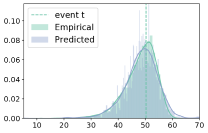
(a) $\delta=1$ (observed)

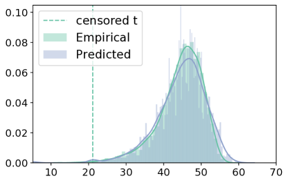
(b) $\delta=0$ (censored)

Figure 1. Two simulated time-to-event distributions with 30% event rate showing that VSI successfully predicts the underlying distributions from covariates. (left: events, right:censoring)

Prediction of subject-level distribution In practice, for each subject we only observe one $t$ from its underlying distribution. Our goal is to accurately predict the underlying distribution from the covariates $x$ alone (since $t$ and $\delta$ are not observed at test time), by learning from the observed instances. Figure 1 compares our VSI prediction with the ground-truth for two random subjects, which accurately recovers of individual survival distribution for both observed (Figure 1(a)) and censored cases (Figure 1(b)).

Table 1. KS statistic for simulation study.

Event Rate	100%	50%	30%
CoxPH (Oracle)	0.027	0.032	0.027
AFT-Weibull	0.057	0.058	0.068
MLP	0.047	0.063	0.064
VSI-NoQ	0.049	0.068	0.066
VSI	0.044	0.052	0.059

To systematically evaluate the consistency between the predicted and the true distributions, we compare average KS distance from models trained with various event rates in Table 1. Since the underlying generative process is based on CoxPH model, we consider the results from CoxPH as the oracle reference, since there is no model mis-specification. At 100% event rate (i.e., complete observation), apart from the oracle CoxPH, all models perform similarly. The VSI variants give slightly better results compared with MLP and AFT-Weibull. As the proportion of observed events decreases, VSI remains the best performing model, closely followed by the parametric AFT-Weibull. Note that neither MLP nor VSI-NoQ matches the performance of VSI, which suggests that the full VSI design better accommodates censoring observations.

Table 2. Model performance summary for simulation study based on $C_{td}$, C-Index and average test log-likelihood. Confidence Intervals for C-Index provided in the SM. For NA entries, the corresponding evaluation metric can not be applied.

Models	$C_{td}$			C-Index Raw			log-likelihood
	100%	50%	30%	100%	50%	30%	100%	50%	30%
CoxPH	0.757	0.755	0.761	0.773	0.781	0.793	NA	NA	NA
Coxnet	NA	NA	NA	0.776	0.784	0.760	NA	NA	NA
AFT-Weibull	0.742	0.750	0.768	0.773	0.781	0.793	-4.43	-2.29	-1.47
RSF	0.631	0.638	0.608	0.701	0.718	0.712	-14.12	-8.02	-5.35
DeepSurv	NA	NA	NA	0.772	0.781	0.793	NA	NA	NA
MLP	0.744	0.751	0.770	0.772	0.781	0.793	-4.15	-2.22	-1.41
VSI-NoQ	0.748	0.749	0.763	0.772	0.781	0.793	-4.16	-2.22	-1.41
VSI	0.748	0.756	0.772	0.773	0.781	0.793	-4.15	-2.22	-1.40

Average log-likelihood and C-Index To validate the effectiveness of VSI, we also provide a comprehensive summary of model performance against other popular or state-of-the-art alternatives in Table 2, under various simulation setups with different evaluation metrics. VSI consistently outperforms its counterparts in terms of the average log-likelihood and time-dependent C-Index. Together with the observation that VSI also yields better KS distance (see Table 1), converging evidence suggests our VSI better predicts the individual survival distributions relative to other competing solutions.

We also compared the raw C-Index and the corresponding confidence intervals using the weighted average of model predicted survival time (defined in Sec 3.5) as the risk score, and we did not find significant differences between alternative methods, as shown in Table 2 and Supplemental Materials. Thus VSI can deliver comparable performance relative to models that are compatible with the data generating mechanism. Raw C-Index quantifies the corresponding pairs without considering the time horizon, thus the distinctions among good performing models are not significant.

To provide a more informative summary, We plot the test log-likelihood distributions for selected models in Figure 2. We can see that VSI log-likelihoods estimates are tighter and higher for both observed and censored observations, especially when we have low event rates. The $(0.10,0.90)$ percentiles range for simulation studies please refer to SM.

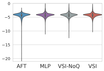
(a)

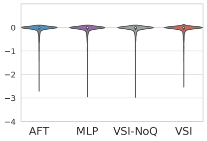
(b)

Figure 2. Test log-likelihood distributions for the 50% event rate simulation dataset. (left: events, right:censoring)

Coverage Plots In Figure 3, VSI achieves both relatively high coverage for event (Figure 3(a)) and censored observations (Figure 3(b)), comparing to the oracle method CoxPH in this synthetic example. Note that while RSF performs better for the observed events, its performance on censored cases falls well below other solutions.

We refer the readers to our Supplementary Materials for additional simulations and analyses based on toy models.

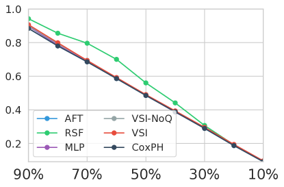
(a)

(b)

Figure 3. Test coverage rate for the 50% event rate simulation dataset. (left: events, right: censoring)

6.3. Real-World datasets

Moving beyond toy simulations, we further compare VSI to competing solution on the following three real-world datasets, $i$) FLCHAIN (Dispenzieri et al., 2012): a public dataset to determine whether the elevation in free light chain assay provides prognostic information to the general population survival, $ii$) SUPPORT (Knaus et al., 1995): a public dataset for a prospective cohort study to estimate survival over seriously ill hospitalized adults for 180 days period, and $iii$) SEER (Ries et al., 2007): a public dataset aim to study cancer survival among adults, which contains 1988 to 2001 information, provided by U.S. Surveillance, Epidemiology, and End Results (SEER) Program. In this experiments, we used 10-year follow-up breast cancer subcohort in SEER dataset. We follow the data pre-processing steps outlined in Chapfuwa et al. (2018). To handle the missing values in data, we adopt the common practice of median imputation for continuous variables and mode imputation for discrete variables.

Table 3. Summary Statistics for Real Datasets.

	FLCHAIN	SUPPORT	SEER
$N$	7,894	9,105	68,082
Event rate($\%$)	27.5	68.1	51.0
$p$(cat)	26(21)	59(31)	789(771)
NaN($\%$)	2.1	12.6	23.4
Max event $t$	$4998_{\text{days}}$	$1944_{\text{days}}$	$120_{\text{months}}$
Loss of Info($\%$)	10.45	1.57	0.0

Summary statistics of the datasets are shown in Table 3, where $N$ is the total number of observations, $p$ denotes the total number of variables after one-hot-encoding, NaN($\%$) stands for the proportion of missingness in covariates, and loss of information stands for the proportion of censoring observations happened after the maximum event time $t$.

Table 4. Summary for Real Datasets based on C-Index and average log-likelihood. Confidence Intervals for C-Index are provided in SM. NA implies the corresponding evaluation metric can not be evaluated.

Models	$C_{td}$			C-Index Raw			log-likelihood
	FLCHAIN	SUPPORT	SEER	FLCHAIN	SUPPORT	SEER	FLCHAIN	SUPPORT	SEER
Coxnet	NA	NA	NA	0.790	0.797	0.819	NA	NA	NA
AFT-Weibull	0.777	0.752	NA	0.792	0.797	NA	-3.09	-4.39	NA
RSF	NA	NA	NA	0.771	0.751	0.796	NA	NA	NA
DeepSurv	NA	NA	NA	0.785	0.678	NA	NA	NA	NA
MLP	0.775	0.768	0.821	0.751	0.811	0.811	-1.91	-2.86	-2.50
VSI-NoQ	0.745	0.772	0.820	0.745	0.824	0.809	-2.45	-2.79	-2.50
VSI	0.787	0.775	0.824	0.792	0.827	0.826	-1.85	-2.74	-2.49

Table 5. Quantile ranges for $\log$-likelihood in Real Datasets. Note AFT did not converge to reasonable solutions for SEER.

Models	Observed			Censored
	flchain	support	seer	flchain	support	seer
AFT	2.491	4.706	NA	0.468	1.850	NA
MLP	2.970	4.273	1.780	0.518	1.540	0.623
VSI-NoQ	7.34	4.744	1.801	0.559	1.634	0.529
VSI	2.213	4.143	1.718	0.537	1.354	0.508

In Table 4 we compare the C-Indices and average log-likelihood. The advantage of VSI is more evident for the more challenging real datasets, especially in the cases of low observed event rates. For example, with 30% event rate, in SUPPORT dataset, VSI Confidence Interval for raw C-Index as (0.809, 0.846), while the standard CoxNet is only (0.763,0.805) and AFT (0.782,813), i.e., the overlaps with that of VSI are very small. Similar results were observed for other datasets and baseline solutions. VSI shows remarkable robustness against data incompleteness in a real-world scenario, achieving the best results according to all three metrics. For VSI the raw C-Index is computed from the weighted average of VSI predicted distribution, please refer to SM for more details.

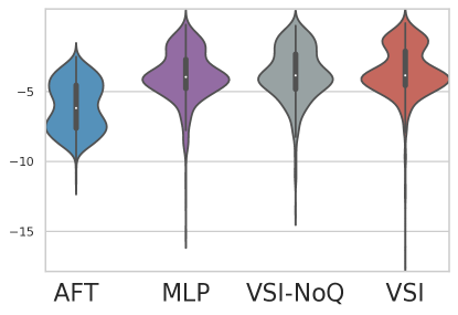
(a)

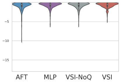
(b)

Figure 4. $\log$-likelihood distributions for SUPPORT Dataset, (left: events, right:censoring)

In Figure 4, the distribution of $\log$-likelihood is more concentrated, in addition to a higher mean. To quantitatively evaluate the concentration, we report the difference between $10\%$ and $90\%$ quantiles of $\log$-likelihood in Table 5. The quantile ranges of VSI are considerably smaller compared to alternative solutions under most experimental settings. This verifies VSI enjoys better model robustness compared to other popular alternatives, especially in the case of high censoring rates.

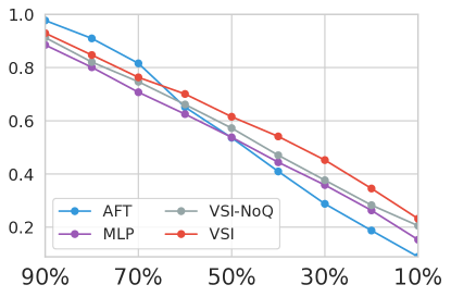
(a)

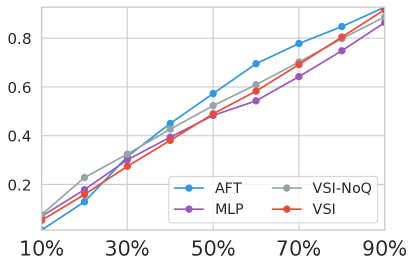
(b)

Figure 5. Coverage rate for SUPPORT Dataset, (left: events, right: censoring)

Together with the coverage plots in Figure 5, VSI has relative high coverage for both events and censoring cases which indicates better performance in capturing the true event time in challenging real-world datasets. The consistency of those results have been verified through repeated runs on these three datasets. For more detailed results please refer to SM.

7. CONCLUSIONS

We presented an approach for learning time-to-event distributions conditioned on covariates in a nonparametric fashion by leveraging a principled variational inference formulation. The proposed approach, VSI, extends the variational inference framework to survival data with censored observations. Based on synthetic and diverse real-world datasets, we demonstrated the ability of VSI to recover the underlying unobserved time-to-event distribution, as well as providing point estimations of time-to-event for subjects that yield excellent performance metrics consistently outperforming feed-forward deep learning models and traditional statistical models.

As future work, we plan to extend our VSI framework to longitudinal studies, where we can employ a recurrent neural net (RNN) to account for the temporal dependencies. For datasets with observations made at irregular intervals, for instance, the Neural-ODE model (Chen et al., 2018a) can be applied. Our work can be also adapted to make dynamic predictions of event times to serve the needs of modern clinical practices.

Acknowledgements

The authors would like to thank the anonymous reviewers for their insightful comments. This research was supported in part by by NIH/NIBIB R01-EB025020.

Appendix A Implementing VSI

For model inputs, we encode each subject’s time with a one-hot vector $t^{\text{OH}}$ with dimension $(1\times M)$ based on the observed event $t_{i}$ for subject $(\delta_{i}=1)$. With event $t$ has been one-hot-encoded, only one bin where the event time falls in equals 1, else equal 0. For censoring observations $(\delta_{i}=0)$ we have partial information about the true unknown event time, instead of missingness. We know for sure that the events would happen after the observed censored time $t_{i}$. The input vector, timepoints after the censored time $t_{i}$ have been put a prior based on population time-to-event distribution by Nelson-Aalen Estimator. This re-weighting strategy informs the model that this subject didn’t have event before time $t_{i}$, and also regularizes the model with respect to empirical tail distribution. One may also choose not to encode $t_{i}$ but adding $\delta_{i}$ to the input as well. In this case, each subject in the training has input of the form $(x_{i},t_{i},\delta_{i})$. To predict new $t$, the input for the prediction process is $(x_{i},\delta=1)$ where by defaut we are predicting the time-to-event. We have shown by experiments the two form of inputs produce similar results and the encoding strategy performs better under both simulation and real-world scenarios. The KS statistic for 30% event rates has 0.073, well VSI has 0.059.

Population Survival Estimation Based on Nelson-Aalen Estimator For NA estimator, $\tilde{H}(t)=\sum_{t_{j}\leq t}\frac{d_{j}}{n_{j}}$. Therefore we could calculate $f(t)$ accordingly. Let the selected discretized time be $t_{(b)}$, where $b\in\{1,\ldots,M\}$.

$$\begin{split}\tilde{H}(t_{(b)})&=\sum_{j\leq b}\frac{d_{j}}{n_{j}}\\ \tilde{S}(t_{(b)})&=\exp(-\tilde{H}(t_{(b)}))\\ \tilde{f}(t_{(1)})&=1-\tilde{S}(t_{(1)})\\ \tilde{f}(t_{(b)})&=\tilde{S}(t_{(b)})-\tilde{S}(t_{(b-1)})\\ &=\exp(-\sum_{j\leq b}\frac{d_{j}}{n_{j}})-\exp(-\sum_{j\leq b-1}\frac{d_{j}}{n_{j}})\\ \tilde{f}(t_{(M)})&=1-\sum_{b=1}^{M-1}\tilde{f}(t_{(b)})\end{split}$$

Therefore the we have $[\tilde{f}(t_{(1)}),\tilde{f}(t_{(2)}),\ldots,\tilde{f}(t_{(M)})]$ accordingly for each timepoint. For each censored subject where the censored time falls in bin $k$,

$$t^{\text{OH}}_{(b)}=\begin{cases}0,&\text{if }b\leq k\\ \frac{\tilde{f}(t_{(b)})}{\sum_{b>k}\tilde{f}(t_{(b)})},&\text{if }b>k\end{cases}$$

In this way the constructed $\sum_{b}t^{\text{OH}}_{(b)}=1$ as well. Now we have the soft one-hot-encoding for original censored $t$.

Architecture for VSI The input of VSI is $Y_{i}=(x_{i},\delta_{i},t^{\text{OH}}_{i})$. Parameters for $p_{\theta}(z|x)$ and $q_{\phi}(z|t^{\text{OH}}_{i},x)$ were obtained by two MLP framework respectively, each with hidden dimensions $[32,32]$ with output dimension $[32]$. The decoding arm $p_{\theta}(t_{i}|z)$ has hidden dimensions $[32,32,32]$ with output a $(1\times M)$ vector which is the predicted logits. Activation function is leaky ReLU, continuous variables are z-transformed before entering the model based on training datasets.

Appendix B Derivation of Likelihood lowerbound for censored observations

To get the likelihood lowerbound for censored observations, we applied Fubini’s theorem and Jensen’s inequality.

$$\begin{split}&\mathcal{L}_{c}(x_{i},t_{i};\theta)\\ &=\text{log }S_{\theta}(t_{i}|x_{i})\\ &=\text{log }\int_{t_{i}}^{\infty}p_{\theta}(t|x_{i})dt\\ &=\text{log }\int_{t_{i}}^{\infty}\int_{z}p_{\theta}(t,z|x_{i})dzdt\\ &=\text{log }\int_{t_{i}}^{\infty}\int_{z}\frac{p_{\theta}(z,t|x_{i})}{q_{\phi}(z|t_{i},x_{i})}q_{\phi}(z|t_{i},x_{i})dzdt\\ &=\text{log }\int_{t_{i}}^{\infty}\int_{q_{\phi}(z|t_{i},x_{i})}\frac{p_{\theta}(z,t|x_{i})}{q_{\phi}(z|t_{i},x_{i})}dQ(z|t_{i},x_{i})dt\\ &=\text{log }\int_{q_{\phi}(z|t_{i},x_{i})}\int_{t_{i}}^{\infty}\frac{p_{\theta}(z,t|x_{i})}{q_{\phi}(z|t_{i},x_{i})}dtdQ(z|t_{i},x_{i})\\ &=\text{log }\int_{q_{\phi}(z|t_{i},x_{i})}\int_{t_{i}}^{\infty}p_{\theta}(t|z)\frac{p_{\theta}(z|x_{i})}{q_{\phi}(z|t_{i},x_{i})}dtdQ(z|t_{i},x_{i})\\ &=\text{log }\int_{q_{\phi}(z|t_{i},x_{i})}\frac{p_{\theta}(z|x_{i})}{q_{\phi}(z|t_{i},x_{i})}\int_{t_{i}}^{\infty}p_{\theta}(t|z)dtdQ(z|t_{i},x_{i})\\ &\geq\int_{q_{\phi}(z|t_{i},x_{i})}\text{log }\left(\frac{p_{\theta}(z|x_{i})}{q_{\phi}(z|t_{i},x_{i})}\int_{t_{i}}^{\infty}p_{\theta}(t|z)dt\right)dQ(z|t_{i},x_{i})\\ &=\mathbb{E}_{q_{\phi}(z|t,x)}[\text{log }{\frac{p_{\theta}(z|x_{i})}{q_{\phi}(z|t_{i},x_{i})}}+\text{log }S_{\theta}(z,t_{i}|x_{i})]\\ &=L_{c}(x_{i},t_{i};\theta,\phi)\end{split}$$

Likelihood for Multivariate Normal Distribution The Multivariate Normal Log-likelihood function used for ELBO has $z_{l}\sim N(\mu,\Sigma)$ , where $z_{l}$ is $m\times 1$, $\mu$ is $m\times 1$ and $\Sigma$ is $m\times m$ :

$$\text{log }\mathcal{L}(z_{l};\mu,\Sigma)=-\frac{1}{2}[\text{log }(|\Sigma|)+(z_{l}-\mu)^{T}\Sigma^{-1}(z_{l}-\mu)+m\text{log }(2\pi)]$$

Appendix C Likelihood Calculation for Statistical Models

AFT Models Distributions of $T_{i}$ and $\epsilon_{i}$ are corresponding to each other, with:

(9) $$\begin{split}S_{i}(t|x_{i})&=S_{\epsilon_{i}}(z_{i})=S_{0}(\exp(\beta^{T}x_{i})t)\\ z_{i}&=\frac{log(t)-\mu-\theta^{T}x_{i}}{\sigma}\\ h_{i}(t|x_{i})&=\frac{1}{\sigma t_{i}}h_{\epsilon_{i}}(z_{i})=h_{0}(\exp(\beta^{T}x_{i})t)\end{split}$$

The likelihood function under general non-informative censoring has the form:

(10) $$\begin{split}\mathcal{L}(\mathcal{D};\theta)&=\prod_{i=1}^{n}h(t_{i}|x_{i})^{\delta_{i}}S(t_{i}|x_{i})\\ &=\prod_{i=1}^{n}(\sigma t_{i})^{-\delta_{i}}\{h_{\epsilon_{i}}(z_{i})\}^{\delta_{i}}S_{\epsilon_{i}}(z_{i})\end{split}$$

For AFT model with Weibull distribution, $\epsilon_{i}$ follows the extreme value distribution and $T_{i}$ follows the Weibull distribution, with scale parameter $\lambda>0$, shape parameter $\nu>0$.

$$\begin{split}f_{0}(t)&=\lambda\nu t^{\nu-1}\exp(-\lambda t^{\nu})\\ h_{0}(t)&=\lambda\nu t^{\nu-1}\\ S_{0}(t)&=\exp(-\lambda t^{\nu})\\ \mathbb{E}(T)&=\frac{1}{\lambda^{1/\nu}}\Gamma(\frac{1}{\nu}+1)\\ S_{\epsilon}(z)&=\exp(-\exp(z))\\ f_{\epsilon}(z)&=\exp(z)\exp(-\exp(z))\\ h_{\epsilon}(z)&=\frac{f_{\epsilon}(z)}{S_{\epsilon}(z)}\\ &=\exp(z)\end{split}$$

Thus $\lambda=\exp(-\mu/\sigma)$ and $\nu=1/\sigma$ in the extreme value distribution $\epsilon$, equivalently $\mu=-\frac{\log\lambda}{\nu}$ and $\sigma=1/\nu$. Thus the log-likelihood is:

(11) $$\begin{split}&\log\mathcal{L}_{\text{Weibull}}(\mathcal{D};\theta)\\ &=\sum_{i=1}^{n}\left[-\delta_{i}\log(\sigma t_{i})+\delta_{i}\log\{h_{\epsilon_{i}}(z_{i})\}+\log S_{\epsilon_{i}}(z_{i})\right]\\ &=\sum_{i=1}^{n}\left[\delta_{i}\log(\nu)-\delta_{i}\log(t_{i})+\delta_{i}z_{i}-\exp(z_{i})\right]\end{split}$$

Note that for comparison log-likelihood at same scale, AFT and other parametric methods’ log-likelihood were calculated at discretized event time same as VSI.

Random Survival Forest

Random Survival Forest could give estimates for cumulative hazard function at the pre-specifed timepoints $\hat{H}(t_{(b)}),b\in\{1,ldots,M\}$, which could let us get the estimated survival function and time-to-event distribution.

$$\begin{split}\hat{S}(t_{(b)})&=\exp(-\hat{H}(t_{(b)}))\\ \hat{f}(t_{(1)})&=1-\hat{S}(t_{(1)})\\ \hat{f}(t_{(b)})&=\hat{S}(t_{(b)})-\hat{S}(t_{(b-1)})\\ \hat{f}(t_{(M)})&=1-\sum_{b=1}^{M-1}\hat{f}(t_{(b)})\\ \end{split}$$

Then based on the survival likelihood function

$$\mathcal{L}(\mathcal{D};\theta)=\prod_{i=1}^{n}\hat{p}(t_{i}|x_{i})^{\delta_{i}}\hat{S}(t_{i}|x_{i})^{1-\delta_{i}}$$

, we could get the likelihood for RSF.

Cox Models

Since cox model is semiparametric, we don’t know the full parameters, therefore usually we would give partial likelihood instead of full likelihood.

$$\begin{split}PL(\beta)=\prod_{i=1}^{n}\{\frac{\exp(\beta^{T}x_{i})}{\sum_{l\in R(t_{(i)})}\exp(\beta^{T}x_{i})}\}\end{split}$$

$R(t_{(i)})$ is the set of subjects at risk at time $t_{(i)}$. Above partial likelihood is from multiply the probability that a subject with covariates $x_{i}$ dies in $(t_{(i)},t_{(i)}+\delta t]$ with $\delta t\rightarrow 0$ for each subject with event. $\hat{\beta}$ is obtained by Maximize $\log PL(\beta)$.

To make comparison between difference method, we would use some empirical way to calculate the full likelihood for Cox models.

$$\begin{split}\mathcal{L}(\mathcal{D};\theta)&=\prod_{i=1}^{n}h(t_{i}|x_{i})^{\delta_{i}}S(t_{i}|x_{i})\\ \log\mathcal{L}(\mathcal{D};\theta)&=\sum_{i=1}^{n}\delta_{i}[\log h_{0}(t_{i})+\beta^{T}x_{i}]+\log S(t_{i}|x_{i})\end{split}$$

In above equations, we would use the estimated $h_{0}(t)$ and predicted $S(t_{i}|x_{i})$.

Appendix D Additional Results for Simulation Datasets

Distribution of log-likelihood The distributions of log-likelihoods for simulation datasets are shown in Figure S1. In all scenarios, VSI has the most concentrated distribution of the log-likelihood, which suggests that VSI is robust under different event rate with CoxPH assumptions. MLP and VSI-NoQ performed equally good in this simple synthetic study.

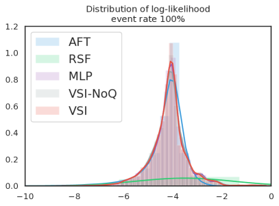
(a)

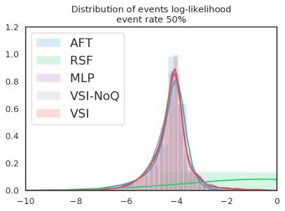
(b)

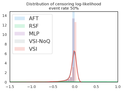
(c)

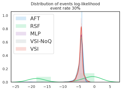
(d)

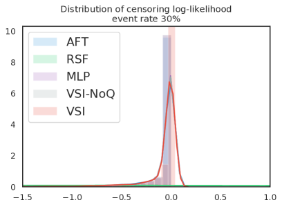
(e)

Figure S1. Testing datasets log-likelihood distributions for simulation dataset. $100\%$ event rate (a), $50\%$ event rate (observed:b, censored:c), $30\%$ event rate (observed:d, censored:e)

The percentile ranges of $\log$-likelihood in simulation studies are shown in Table S1. When we have low event rates, VSI stands out from the baseline methods.

Table S1. Quantile range [0.10, 0.90] of $\log$-likelihood in Simulation Study

Models	Observed			Censored
	100%	50%	30%	50%	30%
AFT-Weibull	1.55	1.67	1.87	0.26	0.28
MLP	1.66	1.62	1.98	0.24	0.23
VSI-NoQ	1.70	1.59	1.99	0.25	0.23
VSI	1.67	1.60	1.68	0.23	0.27

Confidence Intervals for Raw C-Index To better capture the differences in raw C-Index, the confidence intervals for each simulation strategy are calculated (See Table S2). We have comparable performance with oracle methods with regarding to this metric. More illustrative metrics have been discussed in the text.

Table S2. Raw C-Index with confidence intervals (in parentheses) for simulation studies. RSF and DeepSurv do not provide intrinsic methods to calculate confidence intervals

Event Rate	100%	50%	30%
CoxPH	0.773 (0.768, 0.777)	0.781 (0.775, 0.788)	0.793 (0.785, 0.802)
Coxnet	0.776 (0.762, 0.789)	0.784 (0.763, 0.805)	0.760 (0.730, 0.791)
AFT-Weibull	0.773 (0.768, 0.777)	0.781 (0.775, 0.788)	0.793 (0.785, 0.802)
RSF	0.701	0.718	0.712
DeepSurv	0.772	0.781	0.793
MLP	0.772 (0.767, 0.777)	0.781 (0.775, 0.788)	0.793 (0.784, 0.801)
VSI-NoQ	0.772 (0.768, 0.777)	0.781 (0.774, 0.788)	0.793 (0.784, 0.801)
VSI	0.773 (0.768, 0.777)	0.781 (0.775, 0.788)	0.793 (0.784, 0.801)

Coverage Rate To visualize the proportion of observed time is covered in the predicted personalized time-to-event distributions, we calculated the coverage rate for each percentile ranges. Our model balanced between events and censoring coverage the best among all methods. We compared the coverage with CoxPH, AFT-Weibull, VSI-NoQ, MLP and RSF. CoxPH could serves as the reference, since the simulation study is based on CoxPH assumptions entirely. The results are shown in Figure S2.

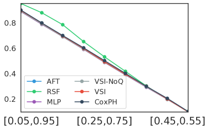
(a)

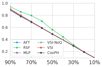
(b)

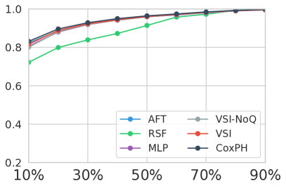
(c)

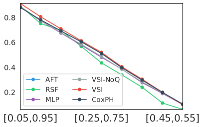
(d)

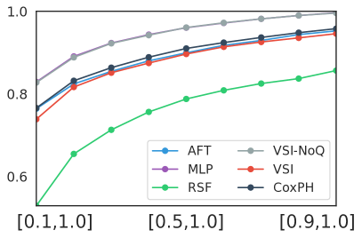
(e)

Figure S2. Testing datasets Coverage rate for simulation datasets. $100\%$ event rate (a), $50\%$ event rate (observed:b, censored:c), $30\%$ event rate (observed:d, censored:e)

Appendix E Additional Results for Real Datasets

Comparison of Weighted Average and Median In Table S3, we compared the C-Index calculated with weighted average and median for real datasets, with weighted average higher in general. In simulation studies, those two numbers are similar to each other.

Table S3. Comparison median and weighted average for predicted time-to-event distribution with C-index in real datasets

C-Index	FLCHAIN	SUPPORT	SEER
Median	0.774	0.833	0.814
Weighted Average	0.792	0.823	0.826

Distribution for Log-likelihood Log-likelihood distribution for real datasets shown in Figure S3. Similar to the case discussed in the text, VSI performs consistently better in all three realworld datasets.

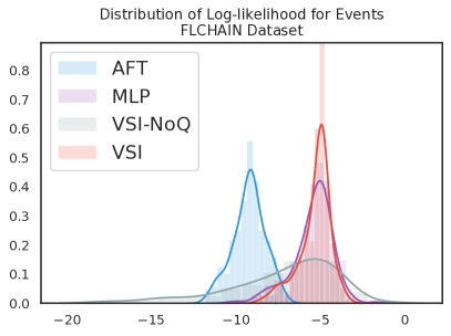
(a)

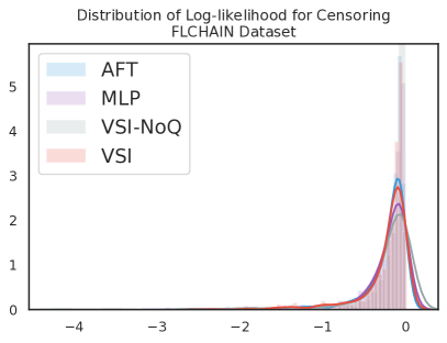
(b)

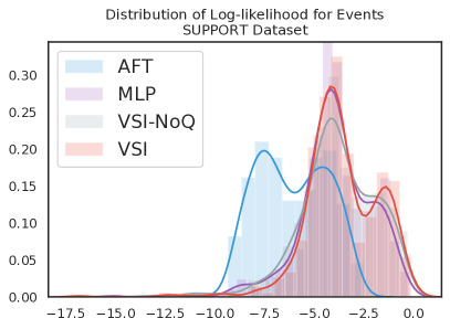
(c)

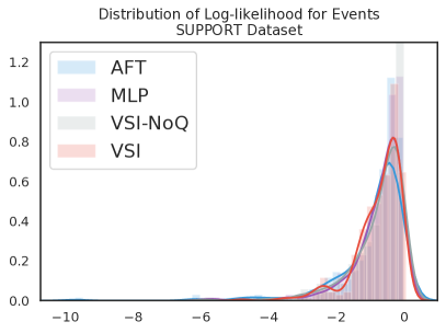
(d)

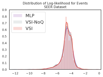
(e)

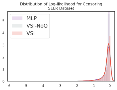
(f)

Figure S3. Likelihood distributions for real datasets. FLCHAIN (observed: a, censored: b), SUPPORT (observed: c, censored: d), SEER (observed: e, censored: f)

Confidence Intervals for Raw C-Index As shown in Table S4, raw C-Index for VSI is significantly better than other method with relatively tight confidence intervals.

Table S4. Raw C-Index with confidence intervals (in parentheses) for Real Data. NA indicates the corresponding evaluation metric cannot be evaluated. RSF and DeepSurv do not provide intrinsic methods to calculate confidence intervals.

Event Rate	FLCHAIN	SUPPORT	SEER
Coxnet	0.790 (0.761, 0.820)	0.784 (0.763, 0.805)	0.819 (0.812, 0.826)
AFT-Weibull	0.792 (0.763, 0.821)	0.797 (0.782, 0.813)	NA
RSF	0.771	0.751	0.796
DeepSurv	0.785	0.678	NA
MLP	0.751 (0.722, 0.781)	0.811 (0.791, 0.831)	0.811 (0.803, 0.818)
VSI-NoQ	0.745 (0.714, 0.777)	0.824 (0.804, 0.843)	0.809 (0.802, 0.817)
VSI	0.792 (0.762, 0.821)	0.827 (0.809, 0.846)	0.826 (0.819, 0.833)

Coverage rate for real datasets Cover rate for real datasets shown in Figure S4. VSI has relative high coverage for both events and censoring in all three datasets, which similar to the case we have in simulation datasets.

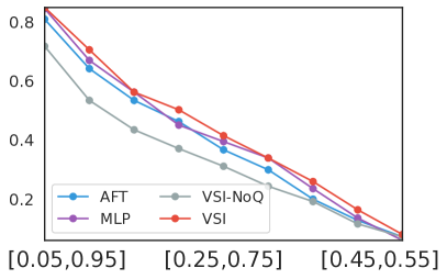
(a)

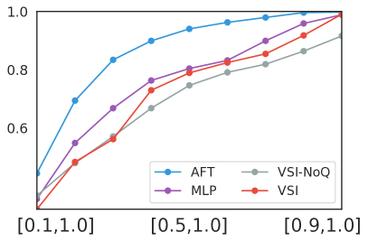
(b)

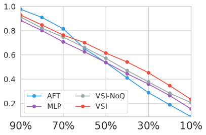
(c)

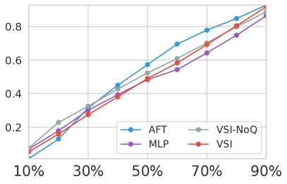
(d)

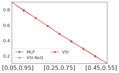
(e)

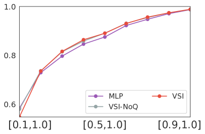
(f)

Figure S4. Coverage rates for real datasets. FLCHAIN (observed: a, censored: b), SUPPORT (observed: c, censored: d), SEER (observed: e, censored: f)

For the comparison models, VSI, MLP and VSI-NoQ and AFT-Weibull are distribution based and could give all statistics in the simulation studies. For RSF and CoxPH, which could calculate the estimated cumulative hazards, the corresponding survival function and time-to-event could be calculated accordingly. For DeepSurv and Coxnet, only raw C-Index can be given.

References

- (1)
- Aalen et al. (2008) Odd Aalen, Ornulf Borgan, and Hakon Gjessing. 2008. Survival and event history analysis: a process point of view. Springer Science & Business Media.
- Aalen (1994) Odd O Aalen. 1994. Effects of frailty in survival analysis. Statistical Methods in Medical Research 3, 3 (1994), 227–243.
- Alaa and van der Schaar (2017) Ahmed M Alaa and Mihaela van der Schaar. 2017. Deep multi-task gaussian processes for survival analysis with competing risks. In Proceedings of the 31st International Conference on Neural Information Processing Systems. Curran Associates Inc., 2326–2334.
- Antolini et al. (2005) Laura Antolini, Patrizia Boracchi, and Elia Biganzoli. 2005. A time-dependent discrimination index for survival data. Statistics in Medicine 24, 24 (2005), 3927–3944.
- Bender et al. (2005) Ralf Bender, Thomas Augustin, and Maria Blettner. 2005. Generating survival times to simulate Cox proportional hazards models. Statistics in medicine 24, 11 (2005), 1713–1723.
- Bou-Hamad et al. (2011) Imad Bou-Hamad, Denis Larocque, Hatem Ben-Ameur, et al. 2011. A review of survival trees. Statistics Surveys 5 (2011), 44–71.
- Burda et al. (2015) Yuri Burda, Roger Grosse, and Ruslan Salakhutdinov. 2015. Importance weighted autoencoders. arXiv preprint arXiv:1509.00519 (2015).
- Chapfuwa et al. (2018) Paidamoyo Chapfuwa, Chenyang Tao, Chunyuan Li, Courtney Page, Benjamin Goldstein, Lawrence Carin, and Ricardo Henao. 2018. Adversarial time-to-event modeling. arXiv preprint arXiv:1804.03184 (2018).
- Chen et al. (2018b) Liqun Chen, Chenyang Tao, Ruiyi Zhang, Ricardo Henao, and Lawrence Carin Duke. 2018b. Variational inference and model selection with generalized evidence bounds. In International Conference on Machine Learning. 892–901.
- Chen et al. (2018a) Tian Qi Chen, Yulia Rubanova, Jesse Bettencourt, and David K Duvenaud. 2018a. Neural ordinary differential equations. In Advances in neural information processing systems. 6571–6583.
- Cox (1972) David R Cox. 1972. Regression models and life-tables. Journal of the Royal Statistical Society: Series B (Methodological) 34, 2 (1972), 187–202.
- Dispenzieri et al. (2012) Angela Dispenzieri, Jerry A Katzmann, Robert A Kyle, Dirk R Larson, Terry M Therneau, Colin L Colby, Raynell J Clark, Graham P Mead, Shaji Kumar, L Joseph Melton III, et al. 2012. Use of nonclonal serum immunoglobulin free light chains to predict overall survival in the general population. In Mayo Clinic Proceedings, Vol. 87. Elsevier, 517–523.
- Faraggi and Simon (1995) David Faraggi and Richard Simon. 1995. A neural network model for survival data. Statistics in medicine 14, 1 (1995), 73–82.
- Fard et al. (2016) Mahtab Jahanbani Fard, Ping Wang, Sanjay Chawla, and Chandan K Reddy. 2016. A bayesian perspective on early stage event prediction in longitudinal data. IEEE Transactions on Knowledge and Data Engineering 28, 12 (2016), 3126–3139.
- Fernández et al. (2016) Tamara Fernández, Nicolás Rivera, and Yee Whye Teh. 2016. Gaussian processes for survival analysis. In Advances in Neural Information Processing Systems. 5021–5029.
- Fotso (2018) Stephane Fotso. 2018. Deep Neural Networks for Survival Analysis Based on a Multi-Task Framework. arXiv preprint arXiv:1801.05512 (2018).
- Harrell et al. (1982) Frank E Harrell, Robert M Califf, David B Pryor, Kerry L Lee, and Robert A Rosati. 1982. Evaluating the yield of medical tests. Jama 247, 18 (1982), 2543–2546.
- Hougaard (1995) Philip Hougaard. 1995. Frailty models for survival data. Lifetime data analysis 1, 3 (1995), 255–273.
- Ishwaran et al. (2008) Hemant Ishwaran, Udaya B Kogalur, Eugene H Blackstone, Michael S Lauer, et al. 2008. Random survival forests. The annals of applied statistics 2, 3 (2008), 841–860.
- Kalbfleisch and Prentice (2011) John D Kalbfleisch and Ross L Prentice. 2011. The statistical analysis of failure time data. Vol. 360. John Wiley & Sons.
- Kaplan and Meier (1958) Edward L Kaplan and Paul Meier. 1958. Nonparametric estimation from incomplete observations. Journal of the American statistical association 53, 282 (1958), 457–481.
- Katzman et al. (2016) Jared L Katzman, Uri Shaham, Alexander Cloninger, Jonathan Bates, Tingting Jiang, and Yuval Kluger. 2016. Deep survival: A deep cox proportional hazards network. stat 1050 (2016), 2.
- Katzman et al. (2018) Jared L Katzman, Uri Shaham, Alexander Cloninger, Jonathan Bates, Tingting Jiang, and Yuval Kluger. 2018. DeepSurv: personalized treatment recommender system using a Cox proportional hazards deep neural network. BMC medical research methodology 18, 1 (2018), 24.
- Khan and Zubek (2008) Faisal M Khan and Valentina Bayer Zubek. 2008. Support vector regression for censored data (SVRc): a novel tool for survival analysis. In 2008 Eighth IEEE International Conference on Data Mining. IEEE, 863–868.
- Kingma and Welling (2013) Diederik P Kingma and Max Welling. 2013. Auto-encoding variational bayes. arXiv preprint arXiv:1312.6114 (2013).
- Knaus et al. (1995) William A Knaus, Frank E Harrell, Joanne Lynn, Lee Goldman, Russell S Phillips, Alfred F Connors, Neal V Dawson, William J Fulkerson, Robert M Califf, Norman Desbiens, et al. 1995. The SUPPORT prognostic model: objective estimates of survival for seriously ill hospitalized adults. Annals of internal medicine 122, 3 (1995), 191–203.
- Li et al. (2019) Hongming Li, Pamela Boimel, James Janopaul-Naylor, Haoyu Zhong, Ying Xiao, Edgar Ben-Josef, and Yong Fan. 2019. Deep Convolutional Neural Networks for Imaging Data Based Survival Analysis of Rectal Cancer. arXiv preprint arXiv:1901.01449 (2019).
- Lisboa et al. (2003) Paulo JG Lisboa, H Wong, P Harris, and Ric Swindell. 2003. A Bayesian neural network approach for modelling censored data with an application to prognosis after surgery for breast cancer. Artificial intelligence in medicine 28, 1 (2003), 1–25.
- Luck et al. (2017) Margaux Luck, Tristan Sylvain, Héloïse Cardinal, Andrea Lodi, and Yoshua Bengio. 2017. Deep learning for patient-specific kidney graft survival analysis. arXiv preprint arXiv:1705.10245 (2017).
- Massey Jr (1951) Frank J Massey Jr. 1951. The Kolmogorov-Smirnov test for goodness of fit. Journal of the American statistical Association 46, 253 (1951), 68–78.
- Murphy et al. (1997) SA Murphy, AJ Rossini, and Aad W van der Vaart. 1997. Maximum likelihood estimation in the proportional odds model. J. Amer. Statist. Assoc. 92, 439 (1997), 968–976.
- Neal (2001) Radford M Neal. 2001. Annealed importance sampling. Statistics and computing 11, 2 (2001), 125–139.
- Raftery (1995) Adrian E Raftery. 1995. Bayesian model selection in social research. Sociological methodology 25 (1995), 111–164.
- Raftery et al. (1996) Adrian E Raftery, David Madigan, and Chris T Volinsky. 1996. Accounting for model uncertainty in survival analysis improves predictive performance. Bayesian statistics 5 (1996), 323–349.
- Rainforth et al. (2018) Tom Rainforth, Adam R Kosiorek, Tuan Anh Le, Chris J Maddison, Maximilian Igl, Frank Wood, and Yee Whye Teh. 2018. Tighter variational bounds are not necessarily better. arXiv preprint arXiv:1802.04537 (2018).
- Ranganath et al. (2014) Rajesh Ranganath, Sean Gerrish, and David Blei. 2014. Black box variational inference. In Artificial Intelligence and Statistics. 814–822.
- Ranganath et al. (2016) Rajesh Ranganath, Adler Perotte, Noémie Elhadad, and David Blei. 2016. Deep survival analysis. arXiv preprint arXiv:1608.02158 (2016).
- Resnick (2003) Sidney Resnick. 2003. A probability path. Birkhauser Verlag AG.
- Ries et al. (2007) LA Gloeckler Ries, JL Young, GE Keel, MP Eisner, YD Lin, MJ Horner, et al. 2007. SEER survival monograph: cancer survival among adults: US SEER program, 1988-2001, patient and tumor characteristics. National Cancer Institute, SEER Program, NIH Pub 07-6215 (2007), 193–202.
- Schwarzer et al. (2000) Guido Schwarzer, Werner Vach, and Martin Schumacher. 2000. On the misuses of artificial neural networks for prognostic and diagnostic classification in oncology. Statistics in medicine 19, 4 (2000), 541–561.
- Simon et al. (2011) Noah Simon, Jerome Friedman, Trevor Hastie, and Rob Tibshirani. 2011. Regularization paths for Cox’s proportional hazards model via coordinate descent. Journal of statistical software 39, 5 (2011), 1.
- Srivastava et al. (2014) Nitish Srivastava, Geoffrey Hinton, Alex Krizhevsky, Ilya Sutskever, and Ruslan Salakhutdinov. 2014. Dropout: a simple way to prevent neural networks from overfitting. The journal of machine learning research 15, 1 (2014), 1929–1958.
- Tomczak and Welling (2017) Jakub M Tomczak and Max Welling. 2017. VAE with a VampPrior. arXiv preprint arXiv:1705.07120 (2017).
- Wainwright and Jordan (2008) Martin J. Wainwright and Michael I. Jordan. 2008. Graphical Models, Exponential Families, and Variational Inference. Foundations and Trends in Machine Learning 1 (2008), 1–305.
- Wang et al. (2019) Ping Wang, Yan Li, and Chandan K Reddy. 2019. Machine learning for survival analysis: A survey. ACM Computing Surveys (CSUR) 51, 6 (2019), 110.
- Yu et al. (2011) Chun-Nam Yu, Russell Greiner, Hsiu-Chin Lin, and Vickie Baracos. 2011. Learning patient-specific cancer survival distributions as a sequence of dependent regressors. In Advances in Neural Information Processing Systems. 1845–1853.
- Zhang and Lu (2007) Hao Helen Zhang and Wenbin Lu. 2007. Adaptive Lasso for Cox’s proportional hazards model. Biometrika 94, 3 (2007), 691–703.
- Zhang and Zhou (2018) Quan Zhang and Mingyuan Zhou. 2018. Nonparametric Bayesian Lomax delegate racing for survival analysis with competing risks. In Advances in Neural Information Processing Systems. 5002–5013.
- Zupan et al. (1999) Blaž Zupan, Janez Demšar, Michael W Kattan, J Robert Beck, and Ivan Bratko. 1999. Machine learning for survival analysis: a case study on recurrence of prostate cancer. In Joint European Conference on Artificial Intelligence in Medicine and Medical Decision Making. Springer, 346–355.