Monte Carlo study of the tip region of branching random walks evolved to large times

Abstract

We implement a discretization of the one-dimensional branching Brownian motion in the form of a Monte Carlo event generator, designed to efficiently produce ensembles of realizations in which the rightmost lead particle at the final time $T$ is constrained to have a position $X$ larger than some predefined value $X_{\text{min}}$. The latter may be chosen arbitrarily far from the expectation value of $X$, and the evolution time after which observables on the particle density near the lead particle are measured may be as large as $T\sim 10^{4}$. We then calculate numerically the probability distribution $p_{n}(\Delta x)$ of the number $n$ of particles in the interval $[X-\Delta x,X]$ as a function of $\Delta x$. When ${X_{\text{min}}}$ is significantly smaller than the expectation value of the position of the rightmost lead particle, i.e. when $X$ is effectively unconstrained, we check that both the mean and the typical values of $n$ grow exponentially with $\Delta x$, up to a linear prefactor and to finite-$T$ corrections. When $X_{\text{min}}$ is picked far ahead of the latter but within a region extending over a size of order $\sqrt{T}$ to its right, the mean value of the particle number still grows exponentially with $\Delta x$, but its typical value is lower by a multiplicative factor consistent with $e^{-\zeta\Delta x^{2/3}}$, where $\zeta$ is a number of order unity. These numerical results bring strong support to recent analytical calculations and conjectures in the infinite-time limit.

1 Introduction

Understanding correlations of particles generated by one-dimensional branching random walks is an outstanding general problem in mathematics, with numerous potential applications in different fields of science. Various observables sensitive to these correlations may be derived from solutions to the Fisher-Kolmogorov-Petrovsky-Piscounov (FKPP) equation [1, 2] when the underlying stochastic process is the branching Brownian motion, or to an equation in the same universality class when the underlying process is some branching random walk.

The FKPP equation is relevant to many contexts (for a review, see e.g. [3]). In biology, it may describe the spread of a gene or of a disease in a population: This is the field in which it was first written down in the literature [1, 2]. In chemistry, it stems from a mean-field approximation for reaction-diffusion processes. In computer science, it appears in the study of the statistics of the heights of search trees [4]. In physics, it was also shown to be relevant for quite unexpected problems: For example, to understand the mean-field theory of disordered systems such as spin glasses or directed polymers in random media [5], and to describe some properties of scattering processes in elementary particle physics (for a review, see e.g. [6]). The latter was the initial motivation of the particle physicists for studying the FKPP equation [7].

Of particular interest here is the fact that the FKPP equation (or, more generally, FKPP-like equations) encodes the time evolution of generating functions of particle number probabilities $p_{n}(\Delta x)$ in intervals spanning a fixed distance $\Delta x$ to the left of the position $X$ of the rightmost particle in realizations of the branching Brownian motion (or, more generally, of branching random walks) [8]. So the problem of understanding these distributions of particles may be formulated elegantly in terms of equations in the universality class of the FKPP equation. Therefore, it essentially boils down to the well-defined mathematical problem of solving nonlinear partial differential equations. But since FKPP-like equations do not have complete analytical solutions, finding expressions for the observables of interest is not an easy task. On the other hand, these equations can be integrated numerically quite easily. However, extracting from these data either the probabilities $p_{n}(\Delta x)$ or their moments is in general not doable in practice, except for small values of $n$ and low-lying moments.

Recently, an analytical study of the generating function of $p_{n}(\Delta x)$ in the asymptotic limit of large $T$, large interval size $\Delta x$, and large distance $X-m_{T}$ between the position $X$ of the tip and its expectation value $m_{T}$ led to a few new results: The generating function was shown to exhibit a peculiar scaling form, and a conjecture for the typical value of $n$ as a function of $\Delta x$ was formulated [9]. While the scaling of the generating function could be checked by numerical integration of the relevant FKPP equation, arriving at a numerical determination of $p_{n}(\Delta x)$ requires a Monte Carlo implementation of the stochastic process. However, this is not straightforward, since the configurations of interest are very rare realizations of branching random walks evolved to large times. A naive implementation is doomed to fail. Algorithms to generate ensembles of rare events have been proposed in other contexts, see e.g. [10]. They would not directly apply to the problem we are addressing here, but as will be shown below, it is possible to design one specifically.

The main thrust of the present work is to introduce an algorithm for generating these rare realizations, and to apply an implementation of it to the numerical study of $p_{n}(\Delta x)$ as a function of the size of the interval $\Delta x$. The numerical output is eventually confronted to the analytical expectations.

The principle of the algorithm is explained in Sec. 2 in the case of the branching Brownian motion, and then of a branching random walk discrete in space and time, which is the process we implement numerically. The numerical results are presented in the subsequent Sec. 3, after a quick study of the model we have actually implemented and after a short review of the known analytical results and of the conjectures to be tested.

2 Generating realizations conditioned to a minimum position of the rightmost lead particle

For the sake of exposing the principle of the algorithm as simply as possible, we are first going to address the branching Brownian motion (BBM) process in one dimension. We shall then introduce a model of a branching random walk discrete in space and time, which is a discretization of the latter, that proves more convenient to implement in the form of a computer code.

2.1 Branching Brownian motion

The BBM of a set of particles is defined by two elementary processes: Each particle evolves in time independently of all the other particles through a Brownian motion in space, until it reaches the final time $T$, or until it is randomly replaced by two particles at its current position. For definiteness, we shall fix the diffusion constant to $\frac{1}{2}$, and the branching rate to unity. After a branching has occured, the offspring evolve further independently through the two same elementary processes (namely diffusion and branching).

A Monte Carlo implementation of the BBM is in principle straightforward, but since the number of particles in the system grows on the average exponentially with time, it is difficult to generate ensembles of realizations for times larger than typically $T\sim 10$: Indeed, with a continuous process, each particle must be followed individually. Furthermore, for our purpose which is to focus on rare events in which the lead particle is very far from its expected position, a naive implementation of the elementary processes is unpractical.

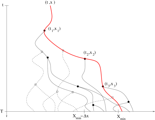
Specifically, we want to generate ensembles of realizations of the BBM which, at a (large) time $T$, contain at least one particle located at a position $X$ not smaller than some fixed ${X_{\text{min}}}$. The main idea of the algorithm is to mark the first particle from the beginning of the evolution, distinguishing it by conditioning its trajectory to arriving at a position in the interval $[{X_{\text{min}}},+\infty[$ at time $T$. This is illustrated in Fig. 1. A similar idea was proposed in Ref. [11], but it was not used for the purpose of numerical calculations.

2.1.1 Probability distribution of the first branching of the marked particle

We start with a single particle at time $t$, which we put at position $x$. We will need the probability $Q$ that there is no particle at or to the right of the position $x+\xi$ at time $t+\tau$ ($\xi$ may be any real number, $\tau$ is nonnegative) in the set generated by the BBM. It is well-known that it solves the FKPP equation

$$\partial_{\tau}Q(\tau,\xi)=\frac{1}{2}\partial_{\xi}^{2}Q(\tau,\xi)-Q(\tau,\xi)+Q^{2}(\tau,\xi)$$ (1)

with, as an initial condition, $Q(\tau=0,\xi)=1-\Theta(-\xi)$.

We now write down the probability density that the first splitting occurs at time $t_{1}\geq t$ at position $x_{1}$ and that there is at least one particle with position $x_{T}\geq{X_{\text{min}}}$ in the ensemble at time $T$. This probability density writes as the sum of two terms:

$$\pi_{T-t,{X_{\text{min}}}-x}(t_{1}-t,x_{1}-x)=\Theta(T-t_{1})\times e^{t-t_{1}}g(t_{1}-t,x_{1}-x)\left[1-Q^{2}(T-t_{1},{X_{\text{min}}}-x_{1})\right]\\ +\left[1-\Theta(T-t_{1})\right]\times e^{t-t_{1}}\int_{{X_{\text{min}}}}^{\infty}d\tilde{x}_{T}\,g(T-t,\tilde{x}_{T}-x)\times g(t_{1}-T,x_{1}-\tilde{x}_{T}),$$ (2)

where the function

$$g(\tau,\xi)\equiv\frac{1}{\sqrt{2\pi\tau}}e^{-\xi^{2}/2\tau}$$ (3)

is the distribution of the position $\xi$ at time $\tau$ of a particle that undergoes a pure Brownian motion with diffusion constant $\frac{1}{2}$ starting from $\xi=0$ at the initial time $\tau=0$: It simply solves the diffusion equation $\partial_{\tau}g(\tau,\xi)=\frac{1}{2}\partial_{\xi}^{2}g(\tau,\xi)$ with the initial condition $g(\tau=0,\xi)=\delta(\xi)$.

The first term in Eq. (2), that we shall denote by $\pi^{(1)}_{T-t,{X_{\text{min}}}-x}(t_{1}-t,x_{1}-x)$ represents the contribution of the case in which the first splitting occurs before or at time $T$. That is to say, it is the joint probability density of the space-time coordinates $(t_{1},x_{1})$ of the first branching point, conditioned to the fact that the marked particle arrives at a position not smaller than ${X_{\text{min}}}$ at time $T$, and that a branching of this marked particle occurs before or at time $T$.

The second term takes into account the case in which there is no splitting before $T$. In that case, we are actually not interested in the values of $t_{1}$ and $x_{1}$. We shall denote by $\pi^{(0)}_{T-t,{X_{\text{min}}}-x}$ this term marginalized with respect to the variables $(t_{1},x_{1})$. It simplifies to

$$\pi^{(0)}_{T-t,{X_{\text{min}}}-x}=e^{t-T}\int_{X_{\text{min}}}^{\infty}d\tilde{x}_{T}\,g(T-t,\tilde{x}_{T}-x)=\frac{1}{2}e^{t-T}\text{erfc}\left(\frac{{X_{\text{min}}}-x}{\sqrt{2(T-t)}}\right).$$ (4)

This is obviously interpreted as the joint probability that the particle does not split before $T$, and that it passes through a position not smaller than ${X_{\text{min}}}$ at time $T$.

We check that the integral of $\pi_{T-t,{X_{\text{min}}}-x}(t_{1}-t,x_{1}-x)$ over $t_{1}$ and $x_{1}$ is nothing but the probability that there is at least one particle in the set with position contained in the interval $[{X_{\text{min}}},+\infty[$ at time $T$, that is to say, the solution to the FKPP equation (1):

$$\int_{t}^{T}dt_{1}\int_{-\infty}^{+\infty}dx_{1}\,\pi^{(1)}_{T-t,{X_{\text{min}}}-x}(t_{1}-t,x_{1}-x)+\pi^{(0)}_{T-t,{X_{\text{min}}}-x}=1-Q(T-t,{X_{\text{min}}}-x).$$ (5)

2.1.2 Description of the algorithm

The algorithm for generating realizations of sets of particles which contain at least one particle with position not smaller than ${X_{\text{min}}}$ at time $T$ starts with the determination of the space-time coordinates of the successive branchings of the marked particle. One first decides whether the next branching occurs before the time $T$, knowing that the probability that this happens reads

$$1-\frac{\pi^{(0)}_{T-t,{X_{\text{min}}}-x}}{1-Q(T-t,{X_{\text{min}}}-x)}.$$ (6)

If the marked particle does not branch before $T$, its final position $x_{T}$, at time $T$, can be generated according to the probability density

$$\frac{e^{t-T}g(T-t,x_{T}-x)\Theta(x_{T}-{X_{\text{min}}})}{\pi^{(0)}_{T-t,{X_{\text{min}}}-x}}.$$ (7)

If, instead, it branches in the time interval $[t,T]$, the space-time coordinates of the splitting point $(t_{1},x_{1})$ are drawn according to the probability density

$$\frac{\pi^{(1)}_{T-t,{X_{\text{min}}}-x}(t_{1}-t,x_{1}-x)}{1-Q(T-t,{X_{\text{min}}}-x)-\pi^{(0)}_{T-t,{X_{\text{min}}}-x}}.$$ (8)

Note that this assumes the knowledge of the probability $\pi^{(0)}$ and of the density $\pi^{(1)}$, in principle in the whole time range $[0,T]$ and for all values of the spatial variable. There is no analytical expression for these quantities: They must be computed by integrating numerically the FKPP equation. This requirement actually sets the main limitation on the numerical calculation: One needs to be able to produce the value of this probability distribution at each evolution step of the marked particle at least (in the simplest algorithm), with a very good accuracy. This limitation is particularly challenging to overcome in the case of a continuous process in space and time such as the BBM.

Once the branching point $(t_{1},x_{1})$ has been chosen, the marked particle is any of the two identical particles which stem from the splitting. Its next branchings $(t_{2},x_{2}),\cdots,(t_{l},x_{l})$ and eventually its position $x_{T}$ at the final time $T$ are generated by iterating the procedure just described: It is enough to go through the same steps as above, after replacement of $(t,x)$ by $(t_{1},x_{1})$, and so on.

Once the marked particle has been evolved all the way to time $T$, its offspring is evolved by independent branching Brownian motions, with or without any conditioning, starting from the set of points $\left\{(t_{i},x_{i});i\in\{1,\cdots,l\}\right\}$ until the time $T$. In the case in which one wants to get complete realizations at time $T$, these BBMs are not conditioned. Instead, in the case in which one is only interested in the particle content at the final time $T$ in an interval near the tip, that is to say, in particles which have positions not less than ${X_{\text{min}}}-\Delta x$, then the generic offspring $i$ born at time $t_{i}$ at position $x_{i}$ is evolved only if it has at least one such particle in its descendence at time $T$: This happens with probability $1-Q(T-t_{i},{X_{\text{min}}}-\Delta x-x_{i})$. If it is evolved, then we mark it, and its descendence is generated by recursive iteration of the algorithm.

Finally, if one wishes to output the particle content of the realization at intermediate times, it is enough to generate realizations of the Brownian motion between each successive splittings, conditioning the walk to go through these splitting points.

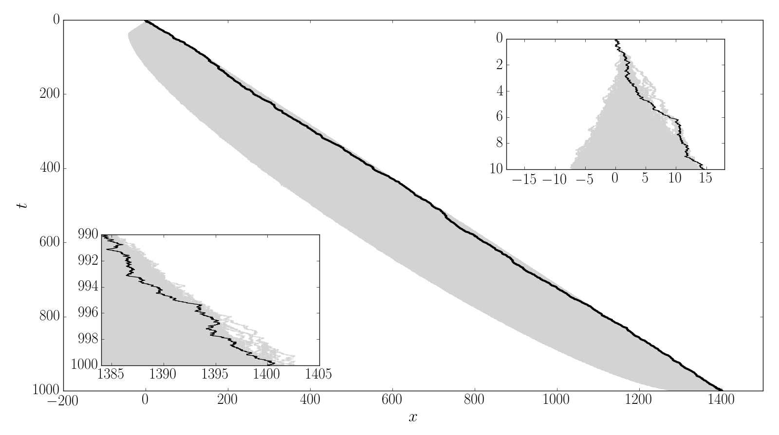
A realization produced with such an algorithm is sketched in Fig. 1. A realization actually generated, in the discretized version of the algorithm described in the next section, is displayed in Fig. 2.

Figure 1: Schematic evolution to time $T$ of a particle, starting at position $x$ at time $t$, through the branching Brownian motion conditioned to having at least one (“marked”) particle to the right of ${X_{\text{min}}}$ at $T$. The horizontal axis carries the space variable, the vertical one the time, which flows from top to bottom. The trajectory of this marked particle is represented by the thick full line. Its offspring may a priori end up at any position. The branchings that generate particles at position not smaller than ${X_{\text{min}}}-\Delta x$ are denoted by black disks, while the ones that generate only particles with smaller positions are denoted by circles. The trajectories of the latter are represented by dashed lines.

2.2 Discrete model

Although the algorithm described above can in principle be directly implemented, in practice, it is quite challenging to achieve a good accuracy. The reason is that a solution to the continuous FKPP equation is needed, potentially at any point in space-time. Such a solution can be obtained numerically only in an approximate way, by discretizing the FKPP equation on a lattice. Thus it is natural to start from the beginning with a discrete model in space and time, in such a way that the solution to the corresponding discretized FKPP equation directly provides the exact (up to machine accuracy) probabilities of the elementary processes involved.

We consider the following model discrete in space and time on a lattice with respective spacing $\delta x$ and $\delta t$: To evolve from $t$ to $t+\delta t$, a particle at $x$ may jump to $x-\delta x$ with probability $p_{l}$ or to $x+\delta x$ with probability $p_{r}$ (these two processes define a random walk), or may stay at the same position but split to two particles with probability $p_{b}$. The choice of the parameters of the model is constrained by the unitarity relation $p_{l}+p_{r}+p_{b}=1$ which must be imposed, together of course with the restriction of each of these elementary probabilities to the interval $[0,1]$.

The detailed implementation of this model depends on the observable we want to measure. We are first going to briefly show how to implement a full unbiased evolution, and then describe the method to generate ensembles of “long-tail” realizations in which there is at least one particle in the interval $[{X_{\text{min}}},+\infty[$ at the final time $T$.

2.2.1 Generating unconditioned realizations

At time $t$, the system is fully characterized by the set of the numbers of particles $\{n(t,x)\}$ on all occupied sites. The evolution of the system between the times $t$ and $t+\delta t$ goes as follow: Among the $n(t,x)$ particles on site $x$ at time $t$, there are $n_{l}(t,x),n_{r}(t,x)$ particles that move on the site to the left and to the right respectively, and $n_{b}(t,x)$ particles that duplicate, with the sum rule $n_{l}+n_{r}+n_{b}=n$. The numbers $(n_{l},n_{r},n_{b})$ are distributed according to the multinomial law

$$\text{proba}(n_{l},n_{r},n_{b}=n-n_{l}-n_{r})=\frac{n!}{n_{l}!\,n_{r}!\,(n-n_{l}-n_{r})!}\,p_{l}^{n_{l}}p_{r}^{n_{r}}(1-p_{l}-p_{r})^{n-n_{l}-n_{r}}.$$ (9)

On the sites on which $n$ is very large compared to unity, the stochastic evolution can safely be replaced by the mean-field deterministic evolution.

The numbers $\{n_{l}(t,x),n_{r}(t,x),n_{b}(t,x)\}$ are drawn randomly according to the law (9) at each time step, except on the sites on which $n(t,x)$ is very large, in which case the numbers $n_{l}(t,x)$, $n_{r}(t,x)$ and $n_{b}(t,x)$ are just proportional to $n(t,x)$, with respective coefficients $p_{l}$, $p_{r}$ and $p_{b}$ (“mean field” approximation). In any case, for each new iteration, the CPU time is proportional to the number of occupied sites, which is a stochastic variable the mean of which grows linearly with the evolution time. Hence the overall complexity grows quadratically with the final time $T$. The memory occupancy depends on the observable. It is linear in $T$ for the observables of interest in this work, for which we just need to record the particle content at the current time.

2.2.2 Conditioned ensembles

Long-tail events are (arbitrarily) rare, so it is not possible to build a large statistical ensemble of such realizations using the full Monte Carlo we have just described. It is however possible to write an exact Monte Carlo that generates only events which have at least one particle with position not smaller than ${X_{\text{min}}}$ at the final time $T$. We can generate complete realizations, that is to say, keep all the particles until the final time; We can also evolve only the particles that end up at positions not smaller than say ${X_{\text{min}}}-\Delta x$ at time $T$, which is actually enough if the purpose is to study the tip of the particle distribution at the final time. We shall now describe the two versions of the algorithm in greater detail.

Complete realizations.

The initial particle is marked and conditioned to arrive at some position $x\geq{X_{\text{min}}}$. This ensures that in the realization, there is one or more particle(s) in that region. Its evolution is conditioned to having at least one particle in its descendence in that spatial region. As for the first step, which brings the marked particle from time $t$ to time $t+\delta t$, this conditioning is performed through the replacement of the probabilities $p_{l}$, $p_{r}$ of the elementary jump processes by

$$\begin{split}&p_{l}^{\prime}(T-t,{X_{\text{min}}}-x)\equiv p_{l}\times\frac{u(T-t-\delta t,{X_{\text{min}}}-x+\delta x)}{u(T-t,{X_{\text{min}}}-x)}\\ &p_{r}^{\prime}(T-t,{X_{\text{min}}}-x)\equiv p_{r}\times\frac{u(T-t-\delta t,{X_{\text{min}}}-x-\delta x)}{u(T-t,{X_{\text{min}}}-x)},\end{split}$$ (10)

and the branching probability by

$$p_{b}^{\prime}\equiv 1-p_{l}^{\prime}-p_{r}^{\prime}.$$ (11)

In these expressions, $u(\tau,\xi)$ is the probability of having at least one particle with position not smaller than $\xi$ at time $\tau$ starting with a single particle at position $\xi=0$ at time $\tau=0$. It solves an equation in the universality class of the FKPP equation that is straightforward to derive from the definition of the model,

$$u(\tau+\delta t,\xi)=p_{r}\,u(\tau,\xi-\delta x)+p_{l}\,u(\tau,\xi+\delta x)+p_{b}\,u(\tau,\xi)[2-u(\tau,\xi)],$$ (12)

with the initial condition

$$u(0,\xi)=1\quad\text{for $\xi\leq 0$},\quad u(0,\xi)=0\quad\text{for $\xi>0$}.$$ (13)

Using the probabilities $p^{\prime}_{l}$, $p^{\prime}_{r}$, $p_{b}^{\prime}$, one chooses among the three possible outcomes of the evolution between times $t$ and $t+\delta t$: The particle moves left, or moves right, or branches. As before for the BBM, there are two main cases to distinguish:

• If no branching occurs, the position of the marked particle is just updated from $x$ to $x\mp\delta x$, according to whether it jumps left or right. The next evolution step, to the time $t+2\delta t$, uses the biased probabilities $p^{\prime}_{l}$, $p^{\prime}_{r}$ and $p_{b}^{\prime}$ evaluated at the point $(T-t-\delta t,{X_{\text{min}}}-x\pm\delta x)$.

• If a branching occurs, then there is a second particle at position $x$ at time $t+\delta t$, in addition to the marked one. This new particle is evolved with the full unbiased algorithm described in the previous section 2.2.1 until the final time $T$, independently of the marked particle. The marked particle instead keeps evolving according to the biased probabilities $p^{\prime}_{l}$, $p^{\prime}_{r}$ and $p_{b}^{\prime}$, evaluated at $(T-t-\delta t,{X_{\text{min}}}-x)$.

Keeping only the particles close to the tip.

For our particular purpose in this paper, and actually for all studies which would focus only on the region near the lead particle, it is enough to keep track of the particles which have positions not smaller than ${X_{\text{min}}}-\Delta x$ at the final time $T$. Hence when a branching of the marked particle occurs, it is enough to keep the offspring only if it possesses at least one descendant with position not smaller than ${X_{\text{min}}}-\Delta x$ at the final time $T$.

The jumps of the marked particle keep the same probabilities as given in Eq. (10). The branching process of the marked particle is replaced by two processes: A branching may still occur, but with the probability

$$p_{b}^{\prime}(T-t,{X_{\text{min}}}-x)\equiv p_{b}\times u(T-t-\delta t,{X_{\text{min}}}-x)\\ \times\frac{2u(T-t-\delta t,{X_{\text{min}}}-\Delta x-x)-u(T-t-\delta t,{X_{\text{min}}}-x)}{u(T-t,{X_{\text{min}}}-x)},$$ (14)

which takes into account the new conditioning. But the marked particle may also just remain on its site $x$ without branching. This may occur with the probability

$$p_{s}^{\prime}\equiv 1-p^{\prime}_{l}-p^{\prime}_{r}-p_{b}^{\prime}.$$ (15)

When a branching of the marked particle takes place, while the evolution of the latter is just an iteration until the final time $T$ of the processes we have just described, the further evolution of the second particle is conditioned in such a way that it has at least one descendent which arrives at a position not smaller than ${X_{\text{min}}}-\Delta x$. Hence from the time $t+\delta t$ to $t+2\delta t$, it evolves according to the following processes: It may move left or right with respective probabilities

$$p_{l}^{\prime\prime}\equiv p^{\prime}_{l}(T-t-\delta t,{X_{\text{min}}}-\Delta x-x)\quad\text{and}\quad p_{r}^{\prime\prime}\equiv p^{\prime}_{r}(T-t-\delta t,{X_{\text{min}}}-\Delta x-x),$$ (16)

or branch to two particles (that both get further evolved) with probability

$$p_{b}^{\prime\prime}(T-t-\delta t,X-x)\equiv p_{b}\times\frac{\left[u(T-t-2\delta t,{X_{\text{min}}}-\Delta x-x)\right]^{2}}{u(T-t-\delta t,{X_{\text{min}}}-\Delta x-x)},$$ (17)

or else, do nothing, with probability

$$p_{s}^{\prime\prime}\equiv 1-p^{\prime\prime}_{l}-p^{\prime\prime}_{r}-p_{b}^{\prime\prime}.$$ (18)

By iterating these processes until the final time $T$ is reached, one only evolves the particles that end up at time $T$ with a position greater or equal to ${X_{\text{min}}}-\Delta x$, including a marked particle which ends up at a position greater or equal to ${X_{\text{min}}}$. This procedure leads to realizations of particle sets in the range of positions $[{X_{\text{min}}}-\Delta x,+\infty[$ at time $T$ distributed according to the exact probabilities. One particular realization generated by our code is shown in Fig. 2.

The main limitation of this algorithm is the size of the memory needed to store the solution to Eq. (12) (which may be traded for CPU time by partially recomputing $u$ when needed), which grows linearly with $T$.

Figure 2: Realization of the BRW defined in Sec. 2.2 and 3.1 evolved to $T=1000$ using the algorithm described in Sec. 2.2.2. Time flows from top to bottom. ${X_{\text{min}}}$ is set to 1400, and one keeps only the particles that end up at a position not smaller than $1300$. The grey zone represents the set of the space-time trajectories of all the particles that are evolved by the algorithm. The black continuous line represents the worldline of the marked particle, that is conditioned to end up at a position greater or equal to ${X_{\text{min}}}$ at time $T$. Insets: Zoom on the initial times $t\in[0,10]$ (upper right) and final times $t\in[990,1000]$ (lower left).

3 Probability distribution of particle numbers near the tip

We consider a BRW evolved from time 0 to time $T$. We denote by $X$ the position of the rightmost particle at $T$ in a given realization. The observable we are interested in is the probability distribution $p_{n}(\Delta x)$ of the number $n$ of particles in the interval $[X-\Delta x,X]$. The position $X$ can be let free, or can be constrained to be at least as large as some minimal value ${X_{\text{min}}}$.

3.1 Analytical expressions for a few observables

The analytical expressions for the typical and mean particle numbers involve the values of a few parameters that characterize the shape and velocity of the traveling wave which is known to solve asymptotically Eq. (12). We start by computing these parameters for the model we have implemented, and then, we briefly review the available analytical results.

3.1.1 Properties of the asymptotic solutions to the FKPP equation

The method to compute the parameters characterizing the asymptotic solutions to equations in the universality class of the FKPP equation is standard. We will not expose it in detail: Instead, we shall refer the reader to a review such as the one in Ref. [3].

One looks for solutions to the equation obtained by linearizing equation (12) near the fixed point $u=0$, using the Ansatz $e^{-\gamma[x-v(\gamma)t]}$. The velocity $v(\gamma)$ of the partial wave $e^{-\gamma x}$ reads

$$v(\gamma)=\begin{cases}\frac{\gamma}{2}+\frac{1}{\gamma}&\text{for the BBM}\\ \frac{1}{\gamma\delta t}\ln\left(p_{r}\,e^{\gamma\delta x}+p_{l}\,e^{-\gamma\delta x}+2p_{b}\right)&\text{for the BRW}.\end{cases}$$ (19)

While the linearized equation results in a (discretized) diffusion and an exponential growth of $u$ with time due to the branchings, the main effect of the nonlinearity present in Eq. (12) is to make sure that $u$ remains less than 1 by compensating for its exponential growth with time in the spatial regions in which $u\sim{\cal O}(1)$. The result of the joint action of the linear and nonlinear terms in Eq. (12) is the formation of a so-called “traveling wave”, namely a moving front smoothly connecting $u=1$ at $x=-\infty$ to $u=0$ at $x=+\infty$. The transition region between these asymptotics turns out to be located at the time-dependent spatial coordinate

$$m_{t}=v(\gamma_{0})t-\frac{3}{2\gamma_{0}}\ln t+\text{const},$$ (20)

up to terms that vanish in the limit $t\rightarrow+\infty$. In this formula, the additive constant depends on the very definition of the front position, the two other terms are universal. The constant $\gamma_{0}$ is the value of $\gamma$ which minimizes $v(\gamma)$. The wave front has the shape

$$u(t,x)\simeq\text{const}\times(x-m_{t})\,e^{-\gamma_{0}(x-m_{t})}\exp\left(-\frac{(x-m_{t})^{2}}{2\gamma_{0}v^{\prime\prime}(\gamma_{0})t}\right)$$ (21)

in the parametric region $1\ll x-m_{t}\lesssim\sqrt{\gamma_{0}v^{\prime\prime}(\gamma_{0})t}$ and for large times $t\gg 1$.

In practice, we set the parameters of the model as follows:

$$p_{r}=p_{l}=\frac{1}{2}(1-\delta t),\ p_{b}=\delta t,\quad\text{with}\quad\delta t=0.01,\ \delta x=0.1.$$ (22)

The minimization condition for the velocity function, $v^{\prime}(\gamma)|_{\gamma=\gamma_{0}}=0$, has the following solutions, in the two cases of interest in this paper:

$$\gamma_{0}=\begin{cases}\sqrt{2}&\text{for the BBM}\\ 1.4319525\cdots&\text{for the BRW}.\end{cases}$$ (23)

This constant sets the decay rate of the wave front at very large $t$ and for $x-m_{t}\gg 1$. The other model-dependent constants entering Eqs. (21),(20) read

$$v(\gamma_{0})=\begin{cases}\sqrt{2}\\ 1.3943622\cdots,\end{cases}\gamma_{0}\,v^{\prime\prime}(\gamma_{0})=\begin{cases}1&\text{for the BBM}\\ 0.96095291\cdots&\text{for the BRW.}\end{cases}$$ (24)

We may observe that with our choice (22), the particular BRW model we implement can indeed be seen as a discretization of the BBM with diffusion constant $\frac{1}{2}$ and replacement rate 1. As expected, the constants in Eqs. (23),(24) differ by a few percents between the BBM and the BRW, as an effect of the discretization in $t$ and $x$. Note that it is essential to take time steps of size $\delta t$ small compared to the inverse branching rate, although such choices make it more difficult to reach large times in the numerical calculation.

3.1.2 Characterizing analytically the particle number at the tip

We now review a few properties of the distribution of the particle number $n$ in the interval $[X-\Delta x,X]$ [8, 9].

Case in which $X$ is unconstrained.

In the case in which the realizations are not conditioned to the final position of the rightmost particle, the measure of the particle density as seen from the tip was shown to be a decorated Poisson process [8] (see also [15, 11, 16]). We shall denote by $p_{n}^{(0)}(\Delta x)$ the distribution of the number of particles in an interval $\Delta x$ from the tip, and $\bar{n}^{(0)}(\Delta x)$ its expectation value.

In the region $1\ll\Delta x\lesssim\sqrt{\gamma_{0}v^{\prime\prime}(\gamma_{0})T}$, the expectation value of $n$ scales like

$$\bar{n}^{(0)}(\Delta x)=\text{const}\times\Delta x\,e^{\gamma_{0}\Delta x}e^{-{\Delta x^{2}}/(2\gamma_{0}v^{\prime\prime}(\gamma_{0})T)}.$$ (25)

(The $T$-dependence in the r.h.s., which is a finite-$T$ correction going away for $T=+\infty$, is kept implicit in the l.h.s).

We may derive the shape of the distribution $p_{n}^{(0)}(\Delta x)$ from a simple picture. Let us define

$$Z_{T}\equiv\sum_{i=1}^{N(T)}[v(\gamma_{0})T-x_{i}(T)]e^{\gamma_{0}[x_{i}(T)-v(\gamma_{0})T]},$$ (26)

where $\{x_{i}(T),1\leq i\leq N(T)\}$ is the set of the positions of the $N(T)$ particles at time $T$ in the particular realization we are considering. According to the Lalley and Sellke theorem [18], for $T$ large, the $T$-dependent random variable $Z_{T}$ converges to a $T$-independent but realization-dependent positive number $Z$, with probability 1. Furthermore, there is a frame the origin of which is, at time $T$, at position

$$X_{T}=m_{T}+\frac{1}{\gamma_{0}}\ln Z+\text{const},$$ (27)

with respect to which the probability density of $X$ obeys the Gumbel distribution

$$\gamma_{0}\exp\left(-\gamma_{0}(X-X_{T})-e^{-\gamma_{0}(X-X_{T})}\right).$$ (28)

The additive constant in Eq. (27) is independent of the realization.

In this frame, the number of particles within the interval $[-\xi,0]$ (with $\xi>0$) in the realization grows like $\bar{n}^{(0)}(\xi)$, up to negligible fluctuations when $\xi$ is large enough. Hence the number of particles at a distance $\Delta x$ from the tip at position $X$ is proportional to $\bar{n}^{(0)}(\Delta x-X+X_{T})$. From the distribution (28) of $X-X_{T}$, we get, in the large-$T$ and large-$\Delta x$ limit,

$$\text{proba}\left(\delta\equiv\ln\frac{n}{\bar{n}^{(0)}(\Delta x)}\right)=\exp\left({\delta-e^{\delta}}\right)\implies\text{proba}(n)=\frac{1}{\bar{n}^{(0)}(\Delta x)}\exp\left(-\frac{n}{\bar{n}^{(0)}(\Delta x)}\right).$$ (29)

In the picture we have used here, the fluctuations of the multiplicity $n$ just reflect the fluctuations of the position of the lead particle in the Lalley-Sellke frame defined in Eq. (27).

Case in which $X-m_{T}$ is set large.

A few properties of the particle number distribution in the interval $[X-\Delta x,X]$ have been either computed or conjectured [9] in the joint limits $T\rightarrow+\infty$, $\Delta x\gg 1$, in the case in which the interval is included in the region in which the solution of the FKPP equation has reached its asymptotic shape $\propto(x-m_{T})\,e^{-\gamma_{0}(x-m_{T})}$, namely in which the Gaussian factor that exhibits an explicit $T$-dependence is very close to 1. This region is often called the “scaling region”: It extends over a distance of the order of $\sqrt{\gamma_{0}\,v^{\prime\prime}(\gamma_{0})\,T}$ to the right of the mean position $m_{T}$ of the rightmost particle.

As for the expectation value of $n$,

$$\bar{n}(\Delta x)=\text{const}\times e^{\gamma_{0}\Delta x},$$ (30)

up to finite-$T$ and finite-$\Delta x$ corrections that should vanish in the asymptotic limits. As for the typical value, the following conjecture was proposed:

$$n_{\text{typical}}=\text{const}\times\bar{n}(\Delta x)\times e^{-\zeta\Delta x^{2/3}},$$ (31)

again up to finite-$T$ corrections, and up to finite-$\Delta x$ corrections that might take the form of a linear prefactor.

The method to arrive at these results was based on the observation, derived from the discussion in Ref. [8], that a generating function of the particle number probabilities near the tip,

$$G_{\Delta x}(\lambda)=\sum_{n=1}^{\infty}\lambda^{n}p_{n}(\Delta x),$$ (32)

can be deduced from the solution to the FKPP equation with a peculiar $\lambda$- and $\Delta x$-dependent initial condition. The infinite-$T$ and large-$\Delta x$ behavior of the solution were then analyzed in two limits of the parameter $\lambda$ of the generating function: $\lambda\rightarrow 1$ and $\lambda\ll 1$ [9]. The former gives access to the mean particle number, while in the latter limit, a scaling form for $G$ was found, from which one could conjecture the behavior of the typical particle number [9].

3.1.3 Estimator of the typical value of the particle number

We need to specify what we mean by “typical value” of $n$ quantitatively.

With the reasonable assumption (well-verified numerically, see below) that $p_{n}(\Delta x)$ as a function of $n$ has a unique maximum, we may define it to be the mode of the distribution, that is to say, the value $n_{\text{typical}}^{\text{max}}$ of the particle number $n$ that maximizes $p_{n}(\Delta x)$. This number is obviously defined by the equation

$$\left.\frac{d}{dn}\right|_{n=n_{\text{typical}}^{\text{max}}}p_{n}(\Delta x)=0$$ (33)

when $n$ is large enough so that $p_{n}(\Delta x)$ can be considered a continuous (differentiable) function of $n$. But this is awkward when one works with statistical samples of moderate size: Therefore, we will not use this prescription in practice.

We have tried instead the median $n_{\text{typical}}^{\text{median}}$, defined by the equations

$$\text{proba}\left(n\leq n_{\text{typical}}^{\text{median}}\right)\geq\frac{1}{2}\quad\text{and}\quad\text{proba}\left(n\geq n_{\text{typical}}^{\text{median}}\right)\geq\frac{1}{2}.$$ (34)

Alternatively, we have used the expectation value of $\ln n$:

$$n_{\text{typical}}^{\text{log}}\equiv\exp\left({\langle\ln n\rangle}\right).$$ (35)

The latter is a good estimator of the typical value of $n$ for distributions which are symmetric in a logarithmic scale for $n$. Empirically, this turns out to be the case for the distribution of $n$ when the tip is conditioned to be far from its typical or mean position.

3.2 Numerical results

We now use the code we have developed in order to test numerically the formulae in Sec. 3.1 in the case of the discrete model described in Sec. 2.2.

The calculations/conjectures we want to test are actually valid for $T\rightarrow+\infty$, which, needless to say, can never be achieved numerically. What we can do instead is to test how the asymptotics is approached by performing calculations for different increasing values of the final evolution time $T$.

For each choice of the parameters ${X_{\text{min}}}$, $\Delta x$ and $T$, we need ensembles of a few thousands of realizations. With our algorithm and the state-of-the-art computer technology, the evolution time $T$ that may be reached within a few thousands hours of computer time is of the order of $10^{4}$.

For given ${X_{\text{min}}}$ and $T$, we actually measure observables for the different values of $\Delta x$ on the same samples of realizations. Hence these measurements are correlated.

3.2.1 Unconstrained realizations

We first let the position $X$ of the rightmost particle unconstrained. We shall nevertheless use the algorithm described above but with ${X_{\text{min}}}$ set to a value less than $m_{T}$, chosen in such a way that the probability to have no particle to the right of ${X_{\text{min}}}$ be negligible. The biasing has no effect on the observable since, with this procedure, $X$ is effectively unconstrained, but enables one to reduce the complexity of the numerical calculation.

Probability density.

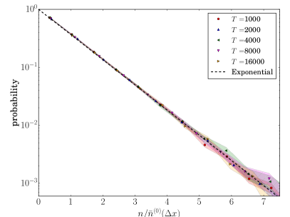
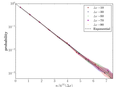
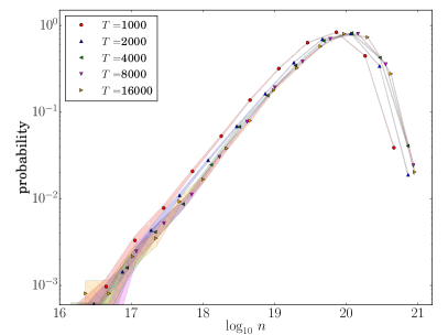
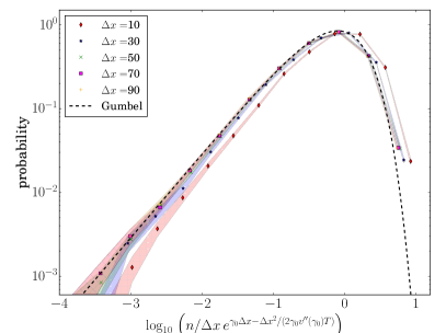
The distribution $p_{n}^{(0)}(\Delta x)$ of the number $n$ of particles in the interval $[X-\Delta x,X]$ is shown in Fig. 3. The points represent the probability of observing a given value of $n$ in bins of fixed size on the scale $n/\bar{n}^{(0)}(\Delta x)$. In this plot, the expectation value of the particle number is evaluated on the statistical ensemble. The error band is computed assuming Gaussian uncertainties in each bin.

We see that all the data points, either for fixed $\Delta x=30$ and different values of $T$ (Fig. 3a) or for fixed $T=8000$ and different values of $\Delta x$ (Fig. 3b), fall on the same exponential curve, and are thus perfectly consistent with Eq. (29).

(a)	(b)

Figure 3: Probability distribution of the number $n$ of particles in an interval of size $\Delta x$ to the left of the lead particle, at time $T$. The particle number $n$ is normalized by its expectation value $\bar{n}^{(0)}(\Delta x)$, computed numerically using the available data. (a) $\Delta x=30$ and different values of the evolution time $T$. (b) $T=8000$ and different interval sizes $\Delta x$. The dashed line represents the exponential $e^{-n/\bar{n}^{(0)}(\Delta x)}/\bar{n}^{(0)}(\Delta x)$.

For future comparison with the case in which ${X_{\text{min}}}$ is set large, it is useful to also plot the distribution of the logarithm of the particle number $n$. This is displayed in Fig. 4. We see that the data is independent of $\Delta x$ for large $\Delta x$, and is consistent with the analytic form given in Eq. (29). Indeed, the curve representing the distribution

$$\frac{\ln 10}{c}10^{\delta}\exp\left(-\frac{1}{c}10^{\delta}\right)\quad\text{with}\quad\delta\equiv\log_{10}\frac{n}{\Delta x\,e^{\gamma_{0}\Delta x-\Delta x^{2}/(2\gamma_{0}v^{\prime\prime}(\gamma_{0})T)}}$$ (36)

fits very well the numerical data when the constant $c$ is set to 0.8.

As a consequence of the shape of the multiplicity distribution, the typical and the mean values of $n$ are both proportional to $\Delta x\,e^{\gamma_{0}\Delta x}$, supplemented by the expected finite-$T$ correction factor $e^{-\Delta x^{2}/(2\gamma_{0}v^{\prime\prime}(\gamma_{0})T)}$.

(a)	(b)

Figure 4: Probability distribution of the logarithm of the particle multiplicity in an interval of size $\Delta x$ to the left of the lead particle, at time $T$. (a) $\Delta x=30$ and different values of the evolution time $T$. (b) $T=8000$ and different interval sizes $\Delta x$; The $x$-axis is translated by a term proportional to the expected mean particle number. The dashed line represents the theoretical probability (36) obtained in the simple picture explained in the text, with one free numerical constant of order 1 set by hand.

Mean and typical values.

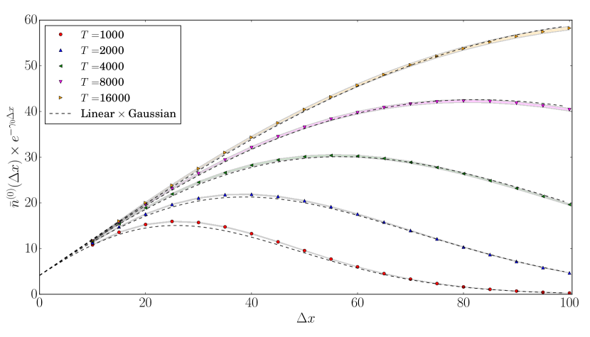
The mean value of the particle number, rescaled by $e^{-\gamma_{0}\Delta x}$, is shown in Fig. 5 as a function of $\Delta x$, for different values of $T$. The error band is evaluated using the jackknife method.

To the data, we superimpose the curves

$$\bar{n}^{(0)}(\Delta x)\times e^{-\gamma_{0}\Delta x}=\bar{c}(\Delta x+\bar{a})\exp\left(-\frac{(\Delta x+\bar{a})^{2}}{2\gamma_{0}v^{\prime\prime}(\gamma_{0})T}\right)$$ (37)

where the normalization $\bar{c}$ is not computable and hence has to be fitted, and $\bar{a}$ is a fudge term meant to effectively take into account some subleading corrections. We determine these constants using the data for $T=8000$. The best fit is obtained for the values $\bar{c}\simeq 0.80$ and $\bar{a}\simeq 5.2$. Note that the value of $\bar{c}$ fitted here is identical to the value of $c$ chosen to describe the data for the probability distribution $p_{n}^{(0)}(\Delta x)$ (see Eq. (36) and Fig. 4).

We see in Fig. 5 that the numerical data is consistent with this formula. In particular, for the largest value of $T$, the linear factor in Eq. (37) which encodes the expected asymptotics clearly becomes dominant.

Figure 5: Mean value of the particle number as a function of $\Delta x$, for different values of the evolution time $T$. The dotted curves represent the expected shape in the limit of large $T$ and $\Delta x\gg 1$, up to two free constants, see Eq. (37).

3.2.2 Long-tail realizations

We now constrain the position of the lead particle to be larger than ${X_{\text{min}}}$, chosen far from its expectation value, but in the scaling region. One may think of different prescriptions for the choice of ${X_{\text{min}}}$. We have decided to set the value of the diffusion factor, the width of which defines the size of the scaling region (see Eq. (21)), to a definite value $\alpha$. Namely:

$$\exp\left({-\frac{(X_{\text{min}}-m_{T})^{2}}{2\gamma_{0}v^{\prime\prime}(\gamma_{0})T}}\right)\equiv\alpha.$$ (38)

The constant $\alpha$ has to be picked such that $X_{\text{min}}-m_{T}$ may be large, and at the same time, $X_{\text{min}}$ sit well inside of the scaling region. This means that $\alpha$ must be close to 1, but not too close to allow for a wide-enough region ahead of the position $m_{T}$ for finite $T$. We have tested different values, and eventually picked $\alpha=0.9$ to get the main results discussed in this paper. The distance ${X_{\text{min}}}-m_{T}$, which gives the order of magnitude of the maximum value of $\Delta x$ for which our numerical calculation may be expected to turn out close to the large-$T$ asymptotics, are shown in Tab. 1 for different values of $T$.

$T$	1000	2000	4000	8000	16000
${X_{\text{min}}}$	1400	2800	5600	11185	22350
$X_{\text{min}}-m_{T}$	14.23	20.12	28.46	40.25	56.92

Table 1: Evolution times $T$ and values of the miminum position ${X_{\text{min}}}$ of the marked particle at $T$ used for our numerical calculations. ${X_{\text{min}}}$ is set so that $\alpha\simeq 0.9$. In each case, ${X_{\text{min}}}-m_{T}$ is also shown: It represents the typical maximum value of the size $\Delta x$ for which the interval $[{X_{\text{min}}}-\Delta X,{X_{\text{min}}}]$ may be considered included in the scaling region.

In each realization, we count the number of particles between the position $X$ of the rightmost one, and the position $X-\Delta x$. $X$ and ${X_{\text{min}}}$ do not necessarily coincide, and in general, they do not. But the ensemble of events is dominated by realizations in which the rightmost particle is at a distance of order unity to the right of the position ${X_{\text{min}}}$, because the events in which $X$ is far from ${X_{\text{min}}}$ are probabilistically disfavored: Indeed, they are suppressed by a factor of the order $e^{-\gamma_{0}(X-{X_{\text{min}}})}$ if $X$ is still in the scaling region, and by an additional Gaussian factor if $X$ gets outside of the scaling region. Since we always count the particles in an interval of fixed size from the rightmost particle, the particle numbers have no reason to get enhanced in the realizations is which $X$ is larger than usual. Therefore, the fact that the position of the lead particle is not exactly fixed cannot affect significantly the observables studied in this paper.

Probability density.

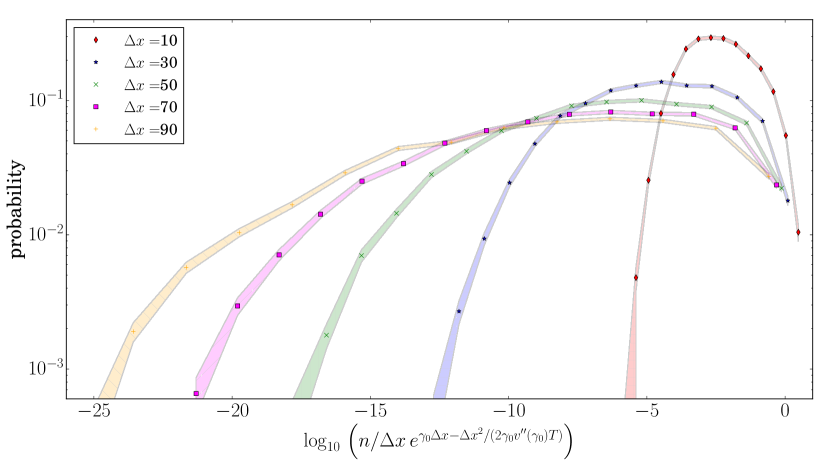
The distribution of the particle number $p_{n}(\Delta x)$ is shown in Fig. 6, for three different values of $\Delta x$, for different values of the final evolution time $T$. For each choice of $T$, ${X_{\text{min}}}$ is set as shown in Tab. 1.

Figure 6: Probability distribution of the number $n$ of particles in an interval of size $\Delta x$ for different values of $\Delta x$ and of the evolution time $T$. The lower bound ${X_{\text{min}}}$ on the position of the lead particle is chosen in such a way that $\alpha\simeq 0.9$, see Tab. 1.

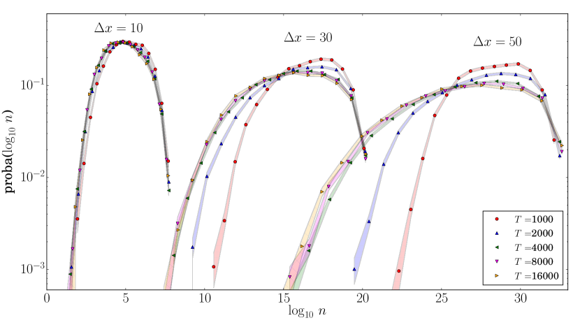
First, we observe that when $T$ gets large, the distributions converge to an asymptotic shape for all values of $\Delta x$. The convergence is faster for small interval sizes $\Delta x$.

Second, for asymptotic values of $T$, which seem to be well-approached for the displayed values of $\Delta x$ as soon as $T\sim 10^{4}$, the width of the distribution $p_{n}(\Delta x)$ clearly increases with $\Delta x$, at sharp variance with $p_{n}^{(0)}(\Delta x)$ (see Fig. 4). This increase is particularly striking for the largest value of $T$ for which we collected numerical data, namely $T=16000$; See Fig. 7, where the probability distribution of the particle number for different values of $\Delta x$ is displayed, up to $\Delta x=90$. (Note however that for the largest values of $\Delta x$, the large-$T$ asymptotics have probably not been exactly reached.)

Figure 7: Probability distribution of the number $n$ of particles in an interval of size $\Delta x$ for $T=16000$ and different values of $\Delta x$; Compare to the equivalent plot for the unconditioned case displayed in Fig. 4b. The $x$-axis is shifted by the same $\Delta x$-dependent term (corrected by a $T$-dependent term, quite insignificant here) as in the latter figure, although in the present case, it does not match exactly with the logarithm of the mean value of $n$ we expect; See Eq. (30).

We shall now compute numerically the mean and typical values of this distribution.

Mean and typical values.

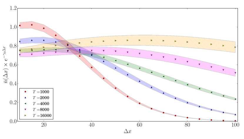
The numerical results for the expectation value of the particle number $\bar{n}(\Delta x)$ rescaled by $e^{-\gamma_{0}\Delta x}$ are shown in Fig. 8 as a function of $\Delta x$ for different values of the final evolution time $T$. The statistical uncertainties are again evaluated using the jackknife method.

We see that this rescaled expectation value is consistent with a constant independent of $\Delta x$ for large times (see the data for $T=16000$). This data is very different from the one in the unconstrained case; compare to Fig. 5.

Figure 8: Mean value of the particle number as a function of the interval size $\Delta x$, for different values of the evolution time $T$. The lower bound ${X_{\text{min}}}$ on the position of the lead particle is chosen in such a way that $\alpha\simeq 0.9$, see Eq. (38) and Tab. 1 for the actual numerical values.

The numerical results for the typical values of the particle numbers are shown in Figs. 9 and 10. We use the two estimators described in Sec. 3.1.3. We plot the ratio of the latter to the expectation values of the particle number, on a logarithmic scale, as a function of $\Delta x^{2/3}$.

We see a convergence to a straight line as the evolution time $T$ is taken larger. This is perfectly consistent with the expected behavior (31), namely $c\,e^{-\zeta\Delta x^{2/3}}$. The parameters $c$ and $\zeta$ are set to $c=2.2$ and $\zeta=0.86$ when the typical value is defined to be the median (Eq. (34)), and $c=3.3$ and $\zeta=0.92$ when it is defined to the exponential of the expectation value of $\ln n$ (Eq. (35)). Subleading corrections such as a linear prefactor $\propto\Delta x$ are not favored by the data. However, it is difficult to make more precise statements beyond the leading behavior, based on these finite-$T$ numerical results.

Figure 9: Ratio of the typical value of the particle number in the interval of size $\Delta x$ to the mean value as a function of $\Delta x^{2/3}$, for different values of the evolution time $T$. The theoretical expectation is shown in dashed line, with the free parameters $c$ and $\zeta$, for which no analytical formula is known to date, set arbitrarily (see the main text). In this plot, the typical value is taken to be the median, $n^{\text{median}}_{\text{typical}}$ (Eq. (34)). The dashed straight line represents the function $c\,e^{-\zeta\Delta x^{2/3}}$.

Figure 10: The same as in Fig. 9, but the typical value is now taken to be the exponential of the mean logarithm of the particle number, $n^{\text{log}}_{\text{typical}}\equiv e^{\langle\ln n\rangle}$ (Eq. (35)).

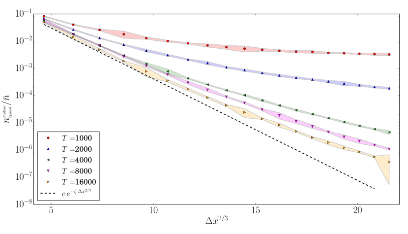
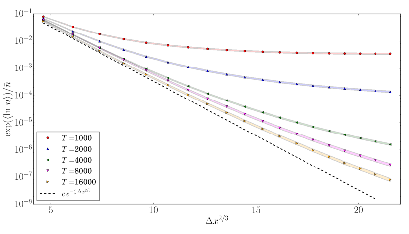
We note that finite-time (namely finite size of the scaling region) effects are important, and it is technically not possible to go much beyond $T={\cal O}(10^{4})$. However, it is clear that our numerical results are consistent with the analytical form that was predicted in Ref. [9].

4 Conclusions and outlook

We have designed an algorithm to efficiently generate realizations of branching random walks in which there is at least one particle to the right of some predefined position ${X_{\text{min}}}$ at the final time $T$ at which one analyzes the set of particles. Using an implementation of this algorithm, we have produced ensembles of such realizations for which ${X_{\text{min}}}$ was chosen in the scaling region, far to the right of the mean position $m_{T}$ of the rightmost particle. We have focused on the probabilities of the particle numbers $n$ in an interval of variable size $\Delta x$ to the left of the rightmost lead particle. The main result of this work is that we have been able to confirm a recent calculation of the mean number of particles $\bar{n}$, and a conjecture on the typical number of particles $n_{\text{typical}}$. They are seen to grow like

$$\boxed{\bar{n}(\Delta x)\propto e^{\gamma_{0}\Delta x}}\quad\text{(see Fig.~{}\ref{fig:mean_different_T})}\quad\text{and}\quad\boxed{n_{\text{typical}}\propto e^{\gamma_{0}\Delta x-\zeta\Delta x^{2/3}}}\quad\text{(see Fig.~{}\ref{fig:different_Ta} or~{}\ref{fig:different_Tb})}$$ (39)

with the size $\Delta x$ of the interval, when both the evolution time $T$ and $\Delta x$ are large.

This numerical result gives more motivation to look for a rigorous proof of these conjectures and for a formula for the probability distribution itself (Fig. 6 and 7), or at least for a complete analytical calculation in some simplified model. In parallel, a physical picture of the formation of these long tails would be interesting to develop, with the help of more specific Monte Carlo measurements.

The same algorithm could also be used to evolve unbiased realizations to large times: It is enough to pick ${X_{\text{min}}}$ to the left of $m_{T}$ by a distance chosen in such a way that the probability to have no particle to the right of ${X_{\text{min}}}$ be negligible. We could compare the distribution and its moments in the case when ${X_{\text{min}}}$ is far out in the scaling region, with same quantities in the case of an unconstrained boundary. In the latter case, the shape of the asymptotic distribution is independent of $\Delta x$ (see Fig. 4), and is consistent with a Gumbel distribution. The mean and typical values of the particle number are proportional to each other, and consistent with the asymptotic form $\bar{n}^{(0)}(\Delta x)\propto\Delta x\,e^{\gamma_{0}\Delta x}$; see Fig. 5.

A few other observables would be very interesting to measure numerically, with the help of our algorithm. For example, the statistics of the branching time of the last common ancestor of sets of particles chosen in the vicinity of the tip of the BRW according to given rules: For example, all particles to the right of a predefined position, or the $k$ rightmost, or a pair of particles chosen according to an appropriate weight function of their position. The considered realizations may be either unbiased, or conditioned to have their tip far from its expected position. Analytical predictions are available in some of these cases [24].

Another outstanding observable would be the mean distance between neighbouring particles possessing a predefined order number from the lead particle, as a function of the latter: This quantity has been predicted in the case of the branching Brownian motion with an unconstrained lead particle [25]. It would be interesting to measure this observable in an (effectively) unconditioned Monte Carlo and, again, investigate how it changes when the position of the rightmost particle is conditioned to be far from its expected value. But an implementation of the continuous BBM is very challenging. We leave this for future investigations.

Note added (June 29th, 2020)

A flaw in our algorithm has been brought to our attention, which may have introduced a bias in the probability distribution of the realizations we have generated.

After having corrected the algorithm [26] and reimplemented it, we have checked that the numbers obtained for the observables calculated with the new code are indistinguishable from the ones shown in this paper, in the case $T=1000$ and ${X_{\text{min}}}=1400$. In view of these first results, we anticipate that the conclusions we have drawn on $p_{n}(\Delta x)$ should eventually remain unchanged.

We will release a new preprint [27] when all the data, also for higher values of $T$, has been generated using the corrected code.

We warmly thank Éric Brunet for pointing out the problem to us, and for his prompt help in looking for a fix.

References

- [1] R. A. Fisher, “The wave of advance of advantageous genes,” Annals of Eugenics, vol. 7, no. 4, pp. 355–369, 1937.
- [2] A. Kolmogorov, I. Petrovsky, and N. Piscounov, “Étude de l’équation de la diffusion avec croissance de la quantité de matière et son application à un problème biologique,” Bull. Univ. État Moscou, vol. A 1, 1937.
- [3] W. van Saarloos, “Front propagation into unstable states,” Physics Reports, vol. 386, no. 2, pp. 29 – 222, 2003.
- [4] S. N. Majumdar, D. S. Dean, and P. L. Krapivsky, “Understanding search trees via statistical physics,” Pramana, vol. 64, p. 1175–1189, Jun 2005.
- [5] B. Derrida and H. Spohn, “Polymers on disordered trees, spin glasses, and traveling waves,” Journal of Statistical Physics, vol. 51, no. 5/6, 1988.
- [6] S. Munier, “Quantum chromodynamics at high energy and statistical physics,” Phys. Rept., vol. 473, pp. 1–49, 2009.
- [7] S. Munier and R. B. Peschanski, “Geometric scaling as traveling waves,” Phys. Rev. Lett., vol. 91, p. 232001, 2003.
- [8] É. Brunet and B. Derrida, “A branching random walk seen from the tip,” Journal of Statistical Physics, vol. 143, p. 420, Apr 2011.
- [9] A. H. Mueller and S. Munier, “Particle-number distribution in large fluctuations at the tip of branching random walks,” submitted to Phys. Rev. E, 2019.
- [10] C. Giardina, J. Kurchan, V. Lecomte, and J. Tailleur, “Simulating rare events in dynamical processes,” Journal of Statistical Physics, vol. 145, pp. 787–811, Nov 2011.
- [11] E. Aïdékon, J. Berestycki, É. Brunet, and Z. Shi, “Branching brownian motion seen from its tip,” Probability Theory and Related Fields, vol. 157, pp. 405–451, Oct 2013.
- [12] M. Bramson, “Convergence of solutions of the Kolmogorov equation to travelling waves,” Mem. Amer. Math. Soc., vol. 44, no. 285, pp. iv+190, 1983.
- [13] C. Graham, “Precise asymptotics for fisher–KPP fronts,” Nonlinearity, vol. 32, pp. 1967–1998, may 2019.
- [14] J. Berestycki, É. Brunet, and B. Derrida, “A new approach to computing the asymptotics of the position of fisher-kpp fronts,” EPL (Europhysics Letters), vol. 122, p. 10001, Apr 2018.
- [15] L.-P. Arguin, A. Bovier, and N. Kistler, “Poissonian statistics in the extremal process of branching brownian motion,” Ann. Appl. Probab., vol. 22, pp. 1693–1711, 08 2012.
- [16] L.-P. Arguin, A. Bovier, and N. Kistler, “The extremal process of branching brownian motion,” Probability Theory and Related Fields, vol. 157, pp. 535–574, Dec 2013.
- [17] A. H. Mueller and S. Munier, “Phenomenological picture of fluctuations in branching random walks,” Phys. Rev., vol. E90, no. 4, p. 042143, 2014.
- [18] S. P. Lalley and T. Sellke, “A conditional limit theorem for the frontier of a branching brownian motion,” Ann. Probab., vol. 15, pp. 1052–1061, 07 1987.
- [19] P. Maillard and M. Pain, “1-stable fluctuations in branching brownian motion at critical temperature i: The derivative martingale,” Ann. Probab., vol. 47, pp. 2953–3002, 09 2019.
- [20] E. J. Gumbel, “Les valeurs extrêmes des distributions statistiques,” Annales de l’institut Henri Poincaré, vol. 5, no. 2, pp. 115–158, 1935.
- [21] J.-P. Bouchaud and M. Mézard, “Universality classes for extreme-value statistics,” Journal of Physics A: Mathematical and General, vol. 30, p. 7997–8015, Dec 1997.
- [22] S. N. Majumdar, A. Pal, and G. Schehr, “Extreme value statistics of correlated random variables: A pedagogical review,” Physics Reports, vol. 840, p. 1–32, Jan 2020.
- [23] Z. Koba, H. Nielsen, and P. Olesen, “Scaling of multiplicity distributions in high energy hadron collisions,” Nuclear Physics B, vol. 40, pp. 317 – 334, 1972.
- [24] B. Derrida and P. Mottishaw, “On the genealogy of branching random walks and of directed polymers,” EPL (Europhysics Letters), vol. 115, no. 4, p. 40005, 2016.
- [25] É. Brunet and B. Derrida, “Statistics at the tip of a branching random walk and the delay of traveling waves,” EPL (Europhysics Letters), vol. 87, p. 60010, sep 2009.
- [26] Éric Brunet, Anh Dung Le, Alfred H. Mueller, S. Munier, “How to generate the tip of branching random walks evolved to large times,” arXiv:2006.15132 [cond-mat.stat-mech].
- [27] Éric Brunet, Anh Dung Le, Alfred H. Mueller, S. Munier, in preparation.