Architectures of Exoplanetary Systems. II: An Increase in Inner Planetary System Occurrence Toward Later Spectral Types for Kepler’s FGK Dwarfs
Abstract
The Kepler mission observed thousands of transiting exoplanet candidates around hundreds of thousands of FGK dwarf stars. He, Ford, & Ragozzine (2019) applied forward modeling to infer the distribution of intrinsic architectures of planetary systems, developed a clustered Poisson point process model for exoplanetary systems (SysSim) to reproduce the marginal distributions of the observed Kepler population, and they showed that orbital periods and planet radii are clustered within a given planetary system. Here, we extend the clustered model to explore correlations between planetary systems and their host star properties. We split the sample of Kepler FGK dwarfs into two halves and model the fraction of stars with planets (between 0.5–10 and 3–300 days), , as a linear function of the Gaia DR2 color. We confirm previous findings that the occurrence of these planetary systems rises significantly toward later type (redder) stars. The fraction of stars with planets increases from for F2V dwarfs to for mid K-dwarfs. About half () of all solar-type (G2V) dwarfs harbor a planetary system between 3 and 300 days. This simple model can closely match the observed multiplicity distributions of both the bluer and redder halves in our sample, suggesting that the architectures of planetary systems around stars of different spectral types may be similar aside from a shift in the overall fraction of planet hosting stars.
1 Introduction
NASA’s Kepler mission (Borucki et al., 2010, 2011a, 2011b; Batalha et al., 2013) boosted the number of strong exoplanet candidates by surveying stars for nearly four years. It revealed a large number of transiting super-Earth to sub-Neptune size planets () at short orbital periods ( yr) (Latham et al., 2011; Lissauer et al., 2011a, b; Howard et al., 2012; Lissauer et al., 2014; Rowe et al., 2014) and an abundance of tightly-spaced multitransiting planetary systems. These offer key clues about their architectures and formation histories (Ragozzine & Holman, 2010; Fabrycky et al., 2014; Winn & Fabrycky, 2015; He, Ford, & Ragozzine, 2019). In addition to enabling robust calculations of the planet population statistics themselves, the Kepler catalog also allows for the detailed study of the correlations between planetary systems and their host stars.
Many previous studies have used the census of exoplanet candidates from Kepler to infer the occurrence rates of planets around primarily main sequence stars of F, G, and K spectral types (Catanzarite & Shao, 2011; Howard et al., 2012; Fressin et al., 2013; Petigura, Marcy, & Howard, 2013b; Hsu et al., 2018; Mulders et al., 2018; Hsu et al., 2019; Zink & Hansen, 2019). Of these studies, Howard et al. (2012) was the first to report a dependence of the planet occurrence rate on host star spectral type. They used 1235 planet candidates (with orbital periods days) from the first three quarters of Kepler data (Borucki et al., 2011b), around dwarf stars spanning K, to explore how the occurrence of planets varies as a function of stellar effective temperature. By splitting the stellar sample into 500 K bins, they found a strong inverse relationship between the occurrence of small () planets and , for which they fit a linear model, where and . Interestingly, they did not find any such correlation for larger planets ().
In contrast, Fressin et al. (2013) found no dependence between planet occurrence and spectral type for the same planet sizes, using the first 16 quarters of the Kepler data containing planet candidates (Batalha et al., 2013) combined with a new model for the detection efficiency and accounting for false positives. They argue that the increase in planet occurrence toward later type stars is a result of observational bias, manifesting for three reasons: (1) the Kepler planet candidate list is incomplete for sub-Neptunes, such that many of these planets transiting the larger (earlier type) stars have not been recovered; (2) the distribution of planet radii rises towards smaller sizes, which are easier to detect around smaller (later type) stars; and (3) the false positive rate is slightly higher for later-type stars, artificially boosting the occurrence rate if not corrected for. In this work, we are able to address these concerns by taking advantage of more recent improvements in modeling Kepler’s detection efficiency (Burke & Catanzarite, 2017a, b, c; Christiansen et al., 2020; Coughlin, 2017), including accounting for the rate of false alarms due to instrument systematics and astrophysical false positives due to background blends and eclipsing binaries that can be recognized by the transit shape and/or pixel offset from the Robovetter and using the Kepler DR25 catalog that was vetted using this fully automated pipeline (Thompson et al., 2018). We show that the limit of transit detectability for a given planet is more complicated than what would result from only considering the stellar radius.
Mulders, Pascucci, & Apai (2015) extended the above studies to include a large sample of F, G, K, and M dwarfs, dividing these four spectral types using and computing the planet occurrence rates in each bin. With an eye toward exploring how the planetary system architectures, not just the overall rate of planets, may differ across stellar types, they calculated the occurrence rate as a function of semi-major axis for each spectral type. They find that the occurrence rate of planets between increases toward later spectral type at all separations out to days, in agreement with the findings of Howard et al. (2012). Mulders, Pascucci, & Apai (2015) also suggest that the cut-off semi-major axis (potentially indicative of the inner disk edge, where planets become less common interior of) shifts toward smaller separations for planets around later type stars.
Numerous studies have also constrained the occurrence of planets around M-dwarf stars, including those using surveys other than Kepler (e.g., Endl et al. 2006; Cumming et al. 2008; Gaidos et al. 2013; Bonfils et al. 2013; Lannier et al. 2016). The earlier works relied on radial velocity (RV) data and more massive planets, attempting to correct for survey completeness; for example, Cumming et al. (2008) used a sample of 585 FGKM stars with RV measurements and found that the occurrence of giant planets () within 2000 days around M-dwarfs is about an order of magnitude lower than that of FGK dwarfs. Similarly, Bonfils et al. (2013) also found a lower occurrence rate of giant planets around M-dwarfs compared to earlier type dwarfs, although at shorter periods days. Results from direct imaging are qualitatively consistent; Lannier et al. (2016) observed 58 M-dwarfs and inferred that giant planet companions (with masses and low mass ratios ) tend to be less common around low mass stars.
Returning to studies with the Kepler data, which mainly consists of smaller, super-Earth to sub-Neptune sized planets, Dressing & Charbonneau (2013) used a sample of stars then estimated to have K hosting 95 planet candidates to measure the occurrence rate of small planets (). Their results for the occurrence rates of small planets are generally larger than the values for FGK dwarfs found by other studies. Intriguingly, however, they find that the occurrence of planets () may actually increase from the cooler (mid) to hotter (early) M-dwarfs, although the number of planet candidates driving this result is relatively small (and they find no such trend for smaller planets with ). More recently, Hardegree-Ullman et al. (2019) also find an increased occurrence rate of planets around M-dwarfs, although with much larger uncertainties, as well as evidence for an increasing occurrence toward later M-dwarfs. The higher occurrence of small planets around M-dwarfs has also been suggested by Gaidos et al. (2016), who estimated an average of planets () per star between 1.5–180 days. Finally, Hsu, Ford, & Terrien (2020) and Bryson (2020) leveraged Kepler DR25, Gaia DR2, and 2MASS data to compute the planet occurrence rates around M-dwarfs. While their findings corroborate these previous results, they also show that the increased occurrence rates compared to that of FGK stars largely disappear when normalizing by stellar irradiance.
At the time of writing this paper, Yang, Xie, & Zhou (2020) also used the Kepler DR25 catalog of exoplanet candidates to study the occurrence of planetary systems, namely the fraction of stars with planets, as a function of stellar type. They split a sample of stars between 3000–7500 K into ten quantiles and modeled the fraction of stars with planets, the mean planet multiplicity, and the mutual inclination dispersion power-law index (assuming the same mutual inclination –planet multiplicity relation from Zhu et al. 2018, ) in each quantile. They also find that the fraction of stars with planets, and to a lesser significance the mean number of planets per system, increases with decreasing stellar effective temperature. In this paper, we take an approach similar to Yang, Xie, & Zhou (2020) to focus on the fraction of stars with planets as opposed to just the mean number of planets per star, as both of these quantities can be computed given knowledge of the intrinsic planet multiplicity distribution, which we constrain using our forward model. We extend the methodology described in He, Ford, & Ragozzine (2019) (hereafter Paper I) to explore a clustered model describing the relation between planetary architectures and host star properties, using Gaia colors as a proxy for stellar effective temperature (and equivalently, spectral type), where is a reddening correction. We summarize our forward modeling procedure in §2, focusing on the key features and updates while leaving the full details in Paper I (§2 therein). We model the fraction of stars with planets () as a linear function of for our FGK sample and show that the occurrence of planetary systems increases significantly toward later type stars. We also consider an alternative model in which the period power–law index () is a linear function of . In §3, we present our results for our new clustered models. We discuss the implications of our results in §4. Finally, we summarize our conclusions in §5.
2 Methods
As in Paper I (and described therein), our models are built in the context of the Exoplanets Systems Simulator (“SysSim”) codebase, which can be installed as the ExoplanetsSysSim.jl package (Ford et al., 2018b). Step-by-step instructions on how to install, as well as our forward models, can be accessed at https://github.com/ExoJulia/SysSimExClusters. The SysSim project is also described in Hsu et al. (2018, 2019).
Our previous models for planetary systems (non-clustered, clustered periods, and clustered periods and sizes models) and our multi-stage approach to performing an approximate Bayesian computing (ABC) analysis are fully described in Paper I. Here, we modify our best model, the clustered periods and sizes model, to explore the dependence on host star properties. In this section, we first summarize our full procedure and then describe the updates:
-
Step 0: Define a statistical description for the intrinsic distribution of exoplanetary systems.
-
Step 1: Generate an underlying population of exoplanetary systems (physical catalog).
-
Step 2: Generate an observed population (observed catalog) from the physical catalog.
-
Step 3: Compare the simulated observed catalog with the Kepler data.
-
Step 4: Optimize a distance function to find the best-fit model parameters.
-
Step 5: Explore the posterior distribution of model parameters using a Gaussian process (GP) emulator.
-
Step 6: Compute credible intervals for model parameters and simulated catalogs using ABC.
Our updates to each step are described in the following subsections.
2.1 Clustered Model Updates
In Paper I, we explored three models simulating planetary systems as a clustered Poisson point process and used forward modeling to fit to the key properties (e.g., marginal distributions of the principal observables for detected planets) of the Kepler planet catalog around a clean sample of FGK stars (Hsu et al., 2019). We found that the occurrence of multi-transiting systems, and their distributions of period ratios and radius ratios are highly clustered to the extent that a simple non-clustered model cannot reproduce. We showed that, instead, a model involving clustered periods and planet sizes provides the best fit to the observed data.
In this paper, we adopt this fully clustered model from Paper I and modify it slightly with a re-parametrization, before adding a dependence on the host star color. To review, our clustered periods and sizes model as described in Paper I consists of the following features:
-
Planet clusters: each planetary system is composed of “clusters” of planets. We attempt to assign a number of clusters drawn from a Poisson distribution (with mean parameter ), but some may be rejected due to stability concerns (see §2.2 of Paper I for the exact procedure). The number of planets for each cluster is drawn from a zero-truncated Poisson (ZTP) distribution (with mean parameter ).
-
Orbital periods: a power-law (with slope index ) describes the distribution of cluster period scales , and the period of each planet in the cluster is drawn from a log-normal distribution centred on with cluster width (where is the number of planets in the cluster and is a width scale parameter), between 3 and 300 days.
-
Planet radii: a broken power-law (with slope indices , , and break radius ) describes the distribution of cluster radius scales , and the radius of each planet in the cluster is drawn from a log-normal distribution centered on with cluster width , between 0.5 and . We note that this parametrization is not flexible enough to produce any radius valley.
-
Planet masses: a non-parametric, probabilistic mass–radius relation from Ning, Wolfgang, & Ghosh (2018) is used to draw the masses of the planets conditioned on their radii.
-
Eccentricities: the orbital eccentricities are drawn from a Rayleigh distribution (with scale ).
-
Mutual inclinations: two Rayleigh distributions for the mutual inclinations are used, corresponding to a high and a low mutual inclination population (with scales and , respectively, such that ), where the fraction of systems belonging to the high inclination population is .
-
Planets near resonance: peaks near the first-order mean motion resonances (MMRs) in the observed period ratio distribution are produced by drawing low mutual inclinations for the planets “near an MMR” with another planet (which we define as cases where the period ratio is in the range for any in {2:1, 3:2, 4:3, 5:4}), such that these planets have mutual inclinations drawn from the Rayleigh distribution with regardless of which mutual inclination population the system belongs to.
-
Stability criteria: adjacent planets are separated by at least mutual Hill radii, and orbital periods are resampled until this criteria is met. For clusters where a maximum number of resampling attempts has been met, the entire cluster is discarded. We note that for nominal (i.e. best-fitting) model parameters, of all attempted clusters are rejected, although this rate is greater for larger values of and . Thus in both Paper I and this paper, we also report the final (i.e. true) mean numbers of clusters and planets per cluster, which are more accurate than and respectively.
2.1.1 Modified clustered model: constant
The model described above induces a link between the way planets are distributed between clusters and the number of zero planet systems, since the number of clusters per system is drawn from a Poisson distribution which also controls the number of zero-cluster (and thus zero-planet) draws. In other words, the fraction of stars with planets in the above model (which we referred to as “FSWP” in Paper I) is the fraction of draws with at least one cluster that is successfully attempted (and thus is implicitly a function of ). To decouple these two, we modify the model by introducing an additional parameter, the fraction of stars with planets attempted , and replace the Poisson distribution for the number of clusters per system with also a ZTP. This way, controls the fraction of stars we draw planetary systems for, while and both parametrize the (ZTP-distributed) numbers of clusters and planets per cluster, respectively, for such systems. We call the fraction of stars with planets attempted because systems for which we draw planets can still end up with zero planets in the case where all planets are discarded after the maximum number of attempts due to the stability criteria, although this is very rare (% of attempted systems).
We make this modification to our clustered periods and sizes model from Paper I not only to decouple the number of zero–planet systems from the underlying multiplicity distribution, but also to serve as a baseline model for a more natural comparison to the new models we introduce below. For the remainder of this paper, we refer to this baseline model as the “constant ” model. While all of the model parameters are “constant” (i.e., not functions of stellar type) in this model, we use this name to differentiate from the models below in which or is dependent on the host stars.
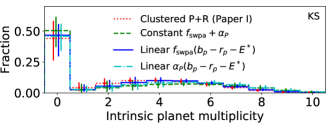
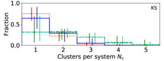
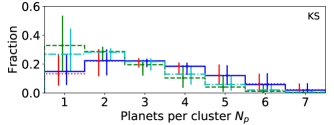
In Figure 1, we plot the intrinsic distributions of total planet multiplicity, clusters per system , and planets per cluster , for our old clustered model from Paper I (red dotted line) and our constant model (green dashed line). While our parametrization is different between these models, we find that the resulting intrinsic planet multiplicity distribution is very similar (top panel). We discuss these results in more detail in §3.1.
2.1.2 Model dependence on host star color
The occurrence of planetary systems is likely not independent of the host star properties (Howard et al., 2012; Dressing & Charbonneau, 2013; Mulders, Pascucci, & Apai, 2015; Hardegree-Ullman et al., 2019; Yang, Xie, & Zhou, 2020). As we motivate in §3, we find that while our clustered periods and sizes model performs well for our sample of Kepler planetary systems around FGK stars as a whole (Paper I), there are differences in the way these planets are distributed for different stars. These differences are complicated by the complex detection biases present in the Kepler survey. Since we are forward modeling planetary systems in detail using SysSim, our approach allows us to test various models in order to distinguish between these observational effects and real trends in the data.
In order to account for the potential differences in planet occurrence as a function of stellar properties, we introduce a host-star dependence in our clustered model. We adopt the cross–matched Gaia DR2 colors (Gaia Collaboration et al., 2018) as a proxy for spectral type, and we explore several model parameters as simple functions of color. We use the Gaia color instead of the more obvious choice of stellar effective temperature, , because of known limitations and caveats in the estimates of from Gaia DR2 photometry (Andrae et al., 2018). First, the characteristic scatter in relative to literature values is over 300K. In contrast, is measured precisely, as demonstrated by the narrowness of the main sequence in the versus color-luminosity diagram. Additionally, the small number of stellar models used for training by the Gaia team results in substantial “banding” of the inferred values. Indeed, we find three significant modes in the distribution of Gaia DR2 values for our sample. This would be particularly problematic for making precise comparisons of stellar temperatures. Therefore, we conclude that provides a superior proxy for making comparisons of the temperatures of stars within our particular stellar sample.
Stars in the Kepler field are moderately affected by reddening due to interstellar dust (Andrae et al., 2018); thus, we apply a correction for reddening. We find that there is a significant scatter in the reddening values of from Gaia DR2 for our Kepler target stars, and that the distribution of is trimodal, analogous to the values from Gaia DR2, and similarly due to the limited number of stellar models used. While the median is 0.15 mag, some targets have values as large as mag. Further, not all stars have valid values. Indeed, Andrae et al. (2018) caution that should not be used for individual stars, but advise that it be used for for statistical studies, such as this study. Therefore, instead of directly using the Gaia DR2 values for each star, we construct a simple model for as a function of by interpolation in order to account for differential reddening. While such an approach would not be wise for all science cases, it works well for the purposes of this study. First, for our analysis, we are only interested in the effects of differential reddening across a subset of the FGK main sequence stars observed by Kepler. The uncertainties due to differential reddening are significantly smaller for our sample than for Gaia targets in general. As explained below, we have applied multiple cuts to avoid stars that have evolved off the main sequence (e.g., subgiants, giants) as well as pre-main sequence or binary stars, so as to obtain a clean sample of FGK main sequence stars. The careful filtering of stars results in a smooth relation between Gaia color and reddening, after normalizing by distance.
Our procedure for applying a differential reddening correction is as follows. First, we perform all of the cuts described in Hsu et al. (2019) (see §3.1 therein) on the Kepler DR25 stellar catalog, which includes requiring targets to have:
-
•
a Gaia fractional parallax error less than 10%,
-
•
(for pre-selecting FGK stars), and
-
•
a luminosity , where is determined by iteratively fitting to the main sequence for the remaining stars, six times.
This results in 70,477 targets with Gaia–derived values. Then, we bin the stars into 20 quantiles by (about stars, or 5%, in each bin). While there is large scale structure to the distribution of interstellar dust as a function of galactic latitude, the primary Kepler field is highly localized, and we do not find that including galactic latitude makes a significant difference. Thus, main sequence stars of a similar spectral type or color at a similar distance should experience similar reddening. We compute the median distance–normalized reddening, where is the distance and is the parallax, for each bin. Although more reliable distances can be obtained using a probabilistic model (e.g., Bailer-Jones et al. 2018), our inversion of the parallax yields good distance estimates for our sample of target stars with small parallax uncertainties and thus strongly peaked likelihoods. The estimated distance–normalized reddening for each target is then computed by interpolating as a function of . Finally, we multiply by the distances again to get the interpolated reddening for each target, which we denote as . For the remainder of this paper, we will simply refer to the interpolated reddening values as , and likewise the colors corrected using the interpolated reddening values as (i.e., a measure of the intrinsic stellar colors). We note that the main analyses in this paper were also performed on the measured colors without a reddening correction (i.e. ) and the results are very similar, indicating that the results are insensitive to our choices for modeling colors and reddening.
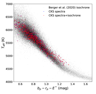
With our model for estimating as a smooth function of , we then apply the reddening correction to all target stars before the color and luminosity cuts described earlier. We re–cut and re–fit the FGK main sequence using the corrected colors, with . This results in a final stellar catalog of 88,912 usable targets (this is greater than the 70,477 targets before applying our interpolated reddening values because we also apply our reddening model to targets without Gaia values). The median (corrected) color is mag, which is close to the solar value. In Figure 2, we plot our reddening–corrected color () versus stellar effective temperature () from both the Berger et al. (2020) catalog (photometrically derived, isochrone fitted using Gaia DR2 data) and the California–Kepler Survey (spectroscopically derived; Johnson et al. 2018). There is a strong correlation between our corrected colors and the stellar temperatures.
2.1.3 Linear model
A simple way to allow for planet occurrence to vary with host star color in our clustered model is to allow the fraction of stars with planets, , to be a function of . This is simpler than allowing for the multiplicity to vary with stellar color, since in our clustered models we have two parameters controlling the number of planets per planetary system, and . In this model, we assume the form of a linear relation between and :
| (1) | ||||
where is the slope of the line, and is the -intercept (which we have chosen to parametrize at the median color, mag). We enforce to be bounded between 0 and 1, since the fraction of systems with planets cannot be negative or greater than 1. We refer to this model as the “linear ” model. Our previous (constant) model is essentially a special case of this more general model, where the slope is set to .
The blue solid lines in Figure 1 show the intrinsic planet and cluster multiplicity distributions for this linear model. While the fraction of stars with planets (and thus the fraction of zero-planet systems) is a strong function of host star color as we will show in §3, the intrinsic planet multiplicity distribution marginalized over all of the FGK stars in our sample is very similar to that of our baseline model (constant ; green dashed line). There is a slight tradeoff between the distributions of the number of clusters and planets per cluster compared to the constant model. We emphasize that the numbers of clusters and planets per cluster are not host star dependent since we have not made or functions of .
To serve as a check on this model, we also explore a “step ” model in which two parameters, and , describe the fraction of stars with planets below and above the median respectively. We briefly discuss the results for this model in §3.3.
2.1.4 Linear model
Another way in which planetary systems can differ as a function of host stellar type is in their distribution of orbital periods. For example, Mulders, Pascucci, & Apai (2015) found that the occurrence rate of small planets increases with decreasing stellar effective temperature at all semi-major axes less than 1 AU. Another motivation for exploring the “linear ” model is because it can have a similar effect as the fraction of stars with planets on the overall rate of detected planets, as a function of stellar color. We explore the period distribution in a similar way as the fraction of stars with planets, by allowing the period power-law index to vary as a linear function of :
| (2) | ||||
where is the slope and is the value at the median color.
2.2 Observational Comparisons
We adopt the same procedure for constraining our model parameters as described in Paper I, by defining a similar set of summary statistics and a distance function that accounts for these summary statistics.
2.2.1 Summary statistics
Since we are interested in how planet occurrence varies as a function of stellar color, we divide the stellar sample into two halves, split at the median color (a “bluer” half, with smaller values, and a “redder” half, with larger values). We compute the same summary statistics for each half, in addition to the full sample (hereafter labeled as “All”), for each observed catalog:
-
1.
the total number of observed planets relative to the number of target stars , ,
-
2.
the observed multiplicity distribution, , where is the number of systems with observed planets and ,
-
3.
the observed orbital period distribution, ,
-
4.
the observed period ratio distribution, ,
-
5.
the observed transit depth distribution, ,
-
6.
the observed transit depth ratio distribution, ,
-
7.
the observed transit duration distribution, ,
- 8.
The list above contains nine summary statistics, which we compute for each full observed catalog as well as for each of the bluer and redder halves, totaling 27 summary statistics.
2.2.2 Distance function
| Distance term | All | Bluer | Redder | |||
|---|---|---|---|---|---|---|
| 0.00103 | 971 | 0.00146 | 683 | 0.00154 | 649 | |
| 0.00593 | 169 | 0.01150 | 87 | 0.01373 | 73 | |
| : | ||||||
| 0.02616 | 38 | 0.03544 | 28 | 0.03805 | 26 | |
| 0.04836 | 21 | 0.06441 | 16 | 0.07167 | 14 | |
| 0.02907 | 34 | 0.03988 | 25 | 0.04121 | 24 | |
| 0.05106 | 20 | 0.06821 | 15 | 0.07437 | 13 | |
| 0.02831 | 35 | 0.03928 | 25 | 0.03995 | 25 | |
| 0.11572 | 9 | 0.16131 | 7 | 0.17897 | 6 | |
| 0.05607 | 18 | 0.07361 | 14 | 0.08078 | 12 | |
| : | ||||||
| 0.00113 | 882 | 0.00218 | 459 | 0.00233 | 429 | |
| 0.00329 | 304 | 0.00602 | 166 | 0.00736 | 136 | |
| 0.00138 | 723 | 0.00263 | 380 | 0.00276 | 362 | |
| 0.00392 | 255 | 0.00698 | 143 | 0.00862 | 116 | |
| 0.00145 | 691 | 0.00291 | 344 | 0.00302 | 331 | |
| 0.02098 | 48 | 0.04515 | 22 | 0.05154 | 19 | |
| 0.00479 | 209 | 0.00808 | 124 | 0.00982 | 102 | |
Note. — Each weight is computed as the inverse of the root mean square of the distances between repeated realizations of the same (i.e. “perfect”) model, , using the same number of target stars as our Kepler sample. The weights are shown here as rounded whole numbers for guidance purposes only.
In Paper I, we used a linear weighted sum of individual distance terms to combine the fits to each summary statistic into a single distance function. Two separate distance functions were used for the analysis, with one adopting the two-sample Kolmogorov–Smirnov (KS; Kolmogorov 1933; Smirnov 1948) distance for each marginal distribution and the other adopting a modified version of the two-sample Anderson–Darling (AD; Anderson & Darling 1952; Pettitt 1976; see equations 23–24 in Paper I for our modification) statistic. Both distance functions included a term for the overall rate of planets (, where and likewise for Kepler) and the observed multiplicity distribution (, where are the number of “observed” systems in our models and are the number of expected systems from the Kepler data, for multiplicity bins ; see Cressie & Read 1984 and the discussion surrounding equation 19 in Paper I).
For this paper, we extend the distance function in the same way as the summary statistics, by computing the individual distance term corresponding to each summary statistic, for each of the bluer, redder, and full samples, and summing them using a set of weights .
| (3) | ||||
| (4) |
where and everything within the outer summation refers to the distances computed using the summary statistics in a given sample only. The distances within the inner summation are either KS or AD distances, where the summation is over the indices labeling the summary statistics (iii)–(viii). As in Paper I, we repeat the analyses of this paper using both KS and AD distances, to serve as an additional check for the consistency of our results. The KS (two-sample) distance is simply the maximum difference between two cumulative distributions and thus primarily compares the modes of the distributions, while the AD (two-sample) distance is an integral that more heavily weights the tails of the distributions. As shown in §3, the results are very similar between both analyses, and thus we focus our discussion on the results from the (easier to interpret) KS distance function for the remainder of the paper.
Old weights: In order to compute the weights in Paper I, a single reference catalog was generated (using a nominal set of model parameters for the clustered periods and sizes model, and the same number of targets as our Kepler sample) and 1000 repeated catalogs were simulated (with five times as many targets, to reduce stochastic noise) from the same (i.e. “perfect”) model. The summary statistics and distances were then computed for each of the 1000 catalogs compared to the reference catalog, and the weight for each distance term was taken as the reciprocal of the rms of that distance term, , where is the distance term, and is the rms. While the weights computed in this way are reasonable, we find that they are prone to stochastic noise, even with larger numbers of repeated catalogs, since this method essentially treats one realization of the “perfect” model as the true data (i.e., the one used as the reference catalog). Also, the use of five times the number of targets for the repeated catalogs inflates the weights, due to reduced Monte Carlo noise and thus smoother distributions of the summary statistics.
New weights: In this study we compute the weights in a revised manner to resolve both of the above points: we simulate 100 catalogs assuming a single model, each with the same number of targets as the Kepler sample, and then compute the individual distances for each unique pair of catalogs before computing the rms for each distance term. This way, each of the 100 realizations of the same model are treated equally, with no single catalog serving as the reference catalog (or equivalently, all of the catalogs serve as the reference catalog), and there are effectively more evaluations of each distance term.111With just 100 simulated catalogs, each distance term is computed times instead of 1000 as before. We find that the weights generated in this way are significantly more reliable, even with the reduced number of model evaluations. The rms distances and weights are listed in Table 1. We also use a set of best-fitting model parameters from Paper I for the reference catalog (the parameters are listed in the Table 1 caption).
2.2.3 The Kepler catalog
Our stellar catalog is described in §2.1.2, where we detailed our procedure for accounting for differential reddening. To summarize, it is derived from a series of cuts on the Kepler DR25 target list based on updated stellar parameters from Gaia DR2 (Gaia Collaboration et al., 2018) as explained in Hsu et al. (2019) (§3.1 therein), with some modification to account for differential reddening using interpolated reddening values (). The list of cuts also includes Gaia GOF_AL and astrometric excess noise to filter out targets with a poor astrometric fit. In combination with the main sequence luminosity fitting described in §2.1.2, this filters out likely close–in binary stars. This results in a clean sample of 88,912 FGK main sequence stars, with corrected colors ranging from ( F2V) at the bluest end to ( K7V) at the reddest end. The planet catalog is derived from the Kepler DR25 KOI table (only keeping planet candidates around stars in our stellar catalog), where we also:
-
1.
replace the transit depths and durations with the median values from the posterior samples in Rowe et al. (2015),
-
2.
replace the planet radii based on the transit depths and the updated Gaia DR2 stellar radii, and
-
3.
only keep planets in the period range days and planet radii range .
Our final Kepler planet catalog consists of 2216 planet candidates. Of these, 982 are around stars in our bluer sample and 1234 are around stars in our redder sample.
2.3 Model Optimization
We adopt the same multi-stage approach in Paper I for performing approximate Bayesian inference on our model parameters. Our forward model is complex and relatively expensive, taking s to generate a physical and observed catalog with the same number of targets as our Kepler catalog. The model is also stochastic, due to Monte Carlo noise and the finite catalog size, resulting in a noisy distance function even for repeated evaluations using the exact same model parameters. Finally, the parameter space we are optimizing over is large, even larger than that of our clustered periods and sizes model due to the introduction of the parameter for our constant model, and and for our linear model (and likewise for the linear model). Thus, we begin with an optimization stage before training and using a fast emulator for inference with ABC.
| Parameter | Constant | Linear | Linear | ||||||
|---|---|---|---|---|---|---|---|---|---|
| Optimizer | Emulator | Optimizer | Emulator | Optimizer | Emulator | ||||
| 0.2 | 0.2 | 0.2 | |||||||
| aaThis is for the clustered model with linear . | 0.2 | 0.2 | 0.2 | ||||||
| - | - | - | 1 | - | - | - | |||
| - | - | - | - | - | - | ||||
| - | - | - | - | - | - | ||||
| - | 1 | - | 1 | - | 1 | ||||
| - | 2 | - | 2 | - | 2 | ||||
| bbThis is for the clustered model with linear . | 1 | 1 | 1 | ||||||
| - | - | - | - | - | - | 1 | |||
| 1 | 1 | 1 | |||||||
| 1.5 | 1.5 | 1.5 | |||||||
| 0.02 | 0.02 | 0.02 | |||||||
| (∘) | 30 | 30 | 30 | ||||||
| (∘) | 1 | 1 | 1 | ||||||
| 0.2 | 0.2 | 0.2 | |||||||
| 0.1 | 0.1 | 0.1 | |||||||
Note. — We varied the parameters and separately in the optimization stage, while we trained and predicted on and during the emulator stage (since these transformed parameters, the sum and difference of the log-rates of clusters and planets per cluster, appear more Gaussian). The same values are used for both of the analyses involving the KS and AD distance terms.
2.3.1 Optimization stage
The first step in our procedure for model optimization involves passing the distance function given by equation 4 into a Ddifferential evolution optimizer from the “BlackBoxOptim” package.222https://github.com/robertfeldt/BlackBoxOptim.jl This package provides several algorithms for general optimization problems. We choose the “adaptive_de_rand_1_bin_radiuslimited” optimizer, which implements a population-based genetic algorithm to minimize the target fitness function (i.e. our distance function), and set the population size to four times the number of free model parameters. We run the optimizer for 5000 model evaluations, with targets per evaluation, saving the results (model parameters and distances) at each iteration. Finally, we repeat the optimization process 50 times for each model and distance function (KS or AD) combination, each with a different starting point in the parameter space. The search bounds for the model parameters are listed in Table 2.
For each model and distance function, the optimization stage results in a pool of model evaluations. We first rank-order these sets of model parameters by their evaluated distance, and keep every tenth point in the top points so that we have a wide range of parameters (i.e. points both close to and far from the minima found by each run) for training the GP emulator. After ranking, we re-evaluate the distances at each of these points by regenerating a new simulated catalog, in order to avoid the bias that would result in keeping smaller-than-average distances at these points due to the combination of the stochastic nature of our simulations and the mere process of ranking.
2.3.2 GP emulator stage
The evaluations of the full forward model during the optimization stage are then used to train an emulator, which can “predict” the outputs of the model (i.e. the distance function) given similar inputs (i.e. model parameters). For our emulator, we use a Gaussian process (GP) model (Rasmussen & Williams, 2006) that is described by a prior mean function and a covariance (i.e. kernel) function :
| (5) | ||||
| (6) |
where is the distance function we wish to model, (and ) are the model parameters, and are the hyperparameters of the kernel. The values of the hyperparameters are also listed in Table 2. In particular, determines the strength of correlation between points and also acts as the standard deviation of the Gaussian prior (i.e., for points far away from any training data, the emulator effectively returns draws from a Gaussian distribution with mean and standard deviation ), while are the length scales in each dimension over which points are correlated.
We choose a constant prior mean function, with a value that is set toward the higher end of the distances of the training points. In this way, emulated distances at points far away from any training points will be significantly worse than the best distances achievable by our model, while emulated distances will only be lower than the mean function if they are near training points and these points suggest that the model is good in the vicinity. In practice, we also find that the AD distance is significantly more sensitive to deviations from a perfect model than the KS distance; we thus set for the distance function involving KS distances, and for the distance function involving AD distances. We verify that our results do not change much with differing choices for the mean function, as long as it is well above the minimum distances found by the optimizer and the distance threshold for constructing the ABC posterior.
2.3.3 ABC for model inference
In order to compute the credible regions for the model parameters, we construct an ABC posterior distribution by using the emulator to predict the model at a large number of points and accept those that pass a distance threshold. These points are drawn from the prior, for which we assume a uniform distribution in the -dimensional box (with bounds based on inspection of the training points, as listed in Table 2). In this paper, our distance function given by equation 4 (KS or AD) includes 27 individual distance terms, weighted and summed such that even a perfect model results in a distance of . While the lowest distances found during the optimization stage set the best distance threshold possible for a given model, the emulator performs a weighted average of points, and it becomes exceedingly computationally expensive to accept points passing thresholds approaching such distances. Thus, we choose somewhat larger distance thresholds that result in an efficiency of roughly or better for the fraction of drawn points accepted (drawn uniformly in our box). This results in distance thresholds of and for our linear models (and slightly larger thresholds, and , for our constant model, since this is a worse model, as we will show in §3). We collect points with emulated distances passing the distance threshold to serve as the ABC posterior for the model parameters. For more detailed calculations, we also simulate the full forward model and require that both the emulated and true distances pass the distance threshold.
3 Results
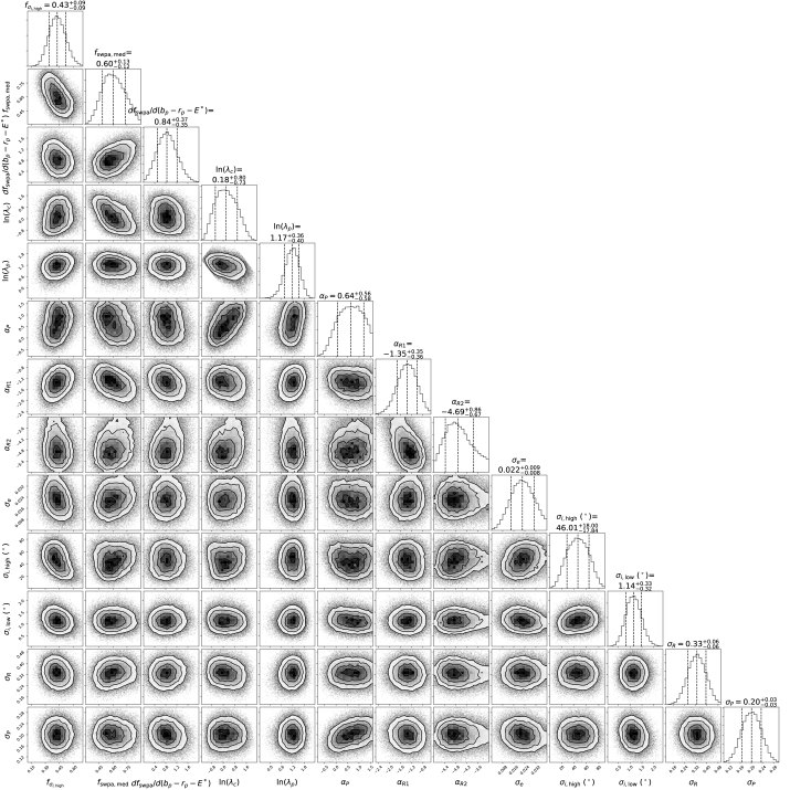
In this section, we first report and discuss the main results, beginning with a comparison to the clustered periods and sizes model in Paper I, before describing our findings for the model stellar dependence. In Table 3, we list the best-fitting values and 68.3% credible regions for the free parameters of the constant , linear , and linear models. We show the same credible regions (i.e. ABC posterior distributions) from our KS analysis in Figure 3 (linear model), supplemental Figure A2 (linear model), and supplemental Figure A1 (constant model). Our discussions will focus on the results from the KS distance function, as those from the AD distance function are very similar, except where noted (and both are listed in Table 3 for completeness).
| Parameter | Clustered P+R (Paper I) | Constant | Linear | Linear | ||||
|---|---|---|---|---|---|---|---|---|
| Best-fit KS | Best-fit AD | Best-fit KS | Best-fit AD | Best-fit KS | Best-fit AD | Best-fit KS | Best-fit AD | |
| aaThis is for the clustered model with linear . | - | - | ||||||
| - | - | - | - | - | - | |||
| bbThis is for the clustered model with linear . | ||||||||
| - | - | - | - | - | - | |||
| (∘) | ||||||||
| (∘) | ||||||||
Note. — While we trained the emulator on the transformed parameters and , we transform back to and to report the credible intervals. Unlogged rates and are shown for interpretability and are equivalent to the rows with log-values. The 68.3% credible regions are computed from the ABC posterior using distance thresholds of , 47, and 47 for the constant , linear , and linear models, respectively, in the KS analyses, while the distance thresholds are , 90, and 90, respectively, in the AD analyses.
3.1 The Overall Fraction of Stars with Planets
The only difference between our constant model and the clustered periods and sizes model in Paper I is a re-parametrization from a Poisson to a ZTP distribution for the number of clusters per system, with the addition of an explicit parameter for the fraction of stars with planets. As explained in §2.1.1, this change was made to (1) decouple the number of intrinsic zero-planet systems from the planet–hosting stars and their underlying multiplicity distribution and (2) produce a baseline model for comparison to our more general, linear (and linear ) model. Methodologically, we also used a distance function with three times the number of terms (fitting to the bluer half, redder half, and full samples) and recomputed weights, in order to facilitate a direct comparison with our new models. We first discuss how these results compare with the results from Paper I.
Fraction of stars with planets: For our baseline model, we find that the fraction of stars with planets (in our entire range explored, with periods between 3 and 300 days and planet radii between 0.5 and ) is well constrained. The KS and AD analyses result in similar values of and , respectively. These credible regions are also fully consistent with the results from the clustered periods and sizes model in Paper I, where the fraction of stars with planets in the same range is (via the KS analysis). This is noteworthy, given that we find a meaningful and comparable constraint on the despite a re-parametrization of the intrinsic multiplicity distribution and the extra dimensionality of the model optimization problem (and thus a larger parameter space).
Distribution of planets between and within clusters: While our baseline model and the clustered models from Paper I all have a parameter (for the mean rate of attempted clusters per planetary system), this parameter is not the same in these models. In Paper I, is the mean number of clusters per system before any rejection sampling and, due to the draws from a Poisson distribution, is also tied to the number of true zero-planet systems. Loosely, it could be interpreted as the mean number of clusters per star, including those that harbor no planets (between 3 and 300 days), although we found that the true mean is somewhat lower than what the parameter value suggests due to the rejected clusters. For our clustered periods and sizes model, about and of planet–hosting stars have just one and two clusters, respectively (Figure 1). Since the fraction of stars with planets in that model is , this means that the true mean number of clusters per system is about , where is the fraction of all stars with clusters, while the mean number of clusters per system with planets is .
In this paper, we have decoupled the parameter from the number of zero-planet systems and thus the fraction of stars with planets. However, we find that the mean numbers of clusters (and planets per cluster) are rather poorly constrained. For our constant model, we find that the mean rate of clusters per system is . Part of the reason we find such a large range of values is due to our algorithm for drawing planetary systems: as in Paper I, we draw clusters one by one, drawing their period scales after the unscaled periods for each planet in a cluster have been drawn, and only keeping clusters that can fit. In this manner, each individual cluster is deemed “stable” (given our minimum spacing in mutual Hill radii for adjacent planet pairs) before their period scale has been drawn, but the period scale drawn must also allow all of the planets in the cluster to be stable with the previously drawn clusters. As such, the actual number of accepted clusters can be significantly less than what would be suggested by the value of the parameter. Thus, we warn that our parameter values of (and ) should not be misinterpreted as the average number of clusters per system (or average number of planets per cluster). Instead, we count the true numbers of clusters and planets per cluster, as shown in Figure 1 for the KS analysis. The AD analysis (not shown) leads to somewhat more clusters per system and fewer planets per cluster, but a similar intrinsic planet multiplicity distribution (i.e. the top panel). We conclude that our decoupling of the parameter suggests that the true mean number of clusters per system is greater than what we found in Paper I, but the extent is unclear and is degenerate with the mean number of planets per cluster.
As noted earlier in §2.1.1, it is interesting that our re-parametrization of the intrinsic multiplicity distribution did not change the inferred distribution of total planet multiplicity in any noticeable way (i.e. compared to the red dotted line in the top panel of Figure 1). We also note that our intrinsic planet multiplicity distribution is very different than of that inferred by Sandford, Kipping, & Collins (2019), who found that a single Zipfian distribution (a discrete power-law distribution) that peaks at unity and falls off rapidly toward larger multiplicities best fits the observed Kepler counts. In contrast, our distribution peaks at a count of about four planets (for planet hosting stars), with similar fractions of seven-planet systems and one-planet systems. We attribute this difference to the constraints from the total rate of observed planets to stars and the fraction of stars with planets, which cannot exceed unity. In contrast, Sandford, Kipping, & Collins (2019) did not fit the rate of zero-planet systems (i.e. the fraction of stars with planets). As discussed in Paper I, we argue that the apparent excess of observed single–planet systems is unlikely to be due to a large fraction of true single–planet systems, since there are not enough stars available to host single planets to replace our high mutual–inclination population. These results highlight the importance of modeling the true fraction of stars with planets and simultaneously fitting the additional observables (period ratio distribution, and so on, as we have done here) when inferring the underlying multiplicity distribution, in order to distinguish between competing models for the Kepler dichotomy.
3.2 Planetary System Architectures
Broadly, we find consistent results for the model parameters describing the planetary system architectures between our new models and our old clustered periods and sizes model. We summarize the results here, quoting the KS results for our constant model. The results for our linear models and the AD results are listed in Table 3 and are very similar. For a more detailed discussion of what these parameters mean and comparisons to other values in the literature, see §3 of Paper I.
Period distribution (): the overall period distribution is described by a single power-law between 3 and 300 days, with a shallowly increasing occurrence in log–period given by .
Radius distribution (, ): the overall radius distribution is described by a broken power-law between 0.5 and , where we have set the break at . For planets below the break, the distribution is consistent with flat, ; above, there is a sharp fall-off with . As before, our models do not have the flexibility of producing a radius valley.
Eccentricity distribution (): we find small orbital eccentricities, described by a Rayleigh scale . While our models reproduce the transit duration and period-normalized transit duration ratio () distributions reasonably well, there may be evidence for a higher eccentricity component based on comparisons to the circular-normalized transit duration distribution (, where is the duration assuming a circular orbit with impact parameter ), although we have not included this distribution in our distance function for reasons described in §4.3.
Mutual inclination distribution (, , ): we still find clear evidence for a dichotomous population of planetary systems in terms of their mutual inclinations, with of systems assigned to the high mutual inclination population. We note that other solutions to the Kepler dichotomy exist (Zhu et al., 2018; Zink, Christiansen, & Hansen, 2019), but are beyond the scope of this paper. As in our models from Paper I (except where noted), in our new models we still draw mutual inclinations from for planets near an MMR with another planet, which affects about of all planets. The high mutual inclination scale , while clearly and significantly greater than , is still largely unconstrained at larger values since these systems primarily affect only the observed number of single-transiting systems, and our simple stability criteria do not directly account for the mutual inclinations. The low mutual inclination scale, degrees, suggests that most multi-planet systems are nearly but not exactly coplanar. This is consistent with our findings in Paper I and those of many previous studies, including Lissauer et al. (2011b) (who found an excellent fit to the multis with ), Fang & Margot (2012) (), and Fabrycky et al. (2014) (); see Section 3.6 in Paper I for a more detailed discussion.
Period and radius clustering (, ): the periods and planet radii of planets in the same cluster are each highly correlated. We find that , where this parameter quantifies the width per planet in the cluster for each cluster, in log-period. On the other hand, , which is the cluster scale in log-radius (regardless of the number of planets in the cluster). These two parameters are most directly constrained by the period ratio and transit depth (i.e. radius) ratio distributions, respectively.
3.3 Occurrence of Planetary Systems with Spectral Type
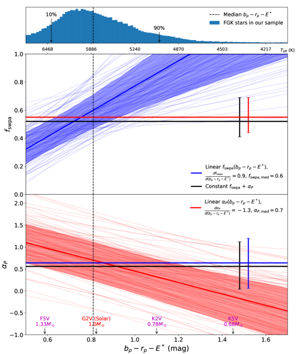
For the linear model (middle panel), the fraction of Sun-like stars with planets (between days and ) is around 60%. A few other example values are labeled with arrows (magenta), where we have used a table relating and from Pecaut & Mamajek (2013). The fraction increases by over a factor of two from the bluest (early F) to the reddest (late K) dwarfs in our sample. Alternatively, the linear model (bottom panel) exhibits a decrease in with increasing , corresponding to a shallower rise in occurrence toward longer periods for planets around redder stars (for reference, a value of corresponds to a flat distribution in log–period).
We find a significant positive slope for the linear relation between and color, suggesting that the occurrence rate of planetary systems between 3 and 300 days increases toward later type (redder, higher ) stars. The slope is () using KS (AD) analyses. Both analyses result in a similar slope and strongly disfavor a flat or negative slope. As expected, the fraction of stars with planets at the median color (), is comparable to the overall fraction of stars with planets (i.e. ) for our baseline model; we find that .
In Figure 4 (middle panel), we plot our best–fitting (KS) relations for the linear model. The solid blue line shows an example line that is close to the median relation, with and . We also plot 100 individual models, each passing our KS distance threshold, as light blue lines, and we denote the 68.3% credible region by the shaded blue region. The values of for the constant and linear models are also plotted as horizontal black and red lines with 68.3% error bars, respectively, for comparison. The distribution of for our stellar sample is plotted as a histogram in the top panel, with a vertical dashed line denoting the median value. We use the table from Pecaut & Mamajek (2013) to adopt a relation between Gaia color and stellar effective temperature , which we label as a secondary x-axis in Figure 4.
Given that our stellar sample ranges from to , the large slope for our linear relation suggests that the fraction of stars with planets changes by over a factor of two going from the bluest stars (early F dwarfs) to the reddest stars (late K dwarfs) in our sample. For F2V dwarfs, , while this value increases to for mid K dwarfs. The rises to unity beyond ( K), implying that inner planetary systems are extremely common around cooler stars. A more complex model than a simple linear relation may be necessary to model differences at this range of stellar types. We also note that while we assume a linear relation, we fit it using two samples split at the median stellar color, around which most of our stars are concentrated. Finally, the fraction of solar-type (G2V) dwarfs harboring at least one planet between 3 and 300 days is , or roughly half.
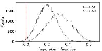
Step model: As a check on the results of our linear model, we also explore a model in which the fraction of stars with planets is set to one constant () below and another constant () above the median color. This model has the same number of parameters as the linear model. We find that and using KS distances. In Figure 5, we plot the distribution of for points passing our KS and AD distance thresholds. Thus, in both analyses, consistently, supporting our strong positive slope for the linear model. While and are correlated, is () higher than using KS (AD) analyses. We strongly rule out models with to more than 99%, as shown by the vertical dashed line. The other parameters of this model are also fully in agreement with those of our other models.
To further verify the consistency between the linear and step models, we compute a color–weighted average using our linear relation for each of the bluer and redder halves: , where is the color. To illustrate using the KS results, we find that and for the bluer and redder halves, respectively, values that are very close to the and of our step model. While the results of this model serve to corroborate our linear model, the linear model is still preferred over the step model for two main reasons: (1) it is a more physically plausible model (the rise in toward later types is continuous and does not depend on the median color), and (2) the best distances for the linear model are slightly better than those of the step model.
3.4 The Period Distribution as a Function of Spectral Type: Which is the Preferred Model?
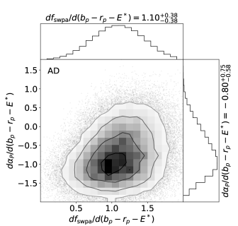
For our model where (instead of ) is a linear function of , we find a negative slope for the linear relation between and color: using KS distances (similarly using AD). The period power–law index at the median color is . In Figure 4 (bottom panel), we also plot the best–fitting (KS) relations for as a function of . Similar to the middle panel, the bold red line shows an example (with and ), while the thin red lines and shaded region show 100 models each passing our KS distance threshold and the 68.3% region, respectively. For reference, corresponds to a flat distribution in log–period. Thus, we find that in this model, the occurrence of planets in our period range increases toward longer periods for nearly all FGK dwarfs, with a sharper rise for earlier type (bluer) stars and a shallower rise for later type stars. Since planets at shorter periods are more likely to transit and are easier to detect than planets at longer periods, this would imply that the observed rise in planet occurrence toward later spectral types can be explained by there being more short period planets for redder stars than for bluer stars. However, this relation is tentative at best, and we caution against using this model for reasons described below.
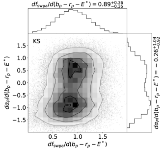
While the linear model provides overall best–fitting distances to the Kepler planet catalog similar to the linear model (Appendix Figures A4 and A5), a more detailed analysis shows that the linear relation between and color is questionable. Compared to the model, the negative slope for improves the fit to the period distribution of the bluer planet sample, but worsens the fit to the transit duration distribution of the same half. Most importantly, the value of is not robustly determined when simultaneously including both the linear and linear functions of in our model. In Figure 6, we plot the joint posterior distributions of and for such a model. We find that () using KS (AD) analyses, results that are significantly closer to zero than in the model where only is allowed to vary with color. The distribution using KS distances appears slightly bimodal, with one mode above and one below zero, although the nature is unknown and this is not seen in the AD results; in either case, is consistent with no slope. In contrast, the slope for with color is just as strong as in our linear model and still significantly positive: () using KS (AD) analyses. Taken together, our results show that while varying or with color can have similar effects on the rate of observed planets as a function of stellar type (as we will further show in §4.1), a change in is the more likely explanation. We conclude that the linear model is the preferred model, with the fraction of stars with planets clearly increasing toward later spectral types, as has been previously shown.
| Kepler data | Constant | Linear | Linear | |||||||||
|---|---|---|---|---|---|---|---|---|---|---|---|---|
| All | Bluer | Redder | All | Bluer | Redder | All | Bluer | Redder | All | Bluer | Redder | |
| 1 | 1218 | 554 | 664 | |||||||||
| 2 | 261 | 120 | 141 | |||||||||
| 3 | 101 | 38 | 63 | |||||||||
| 4 | 30 | 12 | 18 | |||||||||
| 5 | 7 | 4 | 3 | |||||||||
| 6 | 3 | 1 | 2 | |||||||||
| 7 | 0 | 0 | 0 | |||||||||
| 8 | 0 | 0 | 0 | |||||||||
| Totals | 2216 | 982 | 1234 | |||||||||
Note. — The “Bluer” and “Redder” columns add up to the “All” columns. For each model, the 68.3% credible intervals are computed from 1000 simulated catalogs passing the (KS) distance threshold (the results from our AD analyses, not shown, are similar but yield somewhat larger uncertainties). While all three models fit the overall (“All”) multiplicity distribution equally well (and produce nearly identical distributions), the linear models produce much better matches to the observed multiplicities of both the bluer and redder halves. We plot ratios of the model columns to the Kepler columns in Figure 7.
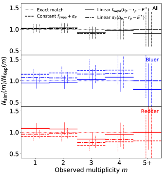
While all three models fit the overall multiplicity distribution equally well (top panel), the constant model significantly overproduces observed systems around the bluer stars and underproduces systems around the redder stars in our sample. Our linear models are a better fit to the observed multiplicities for these two subsets, with the linear model providing the best fits.
4 Discussion
4.1 The Observed Multiplicity Distribution
In Table 4, we list the observed multiplicity counts from the Kepler planet catalog and our models (constant , linear , and linear ), in the total (“All”) sample as well as in the bluer and redder halves. For the multiplicity counts observed from our models, we also compute and list uncertainties from generating 1000 simulated catalogs that pass our (KS) distance threshold. The results using our AD distance threshold are similar for the median values but provide somewhat larger uncertainties (which we have not listed here). We note that the 68.3% credible regions we computed include two sources of uncertainty: (1) the Monte Carlo noise due to the finite number of targets used for each simulated catalog (which we set to be equal to the number of targets in our Kepler stellar sample, 88,912 stars), and (2) the differences in the models due to the uncertainties in the model parameters, for which we only keep sets of parameters passing the distance threshold after one realization of a simulated catalog.
To facilitate a more direct comparison between the multiplicity distributions observed in the Kepler catalog and our models, we also plot the ratios of our models to the Kepler counts, , for each observed planet multiplicity order in Figure 7. We show panels for the total, bluer, and redder samples, computing the ratios of observed model counts to Kepler counts for each sample. In each panel, horizontal bars denote the median ratio values (an exact match is given by a ratio of 1, guided by the dotted line), while vertical lines show the 68.3% credible intervals (as listed in Table 4). The dashed, solid, and dash–dotted lines plot the results from our constant , linear , and linear models, respectively. Systems with observed planets are binned together here because of their low counts (the same multiplicity binning is also done in our distance function when computing in equation 4).
The models explored in this paper fit the overall multiplicity distribution equally well. This is expected, as Paper I showed that a clustered model (with two populations of mutual inclinations) is necessary and fits the observed multiplicity distribution extremely well; the models in this paper are extensions of that model. For almost all multiplicity orders , the median observed counts from our models very closely match the Kepler count, and the latter falls within our 68.3% credible intervals. The biggest difference is the number of triples (), as more triple systems are observed in the data (101, given our period–radius range and stellar sample) than what our models produce. However, the number is still within the 68.3% credible intervals (, , and for our constant , linear , and linear models, respectively).
The need for a stellar–dependent (or ) is clear when considering the bluer and redder halves of our FGK dwarf sample. Our baseline (constant ) model consistently overproduces the rate of observed planetary systems around bluer stars and underproduces the rate around redder stars. This trend is significant at all observed multiplicity orders except the higher ones at and , where the relatively low counts reduce the statistical power to distinguish between the two models. On the other hand, each of our linear models provides a significantly better match to the observed multiplicity distributions around both the bluer and redder halves compared to the constant model. The decreasing relation of with color can appear to account for the observed rates of planets as a function of spectral type, in a similar manner as increasing the . However, the linear model (solid lines) appears to provide an overall slightly closer match than the linear model (dash–dotted lines). Interestingly, while the number of observed triples is a near exact match in the bluer sample, there is a higher occurrence of triples in the redder sample than what our model produces. Nevertheless, the excellent similarity between the multiplicity distributions of this model and the Kepler data for both the bluer and redder halves is remarkable, given that our model assumes a very simple stellar dependence, the fraction of stars with planets as a simple linear function of the Gaia color, and that we have not made any other parameters of the model depend on the stellar properties.
4.2 Why Does Our Constant Model Produce More Detected Planets Around Hotter Stars?
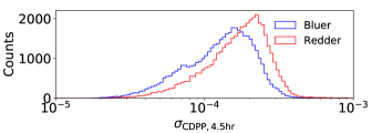
As we show in Table 4, splitting our Kepler sample of stars into two equal–sized halves based on their Gaia colors includes more observed planets around redder stars than around bluer stars, at almost all multiplicity orders (except , although the total counts at high are small). On first glance, it is unclear if the higher rate of observed planets around redder stars is due to an observational bias in favor of smaller, cooler stars, or an inherent increase in the underlying planet occurrence rate, or some combination of both. However, in this paper we showed with our forward model that we get a modestly higher overall rate of observed planets around stars in the bluer half than in the redder half if we assume the same distribution of planetary systems (i.e. our baseline, constant model): versus planets in total for the bluer and redder samples, respectively. Indeed, the tension between these counts and that of the Kepler data is why we require a dependence on the stellar color/effective temperature in order to produce the number of observed planets in both stellar samples. So why is it seemingly easier to detect planets of a given size and period around hotter stars?
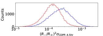
On one hand, the larger sizes of bluer (hotter) stars provide one clear disadvantage for detecting transiting planets of a given size, since to first order the transit depth is given by the fraction of the stellar disk area blocked by the planet, ; that is, it is inversely proportional to the stellar radius squared. On the other hand, planets are more likely to transit larger stars simply due to the increased geometric transit probability (). Larger stars may also induce longer transit durations, due to the distance a planet must travel in order to cross the stellar disk ( to first order). Another factor contributing to the increased detection efficiency of planets around bluer stars in the Kepler mission is their improved photometric precision over that of redder stars, due to their brightness.
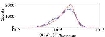
To illustrate how each of these factors affect the relative detectability of planets around bluer versus redder stars in our FGK sample, we show a sequence of histograms of relevant quantities involving stellar radius and the root mean square Combined Differential Photometric Precision (Christiansen et al., 2012), (4.5 hr duration for simplicity), for our bluer and redder stellar samples in Figure 8 (including all stars, not just known planet hosts, in our sample). The distribution of for the bluer stars is shifted toward lower values than that of the redder stars, making it easier to detect transits of a given depth (top panel). Including the dependence on stellar radii of the transit depth, we have , a “single–measurement signal–to–noise ratio (S/N)”. This distribution (middle panel) shows that for a transiting planet with fixed size and transit duration, the decrease in transit depth is typically greater than the improvement in , thus favoring detections around redder stars. Factoring in the transit duration to the S/N () and the geometric transit probability () gives a “transit geometry–weighted S/N” that is proportional to (bottom panel). While the distributions of the bluer and redder samples are quite similar, the lower tail of the distribution () includes more bluer stars. This means that the rate of detections for the smallest detectable planets is enhanced for the bluer stars in our sample. Finally, since the occurrence of planets increases toward smaller sizes (e.g., we find for the power–law index of small planets for the models presented in this paper), the smallest detectable planets contribute most to the overall rate of observed planets. This confirms our finding with the full model that if the fraction of stars with planets were independent of stellar color, that we would find somewhat more planets around bluer stars than redder stars (as in Table 4).
4.3 Are Orbital Eccentricities Correlated with Stellar Type?
In order to briefly explore correlations between stellar type and other parameters in our model, we also test a model in which the eccentricity scale is allowed to vary as a function of . For this analysis, we use the same procedure as described in §2, except we adopt the circular–normalized transit duration () in place of the transit duration () when computing the distance. The distribution of is more sensitive to the intrinsic eccentricity distribution, but requires the stellar properties (e.g. mean density) to be very well characterized (e.g., Moorhead et al., 2011; Plavchan, Bilinski, & Currie, 2014; Van Eylen & Albrecht, 2015; Xie et al., 2016). While we adopt stellar radii from Gaia DR2, the stellar masses remain from Kepler DR25; for this reason, we have avoided using in the analyses for all the other models. Nevertheless, we perform a cursory analysis to see if there are any clear trends between eccentricity and spectral type.
For simplicity, we also assume a linear relation parameterized by a slope and -intercept (at median color, ; analogous to the form of equation 1). We allow for to vary in and in . We find no clear trend between and in this analysis; while is constrained to similarly low values of , the slope takes on both positive and negative values. Interestingly, there appears to be a slight preference for positive or negative slopes compared to zero slope. We interpret this as suggesting that there is evidence for a higher-eccentricity population of exoplanets, but that this is not dependent on the host star color.
 |
 |
 |
 |
 |
 |
4.4 Other Correlations in Planetary System Architectures with Stellar Type
The models presented in Paper I and in this paper are driven by fits to the marginal distributions of a collection of key observables for the Kepler DR25 catalog of exoplanet candidates, as listed in §2.2.1. As discussed in §2.2, this study adopted a distance function that incorporates simultaneous fits to these summary statistics in the total, bluer, and redder samples in order to infer the best-fitting model parameters. While we did not explicitly explore how the planetary system properties vary with color for all of our other architectural model parameters, we can examine fits to the observed data for our linear (and linear ) models in order to discern possible differences in the architectures between the two samples. We note that we also attempted to fit the constant model to each of the bluer and redder samples, independently, but found that we could not adequately constrain all of the model parameters, including the differences in . This is perhaps unsurprising, due to the reduced inference power of using half the data (or another way to think about it is that there are twice as many free parameters to describe the same data). Nevertheless, in this analysis we did not find any evidence for clear differences in the other parameters (i.e. the mean rates of clusters and planets per cluster, eccentricity and mutual inclination scales, and clustering scales in periods and radii) between the bluer and redder halves, suggesting that planetary system architectures are quite similar across all main sequence FGK spectral types.
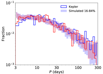
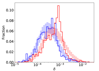
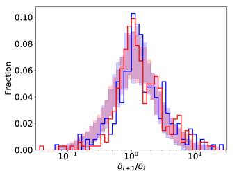
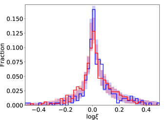
We plot the marginal distributions of observed properties from our catalogs using our best–fitting linear model in Figure 9 (with the parameters listed in Table 3), where the model and the Kepler data are split into the bluer and redder halves. A similar plot for the observed catalogs from our linear model is provided in Appendix Figure A3. The panels from left to right and top to bottom show the observed distributions of orbital periods (), period ratios (), transit depths (), transit depth ratios (), transit durations (), and period-normalized transit duration ratios (). In each panel, the shaded regions denote the central 68.3% credible interval (in each histogram bin) from 100 simulated catalogs passing the (KS) distance threshold, while the solid line histograms show the Kepler population given our sample. Figures A4 and A5 in the Appendix show how simulated catalogs passing the distance thresholds for KS and AD, respectively, compare to the Kepler catalog in terms of the individual (weighted) distance terms.
Overall, our linear model provides an excellent fit to the marginal distributions of the observed Kepler planet candidates, for both the bluer and redder samples as well as the combined sample. The best distances are as low as in both the bluer and redder samples and for the total sample; for comparison, a “perfect” model would result in for each of these samples given our number of distance terms. While many of the marginal distributions are fit nearly perfectly (i.e. have individual weighted distances around unity, given Monte Carlo noise), there are some differences between the Kepler data and our model predictions, both subtle and significant (e.g. the transit depth and depth ratio distributions). The bulk of the period distribution is well modeled, although there is a deviation at short periods suggesting a need for a more complicated model than the single power-law we have adopted (e.g., Howard et al. 2012; Mulders, Pascucci, & Apai 2015; Mulders et al. 2018). There are fewer planets at the shortest orbital periods we investigated ( d) around the bluer stars than around the redder stars (note the log -scale) and the fit to the period distribution is worse, suggesting that the inner edge of planetary systems may be stellar dependent as also found by Plavchan, Bilinski, & Currie (2014) and Mulders, Pascucci, & Apai (2015). Indeed, this is likely driving the results of our linear model; the period distribution is a slightly better fit for this model compared to the linear model, although only for the bluer sample. The fit to the period ratios is nearly identical for both linear models.
The transit depth distribution is very different between our two stellar samples as expected because of the different distributions of stellar radii and photometric precision, but the fit to the redder half is clearly worse than that of the bluer half, due to an apparent excess of transit depths at in the data. On the other hand, the transit depth ratio distribution is very similar between the two stellar samples (in both the data and our models). As in Paper I, we note that while our simple clustering in planet sizes is necessary to explain the highly peaked nature of the distribution, it is not sufficient to explain the asymmetry caused by larger planets being more often the outer planet in observed adjacent pairs (Ciardi et al. 2013; Weiss et al. 2018a; Gilbert & Fabrycky 2020). The intrinsic planet radius distribution is sculpted by the processes of photoevaporation (Owen & Wu, 2013; Fulton et al., 2017; Owen & Wu, 2017; Van Eylen et al., 2017; Carrera et al., 2018) and/or heating from formation (e.g. core-powered mass-loss; Ginzburg, Schlichting, & Sari 2016, 2018; Gupta & Schlichting 2018), which our broken power-law with clustering for planet sizes cannot fully encapsulate.
The transit duration distributions differ between the bluer and redder halves as expected due to the dependencies on stellar radius and density. There are some tradeoffs in the fits to the distributions for each half between the models. While the linear model improves the fits to both samples compared to the constant model, it is intriguing that the linear model provides the best fit to the redder distribution and the worst fit to the bluer distribution (even compared to the constant model), which is a reversal to the period distribution fits. In any case, the linear model significantly improves the fit to the overall distribution over the constant or linear models. This is easily explained by the overall better matches to the frequency of observed planets of the bluer and redder halves in our linear model. The constant model provides too many planets around the bluer stars, which have a different distribution than that of the planets around the redder stars, while the linear model provides just the right contributions. Finally, we see no difference in the fits to the period-normalized transit duration ratio distributions, which are modeled extremely well.
5 Conclusions
We have extended our forward modeling methodology from He, Ford, & Ragozzine (2019) (Paper I) to explore how the occurrence of planetary systems and their architectures may vary as a function of their host stars, using the Gaia DR2 colors as a proxy for stellar effective temperature (i.e. spectral type). We use a clean sample of 88,912 Kepler FGK dwarfs (a stellar catalog similar to the one defined in Hsu et al. 2019, but with an additional reddening correction) and the Kepler DR25 candidates with periods of days and radii of (the same range as explored in Paper I), and we define to refer to the fraction of stars that host at least one planet in this range.
First, we adopt the clustered periods and sizes model from Paper I and re-parameterize the intrinsic multiplicity distribution by decoupling the fraction of stars with planets () from the number of clusters and planets per cluster, to form our baseline (constant ) model. We show that this does not change our main results about the architectures of planetary systems, namely the underlying power-laws for the period and radius distributions, the extent of intra-cluster similarity in periods and planet radii, the role of two populations of multi-planet systems with different mutual inclination scales in order to explain the observed Kepler dichotomy, and the overall marginalized over all FGK stars.
Then, we generalize our baseline clustered model to test linear dependencies on stellar color for several model parameters, including the fraction of stars with planets (), the period power–law index (), and the eccentricity scale (). We use the Gaia DR2 colors as a proxy for spectral type and correct for differential reddening using a simple model for . By splitting our stellar sample of FGK stars into two halves (bluer and redder) based on their colors, modifying our distance function to fit to the observed marginal distributions of both halves and the overall sample, and performing model inference using ABC, we find the following results:
-
•
For our stellar and planet sample, dividing the stars into two equal–sized halves at the median color results in more Kepler planets being observed around redder stars than around bluer stars. The relative counts are shaped by a combination of observational biases (arising from differing stellar properties, photometric precision, and so on) and intrinsic planet occurrence rates.
-
•
The smallest sized planets are easier to detect around earlier type (hotter and bluer) stars in the Kepler mission. While redder stars are smaller in size and thus induce larger transit depths for a given size of planet, bluer stars benefit from causing increased transit durations, geometric transit probability, and better photometric precision. Our forward model accounts for all of these effects. Assuming a constant rate of planetary systems across all stars (i.e., our constant model) produces more detected planets in the bluer sample and fewer in the redder sample, significantly at odds with the Kepler counts.
-
•
The two points above imply that the overall occurrence of planets increases toward later type dwarfs (cooler and redder stars), in agreement with the general trends reported in Howard et al. (2012) and Mulders, Pascucci, & Apai (2015). We find that this increase in planet occurrence is well described by a change in the fraction of stars with planets (), similar to the findings of Yang, Xie, & Zhou (2020). Assuming a linear trend with color, we find a significant positive slope of () using KS (AD) analyses. This implies that there is a substantial difference in the fraction of stars hosting planetary systems across FGK stars: for F2V dwarfs and for mid K dwarfs. The solar value is roughly half: for G2V. While our linear relation is likely an oversimplification at the extreme ends of our sample, extrapolating to later type stars suggests that planetary systems are ubiquitous around early M-dwarfs, as has been shown previously by Ballard & Johnson (2016). Note that this is in addition to the high rate of planets per M-dwarf star, as suggested by Dressing & Charbonneau (2013); Mulders, Pascucci, & Apai (2015); Hardegree-Ullman et al. (2019).
-
•
We verify that the increase in toward later type stars is robust by exploring a step function in which the fraction of stars with planets is a constant below and above the median color. In this step model, we find a significant difference, with () using KS (AD) analyses. The higher for redder stars is fully consistent with the results of our linear parameterization.
-
•
We test an alternative explanation for the increased planet occurrence toward later types, by considering a change in the period power–law distribution, with a shallower rise in occurrence toward longer periods for planets around redder stars compared to bluer stars (characterized by a negative where is the power–law index). We find that this trend is only necessary when we hold fixed with color, but disappears when simultaneously allowing for linear functions of for both and . In either case, the strong positive slope of remains, strengthening the results of our linear model.
-
•
While both linear and models improve the fits to the observed planet multiplicity distributions of our bluer and redder samples over the constant model, the linear model provides the best fit.
-
•
The other architectural model parameters do not change significantly when including the stellar dependencies in our clustered model. Our constant , linear , and linear models result in similar rates of clusters and planets, radius distributions, eccentricity scales, and evidence for two populations of mutual inclinations.
-
•
We find no clear correlation between orbital eccentricity and spectral type, although there may be some evidence for a population of planets with more highly eccentric orbits than our single Rayleigh distribution with .
Our findings have consequences for informing future follow-up observations of exoplanet detections from the Transiting Exoplanet Survey Satellite (TESS) mission, which has completed its two-year primary mission (Ricker et al., 2015; Sullivan et al., 2015; Stassun et al., 2018) and is poised for extended missions (Bouma et al., 2017; Huang et al., 2018). With already over 1000 planet candidates collected, the TESS mission is expected to discover many more short-period ( d) planets around nearby stars that are most amenable to RV follow-up (Barclay, Pepper, & Quintana, 2018; Stassun et al., 2018). Being a magnitude limited survey, the TESS mission will observe many more brighter targets (e.g. F stars, compared to later types) in its full field images. Our results show that while these nearby bright stars may be more tenable for transit recovery, the intrinsic rate of inner planetary systems is relatively low for these bluer stars and increases significantly toward later type stars. Thus, follow-up efforts should also target these fainter stars as multi-planet systems around such hosts are common (Ballard & Johnson, 2016; Ballard, 2019). In any case, the primary and extended missions of TESS will likely boost our catalogs of planet candidates around a wide variety of stellar types, further enabling new studies on the architectures of planetary systems as a function of host star properties.
Additional planet companions in systems with short period transiting planets discovered by TESS can also provide stronger constraints on the mutual inclination distribution of multi-planet systems. This may allow future studies to differentiate between a dichotomous model, such as the one considered in this study, and other competing models (Zhu et al., 2018; Zink, Christiansen, & Hansen, 2019).
The new catalogs generated from our models are available to the public, along with the core SysSim code (https://github.com/ExoJulia/ExoplanetsSysSim.jl), inputs collated from numerous data files (https://github.com/ExoJulia/SysSimData), and the code specific to the clustered models (https://github.com/ExoJulia/SysSimExClusters). We encourage other researchers to contribute model extensions via Github pull requests and/or additional public git repositories.
References
- Anderson & Darling (1952) Anderson, T. W. & Darling, D. A. 1952, The Annals of Mathematical Statistics, 23, 193
- Andrae et al. (2018) Andrae, R., Fouesneau, M., Creevey, O., et al. 2018, A&A, 616, A8
- Bailer-Jones et al. (2018) Bailer-Jones, C. A. L., Rybizki, J., Fouesneau, M., et al. 2018, AJ, 156, 58
- Ballard (2019) Ballard, S. 2019, AJ, 157, 113
- Ballard & Johnson (2016) Ballard, S. & Johnson, J. A. 2016, ApJ, 816, 66
- Barclay, Pepper, & Quintana (2018) Barclay, T., Pepper, J., & Quintana, E. V. 2018, ApJS, 239, 2
- Batalha et al. (2013) Batalha, N. M., Rowe, J. F., Bryson, S. T., et al. 2013, ApJS, 204, 24
- Berger et al. (2020) Berger, T. A., Huber, D., van Saders, J. L., et al. 2020, AJ, 159, 280
- Bonfils et al. (2013) Bonfils, X., Delfosse, X., Udry, S., et al. 2013, A&A, 549, A109
- Borucki et al. (2010) Borucki, W. J., Koch, D. G., Basri, G., et al. 2010, Science, 327, 977
- Borucki et al. (2011a) Borucki, W. J., Koch, D. G., Basri, G., et al. 2011a, ApJ, 728, 117
- Borucki et al. (2011b) Borucki, W. J., Koch, D. G., Basri, G., et al. 2011b, ApJ, 736, 19
- Bouma et al. (2017) Bouma, L. G., Winn, J. N., Kosiarek, J., & McCullough, P. R. 2017, arXiv:1705.08891
- Bryson (2020) Bryson, S. 2020 Res. Notes AAS, 4, 32
- Burke & Catanzarite (2017a) Burke, C. J., & Catanzarite, J. 2017a, Planet Detection Metrics: Window and One-Sigma Depth Functions for Data Release 25, Tech. Rep. KSCI-19101-002
- Burke & Catanzarite (2017b) Burke, C. J., & Catanzarite, J. 2017b, Planet Detection Metrics: Per-Target Flux-Level Transit Injection Tests of TPS for Data Release 25, Tech. Rep. KSCI-19109-002
- Burke & Catanzarite (2017c) Burke, C. J., & Catanzarite, J. 2017c, Planet Detection Metrics: Per-Target Detection Contours for Data Release 25, Tech. Rep. KSCI-19111-002
- Carrera et al. (2018) Carrera, D., Ford, E. B., Izidoro, A., et al. 2018, ApJ, 866, 104
- Catanzarite & Shao (2011) Catanzarite, J. & Shao, M. 2011, ApJ, 738, 151
- Christiansen et al. (2012) Christiansen, J. L., Jenkins, J. M., Caldwell, D. A., et al. 2012, PASP, 124, 1279
- Christiansen et al. (2020) Christiansen, J. L., Clarke, B. D., Burke, C. J., et al. 2020, AJ, 160, 159
- Ciardi et al. (2013) Ciardi, D. R., Fabrycky, D. C., Ford, E. B., et al. 2013, ApJ, 763, 41
- Coughlin (2017) Coughlin, J. L. 2017, Planet Detection Metrics: Robovetter Completeness and Effectiveness for Data Release 25, Tech. Rep. KSCI-19114-001
- Cressie & Read (1984) Cressie, N. & Read, T. R. C. 1984, Journal of the Royal Statistical Society. Series B, 46, 440
- Cumming et al. (2008) Cumming, A., Butler, R. P., Marcy, G. W., et al. 2008, PASP, 120, 531
- Dressing & Charbonneau (2013) Dressing, C. D. & Charbonneau, D. 2013, ApJ, 767, 95
- Endl et al. (2006) Endl, M., Cochran, W. D., Kürster, M., et al. 2006, ApJ, 649, 436
- Fabrycky et al. (2014) Fabrycky, D. C., Lissauer, J. J., Ragozzine, D., et al. 2014, ApJ, 790, 146
- Fang & Margot (2012) Fang, J., & Margot, J.-L. 2012, ApJ, 761, 92
- Ford et al. (2018b) Ford, E. B., He, M. Y., Hsu, D. C., & Ragozzine, D. 2018b, Planetary Systems Simulation & Model of Kepler Mission for Characterizing the Occurrence Rates of Exoplanets and Planetary Architectures, v1.0, Zenodo, doi:10.5281/zenodo.1205172. https://doi.org/10.5281/zenodo.1205172
- Ford (2019) Ford, E. B., 2019, ExoJulia/SysSimData: Initial Release of Data Files for the Exoplanet System Simulator, v1.0.0 Zenodo, doi:10.5281/zenodo.3255313. https://doi.org/10.5281/zenodo.3255313
- Foreman-Mackey (2016) Foreman-Mackey, D. 2016, corner.py: Scatterplot matrices in Python, JOSS, 1, 24, doi:10.21105/joss.00024
- Fressin et al. (2013) Fressin, F., Torres, G., Charbonneau, D., et al. 2013, ApJ, 766, 81
- Fulton et al. (2017) Fulton, B. J., Petigura, E. A., Howard, A. W., et al. 2017, AJ, 154, 109
- Gaia Collaboration et al. (2018) Gaia Collaboration, Brown, A. G. A., Vallenari, A., et al. 2018, A&A, 616, A1
- Gaidos et al. (2013) Gaidos, E., Fischer, D. A., Mann, A. W., et al. 2013, ApJ, 771, 18
- Gaidos et al. (2016) Gaidos, E., Mann, A. W., Kraus, A. L., et al. 2016, MNRAS, 457, 2877
- Gilbert & Fabrycky (2020) Gilbert, G. & Fabrycky, D. 2020, AJ, 159, 281
- Ginzburg, Schlichting, & Sari (2016) Ginzburg, S., Schlichting, H. E., & Sari, R. 2016, ApJ, 825, 29
- Ginzburg, Schlichting, & Sari (2018) Ginzburg, S., Schlichting, H. E., & Sari, R. 2016, MNRAS, 476, 759
- Gupta & Schlichting (2018) Gupta, A. & Schlichting, H. E. 2018, MNRAS, 487, 24
- Hardegree-Ullman et al. (2019) Hardegree-Ullman, K. K., Cushing, M. C., Muirhead, P. S., & Christiansen, J. L. 2019, AJ, 158, 75
- He, Ford, & Ragozzine (2019) He, M. Y., Ford, E. B., & Ragozzine, D. 2019, MNRAS, 490, 4575
- Howard et al. (2012) Howard, A. W., Marcy, G. W., Bryson, S. T., et al. 2012, ApJS, 201, 15
- Hsu et al. (2018) Hsu, D. C., Ford, E. B., Ragozzine, D., et al. 2018, AJ, 155, 205
- Hsu et al. (2019) Hsu, D. C., Ford, E. B., Ragozzine, D., & Ashby, K. 2019, AJ, 158, 109
- Hsu, Ford, & Terrien (2020) Hsu, D. C., Ford, E. B., & Terrien, R. 2020, MNRAS, 498, 2249
- Huang et al. (2018) Huang, C. X., Shporer, A., Dragomir, D., et al. 2018, Expected Yields of Planet discoveries from the TESS primary and extended missions, arXiv:1807.11129
- Hunter (2007) Hunter, J. D. 2007, Computing in Science and Engineering, 9, 90
- Johnson et al. (2018) Johnson, J. A., Petigura, E. A., Fulton, B. J., et al. 2017, AJ, 154, 108
- Kolmogorov (1933) Kolmogorov, A. N. 1933, Giornale dell’Istituto Italiano degli Attuari, 4, 83
- Lannier et al. (2016) Lannier, J., Delorme, P., Lagrange, A. M., et al. 2016, A&A, 596, A83
- Latham et al. (2011) Latham, D. W., Rowe, J. F., Quinn, S. N., et al. 2011, ApJL, 732, L24
- Lissauer et al. (2011a) Lissauer, J. J., Fabrycky, D. C., Ford, E. B., et al. 2011a, Nature, 470, 53
- Lissauer et al. (2011b) Lissauer, J. J., Ragozzine, D., Fabrycky, D. C., et al. 2011b, ApJS, 197, 8
- Lissauer et al. (2014) Lissauer, J. J., Marcy, G. W., Bryson, S. T., et al. 2014, ApJ, 784, 44
- Moorhead et al. (2011) Moorhead, A. V., Ford, E. B., Morehead, R. C., et al. 2011, ApJS, 197, 1
- Mulders, Pascucci, & Apai (2015) Mulders, G., Pascucci, I., & Apai, D. 2015, ApJ, 798, 112
- Mulders et al. (2018) Mulders, G. D., Pascucci, I., Apai, D., et al. 2018, AJ, 156, 24
- Ning, Wolfgang, & Ghosh (2018) Ning, B., Wolfgang, A., & Ghosh, S. 2018, ApJ, 869, 5
- Owen & Wu (2013) Owen, J. E. & Wu, Y. 2013, Kepler Planets: A Tale of Evaporation, ApJ, 775, 105
- Owen & Wu (2017) Owen, J. E. & Wu, Y. 2017, ApJ, 847, 29
- Pecaut & Mamajek (2013) Pecaut, M. J. & Mamajek, E. E. 2013, ApJS, 208, 9
- Petigura, Marcy, & Howard (2013b) Petigura, E. A., Marcy, G. W., & Howard, A. W. 2013b, ApJ, 770, 69
- Pettitt (1976) Pettitt, A. N. 1976, Biometrika, 63, 161
- Plavchan, Bilinski, & Currie (2014) Plavchan, P., Bilinski, C., & Currie, T. 2014, PASP, 126, 935
- Ragozzine & Holman (2010) Ragozzine, D. & Holman, M. J. 2010, arXiv:1006.3727
- Rasmussen & Williams (2006) Rasmussen, C. E. & Williams, C. K. I. 2006, Gaussian Processes for Machine Learning, MIT Press, ISBN 0-262-18253-X
- Ricker et al. (2015) Ricker, G. R., Winn, J. N., Vanderspek, R., et al. 2015, JATIS, 1, 014003
- Rowe et al. (2014) Rowe, J. F., Bryson, S. T., Marcy, G. W., et al. 2014, ApJ, 784, 45
- Rowe et al. (2015) Rowe, J. F., Coughlin, J. L., Antoci, V., et al. 2015, ApJS, 217, 16
- Sandford, Kipping, & Collins (2019) Sandford, E., Kipping, D., & Collins, M. 2019, MNRAS, 489, 3162
- Smirnov (1948) Smirnov, N. 1948, The Annals of Mathematical Statistics, 19, 279
- Stassun et al. (2018) Stassun, K. G., Oelkers, R. J., Pepper, J., et al. 2018, AJ, 156, 102
- Steffen et al. (2010) Steffen, J. H., Batalha, N. M., Borucki, W., J., et al. 2010, ApJ, 725, 1226
- Sullivan et al. (2015) Sullivan, P. W., Winn, J. N., Berta-Thompson, Z. K., et al. 2015, ApJ, 809, 77
- Thompson et al. (2018) Thompson, S. E., Coughlin, J. L., Hoffman, K., et al. 2018, ApJS, 235, 38
- van der Walt et al. (2011) van der Walt, S., Colbert, S. C., & Varoquaux, G. 2011, CSE, 13, 22
- Van Eylen & Albrecht (2015) Van Eylen, V. & Albrecht, S. 2015, ApJ, 808, 126
- Van Eylen et al. (2017) Van Eylen, V., Agentoft, C., Lundkvist, M. S., et al. 2018, MNRAS, 479, 4786
- Weiss et al. (2018a) Weiss, L. M., Marcy, G. W., Petigura, E. A., et al. 2018, AJ, 155, 48
- Winn & Fabrycky (2015) Winn, J. N. & Fabrycky, D. C. 2015, ARA&A, 53, 407
- Xie et al. (2016) Xie, J.-W., Subo, D., Zhu, Z., et al. 2016, PNAS, 113, 11431
- Yang, Xie, & Zhou (2020) Yang, J.-Y., Xie, J.-W., & Zhou, J.-L. 2020, AJ, 159, 164
- Zhu et al. (2018) Zhu, W., Petrovich, C., Wu, Y., et al. 2018, ApJ, 860, 101
- Zink, Christiansen, & Hansen (2019) Zink, J. K., Christiansen, J. L., & Hansen, B. M. S. 2019, MNRAS, 483, 4479
- Zink & Hansen (2019) Zink, J. K. & Hansen, B. M. S. 2019, MNRAS, 487, 246
Figures A1 and A2 show the ABC posterior distributions for the model parameters of our constant and linear models, respectively. In Figure A3, we show the observed marginal distributions of our linear model, for comparison with the linear model in Figure 9. While the observed distributions appear very similar between the two models, there are subtle differences in how they fit the marginal distributions of the Kepler planet candidates. These differences are more clearly seen in Figures A4 and A5, where we show how a large number of simulated catalogs from each of the three primary models considered in this study compare to the Kepler catalog in terms of the individual (weighted; KS and AD) distance terms for each observable distribution.
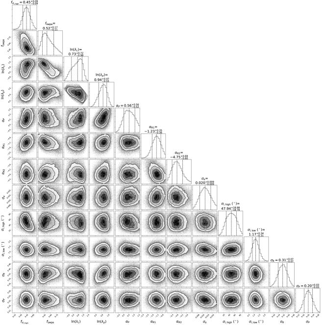
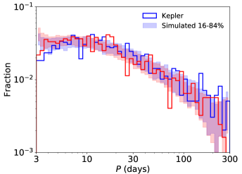 |
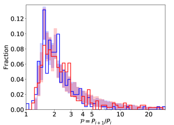 |
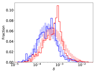 |
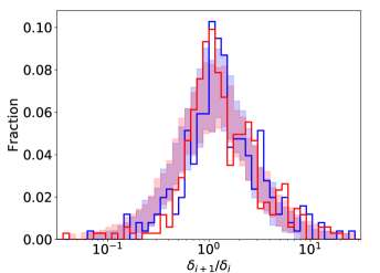 |
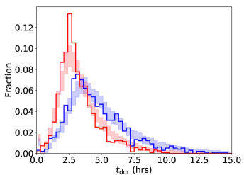 |
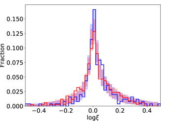 |
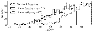 |
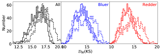 |
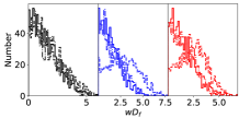 |
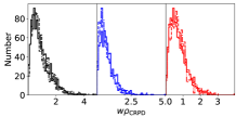 |
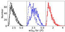 |
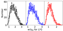 |
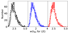 |
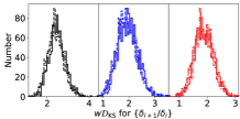 |
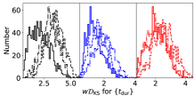 |
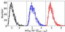 |
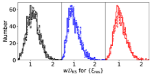 |
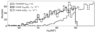 |
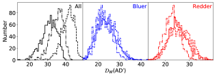 |
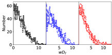 |
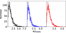 |
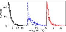 |
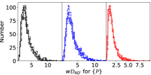 |
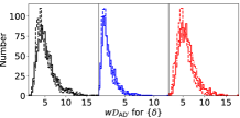 |
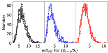 |
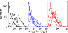 |
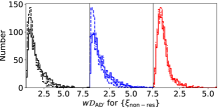 |
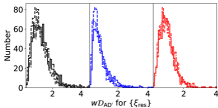 |