Magnetic Reconnection and Hot Spot Formation in Black Hole Accretion Disks

Abstract

Hot spots, or plasmoids, forming due to magnetic reconnection in current sheets, are conjectured to power frequent X-ray and near-infrared flares from Sgr A^∗, the black hole in the center of our Galaxy. It is unclear how, where, and when current sheets form in black-hole accretion disks. We perform axisymmetric general-relativistic resistive magnetohydrodynamics simulations to model reconnection and plasmoid formation in a range of accretion flows. Current sheets and plasmoids are ubiquitous features which form regardless of the initial magnetic field in the disk, the magnetization in the quasi-steady-state phase of accretion, and the spin of the black hole. Within 10 Schwarzschild radii from the event horizon, we observe plasmoids forming, after which they can merge, grow to macroscopic scales of the order of a few Schwarzschild radii, and are ultimately advected along the jet’s sheath or into the disk. Large plasmoids are energized to relativistic temperatures via reconnection and contribute to the jet’s limb-brightening. We find that only hot spots forming in magnetically arrested disks can potentially explain the energetics of Sgr A^∗ flares. The flare period is determined by the reconnection rate, which we find to be between $0.01c$ and $0.03c$ in all cases, consistent with studies of reconnection in isolated Harris-type current sheets. We quantify magnetic dissipation and non-ideal electric fields which can efficiently inject non-thermal particles. We show that explicit resistivity allows for converged numerical solutions, such that the electromagnetic energy evolution and dissipation become independent of the grid scale for the extreme resolutions considered here.

1 Introduction

Bright, coincident episodic X-ray and near-infrared flares are detected on roughly a daily basis coming from Sgr A^∗, the supermassive black hole in the center of our Galaxy (see e.g., Baganoff et al. 2001; Genzel et al. 2003; Marrone et al. 2008; Meyer et al. 2008; Neilsen et al. 2013; Fazio et al. 2018; Boyce et al. 2019). The origin of these flares is generally associated with electron acceleration in a localized flaring region not larger than a few gravitational radii rather than with a global increase in the accretion rate or jet power (Markoff et al. 2001; Dodds-Eden et al. 2009; Ponti et al. 2017). The Gravity Collaboration et al. (2018) recently reported the detection of positional changes of such near-infrared flares originating from within 10 gravitational radii of the black hole. The observed variable emission is conjectured to arise from the motion of a compact “hot spot” orbiting within a dynamical time scale of the compact object.

Dissipation of magnetic energy through the process of magnetic reconnection in thin current layers is conjectured as the main mechanism producing the energetic electrons powering flares and hot spots (Yuan et al. 2004; Broderick & Loeb 2005; Goodman & Uzdensky 2008; Younsi & Wu 2015; Ball et al. 2016; Li et al. 2017; Gutiérrez et al. 2020). If such a reconnection layer becomes thin enough it can be liable to the tearing instability, break up, and produce chains of plasmoids (Loureiro et al. 2007) that interact, merge, grow, and are advected with the flow. From local studies of current sheets we know that magnetic reconnection can accelerate electrons in plasmoids to form non-thermal energy distributions (Sironi & Spitkovsky 2014; Guo et al. 2014; Werner et al. 2015; Rowan et al. 2017; Werner et al. 2018) potentially explaining the observed flaring emission. However, the formation of such reconnection layers in accretion flows has not yet been understood due to the lack of a model that captures both the dissipative microphysics and the global dynamics of the disk and jet. It is therefore essential to study reconnection in global simulations of accretion flows.

The global dynamics of black-hole accretion flows and jet formation is typically accurately modeled with ideal (i.e., infinitely conductive) general-relativistic magnetohydrodynamics (GRMHD) simulations (see e.g., Porth et al. 2019; White et al. 2019). While ideal GRMHD has provided significant insight in accretion flows, dissipation occurs at the grid scale and the frozen-in condition (Alfvén 1942) is broken purely due to numerical resistivity, such that it is not a reliable framework to study reconnection and plasmoid formation. Current sheet formation, magnetic reconnection, and plasmoid production in accretion disks have so far however only been investigated with ideal GRMHD simulations (Ball et al. 2018; Kadowaki et al. 2019; Nathanail et al. 2020). The plasma in accretion flows like that of Sgr A^∗ is effectively collisionless such that reconnection occurs because of kinetic effects (Parfrey et al. 2019) that break the frozen-in condition. For example, the divergence of the electron pressure tensor essentially plays the role of an effective resistivity (Bessho & Bhattacharjee 2005). In general-relativistic resistive magnetohydrodynamics (GRRMHD) an explicit finite resistivity $\eta$ acts as a proxy for kinetic effects, presenting the simplest model of magnetic reconnection and plasmoid formation (Loureiro & Uzdensky 2016) in turbulent black-hole accretion flows. For Lundquist numbers $S=v_{A}L/\eta\gtrsim 10^{4}$, where $v_{A}$ is the Alfvén speed and $L$ is the typical length of the current sheet, resistive reconnection becomes plasmoid-dominated and evolves independently of the resistivity $\eta$ at a universal rate of $\sim 0.01v_{A}$ (Bhattacharjee et al. 2009; Uzdensky et al. 2010). An explicit resistivity also allows for a converged evolution of electromagnetic energy density and for studying how it is dissipated through Ohmic heating. Additionally, the GRRMHD equations inherently provide information on the evolution of non-ideal electric field which can be responsible for particle acceleration, non-existent in ideal GRMHD.

With current state-of-the-art GRRMHD simulations it has been impossible to resolve fast small-scale reconnection dynamics accurately enough to determine whether plasmoids can form and grow in accretion flows (Vourellis et al. 2019; Tomei et al. 2020). Extreme resolutions are necessary to resolve current sheets that are thin enough to be liable to the plasmoid instability, while also capturing the global accretion flow dynamics. A combination of an implicit-explicit (IMEX) time-stepping scheme (Ripperda et al. 2019c) to capture fast reconnection dynamics, together with adaptive mesh refinement (AMR) capabilities of the Black Hole Accretion Code (BHAC, Porth et al. 2017; Olivares et al. 2019) to accurately resolve the smallest scales in the system allows us to study resistive reconnection and plasmoid formation in black-hole accretion disks for the very first time. We employ the GRRMHD module of BHAC to investigate whether a hot spot can form and grow nearby the event horizon. Additionally, we measure the reconnection rate and investigate whether the time and length scales on which magnetic reconnection occurs and plasmoids form in the accretion flow is in accordance with the variability of the multi-wavelength emission as observed for Sgr A^∗.

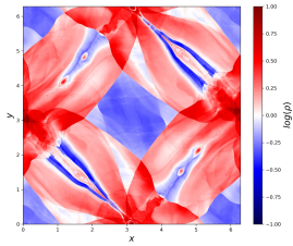
Figure 1: Rest-mass density $\rho$ for a vortex at $t=10t_{\rm c}$ for Lundquist number $S=10^{5}$. The plasmoids can be recognized as overdense blobs of plasma in the thin sheets.

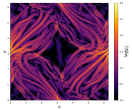
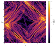
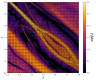
Figure 2: Logarithm of the out-of-plane current density magnitude $|J_{z}|$ at $t=10t_{\rm c}$ for $S=2\times 10^{3}$ (left), $S=2\times 10^{4}$ (middle), and a zoom into the current sheet for $S=2\times 10^{4}$ showing the AMR grid blocks (right), each consisting of $8\times 8$ cells, in black. Both cases have an effective resolution of $8192^{2}$ cells in the domain. The plasmoid-unstable current sheet on the right is captured by more than ten cells over its width.

A detailed outline of the numerical method used in this work, including a comprehensive description of the GRRMHD equations can be found in Ripperda et al. (2019c). From here onward we adopt Lorentz-Heaviside units where a factor of $1/\sqrt{4\pi}$ is absorbed into the electromagnetic fields and velocities are measured in units of the speed of light $c$. We employ a $3+1$ decomposition of the GRRMHD equations based on the Arnowitt-Deser-Misner formalism (Arnowitt et al. 1959) with a $(-,+,+,+)$ signature for the spacetime metric where Roman indices run over space only i.e., (1,2,3).

2 A toy model of relativistic turbulent reconnection

We study the properties of reconnection and formation of plasmoids in current sheets in an Orszag-Tang vortex (Orszag & Tang 1979) as a simplistic toy model for a turbulent flow. We also determine the required resolutions to capture the full process of plasmoid formation.

2.1 Numerical setup

Here we assume a flat-spacetime Minkowski metric and consider a relativistic ideal gas with an adiabatic index $\hat{\gamma}=4/3$ with an initial uniform pressure $p=10$ and rest mass density $\rho=1$. The magnetic field $\mathbf{B}=\nabla\times\mathbf{A}$ is obtained from a vector potential $\mathbf{A}=(0,0,A_{z})$ on a 2.5-dimensional Cartesian grid $(x,y,z)$:

$$A_{z}=\frac{1}{2}\cos{(2x)}+\cos{(y)},$$ (1)

and the vortex imposes an initial velocity field $\mathbf{v}=(v_{x},v_{y},0)$ given by

$$v_{\rm x}=-v_{\rm max}\sin{(y)},\quad v_{\rm y}=v_{\rm max}\sin{(x)},$$ (2)

where $v_{\rm max}=0.99c/\sqrt{2}$ is set to ensure that the initial speed $v$ is limited by the speed of light, where the maximum initial Lorentz factor is $\Gamma=(1-v^{2}/c^{2})^{-1/2}=10$. The electric field is initialized as $\mathbf{E}=-\mathbf{v}\times\mathbf{B}/c$. These settings result in a minimum value of the gas-to-magnetic-pressure ratio $\beta=2p/b^{2}=10$ and a maximum magnetization $\sigma=b^{2}/(\rho hc^{2})\approx 0.05$, where $h=1+4p/(\rho c^{2})$ is the specific enthalpy for an ideal gas with adiabatic index $\hat{\gamma}=4/3$ and $b^{2}$ is the magnetic field strength co-moving with the fluid. We use a uniform base grid with $128^{2}$ cells spanning $x,y\in[0,2\pi]$ with periodic boundary conditions. We then apply subsequently increasing AMR levels to study the convergence of the numerical solution, with each level quadrupling the effective resolution (which is the total number of cells if the highest AMR levels were fully utilised, whereas the actual number of cells is smaller). The mesh refinement is based on second derivatives in the quantities $B_{z}$, $E_{z}$ and $\rho$ according to the Löhner (1987) scheme. All simulations run till final time $t=10t_{\rm c}$, with $t_{\rm c}=L/c$ being the light-crossing time, where we assume $L=1$ as the typical length scale of the system.

We consider a set of uniform and constant resistivities, $\eta\in[0,10^{-5},2.5\times 10^{-5},5\times 10^{-5},10^{-4},5\times 10^{-4},10^{-3},5\times 10^{-3}]$, chosen such that the corresponding Lundquist numbers $S=Lc/\eta\in[\infty,10^{5},4\times 10^{4},2\times 10^{4},10^{4},2\times 10^{3},10^{3},2\times 10^{2}]$ range from infinity (ideal GRMHD) to well above and below the threshold for plasmoid formation $S_{th}\approx 10^{4}$ (Bhattacharjee et al. 2009; Uzdensky et al. 2010).

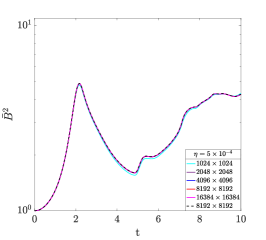
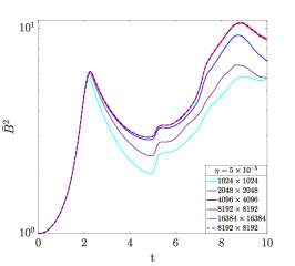
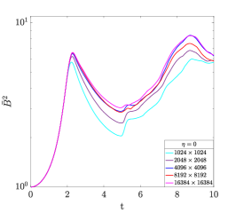
Figure 3: Evolution of the domain-averaged magnetic energy density $\bar{B}^{2}$ for $S=2\times 10^{3}$ (left), $S=2\times 10^{4}$ (middle), and the ideal case $\eta=0$ (right) for all resolutions considered.

2.2 Plasmoid formation

The initial magnetic field topology of the vortex is characterized by four alternating X-points and magnetic nulls, resulting in two magnetic islands along horizontal lines $y=0$ and $y=\pi$. The vortex motion immediately displaces the left island at $y=\pi$ diagonally upwards and the right island diagonally downwards, resulting in diagonal current sheets. The sheets get compressed, and depending on the Lundquist number, they can become tearing unstable, demonstrating the break-up in a series of plasmoids (see e.g., also van der Holst et al. 2008).

For $S\geq 10^{4}$ the current sheets shrink until they become plasmoid-unstable. In Figure 1 we show the rest-mass density $\rho$ for $S=10^{5}$ at $t=10t_{\rm c}$, where plasmoids are recognized as over-dense blobs of plasma in the thin current sheets. The current sheet is characterized by an anti-parallel magnetic field configuration resulting in a large out-of-plane component of the current density in the fluid frame,

$$\mathbf{J}=\eta^{-1}\Gamma[\mathbf{E}+\mathbf{v}\times\mathbf{B}/c-(\mathbf{E}\cdot\mathbf{v})\mathbf{v}/c^{2}],$$ (3)

as can be seen in the middle and right panels of Figure 2 for $S=2\times 10^{4}$ and resolution $8192^{2}$. For lower Lundquist numbers $S<10^{4}$ the current sheet does not become thin enough for the plasmoid instability to grow (see e.g., left panel of Figure 2 for $S=2\times 10^{3}$ and resolution $8192^{2}$).

2.3 Convergence of numerical results

We claim converged results if the evolution of the domain-averaged magnetic energy density $\bar{B}^{2}\equiv\frac{\iint_{V}B^{2}dxdy}{\iint_{V}dxdy}$ does not change anymore between successive doubling of the number of grid cells per direction over the full domain $V$ (see Figure 3). The plasmoid-unstable cases ($S\geq 10^{4}$) are most demanding and effective resolutions of $8192^{2}$ cells are needed to resolve the current sheets by at least 10 cells over their width. For our fiducial case of $S=2\times 10^{4}$ there are no visual differences between runs with resolutions of $8192^{2}$ and $16384^{2}$ grid cells (see middle panel of Figure 3). For lower resolutions $<8192^{2}$ the (average) magnetic energy density is underestimated (particularly after $t=2t_{\rm c}$) and the dissipation is governed by numerical resistivity that is larger than the explicit resistivity $\eta=5\times 10^{-5}$, affecting the energetics, heating, and plasmoid statistics. We also ensure that the effect of the AMR on the evolution of $B^{2}$ is negligible compared to a (significantly more expensive) run with uniform resolution of $8192^{2}$ grid cells (see the dashed black lines in the left and middle panels of Figure 3).

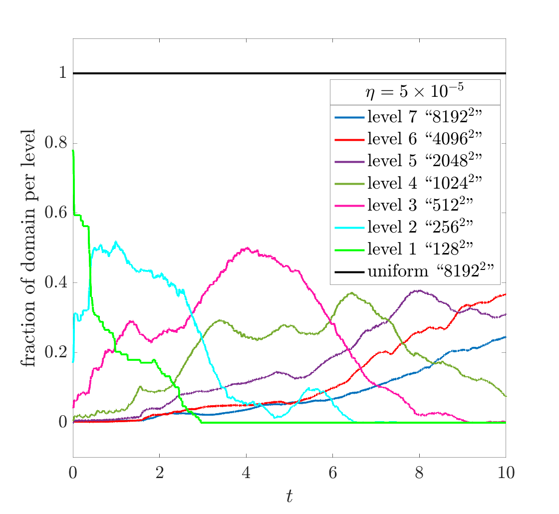
Figure 4: The time-evolution of the fraction of the domain covered by the individual AMR levels $n$, calculated as $\mathrm{cells}\times 4^{n_{\mathrm{max}}-n}$ with $n_{\mathrm{max}}=7$ levels, corresponding to an effective resolution of $8192^{2}$ for $S=2\times 10^{4}$. The black solid line indicates a run with a uniform grid of $8192^{2}$.

In Fig. 4 we show the fraction of the domain, calculated as the number of $\mathrm{cells}\times 4^{n_{\rm max}-n}$, with $n$ the AMR level and $n_{\rm max}$ the maximum number of levels, that is covered by the different AMR levels in time for $S=2\times 10^{4}$. It is clear that the lowest levels, 1 and 2, corresponding to an effective resolution of $128^{2}$ and $256^{2}$ respectively, are only important in the first part of the simulation $t<3t_{\rm c}$ (i.e., when the plasmoid instability is not yet activated). In the turbulent final stage of the simulation, less than 25% of the domain is covered by the highest level corresponding to an effective resolution of $8192^{2}$, and less than 40% by level 6, corresponding to an effective resolution of $4096^{2}$, resulting in a major speed-up compared to a uniform resolution of $8192^{2}$. The highest level is only activated around current sheets, as can also be seen in the right panel of Figure 2.

We performed an ideal GRMHD (i.e., $\eta=0$) run (see the right panel of Figure 3), showing that in this case the magnetic energy density evolution, and hence the (numerical) dissipation and heating of the plasma, does not converge even for the highest resolutions considered. Due to the absence of a resistive dissipation scale set by $\eta>0$ the current sheet shrinks to the grid scale, and is captured by one grid cell over its width for all resolutions considered here. Notice that the evolution of $B^{2}$ for $4096^{2}$ and $16384^{2}$ grid cells seems comparable for $\eta=0$, whereas the magnetic energy density is clearly lower for the case with $8192^{2}$ cells. The lowest resolution ($1024^{2}$) considered here is generally high enough to capture the essential (non-resistive) effects of the magnetorotational instability (MRI, Velikhov 1959; Chandrasekhar 1960; Balbus & Hawley 1991), the accretion dynamics, and the Blandford-Znajek jet launching process (Blandford & Znajek 1977) in global disk simulations according to recent studies in ideal GRMHD (Porth et al. 2019; White et al. 2019). One can see that at resolutions $<1024^{2}$, there is hardly a difference between the ideal and $S=2\times 10^{4}$ resistive results (cyan line in middle and right panels of Figure 3), and the linear growth phase of the magnetic energy density (at $t\lesssim 3t_{\rm c}$, i.e., where no plasmoids have formed yet) is accurately captured, confirming that numerical resistivity due to the finite grid dominates the magnetic energy dissipation and that higher resolutions are needed to resolve magnetic reconnection and plasmoid formation. For $S=2\times 10^{3}$ the evolution of the current sheet is easier to capture because the violent tearing instability is not triggered and the explicit resistivity is always larger than the numerical resistivity in this case. The resistive scale is already fully resolved for an effective resolution of $1024^{2}$ cells (see the left panel of Figure 3) and the sheet does not shrink below the threshold for plasmoid formation (see the left panel of Figure 2).

2.4 Reconnection rate

We analyze the reconnection rate for all considered Lundquist numbers in the converged runs by measuring the inflow velocity into the current sheet. In order to determine the inflow speed we use the upstream $\mathbf{E}\times\mathbf{B}$-velocity such that $v_{\rm up}/c=E_{z,\rm up}/B_{\rm up}$. We take five slices across the current sheet (ensuring that the slice does not cut across a plasmoid) at $t=10t_{\rm c}$ for all cases with resolutions of $16384^{2}$ such that even the thinnest sheet for $S=10^{5}$ is resolved. We then obtain a profile of $B_{\rm up}$ by projecting the magnetic field along the current sheet and find the location where the profile becomes flat (see the bottom panel of Figure 5 for $S=2\times 10^{4}$). We measure both the upstream electric and magnetic fields by averaging over 5 locations in the upstream on the slices on both sides of the sheet. We account for the bulk flow velocity ($v_{\rm bulk}\ll c$ such that $\Gamma_{\rm bulk}=1$) of the vortex by defining the speed on the left of the sheet as $v_{\rm up,left}/c=(v_{\rm bulk}+v_{\rm in}$)/c and on the right of the sheet as $v_{\rm up,right}/c=(v_{\rm bulk}-v_{\rm in})/c$, such that $v_{\rm rec}/c=(v_{\rm up,left}-v_{\rm up,right})/2c$. Assuming that the outflow $v_{\rm out}=v_{A}\approx c$, this directly yields the reconnection rate $v_{\rm rec}/c=v_{\rm in}/v_{\rm out}=v_{\rm in}/c$. We confirmed that locally, in the upstream region of the current sheet, $\sigma=b^{2}/(\rho hc^{2})\approx 8$ such that the Alfvén speed around the sheet is $v_{A}=c(\sigma/(\sigma+1))^{1/2}\approx c$ and that the reconnection is relativistic. In the top panel of Figure 5 we observe a Sweet-Parker scaling $v_{\rm rec}/c\sim S^{-1/2}$ for $S<10^{-4}$ (indicated by the blue circles and the dashed black line) and plasmoid-dominated “fast” reconnection with a rate independent of the Lundquist number of $v_{\rm rec}/c\approx 0.01$ for $S\geq 10^{4}$ (indicated by the red circles and the dotted black line).

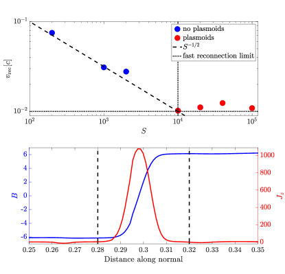
Figure 5: Top panel: Reconnection rate (blue circles) measured as $v_{\rm rec}/c=(v_{\rm up,left}-v_{\rm up,right})/2c$ versus the Lundquist number $S$, showing a Sweet-Parker scaling $v_{\rm rec}/c\sim S^{-1/2}$ (dashed black line) for $S<10^{4}$. For $S\geq 10^{4}$ we observe a “fast” reconnection rate (red circles) that is independent of the Lundquist number, as indicated by the dotted back line. Bottom panel: In-plane magnetic field $B$ projected along the sheet (blue line) and out-of-plane current density $J_{z}$ (red line) profiles taken on a slice through the current sheet in the right panel of Figure 2 for $S=2\times 10^{4}$. The magnetic field geometry shows a typical Harris-like current sheet profile. We define the upstream, where we sample the reconnection rate averaged over 10 neighbouring grid cells, to the left and right of the dashed black lines.

3 Magnetic reconnection and plasmoid formation in black-hole accretion flows

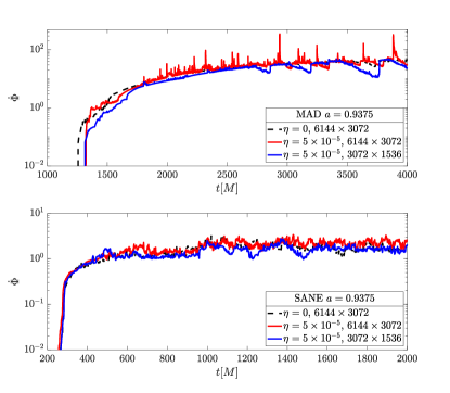
Figure 6: Time-evolution of the magnetic flux through the horizon $\dot{\Phi}$ for a MAD run (top) and a SANE run (bottom) for $\eta=0$ (dashed black lines) and $\eta=5\times 10^{-5}$ (solid red lines). The ideal and resistive results at a resolution of $6144\times 3072$ are in agreement and the global accretion dynamics are unaffected by resistivity. We also show the resistive run at a resolution that is twice smaller per direction, $3072\times 1536$ (blue lines), to show convergence of the global accretion dynamics.

It is much harder to localize and track the formation of current sheets in realistic black-hole accretion flows in a larger domain and for a longer period because of the effects of the more complicated global dynamics governed by the central object, and due to the turbulence induced by the MRI. Both the evolution of accretion flows and the formation of current sheets therein strongly depend on the magnetic field geometry. We model an accretion disk around a rotating black hole varying the initial conditions to study current sheet formation in different scenarios of magnetic field geometry. In the Magnetically Arrested Disk (MAD, Igumenshchev et al. 2003; Narayan et al. 2003) scenario the MRI and subsequent turbulence in the inner accretion disk are suppressed due to large-scale magnetic flux (see e.g., White et al. 2019). In axisymmetric simulations as considered here, the arrested inflow is regularly broken by frequent bursts of accretion, allowing for a macroscopic equatorial current sheet to form and break in a periodic fashion. In a full 3D setup magnetically buoyant structures are interchanged with less-magnetized dense fluid (Igumenshchev 2008; White et al. 2019), resulting in a magnetic Rayleigh-Taylor instability (Kruskal & Schwarzschild 1954) potentially sourcing interchange-type magnetic reconnection. In the Standard And Normal Evolution (SANE, Narayan et al. 2012; Sadowski et al. 2013) state a fully turbulent accretion disk can develop due to a smaller magnetic flux (see e.g., Porth et al. 2019), and current sheets can ubiquitously form and interact with the turbulent flow. Polarized synchrotron radiation observed by the Event Horizon Telescope (EHT, Event Horizon Telescope Collaboration et al. 2019a) can probe the field line structure at event-horizon scales and put tighter constraints on the magnetization and address whether the accretion is in a SANE or a MAD state (Event Horizon Telescope Collaboration et al. 2019b).

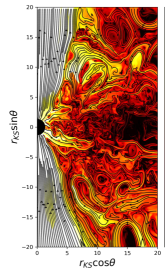
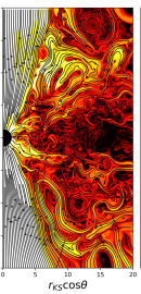
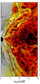
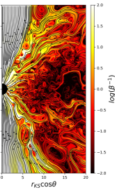
Figure 7: $\beta^{-1}=b^{2}/(2p)$ at four typical times $t=[1460,1480,1540,1580]r_{g}/c$ (from left to right) during quasi-state-state phase of accretion in the SANE configuration. Magnetic field lines plotted are on top as solid black lines. In the bottom half one can detect the accretion of a magnetic flux tube at $r_{KS}\cos\theta=x\approx 6r_{g},r_{KS}\sin\theta=y\approx-8r_{g}$ (left two panels) that inflates, opens up and becomes tearing unstable (third panel) after it connects to the black hole, and produces copious plasmoids coalescing into large-scale structures at $x\approx 5r_{g},y\approx-10r_{g}$ (fourth panel) with a typical size of about one Schwarzschild radius. In the top half of the panels a similar process can be seen at $x\approx 7r_{g},y\approx 13r_{g}$ in the second and third panel, also resulting in a large-scale plasmoid at $x\approx 9r_{g},y\approx 18r_{g}$ in the fourth panel.

Here, we consider both the SANE and MAD scenarios, studying whether forming current sheets can become tearing-unstable and produce macroscopic plasmoids before breaking up. We also investigate how large these plasmoids can grow and whether they are bounded to the disk or expelled from the disk, e.g., along the jet’s sheath.

3.1 Numerical setup

We consider both MAD and SANE magnetic field configurations around a Kerr black hole, for three representative values of the dimensionless spin parameter $a\in[-0.9375;0;0.9375]$, corresponding to near-extremal retrograde Kerr, Schwarzschild, and near-extremal prograde Kerr black holes, respectively. We use geometrized units with gravitational constant, black-hole mass, and speed of light $G=M=c=1$; such that length scales are normalized to the gravitational radius $r_{g}=GM/c^{2}$ and times are given in units of $r_{g}/c$. We employ spherical Kerr-Schild coordinates, where $r$ is the radial coordinate, $\theta$ and $\phi$ are the poloidal and toroidal angular coordinates, respectively, and $t$ is the temporal coordinate. We start our simulations from a torus in hydrodynamic equilibrium (Fishbone & Moncrief 1976) threaded by a single weak poloidal magnetic field loop, defined by the vector potential

$$A_{\phi}\propto\max(q,0),$$ (4)

where the function $q$ is set to obtain a large torus resulting in a MAD state:

$$q=\frac{\rho}{\rho_{\rm max}}\left(\frac{r}{r_{\rm in}}\right)^{3}\sin^{3}\theta\exp\left(-\frac{r}{400}\right)-0.2,$$ (5)

with an inner radius $r_{\rm in}=20r_{g}$ and the density maximum $\rho_{\rm max}$ is located at $r_{\rm max}=41r_{g}$ for $a=0.9375$, $r_{\rm max}=42r_{g}$ for $a=-0.9375$, and $r_{\rm max}=41.4r_{g}$ for $a=0$ to start from an initial torus of similar size. For a SANE state we set a smaller torus with

$$q=\frac{\rho}{\rho_{\rm max}}-0.2,$$ (6)

where the inner radius $r_{\rm in}=6r_{g}$ and the density maximum $\rho_{\rm max}$ is located at $r_{\rm max}=12r_{g}$ for $a=0.9375$, $r_{\rm max}=22r_{g}$ for $a=-0.9375$, and $r_{\rm max}=15r_{g}$ for $a=0$ to start from an initial torus of similar size. In both cases the magnetic field strength is set such that $\beta=2p_{\rm max}/b^{2}_{\rm max}=100$. Plasma-$\beta$ and the magnetization $\sigma=b^{2}/(\rho c^{2})$ for a cold (i.e., $p\ll\rho$) plasma are defined using the magnetic field strength $b^{2}$ co-moving with the fluid (see Ripperda et al. 2019c for a definition). We set an atmospheric rest-mass density and pressure as $\rho_{\rm atm}=\rho_{\rm min}r^{-3/2}$ and $p_{\rm atm}=p_{\rm min}r^{-5/2}$ where $\rho_{\rm min}=10^{-4}$ and $p_{\rm min}=10^{-6}/3$. We apply floors on rest-mass density, pressure, and Lorentz factor $\Gamma<\Gamma_{\rm max}=20$ such that the magnetization $\sigma=b^{2}/(\rho c^{2})<\sigma_{\rm max}=100$ and $\beta^{-1}=b^{2}/2p<\beta^{-1}_{\rm max}=(10\sigma_{\rm max})^{(\hat{\gamma}-1)}$. We adopt an equation of state for a relativistic ideal gas with an adiabatic index of $\hat{\gamma}=4/3$. The equilibrium fluid pressure is perturbed to trigger the MRI as $p=p_{\rm eq}(1+X_{p})$ with a random variable uniformly distributed between $X_{p}\in[-0.02;0.02]$.

We model dissipation in the accretion flow by assuming a small, uniform, and constant resistivity $\eta=5\times 10^{-5}$ in the set of GRRMHD equations (Ripperda et al. 2019c), resulting in a large Lundquist number $S=Lc/\eta\sim 2\times 10^{5}$ that is well above the plasmoid threshold, where we assume the typical length scale to be the length of a current sheet $L=L_{\rm{sheet}}\sim\mathcal{O}(10r_{g})$, and the speed of light $c$ as the typical velocity. A small resistivity allows us to capture both the global near-ideal accretion dynamics (Ripperda et al. 2019c) and the fast reconnection resulting in plasmoid formation in localized thin current sheets (Ripperda et al. 2019b).

3.2 Convergence of numerical results

We show in Figure 6 that both MAD and SANE configurations in ideal and resistive runs reach a quasi-steady-state after approximately $2500r_{g}/c$ and $500r_{g}/c$ respectively, as indicated by the magnetic flux through the horizon:

$$\dot{\Phi}:=\frac{1}{2}\int_{0}^{2\pi}\int^{\pi}_{0}|B^{r}|\sqrt{-\gamma}d\theta d\phi,$$ (7)

where $\gamma$ is the determinant of the spatial part of the metric.

Figure 6 shows the magnetic flux for the highest resolution considered, $6144\times 3072$ cells, compared to a resolution of $3072\times 1536$, confirming that quasi-steady-state phase of accretion is independent of the resolution in our simulations. We confirm convergence of the thinning process of the current sheets by restarting from the quasi-steady-state increasing the resolution up to $12288\times 6144$, and measure the cells per thickness of the sheets. In all considered cases the sheets are captured by 8 or more cells over their widths, which is discussed in section 3.3.

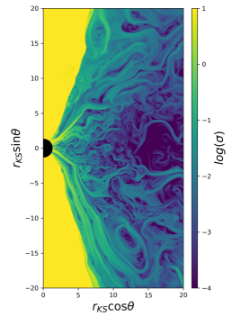
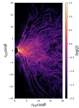
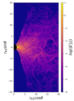
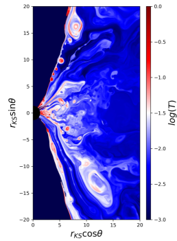
Figure 8: Representative SANE snapshot in quasi-steady-state phase of accretion at $t=1540r_{g}/c$. top-left: Magnetization $\sigma$ showing that current sheets along the jet’s sheath are in the relativistic regime $\sigma\gg 1$, whereas in the disk they are in the transrelativistic regime $\sigma\lesssim 1$. top-right: The thin tearing-unstable reconnection layers are indicated by a strong current density. bottom-left: Plasmoids in the current sheets are heated by Ohmic heating close to the event horizon. bottom-right: Plasmoids both in the disk and along the jet’s sheath are heated up to relativistic temperatures $T=p/\rho\sim 1$.

3.3 Plasmoid formation in the SANE model

Current sheets are expected to form above the disk or in the jet’s sheath where magnetic flux tubes are twisted by global shearing motion. These structures can inflate while they accrete onto the black hole and get thinner after which their magnetic energy is dissipated close to the event horizon through reconnection. The magnetic energy is released into heat and bulk motion of the plasmoids that can either fall into the black hole or get ejected. This process has been studied in the force-free paradigm, assuming the plasma to be infinitely magnetized (Parfrey et al. 2014; Yuan et al. 2019a, b; Mahlmann et al. 2020). Additionally, when the net magnetic flux in the accretion disk is relatively small, turbulence resulting from the MRI can produce magnetic fields with alternating polarities prone to reconnection (Davis et al. 2010; Zhu & Stone 2018). MHD turbulence is known to intermittently form large plasmoid-unstable current sheets (Zhdankin et al. 2013, 2017; Dong et al. 2018) and the plasmoid instability can significantly modify the turbulent MHD cascade at relatively small scales and high Lundquist numbers $S\sim 10^{6}$ (Boldyrev & Loureiro 2017; Comisso et al. 2018; Dong et al. 2018).

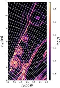
Figure 9: Zoom into a current sheet (see top-right panel of Figure 8), showing plasmoids that are advected along the jet’s sheath and reached a typical size of the order of a few Schwarzschild radii through coalescence. The over-plotted grid-block structure (white rectangles) shows that each current sheet is captured by approximately 10 cells over its width. Each block represents $64\times 32$ cells.

In Figure 7 we observe both processes in a SANE configuration and detect current sheets in the disk and along the jet’s sheath, indicated by a small $\beta^{-1}$ and anti-parallel field lines. In the left-most two panels at $t=1460r_{g}/c$ and $t=1480r_{g}/c$ a large flux tube falls onto the black hole in the left bottom half at approximately $x=r_{\rm KS}\cos\theta\approx 8r_{g}$, $y=r_{\rm KS}\sin\theta\approx-8r_{g}$. In the third panel, at $t=1540r_{g}/c$, the flux tube has both its footpoints attached to the black hole, it opened up after it inflated and became thin enough to be tearing unstable and form multiple plasmoids (Parfrey et al. 2014 observe a similar process). In the fourth panel, at $t=1580r_{g}/c$, the plasmoids that are advected away from the black hole along the jet’s sheath have formed a large structure at $x\approx 6r_{g},y\approx-10r_{g}$ through coalescence. At $x\approx 9r_{g},y\approx 17r_{g}$ a similar process occurs in the third panel and a large plasmoid has formed through mergers of multiple smaller plasmoids that can be seen in the left panels. In the first and second panel one can detect a flux tube with one footpoint connected to the black hole, that is then twisted by the shear flow, becomes thinner and inflates, at $x\approx 3r_{g},y\approx 2r_{g}$, after which it ejects plasmoids into the accretion disk in the fourth panel at $x\approx 6r_{g},y\approx 2r_{g}$. A similar process occurs in the first panel for a loop with one footpoint on the black hole at $x\approx 7r_{g},y\approx-2r_{g}$. The large-scale plasmoids form on a time scale of $\sim\mathcal{O}(100r_{g}/c)$ growing to circular objects with a radius $\gtrsim\mathcal{O}(r_{g})$, indicating a reconnection rate of $\approx 0.01c$. These structures eventually break up and lose coherence due to interaction with the ambient flow.

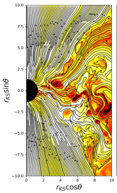
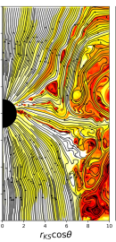
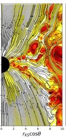
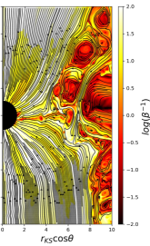
Figure 10: $\beta^{-1}=b^{2}/(2p)$ at four typical times $t=[2941,2971,2988,3009]r_{g}/c$ (from left to right) during the quasi-state-state phase of accretion in the MAD configuration. Magnetic field lines are plotted on top as solid black lines. In the top half one can detect the accretion of a magnetic flux tube (left panel) at $x\approx 3r_{g},y\approx 1r_{g}$ that opens up and becomes tearing unstable (second panel) after it connects to the black hole, and produces copious plasmoids coalescing into large-scale structures (third and fourth panels at $x\approx 5r_{g},y\approx 2.5r_{g}$ with a typical size of about one Schwarzschild radius.

In Figure 8 we show the magnetization $\sigma=b^{2}/(\rho c^{2})$, temperature $T=p/\rho$, magnetic dissipation $|E^{i}J_{i}|$, and the current density magnitude $J=\sqrt{J^{i}J_{i}}$, where $E^{i}$ and $J^{i}$ are the Eulerian electric field and current density (see Ripperda et al. 2019c for definitions) at $t=1540r_{g}/c$ (the third panel in Figure 7). We mask the regions with $\sigma\geq 5$ where the flow dynamics is dominated by the density and pressure floors. In the top-right panel one can detect ubiquitous current sheets along the jet’s sheath and inside the disk within $10r_{g}$, indicated by a strong current density. The current sheets are tearing-unstable and plasmoids form close to the event horizon after which they either fall into the black hole, or are advected along the jet’s sheath, merge with other plasmoids, and grow into larger objects with a size of the order of a few $r_{g}$. The magnetization in the top-left panel shows that current sheets along the jet’s sheath reconnect in a highly relativistic regime (i.e., $\sigma\gg 1$), whereas in the disk reconnection occurs in the transrelativistic regime $\sigma\lesssim 1$. Reconnection in the highly magnetized plasma surrounding the jet’s sheath and the current sheets in the equatorial plane efficiently heats plasmoids to relativistic temperatures $T=p/\rho\sim 1$ as can be seen in the bottom-right panel. These hot plasmoids are advected along the jet’s sheath or into the accretion disk. Heating of plasmoids that form inside the disk due to reconnection induced by MRI turbulence is less efficient due to the low magnetization in the disk. Instead, hot plasmoids observed at $x\approx 6r_{g},y\approx\pm 2r_{g}$ were energized in the inner region close to the event horizon and ejected into the disk. The plasmoids are mainly heated close to the event horizon by Ohmic heating as can be seen from the bottom-left panel. The strong parallel electric field indicated by $|E^{i}J_{i}|$ in the bottom-left panel can potentially accelerate particles to non-thermal energies.

Figure 9 shows a zoom into the current sheet along the jet’s sheath with several interacting plasmoids as visible Figure 8. The current sheets are captured by typically 10 cells along their widths, as can be seen from the on-plotted grid-block structure (white rectangles), where each block consists of $64\times 32$ cells.

3.4 Plasmoid formation in the MAD model

In a MAD configuration the accretion disk is threaded by a strong magnetic flux suppressing the MRI and forming a more powerful magnetized jet than in the SANE case. In Figure 10 we show the typical evolution of a current sheet indicated by a small $\beta^{-1}$ in the highly magnetized equatorial region close to the black hole at representative times $t=[2941,2971,2988,3009]r_{g}/c$ (from left to right). In the left panel a magnetic flux tube falls onto the black hole at $x\approx 1r_{g},y\approx 3r_{g}$ and in the second panel the tube connects its two footpoints to the black hole. A near-equatorial current sheet forms and produces multiple small plasmoids within $5r_{g}$ from the event horizon. The plasmoids that escape the gravitational pull merge into a large structure in the third panel at $x\approx 6r_{g},y\approx 2.5r_{g}$. The large-scale plasmoid grows to a circular structure with a radius $\gtrsim 1r_{g}$ and escapes along the jet’s sheath at $x\approx 9r_{g},y\approx 6r_{g}$ in the fourth panel. The process of formation to ejection takes place on a time scale of $\sim 70r_{g}/c$. In the fourth panel the process restarts with an in-falling flux tube at $x\approx 9r_{g},y\approx 0r_{g}$.

In Figure 11 we show the magnetization, current density, Ohmic heating, and temperature for the MAD state, where we again mask the regions with $\sigma\geq 5$. Due to the higher magnetization (see the top-left panel) surrounding the equatorial current sheets (see the top-right panel) in the MAD state, the plasmoids are heated to relativistic temperatures $T\sim 10$ (bottom-right panel), an order of magnitude higher than in the SANE case. The current density in the sheets is significantly higher than in the SANE case. The plasmoids are heated through Ohmic heating close to the event horizon, as can be seen from the bottom-left panel.

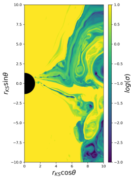
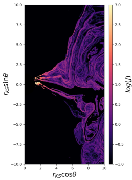
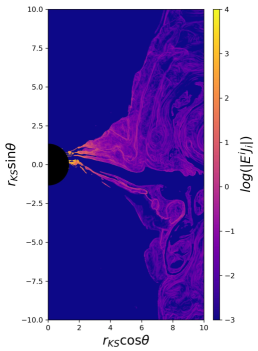
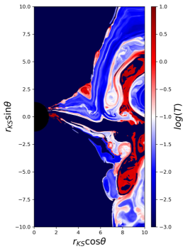
Figure 11: Representative MAD snapshot in the quasi-steady-state phase of accretion at $t=2971r_{g}/c$. top-left: Magnetization $\sigma$ showing that current sheets close to the event horizon are in the relativistic regime $\sigma\gg 1$. top-right: The thin tearing-unstable reconnection layers are indicated by a strong current density. bottom-left: Plasmoids in the current sheets are heated by Ohmic heating close to the event horizon. bottom-right: Plasmoids formed in the equatorial sheets are advected into both the disk and along the jet’s sheath and are heated up to relativistic temperatures $T=p/\rho\sim 10$, an order of magnitude larger than in the SANE case in Figure 8.

3.5 Reconnection rate

We calculate the reconnection rate in a similar way as for the Orszag-Tang vortex for both MAD and SANE configurations. We first transform the Eulerian electric and magnetic fields into a local inertial frame (see e.g., White et al. 2016) to apply the standard reconnection analysis. We project the fields in the flat frame along the direction parallel to the current layer to determine the upstream geometry, and a typical Harris-type sheet structure is found in Figure 12 both for the magnetic field and the current density magnitude $J$. All three magnetic field components switch sign in the current sheets, indicating that zero-guide-field reconnection occurs in both MAD and SANE cases.

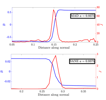
Figure 12: Magnetic field $B$ in a local inertial frame, projected along the sheet (blue line) and current density magnitude $J$ (red line) profiles taken on a slice through a current sheet in a MAD snapshot (top panel) and a SANE snapshot (bottom panel). The magnetic field geometry shows a typical current sheet profile.

In the local inertial frame we determine the inflow speed from the $\mathbf{E}\times\mathbf{B}$-velocity that we project along the direction perpendicular to the current sheet, and then calculate the reconnection rate as $v_{\rm rec}/c=(v_{\rm up,left}-v_{\rm up,right})/2c$. In both MAD and SANE configurations we select ten current sheets at different times during the quasi-steady-state phase of accretion and consistently find a reconnection rate between 0.01c and 0.03c. This finding is in accordance with analytic resistive MHD predictions for plasmoid-dominated reconnection in isolated current sheets (Bhattacharjee et al. 2009; Uzdensky et al. 2010). Note that the actual Lundquist number is approximately $S=L_{\rm{sheet}}c/\eta\gtrsim\mathcal{O}(10^{5})$, since all current sheets have a typical length scale of $\sim\mathcal{O}(5-20r_{g})$, confirming that reconnection occurs in the plasmoid-dominated regime as $S\gg 10^{4}$.

4 Flare analysis

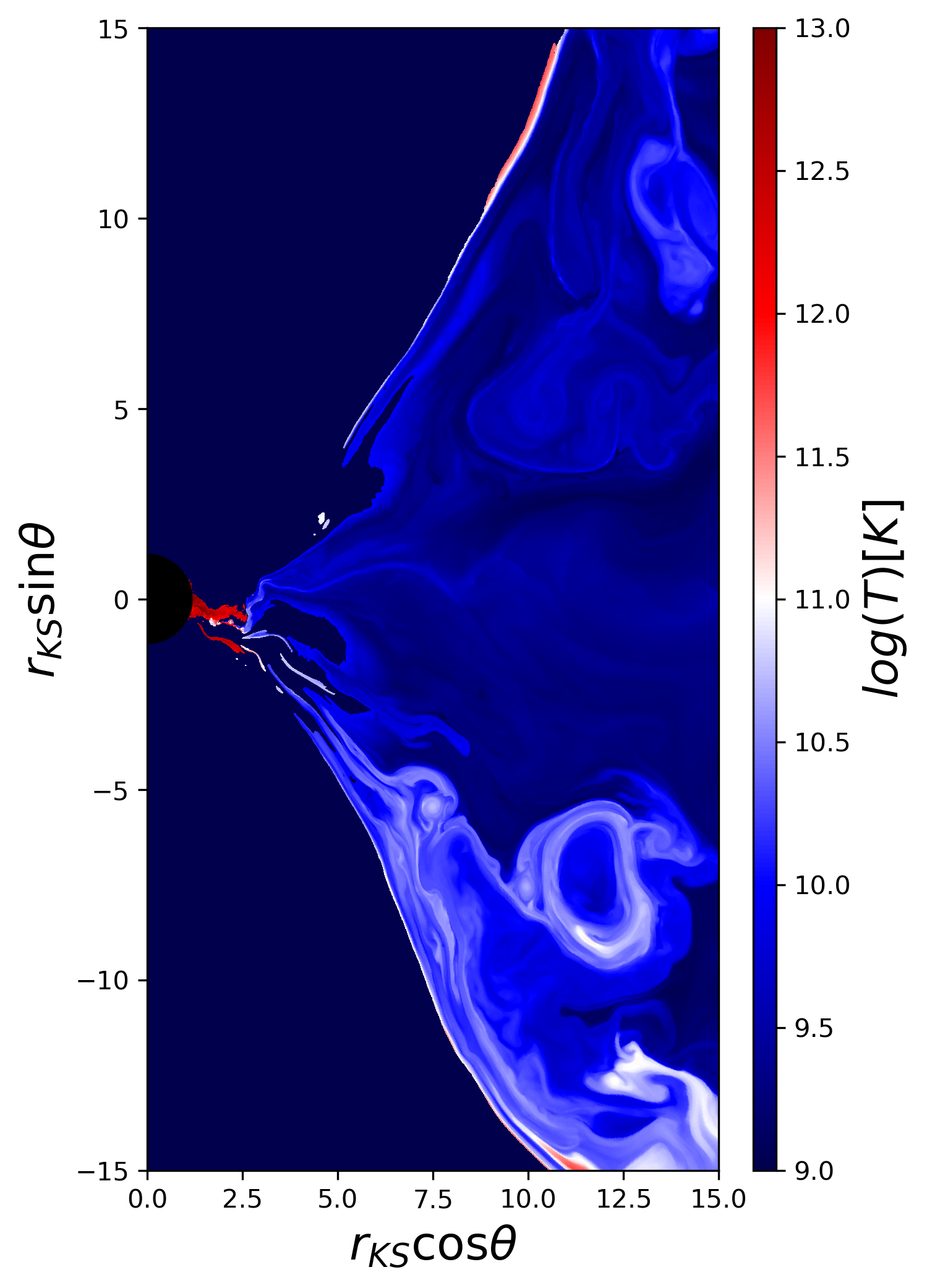
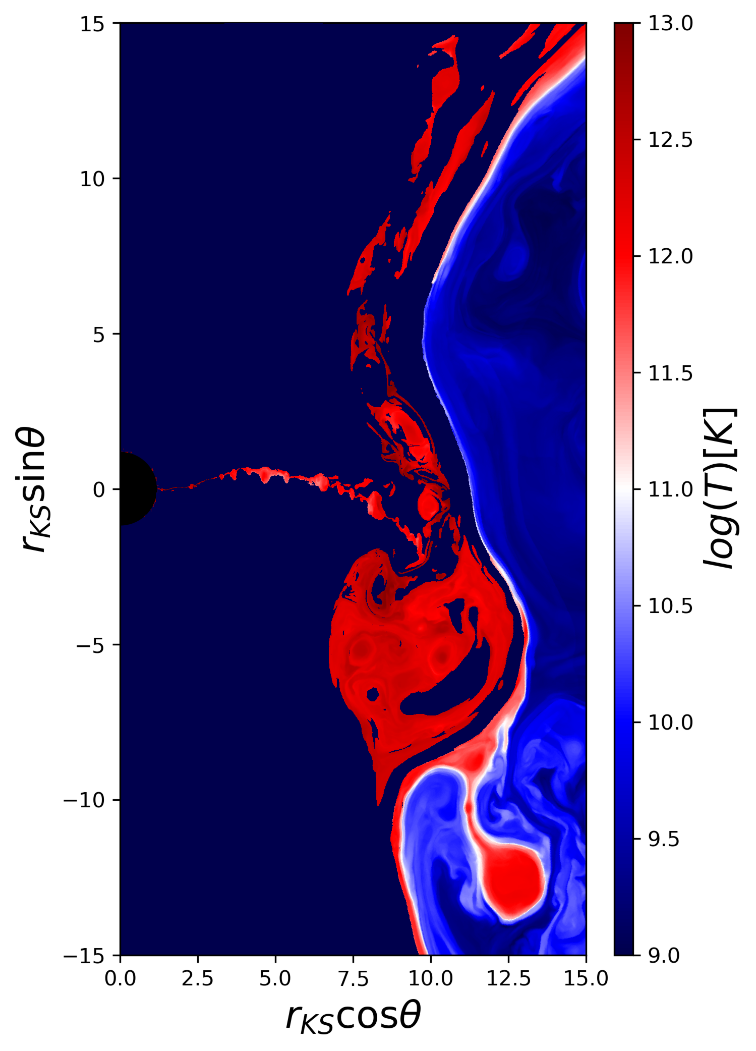
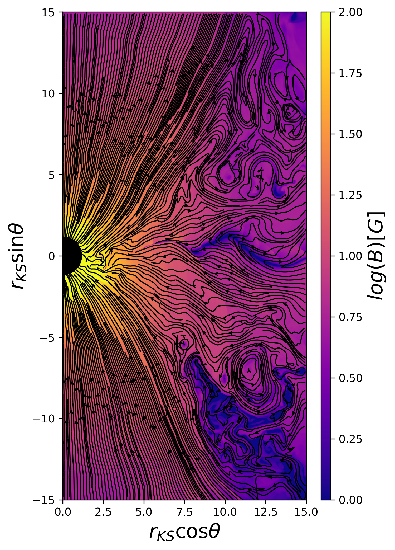
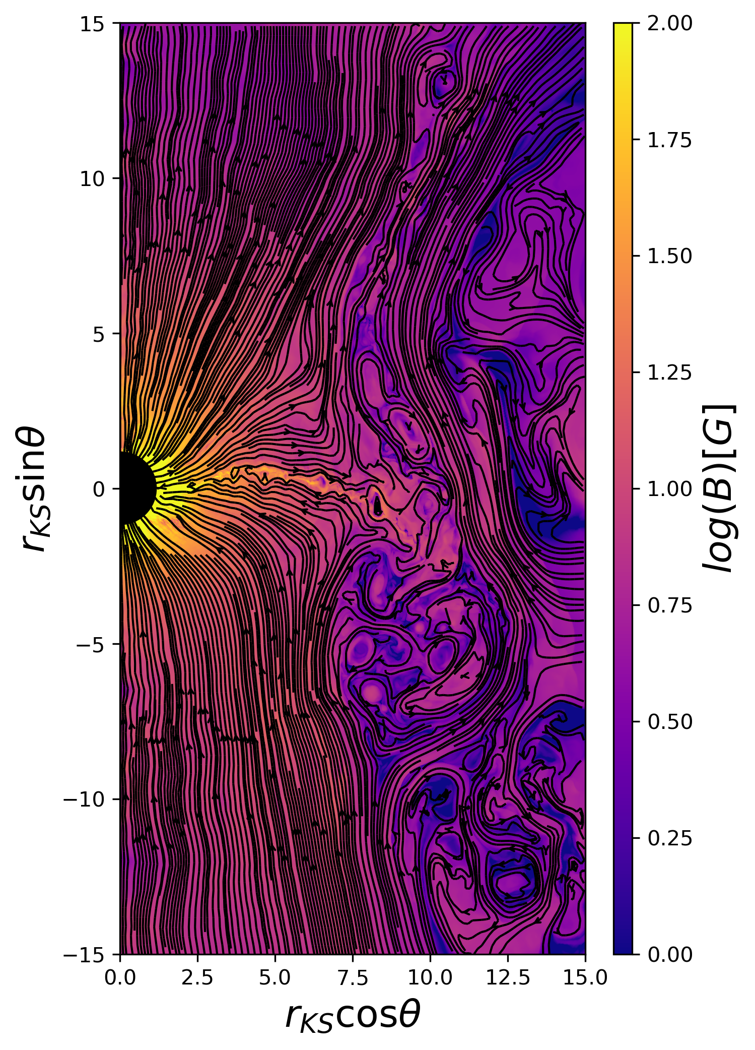
Figure 13: Representative prograde MAD snapshot for typical Sgr A^∗ parameters during quiescence (left panels) at $t=3155r_{g}/c$ and during a flaring state (right panels) at $t=3259r_{g}/c$. top-left: The temperature $T$[K] in quiescent state remains approximately $10^{10}$K in the disk. A remnant of a previous flare (see Fig. 11) can be detected at $x\approx 12r_{g},y\approx-9r_{g}$. top-right: A current sheet has formed at $y\approx 0r_{g}$, producing plasmoids that heat the jet’s sheath to temperatures $\gg 10^{10}$K through the reconnection exhaust. A hot spot with a radius of a few $r_{g}$ can be detected at $x\approx 8r_{g},y\approx-5r_{g}$. bottom-left: The magnetic field during quiescence decreases as $\propto r^{-1}$ from approximately 50G at the inner radius of the disk at $\sim 3r_{g}$ to 10G at $10r_{g}$. bottom-right: The equatorial current sheet shows a clear field reversal. In the hot spot that is fed by the plasmoids from the current sheet, the magnetic field strength has decreased to 1-5[G], indicative of a large flare.

Sgr A^∗ shows daily flares in the near-infrared (on average every $\sim 6$ hours, Eckart et al. 2006) and X-ray (on average every $\sim 12-24$ hours, Baganoff et al. 2003) spectrum, often without a significant time-lag. The X-ray flares are large-amplitude outbursts followed by a quiescent period, whereas near-infrared flares appear as peaks within an underlying noise. The near-infrared flares can typically last for $\sim 80$ minutes, and the X-ray flares show shorter time-scales of $\sim 50$ minutes. Sub-structural variability with a characteristic timescale of $\sim 15–25$ minutes is regularly observed in near-infrared flares (Genzel et al. 2003; Eckart et al. 2006. The Gravity Collaboration et al. (2018) resolved the flare locations of three flares in the central $10r_{g}$. The near-infrared flares are polarized, indicating their origin in synchrotron radiation produced by relativistic electrons. The polarization angle can change significantly during the flare (Dodds-Eden et al. 2009, 2010), indicating a change of topology of the magnetic field e.g., due to magnetic reconnection. The near-infrared flares in the spectrum are explained by a peak synchrotron frequency in accordance with Lorentz factors of $\Gamma\gtrsim 10^{3}(B/B_{\rm quiescence})^{-1/2}$, where $B$ is the magnetic field strength in Gauss [G] and $B_{\rm quiescence}\sim 10-50$G is the field strength in quiescent periods in the inner $10r_{g}$ of the accretion disk (Dodds-Eden et al. 2009). This in turn requires particle acceleration, which is likely to be powered by tapping energy from the magnetic field, to energies well above the quiescent temperature of $\sim 3\times 10^{10}$K (Bower et al. 2006). The magnetic field strength is expected to significantly decrease to $\sim 1-10$G during a flare, to explain the simultaneity and symmetry of the X-ray and near-infrared light-curves (Dodds-Eden et al. 2010).

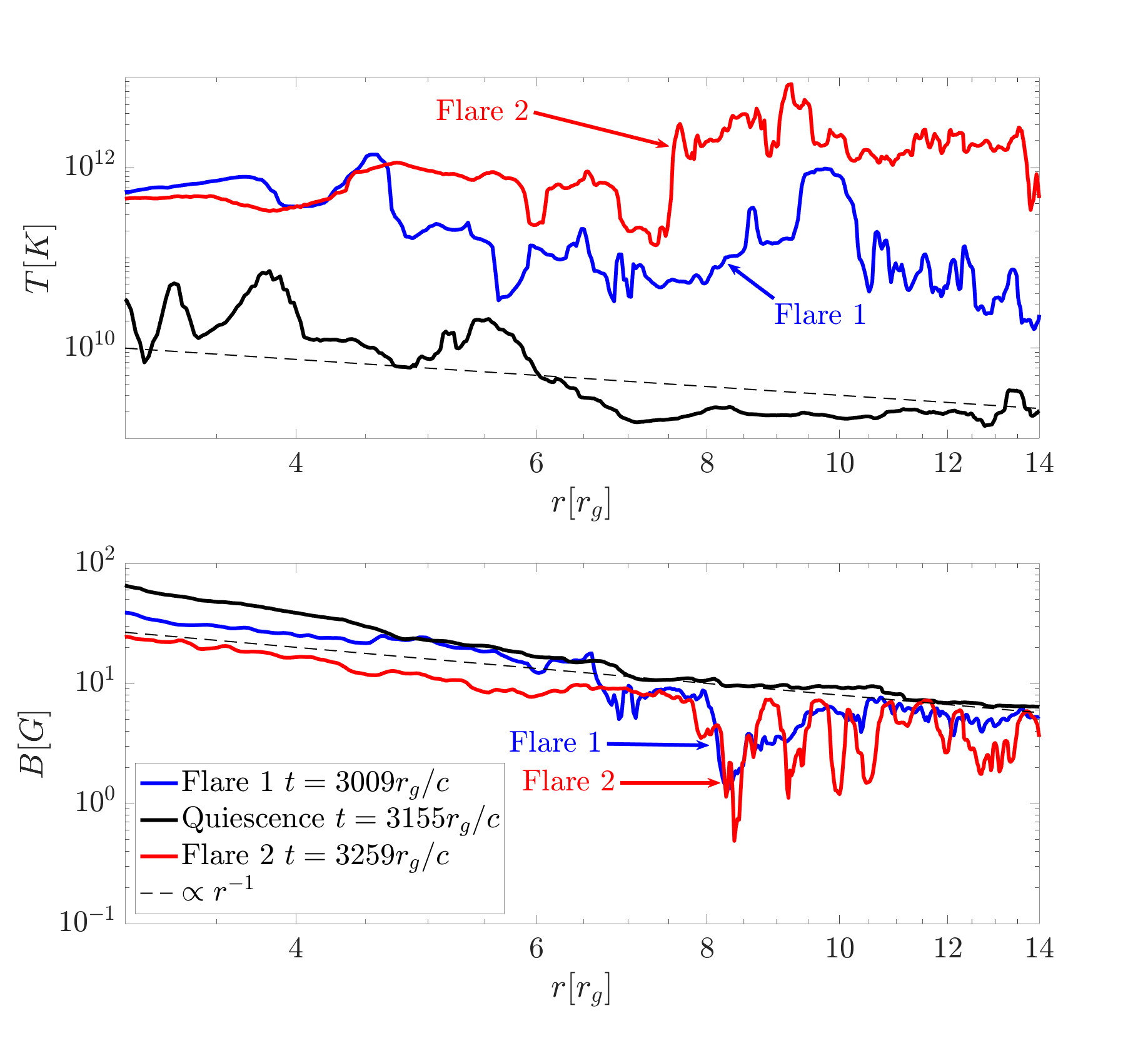
Figure 14: Radial cuts of the temperature $T$ and magnetic field strength $B$, assuming Sgr A^∗ parameters, of the flares in Figs. 10 (flare 1, at $t=3009r_{g}/c$) and 13 (flare 2, at $t=3259r_{c}/c$). The black lines show $T$ and $B$ during quiescence. The magnetic field shows a clear drop from $\sim 10-20$G to $\sim 1-5$G between $7r_{g}$ and $13r_{g}$, while the temperature significantly increases, both for flare 1 and 2.

Here, we compare the first time-dependent GRRMHD model for flare generation with observational constraints for Sgr A^∗. To convert the plasma temperature, and magnetic field strength from code units to c.g.s. units we find a scaling factor $B_{0}=50$G for the MAD state such that the field strength at $3r_{g}$, where the accretion disk starts, is equal to 50G in quiescence, as constrained by observations (Dodds-Eden et al. 2009) for Sgr A^∗. This results in a field strength of 10G at $10r_{g}$ in quiescence, and the field strength scales as $\propto r^{-1}$ with distance from the black hole. The fluid temperature $p/\rho$ is normalised as $T_{0}=p_{0}m_{p}/(\rho_{0}k_{B})$ [K], where $\rho_{0}=B_{0}^{2}/(4\pi c^{2}\sigma_{0})\rm{[g/cm^{3}]}$, $p_{0}=B_{0}^{2}\beta_{0}c^{2}/(2c^{2}4\pi){\rm[g/(cm\cdot s^{2})]}$, $\sigma_{0}=0.33$, $\beta_{0}=0.35$ (taken at $3r_{g}$), $m_{p}$ the proton mass, and $k_{B}$ Boltzmann’s constant in c.g.s. units., resulting in a quiescent temperature of $\sim 10^{10}$K at $10r_{g}$. Since the plasma is nearly collisionless, the electron temperature can be different from the temperature in the GRRMHD simulations, which has to be thought of as the proton temperature. For a normalization $\dot{M}_{0}=\rho_{0}r_{g}^{2}c^{3}/(MG)$ $\rm{[g/s]}$ we find a variable mass accretion rate of $\dot{M}\in[10^{-10},10^{-7}]M_{\odot}\rm{yr^{-1}}$ during the quasi-steady-state phase of accretion for both prograde and retrograde MAD simulations, consistent with bounds based on the measured Faraday rotation ruling out accretion rates greater than $\sim 10^{-7}M_{\odot}\rm{yr}^{-1}$ (Bower et al. 2003; Marrone et al. 2007). Note that we only determined a scaling factor $B_{0}$ for the magnetic field to find $\rho_{0}$, $p_{0}$, $T_{0}$ and $\dot{M}_{0}$, without relying on any other assumptions.

In Figure 13 we show the magnetic field $B$ [G] (bottom panels) and the temperature $T$ [K] (top panels) in quiescence (left panels) and during a flaring state (right panels). The temperature clearly increases by several orders of magnitude during a flare (top-right panel), and a hot spot forms at $x\approx 8r_{g},y\approx-5r_{g}$. The hot spot is fed by plasmoids from the exhaust of the equatorial current sheet at $x\approx 8r_{g},y\approx 0r_{g}$. The plasmoids heat the jet’s sheath, potentially explaining the mechanism behind limb-brightening which is for example observed down to $7r_{g}$ in the jet of the supermassive black hole in the center of the M87 galaxy (Ly et al. 2007; Kim et al. 2018). The magnetic field clearly shows field reversal at the current sheet at $y\approx 0r_{g}$, and a decrease to $\sim 1-5$G in the hot spot. In quiescence the temperature remains of the order of $10^{10}$K in the inner $10r_{g}$ (top-left panel), except in the inner $1r_{g}$, where a new current sheet forms. A remnant of a previous flare (shown in 11) can be detected at $x\approx 12r_{g},y\approx-9r_{g}$, and at $x\approx 14r_{g},y\approx 10r_{g}$ in the left panels.

In Fig. 14 we show the temperature (top panel) and the magnetic field strength (bottom panel) along a radial cut for two consecutive flares; The first one (the blue line) corresponds to the hot spot at $x\approx 7r_{g},y\approx 6r_{g}$ in Fig. 10 at $t=3009r_{g}/c$; Then a quiescent period follows (corresponding to the black line, at $3155r_{g}/c$); And then a second flare (the red line) at $x\approx 8r_{g},y\approx-5r_{g}$, corresponding to the hot spot in Fig. 13. Both flares originate from hot spots that have a radius of $\sim 1-3r_{g}$, last for approximately $\sim 30-45$ minutes, and show clear substructure as a result from individual large plasmoids in the turbulent exhaust of the current sheet. The magnetic field drops within $\sim 10-15$ minutes from $10-50$G in quiescence to $\sim 1-5$G during a flare. This is consistent with a scenario where the synchrotron emission is produced by a non-thermal distribution of electrons, accelerated by energy that is tapped from the magnetic field via reconnection, following the analyses of Dodds-Eden et al. (2010) and Ponti et al. (2017) of multi-wavelength observations of the X-ray and near-infrared spectra of bright Sgr A^∗ flares. The quiescence period of $\sim 60$ minutes is shorter than expected, which can potentially be explained by the axisymmetric nature of the simulations, causing an arrested inflow that is broken by bursts of accretion. In 3D simulations we expect the accretion to be more continuous, due to non-axisymmetric instabilities (Igumenshchev 2008; White et al. 2019).

Ponti et al. (2017) finds that $2\times 10^{35}$ erg $\rm{s^{-1}}$ is emitted in $30-60$ minutes during two observed simultaneous near-infrared and X-ray flares, resulting in a total energy release of $\gtrsim 10^{38}$ erg. We can estimate if the released magnetic energy in our prograde MAD simulation is roughly enough to power such a flare. We approximate the hot spot as a spherical emitting region where the magnetic field strength decreases (and temperature increases) from $B_{\rm quiescence}\approx 20$G to $B_{\rm flare}\approx 1$G within a radius of $r\sim 2r_{g}$ for flare 1 and $r\sim 3r_{g}$ for flare 2 (based on Fig. 14). For Sgr A^∗, the Schwarzschild radius is $r_{g}\approx 6.1\times 10^{11}$ cm. The total energy emitted is then equal to $\frac{4}{3}\pi r^{3}(B_{\rm quiescence}^{2}-B_{\rm flare}^{2})/(8\pi)\gtrsim 10^{38}$ erg for both flares.

In our simulations of SANE accretion states plasmoids form constantly and interact with the turbulent disk, such that there is no clear distinction between a quiescent or a flaring state. For Schwarzschild black holes ($a=0$) plasmoids form in both MAD and SANE states, yet they never become powerful and large enough to heat the plasma significantly. Ressler et al. (2020) recently showed that a MAD state is likely to form around Sgr A^∗ by the continuous accretion being fed by 30 Wolf-Rayet stellar winds onto a central black hole.

In Fig. 15 we show the limb-brightened jet-sheat for a MAD accretion state with a retrograde spin $a=-0.9375$. The regions heated by plasmoids from the reconnection exhaust form further away compared to the prograde simulation.

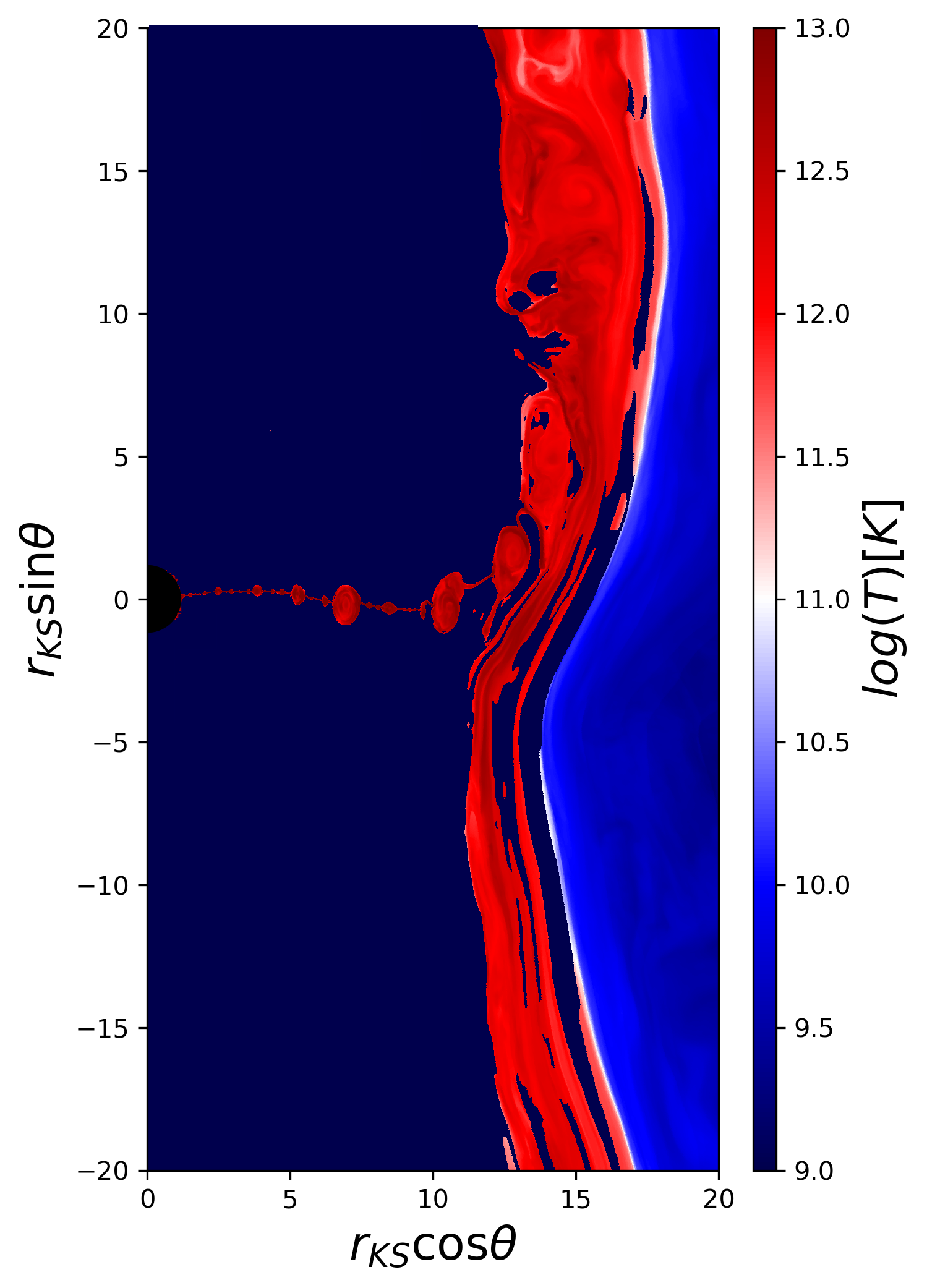
Figure 15: Limb-brightening of the jet sheath by hot plasmoids from the exhaust pf the equatorial current sheet. The color map shows the gas temperature, $T$[K], distribution at $t=3380r_{g}/c$ in the MAD retrograde case with $a=-0.9375$.

5 Discussion and conclusions

We have shown that plasmoids form ubiquitously due to magnetic reconnection in black-hole accretion flows, regardless of the initial size of the disk and the magnetization during the quasi-steady-state phase of accretion. Energetic plasmoids that form on the smallest resistive scales and escape the gravitational pull of the black hole can grow into macroscopic hot spots through coalescence with other plasmoids. In both MAD and SANE cases these hot structures are ejected either along the jet’s sheath or into the disk, heating the sheath and regions of the disk within a few Schwarzschild radii of the event horizon. In the MAD case the magnetization is significantly higher close to the event horizon, powering hot spots with relativistic temperatures $T=p/\rho\sim 10$, an order of magnitude higher than in the SANE case $T\sim 1$. The preferential heating of the jet’s sheath by continuous reconnection events close to the event horizon can potentially explain Very Long Baseline Interferometry (VLBI) observations of the black hole at the center of the galaxy M87 which clearly show a limb-brightened jet down to $7r_{g}$ (Ly et al. 2007; Kim et al. 2018).

In the SANE case current sheets and plasmoids also form in the turbulence induced by the MRI inside the disk. These plasmoids however do not reach relativistic temperatures due to the low magnetization in the disk.

In both MAD and SANE cases circular hot spots can reach radii of approximately $1-3r_{g}$ via plasmoid coalescence. The formation process from in-falling flux tubes to macroscopic hot spots of size $\sim\mathcal{O}(r_{g})$ occurs on a time scale of $\sim\mathcal{O}(100r_{g}/c)$, indicating a reconnection rate of $\sim 0.01c$. By analyzing multiple individual current sheets, we confirm reconnection rates between $0.01c$ and $0.03c$ for Lundquist numbers of $S\gtrsim 10^{5}$, in accordance with numerical relativistic resistive MHD studies of isolated plasmoid-dominated reconnection (e.g., Del Zanna et al. 2016; Ripperda et al. 2019b) and analytic predictions (Bhattacharjee et al. 2009; Uzdensky et al. 2010).

In all our simulations, regardless of spin and accretion state, plasmoids with a size of $\sim 1r_{g}$ form within $5-10r_{g}$ from the event horizon on time scales of $100r_{g}/c\approx 30$ minutes assuming conditions of Sgr A^∗, which is in accordance with orbiting hot spots observed by Gravity Collaboration et al. (2018, 2020). Although in reality hot spots orbit around the black hole, in our simulations we assume axisymmetry such that analyzing trajectories in the invariant azimuthal ($\phi$-)direction cannot be directly related to observations. Only MAD accretion disks around spinning black holes are consistent with observations of near-infrared and X-ray flares, where large magnetic field amplitudes of $10-50$G are observed in quiescence, and the field strength drops to $1-5$G at the peak of a flare (Dodds-Eden et al. 2009, 2010; Ponti et al. 2017), due to conversion of the magnetic energy into accelerated electrons and synchrotron emission through reconnection. We find that during a flare period in our MAD simulations energies $\gtrsim 10^{38}$ erg can be emitted from a spherical region of $1-3r_{g}$ within $30-45$ minutes. The flares are associated with events of reduced magnetic flux through the horizon and periodic reformation of the accretion flow (see the top panel of Fig. 6). Hints of the same process of cycles of flux build-up and dissipation have been observed in 3D MAD simulations by Dexter et al. (2020) and Porth et al. (2020). In our high-resolution SANE simulations there is no substantial variability in the current sheet and plasmoid formation which could be robustly associated with a flaring event.

Assuming axisymmetry prevents us from resolving non-axisymmetric instabilities that can potentially disrupt the current sheets forming close to the event horizon. In future work we plan to address whether plasmoid-structures can form in full 3D simulations and if they can result in orbiting hot spots. In 3D simulations we plan to trace test particles to model radiative signatures with realistic electron distribution functions (Ripperda et al. 2018, 2019a; Bacchini et al. 2018, 2019). The radiative properties of Sgr A^∗ have been studied in ideal GRMHD simulations by Davelaar et al. (2018), concluding that 5-10% of the electrons inside the jet’s sheath are expected to be accelerated to non-thermal distributions during a flare.

In this work we rely on numerical viscosity, such that the typical magnetic Prandtl number, indicating the ratio between viscosity and resistivity, is smaller than unity. In a future study we will analyze the effect of adding explicit viscosity and resistivity on plasmoid formation in MRI turbulence in shearing box simulations considering a range of Prandtl numbers.

References

- Alfvén (1942) Alfvén, H. 1942, Nature, 150, 405 EP
- Arnowitt et al. (1959) Arnowitt, R., Deser, S., & Misner, C. W. 1959, Phys. Rev., 116, 1322
- Bacchini et al. (2018) Bacchini, F., Ripperda, B., Chen, A. Y., & Sironi, L. 2018, ApJS, 237, 6
- Bacchini et al. (2019) Bacchini, F., Ripperda, B., Porth, O., & Sironi, L. 2019, ApJS, 240, 40
- Baganoff et al. (2001) Baganoff, F., Bautz, M., Brandt, W., et al. 2001, Nature, 413, 45-48
- Baganoff et al. (2003) Baganoff, F. K., Maeda, Y., Morris, M., et al. 2003, ApJ, 591, 891–915
- Balbus & Hawley (1991) Balbus, S. A., & Hawley, J. F. 1991, ApJ, 376, 214
- Ball et al. (2016) Ball, D., Özel, F., Psaltis, D., & Chan, C. 2016, ApJ, 826, 77
- Ball et al. (2018) Ball, D., Özel, F., Psaltis, D., Chan, C., & Sironi, L. 2018, ApJ, 853, 2
- Bessho & Bhattacharjee (2005) Bessho, N., & Bhattacharjee, A. 2005, Phys. Rev. Lett., 95, 245001
- Bhattacharjee et al. (2009) Bhattacharjee, A., Huang, Y.-M., Yang, H., & Rogers, B. 2009, Physics of Plasmas, 16, 112102
- Blandford & Znajek (1977) Blandford, R., & Znajek, R. 1977, MNRAS, 179, 3
- Boldyrev & Loureiro (2017) Boldyrev, S., & Loureiro, N. F. 2017, ApJ, 844, 125
- Bower et al. (2006) Bower, G. C., Goss, W. M., Falcke, H., Backer, D. C., & Lithwick, Y. 2006, ApJ, 648, L127–L130
- Bower et al. (2003) Bower, G. C., Wright, M. C. H., Falcke, H., & Backer, D. C. 2003, ApJ, 588, 331
- Boyce et al. (2019) Boyce, H., Haggard, D., Witzel, G., et al. 2019, ApJ, 871, 161
- Broderick & Loeb (2005) Broderick, A. E., & Loeb, A. 2005, MNRAS, 363, 353
- Chandrasekhar (1960) Chandrasekhar, S. 1960, Proceedings of the National Academy of Science, 46, 253
- Comisso et al. (2018) Comisso, L., Huang, Y.-M., Lingam, M., Hirvijoki, E., & Bhattacharjee, A. 2018, ApJ, 854, 103
- Davelaar et al. (2018) Davelaar, J., Mościbrodzka, M., Bronzwaer, T., & Falcke, H. 2018, A&A, 612, A34
- Davis et al. (2010) Davis, S. W., Stone, J. M., & Pessah, M. E. 2010, ApJ, 713, 52
- Del Zanna et al. (2016) Del Zanna, L., Papini, E., Landi, S., Bugli, M., & Bucciantini, N. 2016, MNRAS, 460, 4
- Dexter et al. (2020) Dexter, J., Tchekhovskoy, A., Jiménez-Rosales, A., et al. 2020. https://arxiv.org/abs/2006.03657
- Dodds-Eden et al. (2010) Dodds-Eden, K., Sharma, P., Quataert, E., et al. 2010, ApJ, 725, 450
- Dodds-Eden et al. (2009) Dodds-Eden, K., Porquet, D., Trap, G., et al. 2009, ApJ, 698, 676
- Dong et al. (2018) Dong, C., Wang, L., Huang, Y.-M., Comisso, L., & Bhattacharjee, A. 2018, Phys. Rev. Lett., 121
- Eckart et al. (2006) Eckart, A., Baganoff, F., Schödel, R., et al. 2006, A&A, 425, 934-937
- Event Horizon Telescope Collaboration et al. (2019a) Event Horizon Telescope Collaboration, Akiyama, K., Alberdi, A., et al. 2019a, ApJ, 875, L1
- Event Horizon Telescope Collaboration et al. (2019b) —. 2019b, ApJ, 875, L5
- Fazio et al. (2018) Fazio, G. G., Hora, J. L., Witzel, G., et al. 2018, ApJ, 864, 58
- Fishbone & Moncrief (1976) Fishbone, L., & Moncrief, V. 1976, ApJ, 207, 962-976
- Genzel et al. (2003) Genzel, R., Schödel, R., Ott, T., et al. 2003, Nature, 425, 934-937
- Goodman & Uzdensky (2008) Goodman, J., & Uzdensky, D. 2008, ApJ, 688, 1
- Gravity Collaboration et al. (2018) Gravity Collaboration, Abuter, R., Amorim, A., et al. 2018, A&A, 618, L10
- Gravity Collaboration et al. (2020) Gravity Collaboration, Bauböck, M., Dexter, J., et al. 2020, A&A, 635, A143
- Guo et al. (2014) Guo, F., Li, H., Daughton, W., & Liu, Y.-H. 2014, Phys. Rev. Lett., 113
- Gutiérrez et al. (2020) Gutiérrez, E. M., Nemmen, R., & Cafardo, F. 2020, ApJ, 891, L36
- Igumenshchev (2008) Igumenshchev, I. V. 2008, ApJ, 677, 317
- Igumenshchev et al. (2003) Igumenshchev, I. V., Narayan, R., & Abramowicz, M. A. 2003, ApJ, 592, 1042
- Kadowaki et al. (2019) Kadowaki, L. H. S., de Gouveia Dal Pino, E. M., & Medina-Torrejón, T. E. 2019. https://arxiv.org/abs/1904.04777
- Kim et al. (2018) Kim, J.-Y., Krichbaum, T. P., Lu, R.-S., et al. 2018, A&A, 616, A188
- Kruskal & Schwarzschild (1954) Kruskal, M. D., & Schwarzschild, M. 1954, Proc. R. Soc. Lond. A, 223
- Li et al. (2017) Li, Y.-P., Yuan, F., & Wang, Q. D. 2017, MNRAS, 468, 2552–2568
- Löhner (1987) Löhner, R. 1987, Computer Methods in Applied Mechanics and Engineering, 61, 323
- Loureiro et al. (2007) Loureiro, N., Schekochihin, A., & Cowley, S. 2007, Phys. of Plasmas, 14, 100703
- Loureiro & Uzdensky (2016) Loureiro, N. F., & Uzdensky, D. A. 2016, Plasma Physics and Controlled Fusion, 58, 014021
- Ly et al. (2007) Ly, C., Walker, R. C., & Junor, W. 2007, ApJ, 660, 200
- Mahlmann et al. (2020) Mahlmann, J. F., Levinson, A., & Aloy, M. A. 2020. https://arxiv.org/abs/2001.03171
- Markoff et al. (2001) Markoff, S., Falcke, H., Yuan, F., & Biermann, P. L. 2001, A&A, 379, L13
- Marrone et al. (2007) Marrone, D. P., Moran, J. M., Zhao, J.-H., & Rao, R. 2007, ApJ, 654, L57
- Marrone et al. (2008) Marrone, D. P., Baganoff, F. K., Morris, M. R., et al. 2008, ApJ, 682, 373
- Meyer et al. (2008) Meyer, L., Do, T., Ghez, A., et al. 2008, ApJ, 688, L17
- Narayan et al. (2003) Narayan, R., Igumenshchev, I. V., & Abramowicz, M. A. 2003, Publications of the Astronomical Society of Japan, 55, L69
- Narayan et al. (2012) Narayan, R., Sadowski, A., Penna, R. F., & Kulkarni, A. K. 2012, MNRAS, 426, 3241
- Nathanail et al. (2020) Nathanail, A., Fromm, C. M., Porth, O., et al. 2020. https://arxiv.org/abs/2002.01777
- Neilsen et al. (2013) Neilsen, J., Nowak, M., Gammie, C., et al. 2013, ApJ, 774, 1
- Olivares et al. (2019) Olivares, H., Porth, O., Davelaar, J., et al. 2019, A&A, 629, A61
- Orszag & Tang (1979) Orszag, S. A., & Tang, C.-M. 1979, Journal of Fluid Mechanics, 90, 129
- Parfrey et al. (2014) Parfrey, K., Giannios, D., & Beloborodov, A. M. 2014, MNRAS: Letters, 446, L61–L65
- Parfrey et al. (2019) Parfrey, K., Philippov, A., & Cerutti, B. 2019, Phys. Rev. Lett., 122, 035101
- Ponti et al. (2017) Ponti, G., George, E., Scaringi, S., et al. 2017, MNRAS, 468, 2447
- Porth et al. (2020) Porth, O., Mizuno, Y., Younsi, Z., & Fromm, C. M. 2020. https://arxiv.org/abs/2006.03658
- Porth et al. (2017) Porth, O., Olivares, H., Mizuno, Y., et al. 2017, Computational Astrophysics and Cosmology, 4, 1
- Porth et al. (2019) Porth, O., Chatterjee, K., Narayan, R., et al. 2019, ApJS, 243, 26
- Ressler et al. (2020) Ressler, S. M., White, C. J., Quataert, E., & Stone, J. M. 2020, ApJ, 896, L6
- Ripperda et al. (2018) Ripperda, B., Bacchini, F., Teunissen, J., et al. 2018, ApJS, 235, 1
- Ripperda et al. (2019a) Ripperda, B., Porth, O., & Keppens, R. 2019a, in Journal of Physics Conference Series, Vol. 1225, 012018
- Ripperda et al. (2019b) Ripperda, B., Porth, O., Sironi, L., & Keppens, R. 2019b, MNRAS, 485, 299
- Ripperda et al. (2019c) Ripperda, B., Bacchini, F., Porth, O., et al. 2019c, ApJS, 244, 10
- Rowan et al. (2017) Rowan, M., Sironi, L., & Narayan, R. 2017, ApJ, 850, 1
- Sadowski et al. (2013) Sadowski, A., Narayan, R., Tchekhovskoy, A., & Zhu, Y. 2013, MNRAS, 429, 4
- Sironi & Spitkovsky (2014) Sironi, L., & Spitkovsky, A. 2014, ApJL, 783, 1
- Tomei et al. (2020) Tomei, N., Del Zanna, L., Bugli, M., & Bucciantini, N. 2020, MNRAS, 491, 2346
- Uzdensky et al. (2010) Uzdensky, D., Loureiro, N., & Schekochihin, A. 2010, Phys. Rev. Lett., 105, 23
- van der Holst et al. (2008) van der Holst, B., Keppens, R., & Meliani, Z. 2008, Computer Physics Communications, 179, 617–627
- Velikhov (1959) Velikhov, E. P. 1959, J. Exptl. Theoret. Phys., 36, 1398
- Vourellis et al. (2019) Vourellis, C., Fendt, C., Qian, Q., & Noble, S. C. 2019, ApJ, 882, 2
- Werner et al. (2018) Werner, G., Uzdensky, D., Begelman, M., Cerutti, B., & Nalewajko, K. 2018, MNRAS, 473, 4
- Werner et al. (2015) Werner, G. R., Uzdensky, D. A., Cerutti, B., Nalewajko, K., & Begelman, M. C. 2015, ApJ, 816, L8
- White et al. (2016) White, C. J., Stone, J. M., & Gammie, C. F. 2016, ApJS, 225, 22
- White et al. (2019) White, C. J., Stone, J. M., & Quataert, E. 2019, ApJ, 874, 168
- Younsi & Wu (2015) Younsi, Z., & Wu, K. 2015, MNRAS, 454, 3283
- Yuan et al. (2004) Yuan, F., Quataert, E., & Narayan, R. 2004, ApJ, 606, 894–899
- Yuan et al. (2019a) Yuan, Y., Blandford, R. D., & Wilkins, D. R. 2019a, MNRAS, 484, 4920–4932
- Yuan et al. (2019b) Yuan, Y., Spitkovsky, A., Blandford, R. D., & Wilkins, D. R. 2019b, MNRAS, 487, 4114–4127
- Zhdankin et al. (2013) Zhdankin, V., Uzdensky, D. A., Perez, J. C., & Boldyrev, S. 2013, ApJ, 771, 124
- Zhdankin et al. (2017) Zhdankin, V., Walker, J., Boldyrev, S., & Lesur, G. 2017, MNRAS, 467, 3620–3627
- Zhu & Stone (2018) Zhu, Z., & Stone, J. M. 2018, ApJ, 857, 34